Pricing and Collaboration in Last Mile Delivery Services

Abstract

Recently, last mile delivery has emerged as an essential process that greatly affects the opportunity of obtaining delivery service market share due to the rapid increase in the business-to-consumer (B2C) service market. Express delivery companies are investing to expand the capacity of hub terminals to handle increasing delivery volume. As for securing massive delivery quantity by investment, companies must examine the profitability between increasing delivery quantity and price. This study proposes two strategies for a company’s decision making regarding the adjustment of market density and price by developing a pricing and collaboration model based on the delivery time of the last mile process. A last mile delivery time function of market density is first derived from genetic algorithm (GA)-based simulation results of traveling salesman problem regarding the market density. The pricing model develops a procedure to determine the optimal price, maximizing the profit based on last mile delivery time function. In addition, a collaboration model, where a multi-objective integer programming problem is developed, is proposed to sustain long-term survival for small and medium-sized companies. In this paper, sensitivity analysis demonstrates the effect of delivery environment on the optimal price and profit. Also, a numerical example presents four different scenarios of the collaboration model to determine the applicability and efficiency of the model. These two proposed models present managerial insights for express delivery companies.

1. Introduction

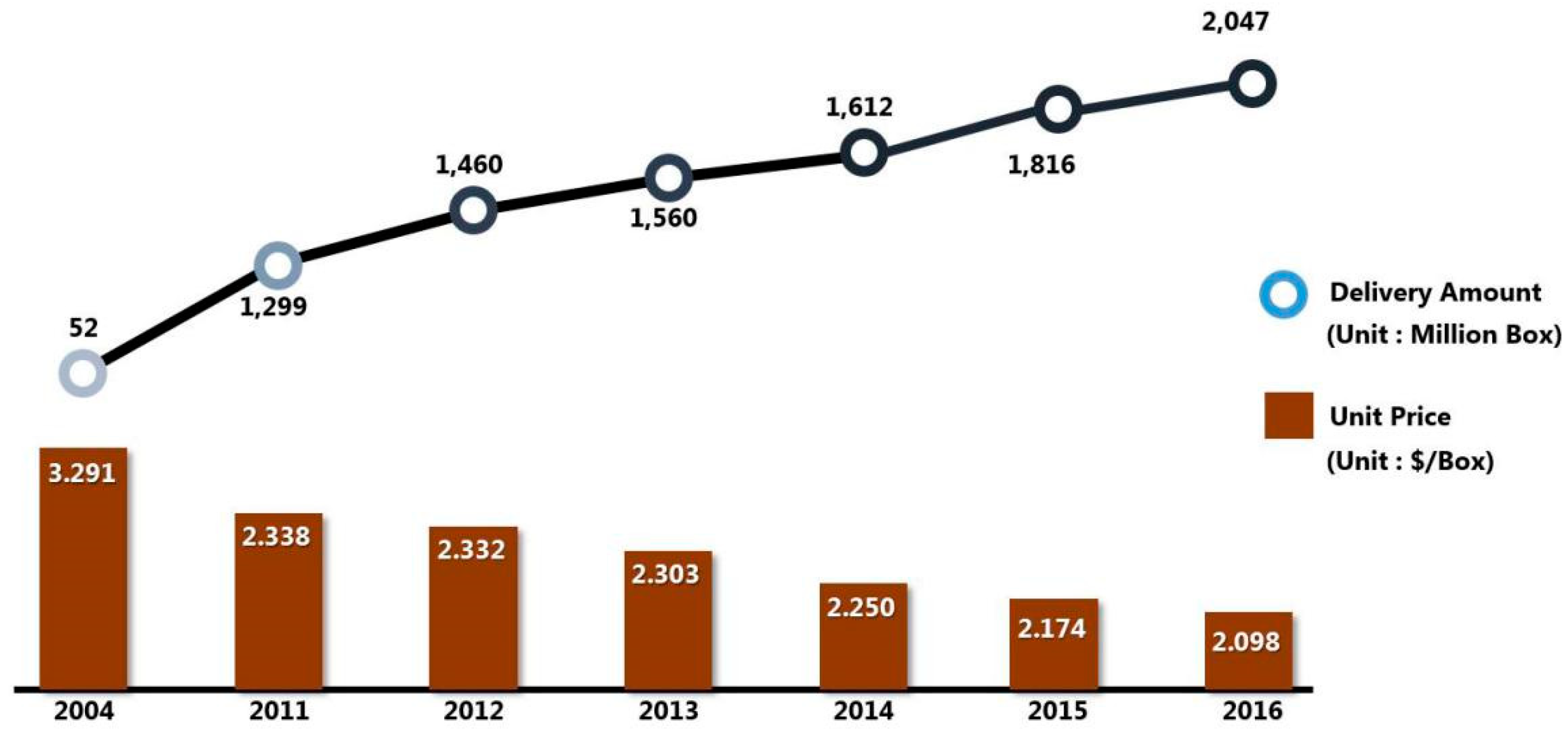
A rapid increase in indirect purchases is accelerating a steep surge of express delivery service market. This incremental result is mainly due to an increasing consumption through online-based transactions such as internet shopping, mobile shopping and TV home shopping, which has naturally led to a growth of express delivery services. Figure 1 shows the recent trend for the courier market in Korea. It is observed that the courier amount has continuously been growing year by year. On the other hand, the unit price has been dropping due to the greater competition among courier service providers [1]. At the end of the day, the express delivery companies with low market share are not likely to survive in competitive market and cannot help avoiding collaboration for increasing their market shares company. More than 80% of market is occupied by only five companies and especially, about 67% is by three companies and a big on covers 45% of entire market [1].

Based on a recent article by Business Insider their shares of delivery costs are reported to be 4%, 37%, 6% and 53%, respectively [2].

Many researches related to the express delivery companies focused on cost minimization by varying network distances. Therefore, since the transport networks managed by express delivery companies already reflect delivery environment, it can be said that express delivery companies are using the optimal route. In addition, hub location problem, which is dealt with express delivery related researches, is also reflected well in the real world. Thus, cost reduction through relocation of the hub terminal is not easy since express delivery companies’ hub terminals are already located in near optimal locations. Therefore, profit maximization through cost reduction from other processes is needed instead of cost minimization through changing already existing networks.

As delivery supply is increasing immensely every year, the express delivery companies are planning enormous investments in expansion of hub terminals to handle increased delivery amount. However, as expanded hub terminals deal with increased supply, securing massive delivery quantity raises another problem. In order to obtain increasing delivery quantity, price reduction can be one solution, but there needs to be a fundamental solution if the investment is on large scale to secure delivery supply that will guarantee the company’s profitability.

This study emphasizes delivery amounts as market density in perspective of delivery service company and proposes a pricing model to confirm profitability in consideration of the market density. Also the variation of maximum profit in regards of price changes through the analysis of the pricing model is suggested. In addition, this paper suggests the collaboration model as a solution to increase competitiveness and to secure delivery quantity to small and medium-sized companies, to whom massive investment is difficult. This model is a strategy for small and medium-sized companies to win competitiveness against major companies. Also through collaboration, participating companies can reduce cost and increase profit through collaboration and decrease the CO₂ emission quantity generated through transportation simultaneously. With respect to these two solutions, we suggest managerial insight on market density and pricing with sensitivity analysis and numerical example.

The rest of the paper consists of the following: Section 2 introduces the previous studies related to pricing and collaboration of express delivery companies. Section 3 describes the definition of pricing and collaboration of express delivery companies. Section 4 demonstrates two types of mathematical models. Section 5 shows two numerical examples. Section 6 suggests managerial insights gained by analyzing the results from Section 5. Lastly, Section 7 provides the conclusion and further research prospects.

2. Literature Review

2.1. Last Mile Delivery

While many analytical studies related to express delivery services have been undertaken, the literature dealing with the market density and price decision in the last mile delivery services is scarce. Boyer et al. evaluated the effects of customer density and delivery window patterns in the last mile delivery process [3]. They performed a simulation where customer density and delivery window length were considered as variables and analyzed the effect on the last mile route efficiency. Gevaers et al. developed a last mile typology and instrument to simulate the total last mile costs. The transportation cost was derived through considering the transportation time and distance [4]. Kim et al. analyzed the impact of increasing demand on the parcel distribution network structure in terms of minimizing transportation and sortation costs [5]. Alibeyg et al. developed the net profit model that maximizes profit due to the routing commodities, which mainly focused on network design to maximize the net profit [6]. Zhou et al. suggested a location-routing problem with simultaneous home delivery and customer pickup [7]. Hu et al. proposed a vehicle routing problem with hard time windows under demand and travel time uncertainty [8]. The object of the model is to minimize the number of vehicle routes and total travel distance. Xuefeng et al. suggested a multi-objective location-routing problem with simultaneous pick-up and delivery [9]. Zhou et al. proposed a bi-level multi-sized terminal location-routing problem with simultaneous home delivery and customer pickup [10]. Regarding market density or demand for delivery services, Felisberto et al. introduced recipient pricing in the postal sector and tested with Swiss post data by considering the area and the amount of congestion [11]. Cebecauer et al. used Open Street Map data to model the demand points which approximate the geographical location of customers, and the road network, which is used to access or distribute services. They considered all inhabitants as customers, using population grids, and compared two different demand models by estimating the optimal structure of a public service system due to the differences between population grids [12].

2.2. Pricing Decision

Numerous studies have been undertaken in various industry fields related to the price-demand model. Mills introduced a single-period newsboy model with a linear demand function [13]. Polatoglu considered simultaneous pricing and procurement decisions associated with a single-period pure inventory model under deterministic or probabilistic demand [14]. Abad investigated a dynamic pricing and lot-sizing problem with a more general demand function [15]. Hong and Lee proposed model that the price and guaranteed lead time decision of a supplier offering guaranteed lead time for product including a lateness penalty [16]. The expected demand is suggested in a function of the price, guaranteed lead time and lateness penalty. Hong and Lee also proposed an optimal time-based consolidation policy with price sensitive demand [17]. They considered a single-item inventory system where shipments are consolidated to reduce the transportation and developed a mathematical model to obtain the optimal price, replenishment quantity and dispatch cycle to maximize the total profit. Ahmadi-Javid et al. considered a profit-maximization location-routing problem with price-sensitive demands [18]. The problem determined the location of facilities, the allocation of vehicles and customers to established facilities and the pricing and routing decisions in order to maximize the total profit.

2.3. Collaboration

Related research on collaboration have been studied in various industry fields have been studied. Cruijssen et al. measured the dependence of the synergy on a number of characteristics of the distribution problem under consideration and found that significant cost savings are achieved [19]. Lozano et al. suggested a linear model to study the cost savings through forming the transportation [20]. They solved an optimization model for different collaboration scenarios. Kimms and Kozeletskyi suggested a cost allocation scheme for a horizontal cooperation among traveling salesmen providing expected costs for the coalition members [21]. They calculated cost allocation by using the core concept. Wang et al. suggested a collaborative multiple centers vehicle routing problem with simultaneous delivery and pickup to minimize operating cost and the total number of vehicles in the network [22]. They proposed a hybrid heuristic algorithm combining k-means and non-dominating sorting genetic algorithm (GA). Cheung et al. proposed an integer programming model for collaborative service network design by sharing service centers [23]. Ferdinand et al. suggested a collaboration model considering pick-up and routing problem of line-haul vehicles for maximizing the profits of participating companies [24].

In this paper, the travel time was computed through considering market density in unit delivery area and developed the function of last mile delivery time regarding market density (LMF) by solving the travelling salesman problem (TSP) by using GA. Most of the studies dealing with price and cost in last mile delivery and express delivery considered minimizing the cost through optimizing the network design. They also converted transportation time into cost with coefficient values. Instead, we suggest LMF converts market density into demand and computes travel time. The relationship between delivery service and market density was studied before by [3], however, they only performed a simulation experiment and did not suggest any models. We propose LMF and the pricing model which considered market density and travel time simultaneously. The profitability in last mile delivery is computed in the pricing model by considering the changes in the market density and travel time. The pricing model decides the optimal price to maximize the profit which was used in various industries for a long time. As our study focuses on the price decision in last mile delivery, we calculate the travel time by considering the market density and converting it into a linear demand function [15]. By applying the LMF into the pricing model, more realistic-pricing model for the last mile delivery process was proposed, and observed the effect of the market density in the travel cost, optimal price and profit from last mile delivery. In addition we propose the collaboration model for last mile delivery companies. Participating companies share terminals in separate delivery regions and consider which terminal to share. The incremental profit is calculated. The total profit from collaboration is computed by using max–min criteria.

3. Problem Statement

In the era of time-based competition, today’s customers begin to demand responsiveness as an integral part of a service. As consumers increasingly turn to e-commerce for all their shopping needs, a quick response service becomes a critical mission for logistic companies and retail partners across the world. Express delivery companies have made several types of efforts for speedy fulfilment, most of which are focused on a delivery service network, terminal productivity and vehicle routing and scheduling, etc. Recently, last mile delivery as the final step of the delivery process, has emerged as a hot issue in fast delivery. As described earlier by Business Insider, the share of last mile is 53%, the highest of the elements of delivery cost [2]. In addition, last mile can be a key to customer satisfaction since it becomes the contact point at which the parcel finally arrives at the buyer’s door.

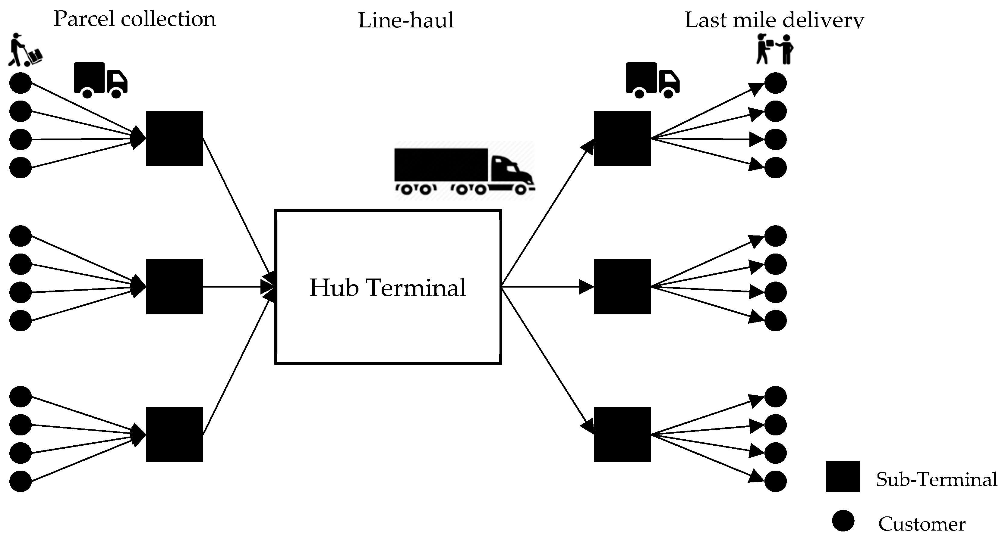
The objective of this study is to emphasize the impact of market density on price decision and forming the strategic alliance. First, we propose the delivery time-market density model. Secondly based on the time-market density model, two kinds of strategies to survive in the express delivery market are suggested; adjusting the price to maximize the profit, and reducing the transportation cost by forming a collaboration. In general, an express delivery service network consists of customer, service centers and consolidation terminals. Customers can be classified into three sub-regions: residential; industrial; commercial areas, where customers either ship or receive ordered parcel items. The service centers are used as a transshipment and temporary storage facility connecting customers to a consolidation terminal. At the consolidation terminal, customer orders are consolidated into larger shipments, mixed and then loaded onto delivery trucks for local deliveries [25]. This study mainly focuses on the last mile of the final step of the shipment process, which is depicted in Figure 2.

This study is divided into three sub-problems: First, an approximate function of last mile delivery time regarding market density (LMF) is derived using GA-based simulation results of traveling salesman problem with randomly generated customers. Next, according to LMF, a procedure is carried out for searching an optimal price for maximizing profit. Lastly, a collaborative delivery system is suggested for extending market share. For these purpose we make the following underlying assumptions throughout the paper:

(1)

Annual delivery service demand is evenly distributed and depends on the delivery service price.

(2)

Market share of each express delivery service company is the same in all service areas regardless of regional characteristics, which affects last mile delivery time.

(3)

Moving truck/worker and transaction to recipient, transaction time is ignored.

(4)

Although delivery costs comprise collection, sorting, line-haul and last mile costs, other costs excluding last mile cost are constant regardless of service price.

(5)

Most last mile delivery services are operated in one shift per day. However, delivery services in some companies are performed in two or three shifts in a day.

(6)

Daily working time for each express delivery company is the same.

4. Model Design

This section describes two methodologies to increase competitiveness of delivery companies; the first one is to increase their profit by controlling delivery service price and the second one is to introduce a collaborative delivery system for occupying stable market share. Prior to developing the system methodologies, a change of last mile delivery time related to market share is investigated.

4.1. Last Mile Delivery Time Function with Respect to Market Density

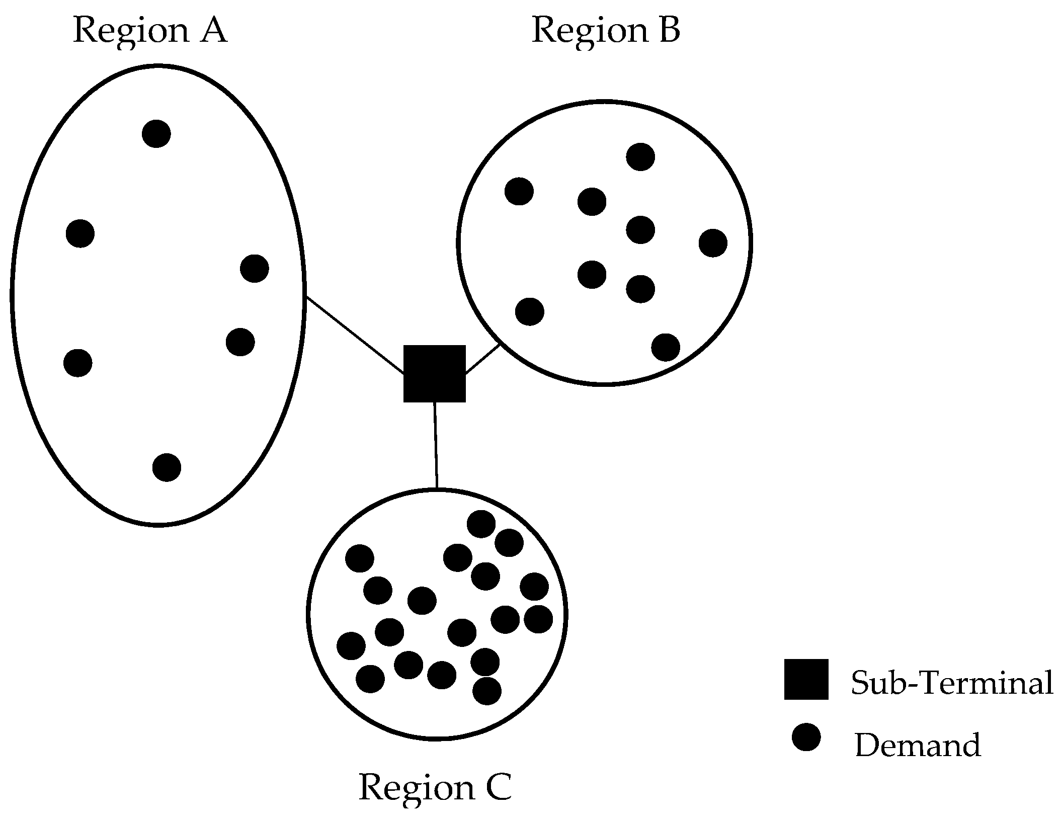
In order to observe a trend of last mile delivery time related to market share, actual delivery data was collected from three regions of a Korean express delivery company, which are shown in Figure 3. The company operates three shifts in a day and has around 40% market share in express delivery service market in Korea. It can be observed that the last mile delivery time depends on the attributes of service areas. If we can derive a relation equation of last mile delivery time versus market density, last mile delivery time for each service region can be found under the assumption that market share and attributes of regions are given.

For this purpose, a simulation for gathering last mile delivery data according to density has been carried out. The data is obtained by solving the TSP. The procedure for deriving a last mile delivery function of market density is described as follows:

(Step 1)

Generate random demand points within unit square. At this time, we assume that the market density is 10% if 10 demand points are generated.

(Step 2)

Solve TSP by a GA-based heuristic assuming that the position of service center is located at (0, 0) and then calculate the average moving time. For every market density, 100 experiments are done.

(Step 3)

By continuously increasing demand points by 10 up to 100(%) demand points, the average traveling time is calculated. It is performed under the assumption that all generated demand can be served by only a truck.

(Step 4)

If we denote market density as an independent variable, we can find an approximate LMF.

(Step 5)

Define a time shape as an average last mile delivery time to a LMF value with the same market share. Then we can estimate a trend of last mile delivery time according to the change of market share.

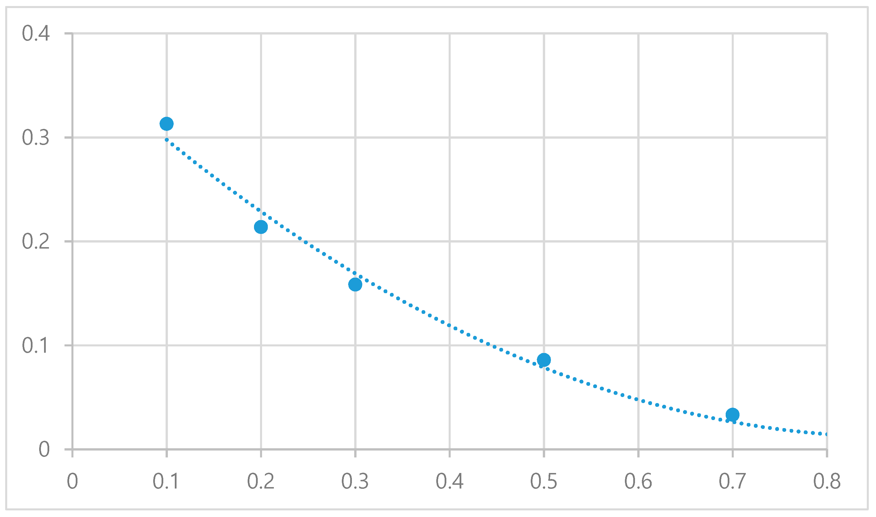
With average delivery time related to market density from the results of the GA heuristic in

Table 1. Average last mile delivery time from the genetic algorithm (GA) results.

Market Density	0.1	0.2	0.3	0.5	0.7
Delivery time per box	0.3129	0.2137	0.1583	0.0859	0.0331

, the LMF, depicted in Figure 4, can be expressed as:

$$\mathrm{f}\left(\pi \right) = 0.00005{\pi }^2-0.8347\pi +0.3764$$

(1)

where $\pi$ denotes market density and a coefficient of determination, $R^2$ is 0.9896.

If data collection and analysis for some service regions is performed, we can calculate the time shapes for the service regions, which enables us to estimate the trend in unit last mile delivery time according to market share.

4.2. Pricing Model

In this section, the pricing model for an express delivery service considering the average last mile delivery time according to market share of the company is developed. The objective of the model is to maximize the profit of express delivery company by adjusting the unit delivery price. Reducing the price can expand market share and increase possible customer density, which can provide unit delivery cost, especially last mile delivery cost. Prior to developing the profit model, the following notations are introduced.

Notations for Pricing Model

$p$	Unit delivery price
$c$	Unit last mile delivery cost
$D\left(p\right)$	Delivery demand function, which is defined as $a-bp$, where $a>0$ and $b>0$
$N$	Total delivery demand in certain region
$t$	Average last mile delivery time per delivery service
$T$	Daily working time
d	Daily delivery amount
w	Daily cost for last mile delivery worker, i.e., daily worker income
$K$	Other delivery cost excluding last mile delivery cost

Model Design

In order to establish the profit model, unit last mile delivery cost is firstly derived with the relationship between daily delivery amount and last mile delivery time per delivery service. The daily delivery amount during working time can be represented as:

$$d = \frac{T}{t}$$

(2)

with daily delivery amount, daily delivery worker cost becomes:

$$w = c\times d$$

(3)

Assuming that w is constant regardless of service areas, unit last mile delivery cost, $c$ is obtained by:

$$c = \frac{w}{d} = w\times \frac{t}{T}$$

(4)

This means that last mile delivery cost for each service region depends on average last mile delivery time, which is expressed as a function of market density. From now on, market share is derived with unit delivery price. If total delivery demand, $N$ and the demand for a company in any region, $D\left(p\right)$ are given, the density for the company is defined as $\frac{D\left(p\right)}{N}$. According to Abad et al.’s linear demand function [15], the demand function in this paper is referred as a linear demand rate function of price, $D\left(p\right) = a-bp$, where a$>0$ and $b>0$. With $D\left(p\right)$ and (1), unit last mile delivery cost, $c$ can be represented as a function of unit delivery price, $c\left(p\right)$, which is:

$$c\left(p\right) = w\times \frac{\left(0.00005\right){\left(\frac{a-bp}{N}\right)}^2-0.8347\left(\frac{a-bp}{N}\right)+0.3764}{T}$$

(5)

Therefore, the pricing model is defined as:

$$\mathrm{Max} Z\left(p\right) = \left(p-c\left(p\right)\right)D\left(p\right)-K$$

(6)

$$\mathrm{where} 0< p <\frac{a}{b}$$

(7)

In the objective Function (6) K means other delivery service cost excluding last mile delivery cost such as collection, terminal operating and line-haul costs, etc. and is assumed to be independent of p. Since $Z\left(p\right)$ is a polynomial function of p, we can find an optimal solution considering the constraint (7). The optimal price for profit maximization is found in the pricing model. In order to obtain an optimal solution, we evaluate the optimal price to maximize the profit through differentiation. Since the objective function is a cubic function, we obtain two different optimal prices. Also, since the delivery demand follows a function of $D\left(p\right) = a-bp$, the delivery demand needs to be larger than 0. Thus, the optimal price should be within the range of $0<p<\frac{a}{b}$. We seek the existing optimal price within the corresponding range and derive maximum profit relative to the optimal price. The calculation of the optimal price and profit is explained precisely in the Appendix A.

4.3. Collaboration Model

In this section, the collaboration model for express delivery service to expand market share of the company is proposed. While the pricing model is recommended for most companies regardless of their market shares, the collaboration model is mainly applied to small and medium-sized delivery companies.

A mathematical model for collaborative last mile delivery is developed to maximize the incremental profit of each participating express delivery company by saving last mile delivery cost. Suppose there is a county with n service regions, which are served with m express delivery companies. Each company has a relatively small delivery amount, which incurs a higher last mile delivery cost compared to the companies with lager market share. Collaborative delivery is proposed to expand their service density, and ultimately to decrease last mile deliver cost. The collaboration implements as follows:

(a)

In most service regions, only a single company can do a last mile delivery service.

(b)

The delivery amounts of the other companies are all assigned to the selected company after collaboration.

The following notations are introduced to establish a multi-objective integer programming model for collaborative last mile delivery:

Notations for Collaboration Model

$I$	Set of express delivery companies, I = {1,2,…,m}
$J$	Set of service regions in which service centers are to be merged, J = {1,2,…,n}
$c_{ij}$	Unit delivery cost of company i in the service region j, i$\in$I, j$\in$J
$t_{ij}$	Unit delivery time of company i in service region j, i→$\in$I, j$\in$J
$d_{ij}$	Daily delivery amount of company i within the merging region j, i$\in$I, j$\in$J
$D_j$	Total delivery amount of collaborating companies in service region j, j$\in$J
$c_j^1$	Unit delivery cost after alliance in the service region j, i$\in$I, j$\in$J
$c_j^2$	Unit mandated delivery cost after alliance in the service region j, i$\in$I, j$\in$J
$t{s}_j$	Time shape of service region j representing regional attribute, j$\in$J
$x_{ij}$	Binary variable such that xij = 1, if company i is responsible for service region j after alliance, xij = 0 otherwise, i$\in$I, j$\in$J
$L_i$	Lower bound for number of service regions of company
$U_i$	Upper bound for number of service regions

Model Formulation

Since last mile delivery time of company $i$ for a service region $j$ is obtained by multiplying time shape $t{s}_j$ and the value from (1), therefore, we can derive last mile delivery cost, $c_{ij}$ for each company from (1) and (4).

After applying a collaborative last mile delivery service, the incremental profit of company $i$ through an alliance can be divided into three portions. First, if company $i$ is responsible for service region $j$, the incremental profit for its own demand becomes $(c_{ij}-c_j^1)d_{ij}{x}_{ij}$. In addition, the company can get the profit, $(c_j^2-c_j^1)\times \left(D_j{x}_{ij}-d_{ij}\right)$ for the demands of the other companies. On the other hand, even if company $i$ does not have a right to do a delivery service in the service region $j,$ its incremental profit for its own demand is $(c_{ij}-c_j^2)\times d_{ij}\left(1-x_{ij}\right)$. Then by summing the three portions of incremental profits of company $i$, the objective function for company $i$ can be derived as follows (8):

$$\mathrm{Max} g_i\left(x\right) = {\displaystyle \sum }_j[(c_j^2-c_j^1)\left(D_j+d_{ij}\right)x_{ij}+\{c_{ij}+c_j^1-2c_j^2\}{d}_{ij}]$$

(8)

Therefore, the collaboration model can be formulated as multi-objective integer programming model with $m$ objective functions:

$$\begin{array}{c}\mathrm{Max} g_1\left(x\right) = {\displaystyle \sum _j}[(c_j^2-c_j^1)\left(D_j+d_{1j}\right)x_{1j}+\{c_{1j}+c_j^1-2c_j^2\}{d}_{1j}]\\ ⋮\\ \mathrm{Max} g_m\left(x\right) = {\displaystyle \sum _j}[(c_j^2-c_j^1)\left(D_j+d_{mj}\right)x_{mj}+\left\{c_{mj}+c_j^1-2c_j^2\right\}{d}_{mj}]\end{array}$$

(9)

Subject to,

$${\displaystyle \sum }_{i\in I}{x}_{ij} = 1, j\in J$$

(10)

$$L_i\le {\displaystyle \sum }_{j\in J}{x}_{ij}\le U_i, i\in I$$

(11)

$$x_{ij}\in \left\{0,1\right\}, i\in I, j\in J$$

(12)

The objective Function (9) represents the sum of incremental profit obtained through collaboration. Constraint (10) assures that only one service center can be selected for the last mile delivery service in each service region. Constraint (11) implies that the number of service regions should belong to the controlled range. Finally, Constraint (12) represents a binary variable as decision variables showing which company is responsible for each service region. Since in the mathematical model there are m objective functions representing the net profit increases of m companies, there exists a trade-off relationship with each other.

The proposed collaboration model is a multi-objective assignment problem where the objective is to maximize the incremental profit by forming a collaboration. Under the assumption that only one terminal is used in one region, we calculated reduced cost and incremental profit for participating companies by using max–min criteria. Also, we evaluated the determination of which company’s terminal in the region will be used.

The maximum profit of the objective function is derived in usage of max–min criteria. This collaboration methodology is used to reduce the rate of imbalance rate of distribution of the total profit from collaboration to compromise the optimal solution in the win–win situation of each company.

5. Numerical Example

Two illustrative examples are provided to explain the appropriateness of the pricing and collaboration model. We performed sensitivity analysis for the pricing model considering parameter values in the model. Also, we calculated incremental profit by using collaboration model in 4 different scenarios

5.1. Pricing Model

The following parameters are used in the first case. $a = 200$, $b = 30,K = 1 \mathrm{and}$ N = 800. We assume that daily total working hours are $T\in \left[9,10,11\right]$. We examined how difference in labor cost and working time affects optimal price and profit.

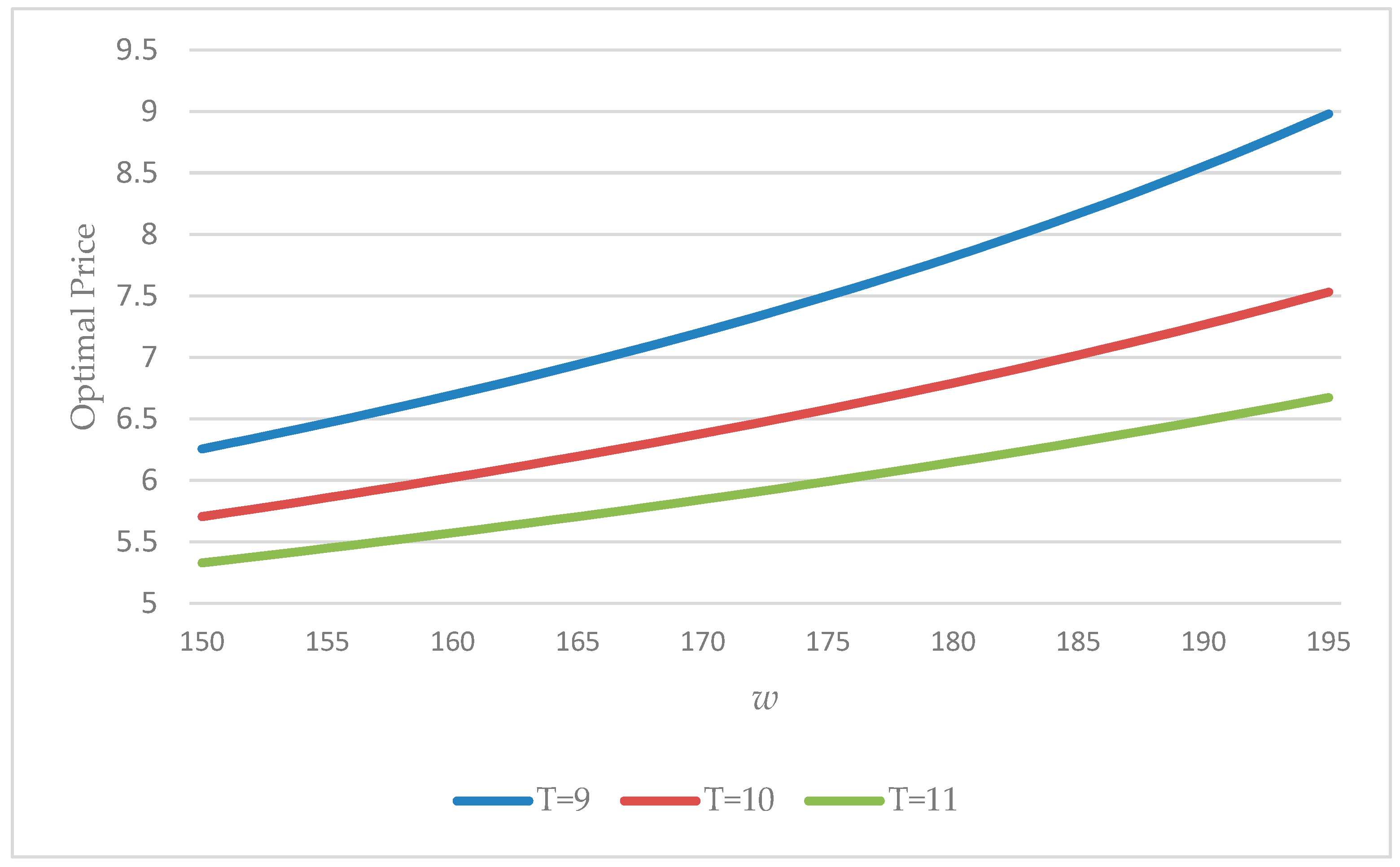
From

Table 2. The optimal price and the profit with w for different values of T (N = 800).

w	Optimal Price			Profit
	T = 9	T = 10	T = 11	T = 9	T = 10	T = 11
150	6.2555	5.70465	5.32854	1.425887	13.72849	29.78912
155	6.466826	5.858183	5.447527	−0.44777	9.095547	23.92256
160	6.694724	6.021343	5.572731	-	5.236412	18.55562
165	6.941222	6.195066	5.70465	-	2.226224	13.72849
170	7.208695	6.38041	5.843841	-	0.150178	9.485806
175	7.499937	6.578584	5.990921	-	−0.89474	5.877254
180	7.818266	6.790967	6.146581	-	-	2.958326
185	8.167645	7.019143	6.311595	-	-	0.791176
190	8.552851	7.264943	6.486831	-	-	−0.55434
195	8.979691	7.530491	6.67327	-	-	−0.99942

and Figure 5, the optimal price increases as the labor cost increases. As for an express company, when the labor cost increases, it has to increase the price in order to secure the least profit. When daily working time is short, the optimal price increase.

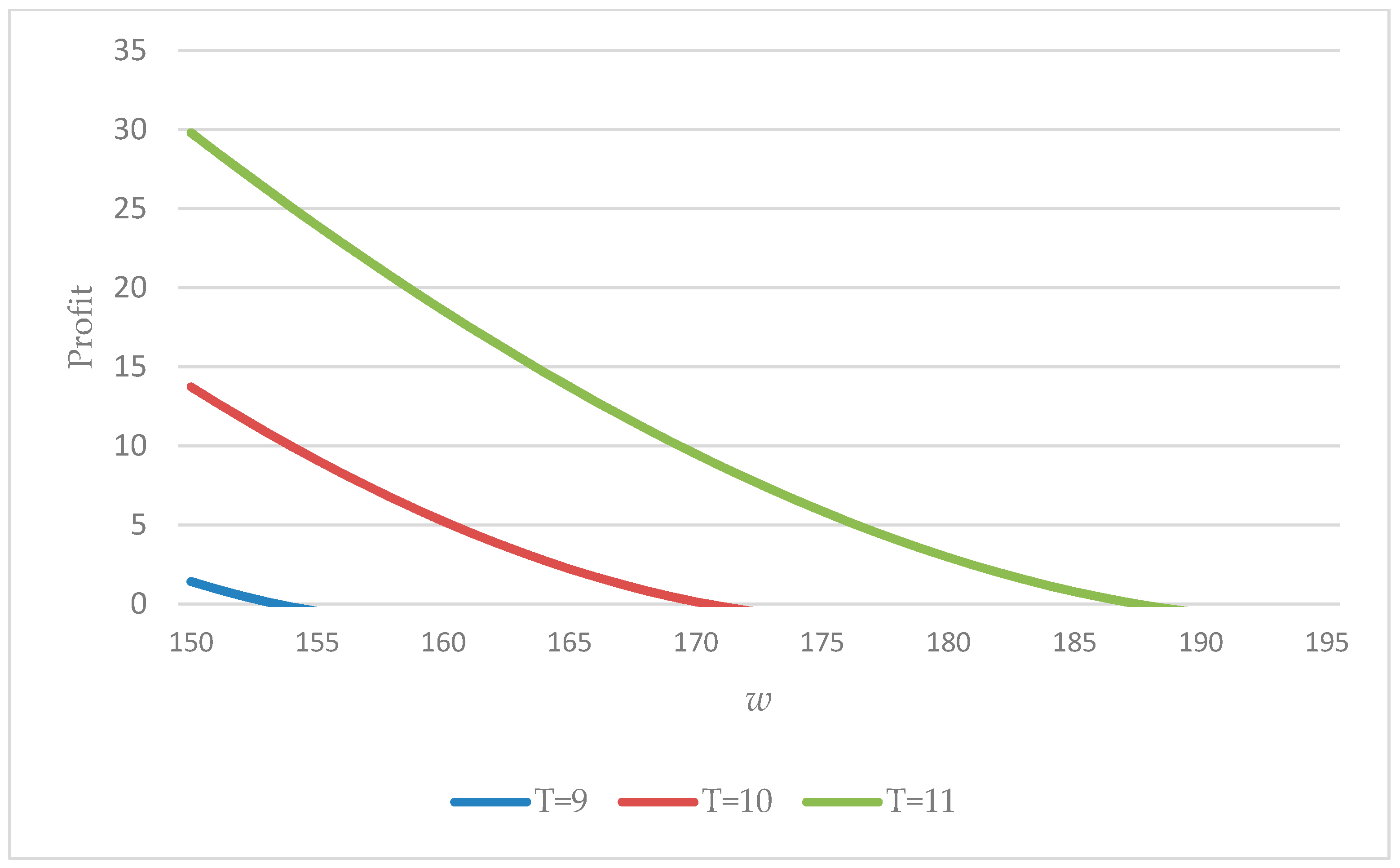
Figure 6 shows the variation of the profit when labor cost and daily working time differ. When labor cost increases, the profit decreases. A company can see the certain point where the profit may not occur from the delivery when labor cost reaches a certain point. Difference in daily working time affects the decreasing rate of profit as labor cost increases. This shows that a company cannot increase labor cost infinitely, and it can calculate the standard for the labor cost.

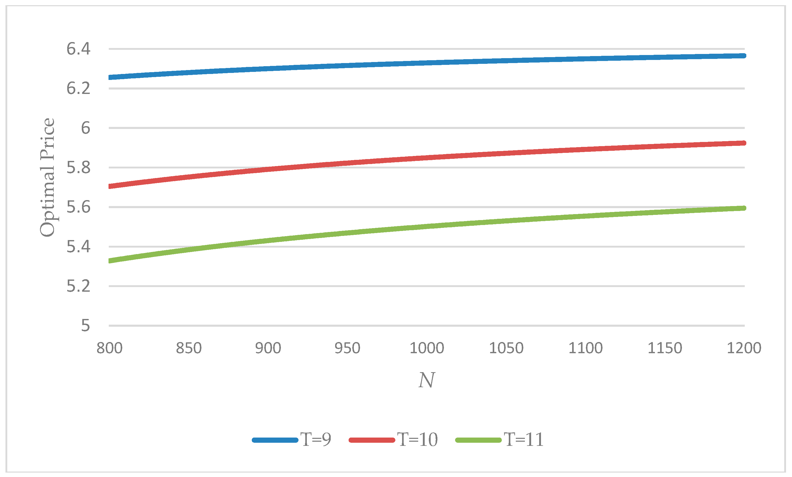
We then performed another case where a = 200, b = 30, K = 1 and w = 150. We assume that daily total working hours are T $\in$ [9,10,11].

Table 3. The optimal price and the profit with N for different values of T (w = 150).

N	Optimal Price			Profit
	T = 9	T = 10	T = 11	T = 9	T = 10	T = 11
800	6.2555	5.70465	5.32854	1.425887	13.72849	29.78912
850	6.280289	5.752257	5.384697	1.279631	12.99963	28.49699
900	6.299942	5.790785	5.430799	1.163678	12.40976	27.4362
950	6.315905	5.822606	5.469326	1.069494	11.92258	26.54974
1000	6.329129	5.84933	5.502002	0.991475	11.51343	25.79788
1050	6.340262	5.872092	5.530067	0.925788	11.16495	25.15214
1100	6.349765	5.891711	5.554432	0.869723	10.86457	24.59153
1150	6.35797	5.908797	5.575783	0.82131	10.60299	24.10025
1200	6.365127	5.92381	5.594647	0.779083	10.37313	23.6662

explains the difference in optimal price and profit when total delivery demand in certain delivery region changes.

Figure 7 shows the difference in rate of optimal price when total delivery demand changes. The increase in total delivery demand in a region is equal to the decrease in the market density. Therefore, the price increases when the market density decreases. The effect of the total working time to the optimal price showed similar results as the first case. When total working time increases, the optimal price increases.

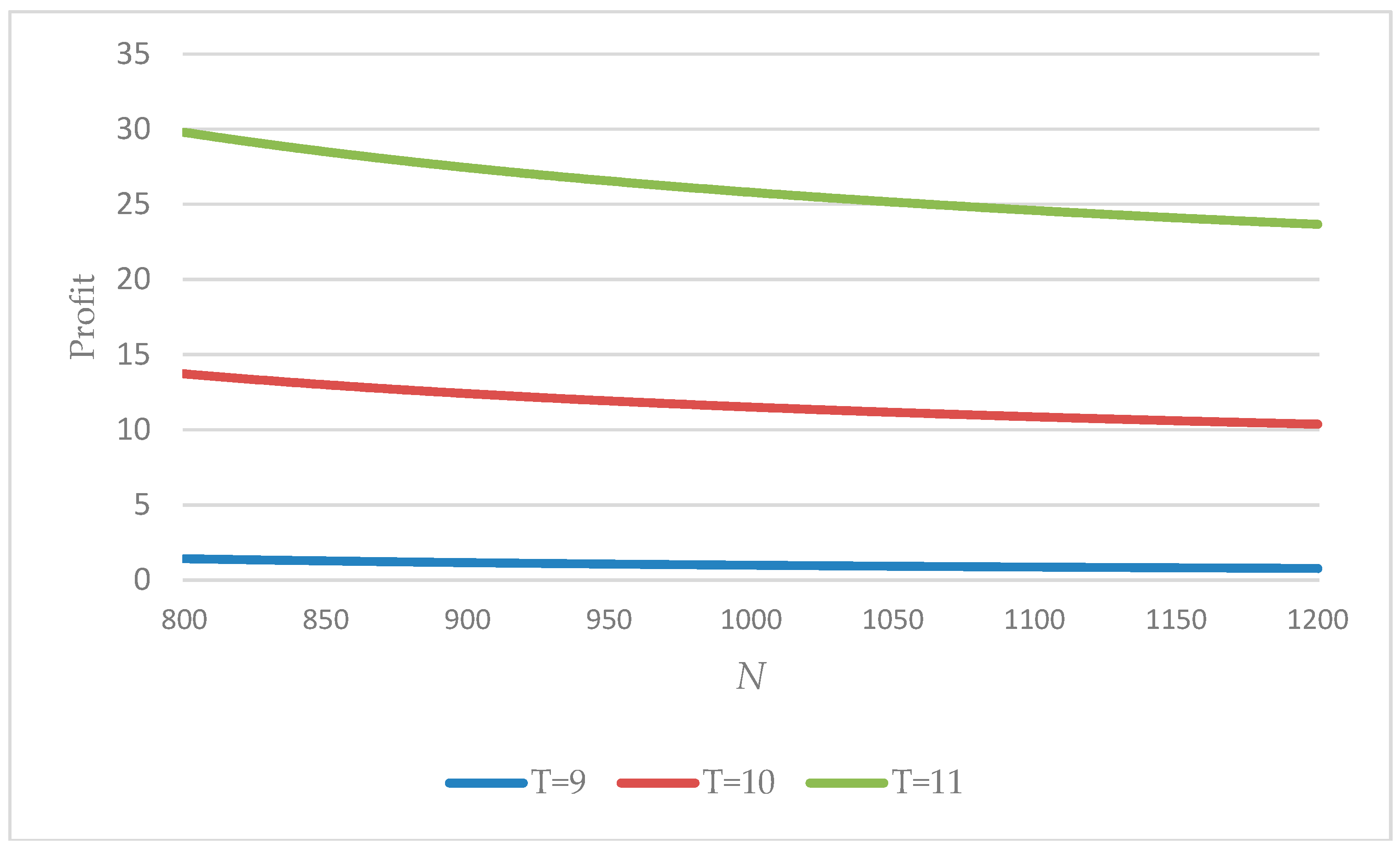
Figure 8 shows the variation of the profit when total delivery demand changes. Increased total delivery demand results in the reduction of market density, and directly affects the profit. The effect of the difference in the total working time showed similar results as in the first case. In the second case, when demand parameter is a = 300 and b = 30, the total working time must exceed 9 h per day because, as shown in Figure 8, the profit does not occur from the delivery.

5.2. Collaboration Model

We assumed that there are three express service companies, and we calculated the incremental profit from four different collaboration scenarios where the market density for each company differs: (1) 5%, 10% and 15%, (2) 5%, 5% and 20%, (3) 9%, 10% and 11%, (4) 5%, 12% and 13%. An area is selected for a collaborative last mile delivery service with express service companies. The area is divided into 10 service regions according to regional attributes, which are shown with the demand of each company in

Table 4. Data for companies A, B, and C.

Service Region	Last Mile Delivery Demand Amount
	A	B	C
1	45	90	135
2	43	86	128
3	42	83	125
4	41	82	123
5	40	79	119
6	37	75	112
7	36	72	108
8	35	70	105
9	34	67	101
10	33	66	99

,

Table 5. Last mile delivery time according to regional attribute.

Service Region	Time Shape	Market Density
		0.05	0.1	0.15	0.25	0.3
1	14.4	4.84	4.30	3.79	2.88	2.48
2	17.3	5.81	5.16	4.55	3.46	2.98
3	19.2	6.46	5.73	5.06	3.85	3.31
4	20.2	6.78	6.02	5.31	4.04	3.48
5	22.1	7.43	6.59	5.81	4.42	3.81
6	25.9	8.72	7.74	6.83	5.19	4.47
7	28.8	9.69	8.60	7.58	5.77	4.97
8	30.7	10.33	9.17	8.09	6.15	5.30
9	33.6	11.30	10.03	8.85	6.73	5.80
10	35.5	11.95	10.61	9.35	7.11	6.13

and

Table 6. Unit delivery cost according to regional attribute.

Service Region	Unit Delivery Cost			Unit Delivery Cost after Collaboration
	A	B	C	C2 (25%)	C1 (30%)
1	1.43	1.31	1.21	1.02	0.93
2	1.63	1.49	1.36	1.14	1.04
3	1.76	1.61	1.47	1.22	1.11
4	1.83	1.67	1.52	1.26	1.14
5	1.96	1.79	1.63	1.34	1.21
6	2.23	2.03	1.84	1.50	1.35
7	2.43	2.21	2.00	1.62	1.45
8	2.57	2.33	2.10	1.70	1.52
9	2.77	2.51	2.26	1.82	1.62
10	2.91	2.63	2.37	1.90	1.69

. The tables respectively show last mile delivery time and unit last mile delivery cost for each company according to the regional attributes. Time shape values for each region are obtained by using the last mile delivery time function of market density and actual average delivery time. Assuming that each delivery service worker’s income is constant regardless of the number of units, the delivery costs are calculated. We also assumed that daily working hours are eight hours, and transaction time per delivery order is two minutes. C1 and C2, shown in the last two columns in Table 6, represent the delivery cost after collaboration and mandated delivery costs. In the first case, by considering current market shares of each company, the lower bound and upper bound of selected service regions are defined as 1 and 3 for company A, 3 and 5 for company B, and 5 and 7 for company C. Applying Chung et al.’s procedure to the collaboration model with Table 4, Table 5 and Table 6, we can obtain the optimal solution based on max-min criterion using Excel Solver, which is shown in

Table 7. Optimal solution for max–min criterion (A = 5%, B = 10%, C = 15%).

Region	1	2	3	4	5	6	7	8	9	10
${\mathit{x}}_{\mathit{A}\mathit{j}}$	0	0	0	0	0	0	0	0	1	1
${\mathit{x}}_{\mathit{B}\mathit{j}}$	0	1	0	1	1	0	0	0	0	0
${\mathit{x}}_{\mathit{C}\mathit{j}}$	1	0	1	0	0	1	1	1	0	0

. We applied the same procedure for the rest of the scenarios and compared the results [23].

5.2.1. Collaboration Scenario 1: Market Density of Participating Companies (5%, 10% and 15%)

In regions 9 and 10, company A is selected for the last mile delivery service. Company B covers the regions 2, 4, and 5, and company C is responsible for the regions 1, 6, 7, and 8. The number of service regions for each company is 2, 3, and 5, respectively. The values of objective function of companies A, B, and C are ${\mathit{g}}_{\mathit{A}}$ = 303.5, ${\mathit{g}}_{\mathit{B}}$ = 384.1, and ${\mathit{g}}_{\mathit{C}}$ = 439.5.

5.2.2. Collaboration Scenario 2: Market Density of Participating Companies (5%, 5% and 20%)

The second scenario included the collaboration among two small-sized companies and one major company.

As shown in

Table 8. Data for company A, B, and C (A = 5%, B = 5%, C = 20%) and unit delivery cost according to regional attribute.

Region	d1	d2	d3	D (=d1 + d2 + d3)	cc1	cc2	cc3	C2	C1
	5%	5%	20%		5%	5%	20%	25%	30%
1	45	45	180	270	1.43	1.43	1.11	1.02	0.93
2	43	43	171	257	1.63	1.63	1.25	1.14	1.04
3	42	42	166	249	1.76	1.76	1.34	1.22	1.11
4	41	41	163	245	1.83	1.83	1.38	1.26	1.14
5	40	40	159	238	1.96	1.96	1.48	1.34	1.21
6	37	37	150	225	2.23	2.23	1.66	1.50	1.35
7	36	36	144	216	2.43	2.43	1.80	1.62	1.45
8	35	35	140	210	2.57	2.57	1.89	1.70	1.52
9	34	34	135	202	2.77	2.77	2.03	1.82	1.62
10	33	33	132	197	2.91	2.91	2.12	1.90	1.69

, we calculated the costs when collaboration is formed among the companies with market density of 9%, 10%, and 11%.

Table 9. Optimal solution for max–min criterion (A = 9%, B = 10%, C = 11%).

Region	1	2	3	4	5	6	7	8	9	10
${\mathit{x}}_{\mathit{A}\mathit{j}}$	0	0	0	0	0	0	0	1	1	0
${\mathit{x}}_{\mathit{B}\mathit{j}}$	0	0	0	0	0	0	1	0	0	1
${\mathit{x}}_{\mathit{C}\mathit{j}}$	1	1	1	1	1	1	0	0	0	0

shows companies A and B only cover two regions each, while company C covers a total of six regions. The profit for companies A, B, and C are ${\mathit{g}}_{\mathit{A}}$ = 91.3, ${\mathit{g}}_{\mathit{B}}$ = 91.3, and ${\mathit{g}}_{\mathit{C}}$ = 285.7.

5.2.3. Collaboration Scenario 3: Market Density of Participating Companies (9%, 10% and 11%)

The third scenario included the collaboration among three medium-sized companies.

Table 10. Data for companies A, B, and C (A = 9%, B = 10%, C = 11%) and unit delivery cost according to regional attribute.

Region	d1	d2	d3	D (=d1 + d2 + d3)	cc1	cc2	cc3	C2	C1
	9%	10%	11%		9%	10%	11%	25%	30%
1	81	90	99	270	1.33	1.31	1.29	1.02	0.93
2	77	86	94	257	1.52	1.49	1.47	1.14	1.04
3	75	83	91	249	1.64	1.61	1.58	1.22	1.11
4	74	82	90	245	1.70	1.67	1.64	1.26	1.14
5	71	79	87	238	1.82	1.79	1.76	1.34	1.21
6	67	75	82	225	2.07	2.03	1.99	1.50	1.35
7	65	72	79	216	2.25	2.21	2.16	1.62	1.45
8	63	70	77	210	2.37	2.33	2.28	1.70	1.52
9	61	67	74	202	2.56	2.51	2.46	1.82	1.62
10	59	66	72	197	2.68	2.63	2.57	1.90	1.69

shows the cost reduction when collaboration is formed and the market density increases. From

Table 11. Optimal solution for max–min criterion (A = 9%, B = 10%, C = 11%).

Region	1	2	3	4	5	6	7	8	9	10
${\mathit{x}}_{\mathit{A}\mathit{j}}$	1	0	1	0	0	1	1	1	0	0
${\mathit{x}}_{\mathit{B}\mathit{j}}$	0	1	0	1	1	0	0	0	0	0
${\mathit{x}}_{\mathit{C}\mathit{j}}$	0	0	0	0	0	0	0	1	1	0

, it can be found that five regions are covered by company A, three by company B, and two by company C. The profit for companies A, B, and C are ${\mathit{g}}_{\mathit{A}}$ = 373.9, ${\mathit{g}}_{\mathit{B}}$ = 383.6, and ${\mathit{g}}_{\mathit{C}}$ = 373.9.

5.2.4. Collaboration Scenario 4: Market Density of Participating Companies (5%, 12% and 13%)

The last scenario considers collaboration among one company with low market density and two medium-sized companies. In

Table 12. Data for companies A, B, and C (A = 5%, B = 12%, C = 13%) and unit delivery cost according to regional attribute.

Region	d1	d2	d3	D (=d1 + d2 + d3)	cc1	cc2	cc3	C2	C1
	5%	12%	13%		5%	12%	13%	25%	30%
1	45	108	117	270	1.43	1.27	1.25	1.02	0.93
2	43	103	111	257	1.63	1.44	1.41	1.14	1.04
3	42	100	108	249	1.76	1.55	1.53	1.22	1.11
4	41	98	106	245	1.83	1.61	1.58	1.26	1.14
5	40	95	103	238	1.96	1.72	1.69	1.34	1.21
6	37	90	97	225	2.23	1.95	1.91	1.50	1.35
7	36	86	93	216	2.43	2.12	2.08	1.62	1.45
8	35	84	91	210	2.57	2.24	2.19	1.70	1.52
9	34	81	88	202	2.77	2.41	2.36	1.82	1.62
10	33	79	85	197	2.91	2.52	2.47	1.90	1.69

, the reduced costs were calculated in each region after collaboration.

Table 13. Optimal solution for max–min criterion (A = 5%, B = 12%, C = 13%).

Region	1	2	3	4	5	6	7	8	9	10
${\mathit{x}}_{\mathit{A}\mathit{j}}$	0	0	1	1	1	0	0	0	0	0
${\mathit{x}}_{\mathit{B}\mathit{j}}$	1	1	0	0	0	1	1	0	0	0
${\mathit{x}}_{\mathit{C}\mathit{j}}$	0	0	1	1	1	0	0	0	0	0

shows that company A covers 3 regions, company B covers 4 regions, and company C covers 3 regions. The profit for companies A, B, and C are ${\mathit{g}}_{\mathit{A}}$ = 347.0, ${\mathit{g}}_{\mathit{B}}$ = 424.4, and ${\mathit{g}}_{\mathit{C}}$ = 367.5.

6. Discussion

6.1. Customer Service Quality

According to the LMF suggested in this paper, the change in travel time with the variation of market density can be confirmed. In other words, an increase in market density reduces the travel time, and this can eventually lead to a reduction of delivery time of the delivery service drivers.

Boyer studied how customer density and delivery window pattern affect the efficiency of last mile delivery [4]. However, a model was not proposed in this study. Instead, the study showed how customer density and delivery window patterns change last mile delivery time through simulation. In this paper, demand points in delivery area are randomly generated through GA, and this generating process was carried out 100 times for each of the experiments to obtain LMF, which is the approach that reflects a more realistic delivery process.

This signifies that the delivery carriers can handle more quantity within their total working time and increase customer service satisfaction at the same time. However, a decrease in market density means an increase in travel time and decrease in delivery quantity, which may lead to lower customer service quality.

In the previous studies, the travel time was generally calculated through delivery network design and was converted to cost values. The optimization for delivery network design has been studied for a long time. In this paper, however, we developed a last mile delivery function to calculate the travel time while considering the market density. There are studies that consider the effect of the market density in last mile delivery service, but these studies only performed simulation to achieve managerial insights. In this paper, we propose LMF and a pricing model, which can be considered as the more realistic last mile delivery pricing model.

6.2. Pricing Model

Since travel cost is obtained through LMF, it is possible to examine the effect of market density on price and profit, which satisfies the establishment of the pricing model in this paper. In addition, since the existence of the optimal solution in the pricing model is proven through differentiation, the solution approach is appropriate.

From the results of the sensitivity analysis in Section 5, we examined how the optimal price and profit change when the labor cost, daily working time, and total delivery demand in certain regions differ.

Nowadays, conflict between company and delivery workers is becoming aggravated. Delivery workers are demanding more labor costs and shorter working time while a company tries to adjust these elements to earn more profit. Other than labor cost and total working time, the variation of total delivery demand in a region affects the optimal price and profit. The numerical example in Section 5 shows that when the market density decreases, the price increases and the profit decreases. In addition to the effect of labor cost and working time, a company can use the proposed pricing model as the guideline for making better investment decision to expand the capacity of terminal facilities.

6.3. Collaboration Model

Small and medium-sized express delivery companies, who have a hard time investing, may use the proposed collaboration model to decide whether to collaborate with other companies and with which companies to collaborate.

For the collaboration model, max–min criteria is used to solve the objective function regarding incremental profit of participating companies. Although max–min criteria may result in smaller total collaboration pie, since the difference in profit allocation among the participating companies is the smallest with max–min criteria, it is the method that can raise the satisfaction of companies that participate in collaboration.

The proposed model showed that profit occurs when a terminal and delivery volume is shared through collaboration. In addition, we suggested four different types of collaboration, which considers the difference in market density of participating companies. In Section 5, the profit from collaboration showed difference depending on the market density of participating companies. Therefore, with the results from the numerical example, a company can make the right decision to find right cooperator to achieve the maximum profit.

Also, through collaboration, companies can reduce travel cost and other costs such as terminal operation cost. Most small and medium-sized companies do not earn enough profit due to big investments in building new terminals or developing new services. Therefore, the proposed collaboration model is a win–win and sustainable solution for small and medium-sized companies in the long term. In addition, collaboration among companies can solve environmental problems by reducing carbon emissions during delivery.

7. Conclusions

While the express delivery service market has been steadily increased according to rapid increase in business-to-consumer (B2C) demand, delivery service companies have to overcome more severe competition in the market. In order to survive in the competitive delivery service environment, they have made many efforts to establish several strategies such as service network optimization, efficient flow management, increased terminal productivity, etc. Nowadays, a quick response has been recognized as an index for representing customer satisfaction levels. It makes the express delivery service companies apply themselves to the last mile delivery process in a delivery service.

This study suggested pricing as well as collaboration models for increasing the competitiveness of delivery companies, based on the time-market density model. In the pricing model, a procedure for finding an optimal price to expand delivery service market was introduced. A last mile delivery time function of market density was also derived with GA-based simulation results of the traveling salesman problem with randomly generated customers. In addition, a collaboration model was proposed as another strategy against the difficult market situation to mediate service price. A multi-objective integer programming problem was developed and solved based on the max–min criterion. The applicability and efficiency of two proposed models were demonstrated through an illustrative numerical example. It will be beneficial to conduct case studies with real data collected from express delivery service companies.

The solution procedures for proposed models have limitations. In the pricing model, we mainly focused on the travel cost. By using LMF, a more realistic last mile delivery cost was calculated. However, we considered costs other than travel cost as constant value. In the real world, as market density differs other costs such as terminal operation costs can be affected. Including the total process of express delivery into the proposed model can make the suggested pricing model more realistic.

The suggested collaboration model considered incremental profit which assumed that collaboration always secures profit for participating companies. However, as shown in Section 5, in some cases, based on the market density of participating companies, collaboration does not always guarantee the satisfaction of companies. In this paper, we used max–min criteria to calculate the profit for participating companies. Max–min criteria have limitations because this is a method of calculating the minimum profit of a whole collaboration while reducing the imbalance of profit between participating companies. Other methodologies used game theory studies for more reasonable distribution of total profit to increase the satisfaction of participating companies.

In future studies, several types of demand functions of price will be considered in pricing model. In addition, we can apply our suggested time-density model and pricing model to other express delivery research to modify it, considering the expected profit from forming different types of hub network. Also, collaborations model will be developed and compared with each other under various criteria such as max-sum. Furthermore, development of fair allocation methods of coalition profit will be included in order to sustain long-term collaboration.

References

- Bae, M. Recent Trend in Korean Parcel Delivery Service Market. Available online: http://nlic.go.kr/nlic/knowInTotalDt.action?fldQuestionSeq=383&command=VIEW (accessed on 24 May 2016).
- Dolan, S. The Challenges of Last Mile Logistics & Delivery Technology Solutions. Available online: https://www.businessinsider.com/last-mile-delivery-shipping-explained (accessed on 10 May 2018).
- Boyer, K.K.; Prud’homme, A.M.; Chung, W. The last mile challenge: evaluating the effects of customer density and delivery window patterns. J. Bus. Logist. 2009, 30, 185–200. [Google Scholar] [CrossRef]
- Gevaers, R.; Voorde, E.; Vanelslander, T. Cost modelling and simulation of last-mile characteristics in an innovative B2C supply chain environment with implications on urban areas and cities. Procedia Soc. Behav. Sci. 2014, 125, 398–411. [Google Scholar] [CrossRef]
- Kim, S.; Lim, H.; Park, M. Analyzing the cost efficiency of parcel distribution networks with changes in demand. Int. J. Urban Sci. 2014, 18, 416–429. [Google Scholar] [CrossRef]
- Alibeyg, A.; Contreas, I.; Fernandez, E. Hub network design problems with profits. Transport. Res E-Log. 2016, 96, 49–59. [Google Scholar] [CrossRef]
- Zhou, L.; Wang, X.; Ni, L.; Lin, Y. Location-routing problem with simultaneous home delivery and customer’s pickup for city distribution of online shopping purchases. Sustainability 2016, 8, 828. [Google Scholar] [CrossRef]
- Hu, C.; Lu, J.; Lui, X.; Zhang, G. Robust vehicle routing problem with hard time windows under demand and travel time uncertainty. Comput. Oper. Res. 2018, 94, 139–153. [Google Scholar] [CrossRef]
- Xuefeng, W.; Fang, Y.; Dawei, L. Multi-objective location-routing problem with simultaneous pickup and delivery for urban distribution. J. Intell. Fuzzy Syst. 2018, 35, 1–14. [Google Scholar]
- Zhou, L.; Lin, Y.; Wang, X.; Zhou, FL. Model and algorithm for bilevel multisized terminal location-routing problem for the last mile delivery. Int. Trans. Oper. Res. 2019, 26, 131–156. [Google Scholar] [CrossRef]
- Felisberto, C.; Finger et, M.; Friedli, B.; Krahenbuhl, D.; Trinkner, U. Progress toward Liberalization of the Postal and Delivery Sector, 1st ed.; Springer Science + Business Media, Inc.: New York, NY, USA, 2006; pp. 249–264. [Google Scholar]
- Cebecauer, M.; Rosina, K.; Buzna, L. Effects of demand estimates on the evaluation and optimality of service centre locations. Int. J. Geogr. Inf. Sci. 2015, 30, 765–784. [Google Scholar] [CrossRef]
- Mills, E.S. Uncertainty and price theory. Q. J. Econ. 1959, 73, 117–130. [Google Scholar] [CrossRef]
- Polatoglu, L.H. Optimal order quantity and pricing decisions in single period inventory systems. Int. J. Prod. Econ. 1991, 23, 175–185. [Google Scholar] [CrossRef]
- Abad, P.H. Optimal pricing and lot-sizing under conditions of perishability and partial backordering. Manag. Sci. 1996, 42, 1093–1104. [Google Scholar] [CrossRef]
- Hong, K.S.; Lee, C. Optimal pricing and guaranteed lead time with lateness penalties. Int. J. Ind. Eng. 2013, 20, 153–162. [Google Scholar]
- Hong, K.S.; Lee, C. Optimal time-based consolidation policy with price sensitive demand. Int. J. Prod. Econ. 2013, 143, 275–284. [Google Scholar] [CrossRef]
- Ahmadi-Javid, A.; Amiri, E.; Meskar, M. A profit-maximization location-routing-pricing problem: A branch-and-price algorithm. Eur. J. Oper. Res. 2018, 271, 866–881. [Google Scholar] [CrossRef]
- Cruijssen, F.; Braysy, O.; Dullaert, W.; Salomon, M. Joint route planning under varying market conditions. Int. J. Phys. Distrib. Logist. Manag. 2007, 37, 287–304. [Google Scholar] [CrossRef] [Green Version]
- Lozano, S.; Moreno, P.; Adenso-Diaz, B.; Algaba, E. Cooperative game theory approach to allocating benefits of horizontal cooperation. Eur. J. Oper. Res. 2013, 229, 444–452. [Google Scholar] [CrossRef]
- Kimms, A.; Kozeletskyi, I. Core-based cost allocation in the cooperative traveling salesman problem. Eur. J. Oper. Res. 2016, 248, 910–916. [Google Scholar] [CrossRef]
- Wang, Y.; Zhang, J.; Assogba, K.; Lui, Y.; Xu, M.; Wang, Y. Collaboration and transportation resource sharing in multiple centers vehicle routing optimization with delivery and pickup. Knowl.-Based. Syst. 2018, 160, 296–310. [Google Scholar] [CrossRef]
- Chung, K.H.; Rho, J.J.; Ko, C.S. Strategic alliance model with regional monopoly of service centers in express courier services. Int. J. Serv. Ind. Manag. 2009, 5, 774–786. [Google Scholar]
- Ferdinand, F.N.; Chung, K.H.; Ko, H.J.; Ko, C.S. A compromised decision making model for implementing a strategic alliance in express courier services. INF. Int. Interdisciplin. J. 2013, 15, 6173–6188. [Google Scholar]
- Ko, C.S.; Min, H.; Ko, H.J. Determination of cutoff time for express courier services: A Genetic algorithm approach. Int. Trans. Oper. Res. 2007, 14, 159–177. [Google Scholar] [CrossRef]
Figure 1.
Trend for express service market in Korea [1].
Figure 2.
An example of express delivery service flow.
Figure 3.
Last mile delivery time pattern in service region during a shift.
Figure 4.
An example of last mile delivery time function of market density.
Figure 5.
Variation of the optimal price with w for different values of T (N = 800).
Figure 6.
Variation of the profit with w for different values of T (N = 800).
Figure 7.
Variation of the optimal price with N for different values of T (w = 150).
Figure 8.
Variation of the profit with N for different values of T (w = 150).