Closed Loop Supply Chain under Power Configurations and Dual Competitions

Department of Industrial Engineering, Tsinghua University, Beijing 100084, China
*
Author to whom correspondence should be addressed.
Sustainability 2018, 10(5), 1617; https://0-doi-org.brum.beds.ac.uk/10.3390/su10051617
Submission received: 10 April 2018
/
Revised: 5 May 2018
/
Accepted: 11 May 2018
/
Published: 17 May 2018
(This article belongs to the Special Issue Sustainable Supply Chain System Design and Optimization)
Abstract
:This paper investigates pricing and collecting decisions in a closed loop supply chain (CLSC) under different power configurations and dual competitions. If the original equipment manufacturer (OEM) could sell products directly and collect used products, OEM has to compete with both forward retailer and reverse collector, simultaneously, and OEM possesses different bargaining powers. Specifically, we examine the following models: (1) M1: OEM holds the first position in both forward and reverse channels; (2) M2: OEM holds the first (second) position in the forward (reverse) channel; (3) M3: OEM holds the second position in both channels. We conduct a systematic comparison of forward competition, reverse competition and dual competitions across the above models. From the perspective of the entire supply chain, the outcome of model selection hinges on the extent of competition. If the competition is sufficient, two forward leaders will engage in a price battle which results in great losses for both. Then M1 is preferred. Otherwise, M3 outperforms.
1. Introduction
In recent years, the economic and environmental benefits of recovering obsolete products have been widely recognized in literature and practice. Under some legislation based on extended producer responsibility (EPR) about end-of-life (EOL) products, more and more original equipment manufacturers (OEMs) build their own reverse channels to collect used products [1]. For instance, more than 65% of the population of the U.S. is now covered by state e-waste recycling laws [2]. Latest research on channel management of CLSCs also suggests that EPR policies require both the manufacturer and the consumer to bear environmental charges over the product’s life cycle [3]. Accordingly, Atasu and Subramanian [4] compare the implications of collective/individual producer responsibility (CPR/IPR) on manufacturers’ design for product recovery choice and profits. In practice, many OEMs add additional recycling channels in order to collect enough quantities of EOL products. For instance, OEM and an independent collector share producer responsibility, collectively. Kodak competes with collectors to collect single-use cameras [5,6]. Another recycling channel will inevitably cause channel competition between reverse members [7]. Moreover, channel leadership might have influence on the competition and performance [8].
On the other hand, with the rapid development of Internet, the supply chain system no longer consists of a single traditional channel, and many manufacturers set up direct channel to sell products online, such as Apple, IBM, Hewlett-Packard [9,10]. This new business mode can seriously lead to forward competition so that OEM has to compete with both forward retailer and reverse collector, simultaneously [11]. Then channel leadership affects not only reverse competition, but also forward channel performance. To our knowledge, there is little research considering the impact of both power configuration and dual competitions on closed loop supply chain (CLSC) management.
In terms of OEM’s dual power configuration, we establish four models as follows: the centralized model (M0), a model where OEM holds the leader position in both forward and reverse channels (M1), a model where OEM holds the first (second) position in forward (reverse) channel (M2), and a model where OEM are the follower in both channels (M3). We refer the reader to Figure 1 in Section 3 for further illustration of the power configurations M0–M3. From the viewpoint of OEM, we aim at addressing the following open research questions: (1) How do different power configurations influence forward competition, reverse competition, and dual competition? (2) Under OEM’s different positions in the power configuration, how do dual competitions influence the performance of CLSC? (3) Among M1, M2, M3, which one is the best model from total CLSC’s perspective?
Our contribution in this paper lies in the following three aspects. First, we provide a systematic comparison of forward competition, reverse competition and dual competitions between four models in the order of OEM’s power configuration. Secondly, we consider the joint effects of dual channel competitions and OEM’s power configurations on system’s performance. Specifically, it notes that if reverse channel is led by the collector, he will take the same perspective as does the whole CLSC, no matter who leads forward channel. From the viewpoint of extended producer responsibility (EPR), if reverse competition is not fierce, CPR policy is preferred; otherwise, IPR policy is better. Thirdly, the selection of the best mode depends on dual competitions. If the competition is fiercer enough, two forward leaders will engage in a price battle which results in great losses for both. Then M1 is preferred; otherwise, M3 outperforms. Besides, dual competitions also generate a substitution effect.
We organize the remaining of this work as follows. We review the literature in the next section. We describe the model notations and assumptions in detail in Section 3, and in Section 4 we present four models in the order of OEM’s power configuration, i.e., M0, M1, M2, and M3. We provide a systematic comparison of forward competition, reverse competition and dual competitions about the above mentioned four models in Section 5. We finally conclude this work in Section 6. All proofs of this paper are presented in the Appendix A.
2. Review of the Literature
There is vast amount of research papers on closed loop supply chain [12,13,14]. We mainly focus on three streams of literature., i.e., forward competition, reverse competition, and channel power configuration, each of which is reviewed as follows.
First, literature about dual-channel forward competition can be sorted into two categories. On the one hand, it is intuitive the competition exists between remanufactured and new products provided by remanufacturers and OEMs, and whether the firm charges the same price for the two types of products is a key assumption. If there is no distinction between the new and remanufactured product, Ferrer and Swaminathan [15,16] develop monopoly and duopoly competitions in two periods, multiple-period, and infinite-horizon models, and analyzed the equilibrium prices and quantities in price competition. Surprisingly, they identify the optimal policy is not necessarily monotone in remanufacturing savings. If the remanufactured product differs with the new one, Ferguson and Toktay [17] demonstrate that a firm may choose to remanufacture or preemptively collect its used products to deter entry, even when the firm would not have chosen to do so under a pure monopoly environment. Webster and Mitra [18] examine the effect of legislations and regulations on remanufacturing activities. In this study, we consider the case where the remanufactured product is not distinguishable from the new product—therefore the firm could charge them the same price.
On the other hand, more and more OEMs add additional their own online channels in practice, then a few researchers address the direct versus retail competition. Balasubramanian [19] reports competition between direct marketers and conventional retailers, and they find that each retailer competes against the remotely located direct marketer, rather than against neighboring retailers. Cattani et al. [20] focus on the coordination opportunities that arise when a firm participates in both a traditional channel and an online channel. Further, Cattani et al. [21] finds if the Internet channel is of comparable convenience to the traditional channel, then the manufacturer has remarkable incentive to abandon the equal-pricing policy, which poses great challenge to the traditional retailer. In the spirit of the studies above, we assume the forward competition exists between direct and retail channels. But different from the literature in this stream, our model also accounts for power configurations in the channel and its effect.
Second, there are numerical studies on reverse channel competition. Savaskan et al. [22] compare manufacturer collecting, retailer collecting and collector collecting in a single channel. This excellent work has inspired vast amount of papers further examining the reverse channel choices. Together with reverse channel, take-back laws based on EPR are considered. Likewise, it is possible for the implementations of collective producer responsibility (CPR) owing to dual-channel collection. On the one hand, from CPR’s perspective, Atasu and Subramanian [4] compare collective and individual producer responsibility, and conclude that CPR may distort competition and allow free-riding, which may cause the manufacturer’s preferences for IPR or CPR to differ. Accordingly, Nie et al. [23] examine two strategies for CPR, namely, the financial sharing (FS) and the physical sharing (PS), using the model with no CPR as a benchmark. Shi et al. [24] separately inspect retailer collection, manufacturer collection and third-party collection with CPR. Furthermore, Gui et al. [25] revisit the assertion that CPR provides inferior design incentives compared to IPR in a supply chain network setting. Unlike above studies, we take into account the impact of power distribution in reverse and forward channels on the CPR policy.
On the other hand, from the perspective of dual reverse channel, Huang et al. [7] investigate optimal strategies of CLSC with dual recycling channel, where the retailer and third party competitively collect used products. They find that dual recycling channel dominates the single recycling channel only when the competition in recycling is not strong. Hong et al. [26] study three forms of dual-channel collection, i.e., OEM & retailer, OEM & collector, and retailer & collector. In our setting, the reverse competition exists between the collector and OEM. That is, OEM in our study could collect the used products directly. Different from extant works in reverse channel competition, our study takes not only the competition between the collector and OEM into consideration, but also the comparison of CPR and IPR.
The third stream related to our work explores channel leadership in CLSCs. Karakayali et al. [27] analyzes remanufacturer-driven and collector-driven decentralized collection and operations for the end-of-life products in the durable goods industry. Choi et al. [8] examine the performance of different CLSC under different channel leadership, and find that the retailer-led model gives the most effective CLSC. Maiti and Giri [28] investigate the effect of channel power structures on different CLSC policies, finding that retailer-led decentralized policy is more acceptable among the decentralized policies. Gao et al. [29] study the pricing and effort decisions in a CLSC under various power configurations and the results show that with dominant power shifting from the manufacturer to the retailer, the retailer’s profit always increases and the manufacturer may also benefit when the effectiveness of collection effort in demand expansion is large enough. Compared with our work, the above studies do not incorporate dual competitions on CLSC. That is, there exist competitions in both reverse and forward channel. Since the OEM in our study participates in both reverse collecting and forward selling, the OEM’s positions in distinct competitions determine the power configuration.
Our study is closely related to the previous work by Zheng et al. [11], which investigates pricing and coordination decisions in dual-channel CLSCs in the presence of different power structures and forward channel competition. In lack of reverse competition, Zheng et al. [11] only allows the supply chain to be led by a single party, i.e., either the retailer, the manufacturer, or the collector. In contrast, our work incorporates competition in the reverse channel which enables the analysis of power configuration in both forward and backward supply chains.
3. Assumptions and Notations
3.1. Notations
The symbols used in this paper are summarized in Table 1.
3.2. Assumptions
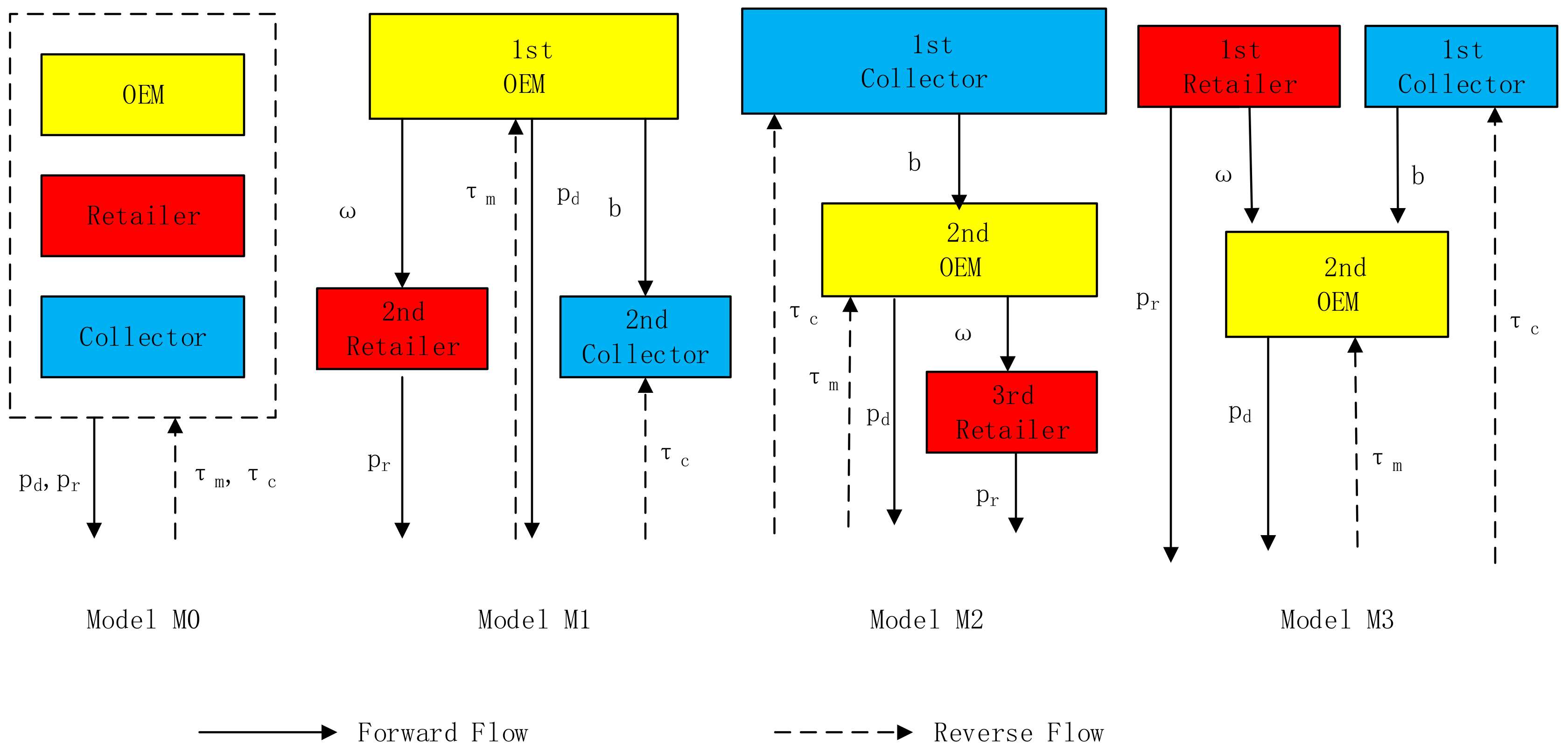
We consider dual competition CLSC which consists of a OEM (he), a retailer (she) and a collector. The OEM wholesales the product through the retailer’s channel at a price w, and also distributes the product through his owned direct channel at a price . The OEM repurchases used products from the independent collector with paying a transfer price b for each unit, and also collect the used products by his owned reverse collection channel. From the perspective of OEM, we depict the competition power configuration. Facing with any competition, OEM holds two power positions. Under dual competitions, there exist three cases for OEM. As shown in Figure 1, OEM holds both first positions in both forward and reverse channels (Model M1); OEM holds first (second) position in forward (reverse) channel (Model M2); OEM holds both second positions (Model M3). Since there exists no power position in the centralized case, the model is expressed as Model M0. Superscript j will take values M0, M1, M2 and M3, which will denote centralized case, both first power positions, one first and one second position, and both second positions, respectively.
For brevity, the following modeling assumptions are considered.
- (1)
- All players in our model are assumed to be risk-neutral and profit seeking, and have access to the same information. And the CLSC decisions are considered in a single-period setting.
- (2)
- There is no distinction between the new and remanufactured product, i.e., they are priced same.
- (3)
- Manufacturing a new product from a used product is less costly than using raw materials, i.e., . Following Savaskan et al. [22], we use to denote the unit cost saving from product remanufacturing.
- (4)
- Referring to Ingene and Parry’s approach (Ingene and Parry [30]), the retailer and OEM face a demand pattern given bywhere is the quantity of product sold by the retailer (OEM), and is the retail (direct) price charged by the retailer (OEM), . Parameter denotes forward channel substitutability. That is, could be regarded as the forward competition intensity between reverse/forward members. If , the products are completely monopolistic. As increases, competition in the forward channel becomes more intense. If approaches 1, both products are purely substitutable.
Then in our setting, the demand depends on three elements, its own selling price, the rival’s selling price and the competition intensity. In fact, the demands for both direct and retail channels are generated from a utility function for a representative consumer . Similar utility function has been wildly adopted in the literature (Zheng et al. [11], Yan et al. [31]).
(1) Following Huang et al. [7], the collector’s and OEM’s investment cost, , can be rewritten as the function of return rates:
where refers to the competition intensity between the collector and OEM. The parameter C is a scaling parameter, the exchanging coefficient between the return rate and investment on recycling. To ensure that all of the optimal values are positive, C is assumed to be sufficiently large. The parameters denote the return rate of the OEM, collector, and total CLSC, respectively. Then investment cost is the function of its own return rate, its competitor’s return rate and reverse competition intensity.
4. Model
In this section, we establish four dual-competition CLSCs models and solve model equilibrium solutions for comparisons completely.
4.1. Model M0
We begin by analyzing Model M0, the centralized model, which provide a benchmark for us to compare with the subsequent three decentralized models. In Model M0, there exists no power configuration and all players form a strategic alliance to determine channel prices , , and return rate , .
The optimization problem of Model M0 is
Solving the above problem, the optimal prices and return rates are shown in Theorem 1.
Theorem 1.
When the parameter C satisfies , the profit function (3) is concave, then ,.
From the total CLSC’s perspective, the baseline equilibrium results are shown in Theorem 1. In the forward channel, retail price is equal to the direct price; while in the reverse channel, OEM’s return rate is in line with the collector’s.
4.2. Model M1
In Model M1, OEM holds the first power position under both forward and reverse competition. The sequence of the event is as follows. First, OEM first determines . Second, the retailer sets , and the collector determines . Hence, the optimization problem of Model M1 can be stated as
We show the optimal transfer price, optimal retail/direct price, optimal wholesale price, and optimal collector’s/OEM’s return rate in Theorem 2.
Theorem 2.
In the Model M1, the optimal decisions are given by , , , , .
4.3. Model M2
Compared with Model M1, in Model M2, OEM never holds the first power position under both flows. Instead, he just plays the leader in one flows while he holds the second position in other flows. In the dual competition, the retailer and the collector will both be possible to act as the channel leader. Since this study focuses on CLSC, we take the collector-led case for the example and the retailer-led case is likewise. Under the reverse competition, OEM plays the follower while he acts as the leader under the forward competition. The sequence of the event is as follows. First, the collector determines Second, OEM first determines Finally, the retailer sets Hence, the optimization problem of Model M2 can be stated as
From Equations (7)–(9), we can derive the optimal results in Theorem 3.
Theorem 3.
In the Model M2, the optimal decisions are given by , , , .
4.4. Model M3
In Model M3, OEM holds both second power position under dual competition. Then the collector and retailer both act as the leader in respective competition. The sequence of the event is as follows. First, the retailer sets , and the collector determines , . Second, OEM first determines . It notes that first power of both sides is symmetric, and to ensure OEM’s participation, OEM’s profit is always at least zero. Hence, the optimization problem of Model M3 can be stated as
The equilibrium solutions of Model M3 are shown in Theorem 4.
Theorem 4.
In the Model M3, the optimal decisions are given by , , , , , where .
5. Comparison of the Four Dual-Competition CLSCs
5.1. Reverse Competition
First, we investigate the transfer price, which determines how to divide the reverse channel. Second, we analyze the return rate, which can be viewed as the performance of reverse channel, meanwhile, we also focus on the optimal collective proportion between collective members in order to compare IPR with CPR. Moreover, the parameters are set as follows: , , , and these values will apply throughout the numerical analysis. In Figure 2, Figure 3, Figure 4, Figure 5, Figure 6, Figure 7, Figure 8, Figure 9, Figure 10 and Figure 11, .
5.1.1. Comparison of Transfer Price
Proposition 1.
The optimal transfer prices satisfy the following relationship: .
First, the optimal transfer price is lowest in M1 because it is offered by OEM, not the collector. Clearly, since the transfer price is lower than the cost saving from the remanufacturing, OEM could also benefit from the collector’s return rate. Also, if the transfer price is offered by the collector, the transfer price in M3 will be lower than in M2. When the collector leads the channel in M2, there are a first follower and a second follower in the three-echelon CLSC. When both the collector and retailer lead the channel in M3, there is only one follower. It implies that reverse competition is affected by the forward power configuration.
Second, transfer price plays a key role in the reverse channel. Total production cost will increase in the transfer price. Without restraints of the retailer in M3, the collector, as the single leader in M2, will offer the largest transfer price so that the total production cost is the largest. Meantime, OEM’s forward channel profit has also been extracted and forward channel is also distorted.
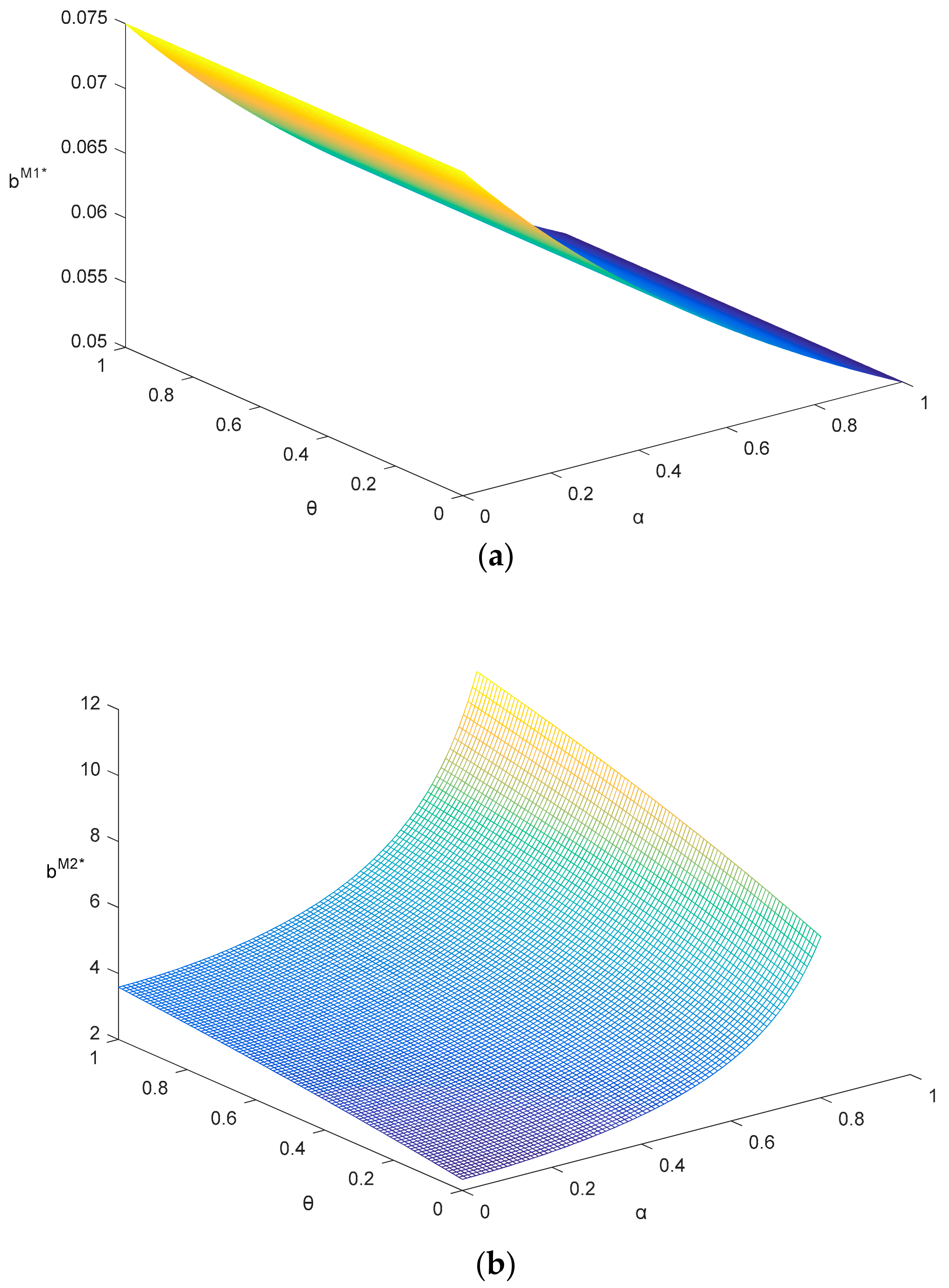
By Figure 2, we can analyze the impact of dual competition intensities on the transfer price. If OEM leads the reverse channel in M1, transfer price decreases with . Intuitively, as the competition increase, decreasing transfer price can not only strengthen their own competitiveness, but also beat the collector. However, if the collector is the leader, he will behave analogously as does OEM in Figure 2b. Compared with transfer price irrelevant to in M1, will also increase in . Since OEM compete in both channels, the collector raises the transfer price in order to beat OEM again as forward competition intensity increases. Then when is larger, OEM will be exploit from both channel.
5.1.2. Collective Producer Responsibility (CPR) vs. Individual Producer Responsibility (IPR)
Compared with single reverse channel, reverse competition between the collector and OEM indicates double collection channel. From the perspective of extended producer responsibility (EPR), single channel can be regarded as individual producer responsibility (IPR) while double reverse channel implies collective producer responsibility (CPR). For IPR, EOL products could be collected by either OEM, or the collector. For CPR, it is essential to discuss the responsibility sharing between both members. Moreover, this part focuses on how the power configuration and competition intensity affect the responsibility sharing. Besides, we explain the advantage of CPR firstly.
On the one hand, from CLSC’s perspective, the profit under IPR and CPR is shown as follows:
Given the same condition, the profit of forward channel and the revenue of reverse channel under different policies are the same, except for reverse channel cost.
By the comparison, we can know if , i.e., no competition, CPR outperforms IPR. As goes up, the advantage of CPR decreases. If , the progress is even equal to .
On the other hand, from the perspective of OEM, his profit under CPR is composed of four parts, forward retail channel, forward direct channel, reverse collector’s channel, and reverse own channel, which is as follows:
Compared with IPR policy, OEM could benefit from his own reverse channel in addition under CPR. Likewise, as goes up, his profit of own reverse channel goes down, i.e., the advantage of CPR decreases.
Overall, if reverse competition is not fierce, CPR policy is preferred; otherwise, IPR policy is better. Intuitively, if both sides compete against each other, it is impossible to share the recycling market collectively. Next, Proposition 2 shows how the responsibility sharing is influenced by the power configuration and competition intensity.
Proposition 2.
The optimal collective proportions are , where .
Proposition 2 indicates the optimal collective proportion only depends on the reverse power configuration. To be specific, the proportion is more than 1 and only depends on the reverse competition intensity if OEM leads the reverse channel. However, if the collector is the leader, the optimal proportion remains at 1 which is consistent with that in Model M0. That is, his return rate is equal to OEM’s. Namely, to optimize the performance of reverse channel, the perspective of the collector is consistent with that of CLSC, no matter who leads forward channel. Compared with the collector-led model, OEM’s return rate is higher if he is the leader. Because he can take control of the forward channel to affect the reverse channel. According to Proposition 2, we can compare the return rates. Before, we first introduce Corollary 1 to explain the relationship between return rate and sale quantities.
5.1.3. Comparison of Return Rate
Corollary 1.
Return rate is increasing in the total quantities.
Return rate includes OEM’s return rate, collector’s return rate and total return rate. By Corollary 1, all kinds of return rates are all increasing in the total quantities. Since the reverse channel is determined by the return rate, Corollary 1 implies the reverse channel depends on the forward channel. And the larger forward channel leads to the larger reverse channel.
Proposition 3.
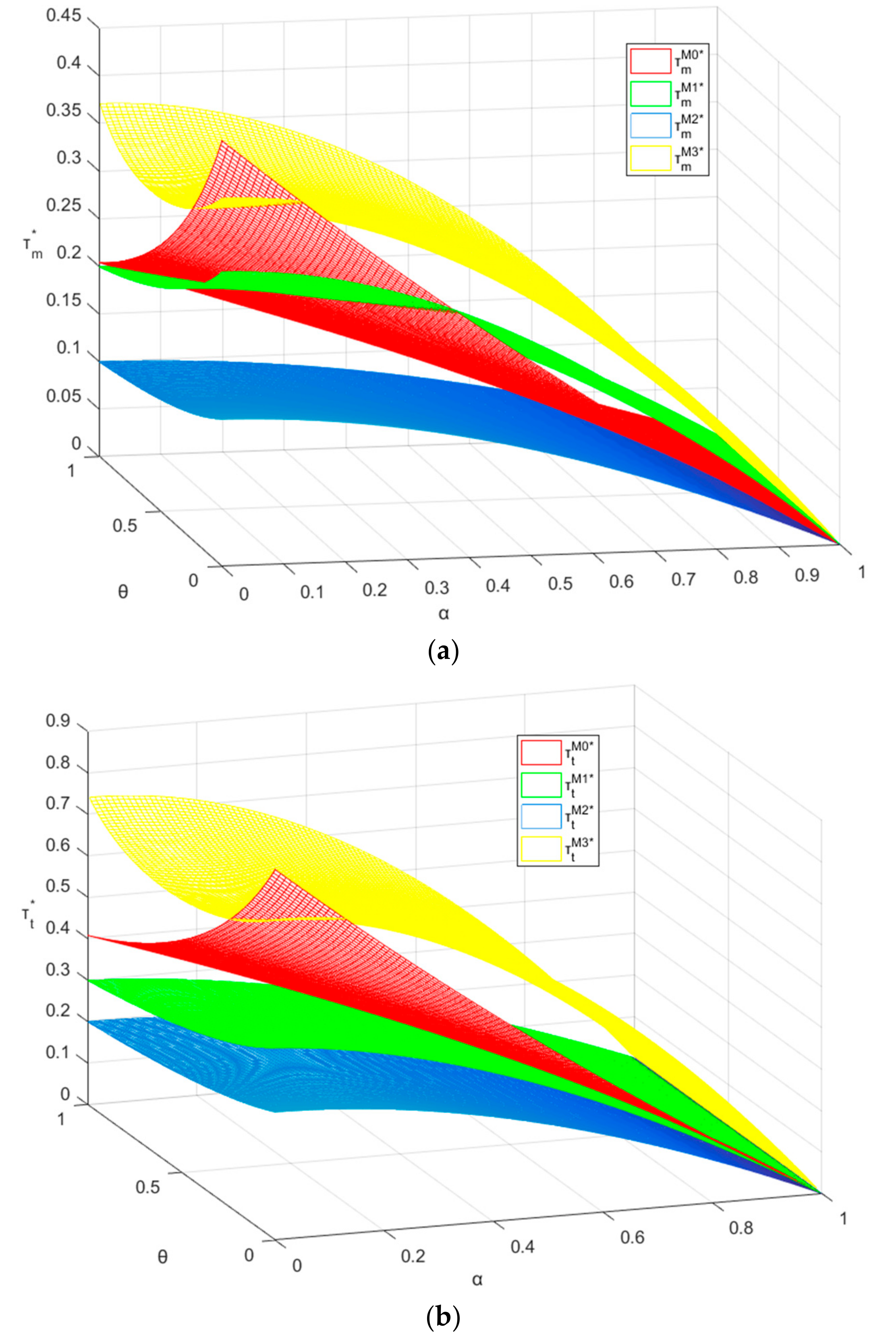
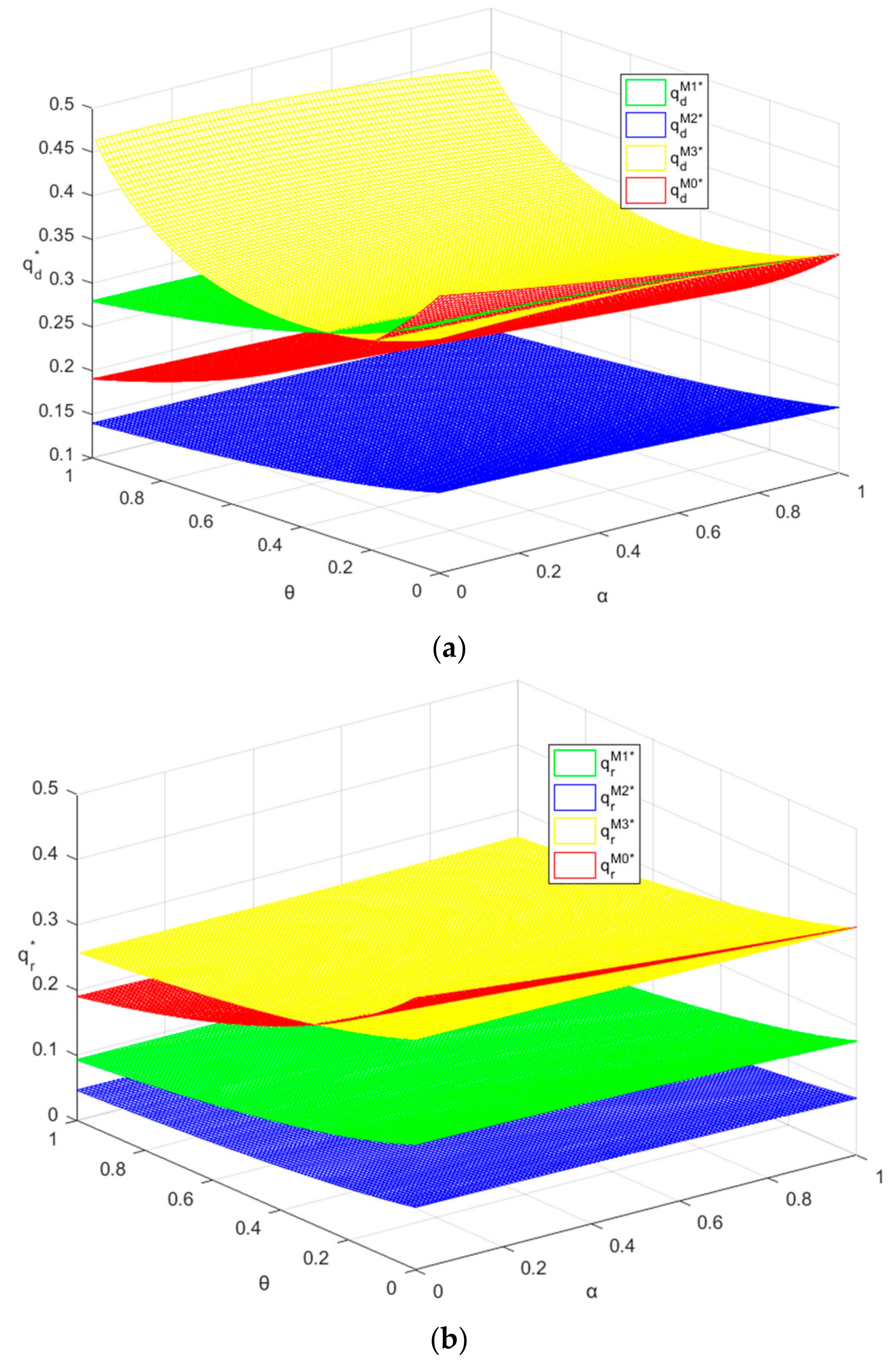
(i) The optimal collector’s return rates satisfy . (ii) The optimal OEM’s return rates are related as follows:. If and only if and are larger,;if and only if and are smaller,.(iii) The optimal total return rates are related as follows:.
Proposition 3 shows the relationships of return rate between different models. Intuitively, is the smallest if the leader is OEM. Otherwise, the optimal collective propositions in other three models are all 1:1. Namely, the comparison of the collector’s return rate is also consistent with that of OEM’s. One of the decentralized models outperforms the centralized model in the return rate, while the other one underperforms. Combined with Proposition 1, if the collector is the unique leader in CLSC, his main means for raising his profit is to increase the transfer price. However, if the collector has to share the leadership with the retailer in M3, rising up the transfer price might be restrained by the behavior of the retailer. Then improving the performance of reverse channel is also significant for the collector. Hence, the collector’s return rate is highest in M3. This indicates all the aspects of reverse channel are influenced by the power positioning in the forward channel.
By Proposition 3(ii), the relationship between is consistent with 3(i), but the ranking of is influenced by the dual competition intensities. First, from the perspective of OEM, he can benefit from his own return rate. When OEM leads the forward channel, he will expand the total quantities by Corollary 1. Therefore, OEM has more incentives to expand his own return rate. Figure 3a illustrates the impact of both on OEM’s return rate. If dual competitions are not fierce, is the largest. As rise in value, OEM’s return rates are all decreasing. Meantime, will first be exceeded by , and then be lower than . Hence, compared with centralized model in M1, with the increase of competition intensities, no matter who leads the reverse channel, he will reduce the return rate slowly so as to maintain his performance of reverse channel.
Proposition 3(iii) lists the comparison of total return rate between four models. The total return rate can be viewed as the performance of reverse channel. It is determined by OEM and the collector. By Proposition 3(iii), several interesting conclusions could be obtained. First, is the largest, while is the smallest. This implication is that the performance of reverse channel is affected by the forward power configuration. Since the collector is farther from the market, he has to tradeoff between higher transfer price and better total performance if he leads the reverse channel. If he leads the whole CLSC, he prefers higher transfer price. Otherwise, larger total return rate is better. Second, by Figure 3, as goes up, all the return rate decrease. Namely, the performance of reverse channel is worse off and even decreases to zero. In the worst case, reverse channel will be closed.
5.2. Forward Competition
Next, we give some comparative results between these models.
Proposition 4.
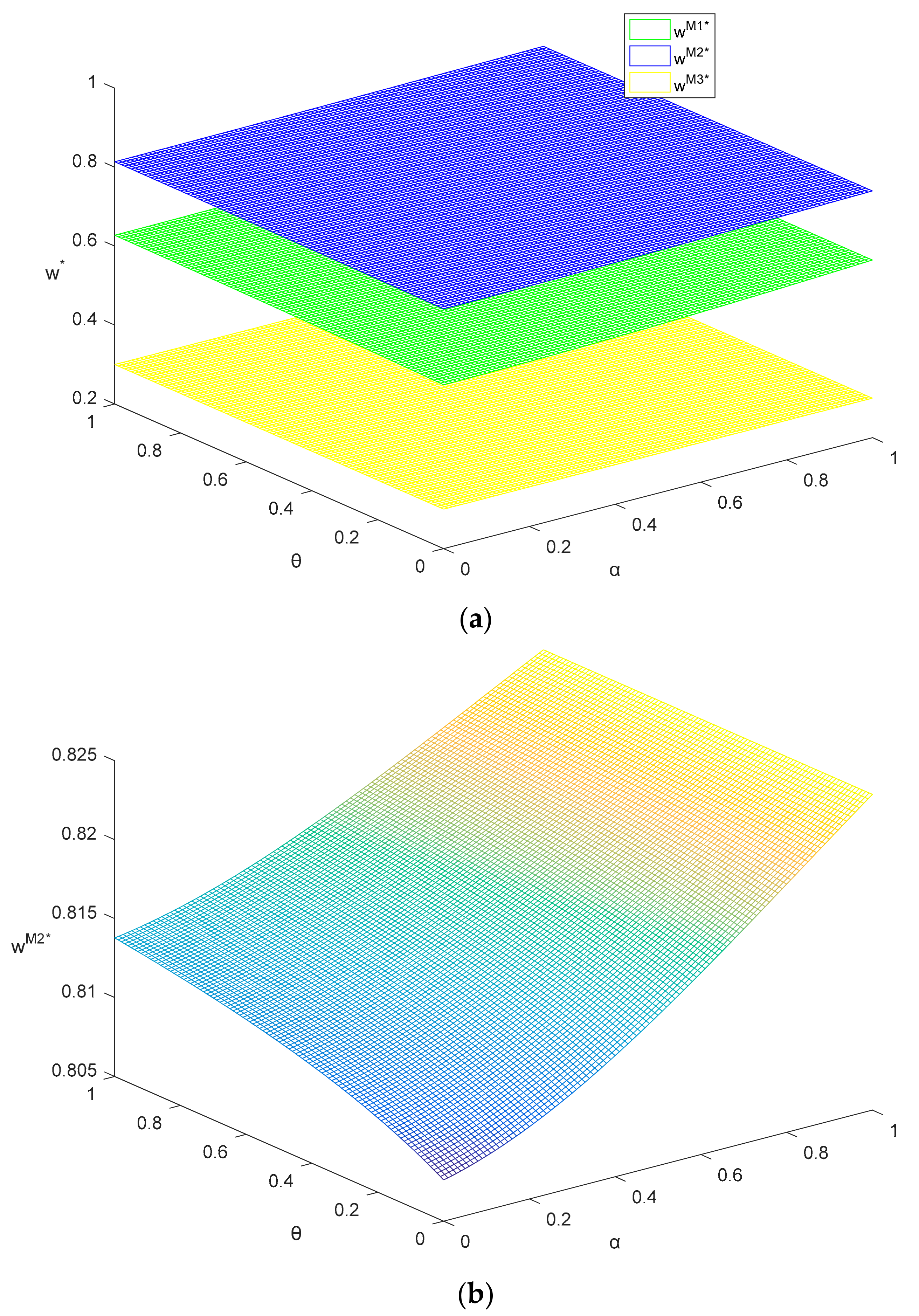
The optimal wholesale prices satisfy .
It is intuitive that the wholesale price is smallest when the retailer leads the forward channel because he has strong incentive to cut the wholesale price. Furthermore, if OEM is incapable of selling the products directly, he might get nothing in the forward channel since the wholesale price offered by the retailer is even equal to OEM’s total cost. The wholesale price is highest in M2 since the forward channel in M2 is affected by reverse competition. Faced with highest transfer price, OEM has to raise the wholesale price. Compared with has been distorted further.
Figure 4 illustrates the wholesale price. By Figure 4a, we can know the wholesale price lies on different levels when OEM holds different configurations. Namely, from the perspective of the retailer, his cost varies in different model. And the gap between different levels is so large that the ranking of the wholesale price is independent of competition intensities in both channels, even though every wholesale price is affected by both . We take for the example. First, the wholesale price is offered by OEM. As goes up, he will raise the wholesale price in order to increase the retailer’s cost. Then his competitive advantage has been strengthened while the retailer’s has been weakened. It notes that as goes up, the wholesale price is also increasing. Because the transfer price offered by OEM increases sharply with the increase of , then OEM has to charge higher wholesale price from the retailer. Namely, the reverse competition affects the forward channel.
Proposition 5.
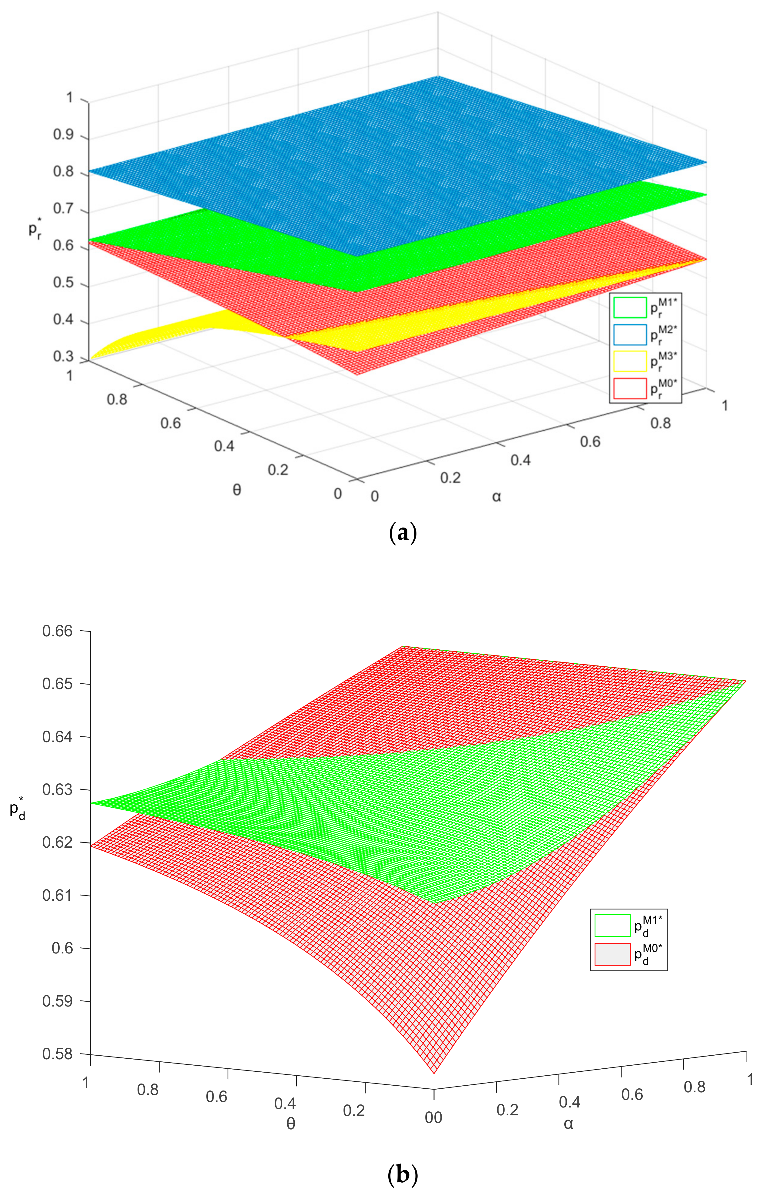
(i) The optimal retail prices are ordered as follows: . If and only if and are smaller, . (ii) The optimal direct prices are ordered as follows: . If and only if and are larger, ;if and only if and are smaller, .
By Proposition 5(i), it is intuitive that the optimal retail price is lowest in Model M3 given his cost, i.e., the wholesale price is lowest. Besides, the wholesale price can be viewed as the cost of the retailer’s forward channel. Then the ranking of retail price between is consistent with that of wholesale price. Similar to Proposition 3, we find that retail price in M-(R-)led model outperforms (underperforms) that in the centralized model.
By Figure 5a, if both competitions become fiercer, the retailer has a full control over the retail channel in Model M3 and he has a strong incentive to charge a lower retail price so as to increase the retail channel competitiveness. Under decentralized models, i.e., M1, M2, M3, retail price goes down as competition increases. However, the retail price in the centralized model increases with . Because the integrated firm sets identical channel prices to maximize total quantities.
Proposition 5(ii) reveals the comparison of optimal direct prices. If OEM leads the forward channel, the wholesale price, offered by him, will be equal to the direct price. If unequal, the retailer will choose the lower one. Then OEM faces up with the tradeoff between lower direct price and higher wholesale price. By Proposition 5(ii), the direct price in Model M2 is higher than it in Model M1. If the forward channel is led by the retailer, OEM’s direct price will not be constrained by the wholesale price. The wholesale price offered by the retailer in M3 is so low that has the same ranking of direct price.
It is also interesting to observe that optimal direct price in M0 could be regarded as one boundary. Below the boundary, the retailer holds the first position; otherwise, OEM leads the forward channel. By Figure 5b, if both competition intensities become increased, direct price grows. Faced up with the tradeoff between decreasing direct price and increasing the retailer’s cost, the latter impact dominates. However, if the retailer leads the channel, direct price in M3 goes down. OEM has strong incentive to charges a lower direct price so as to increase the direct channel competitiveness. Since the cost gap between two sellers is not that large in M3, the direct price drops sharply as the competition grows.
To sum up, when transfer price in M2 is adequately high, all the forward prices, including wholesale price, direct price, and retail price, are all highest. Second, as the competition grows, the retailer prefers to cut down the price, while OEM’s power configuration determines his behavior. If he holds the first position, he chooses to raise his price; otherwise, he has to cut his price. Besides, if OEM leads the forward channel, the cost gap between both forward members is so large that their competition is not in the same level. However, if the retailer takes control of wholesale price, his cost will be close to OEM’s. Then they will engage in a price battle. According to Proposition 4, we can get Corollary 2, which will further illustrate the final outcome of this price battle.
Corollary 2.
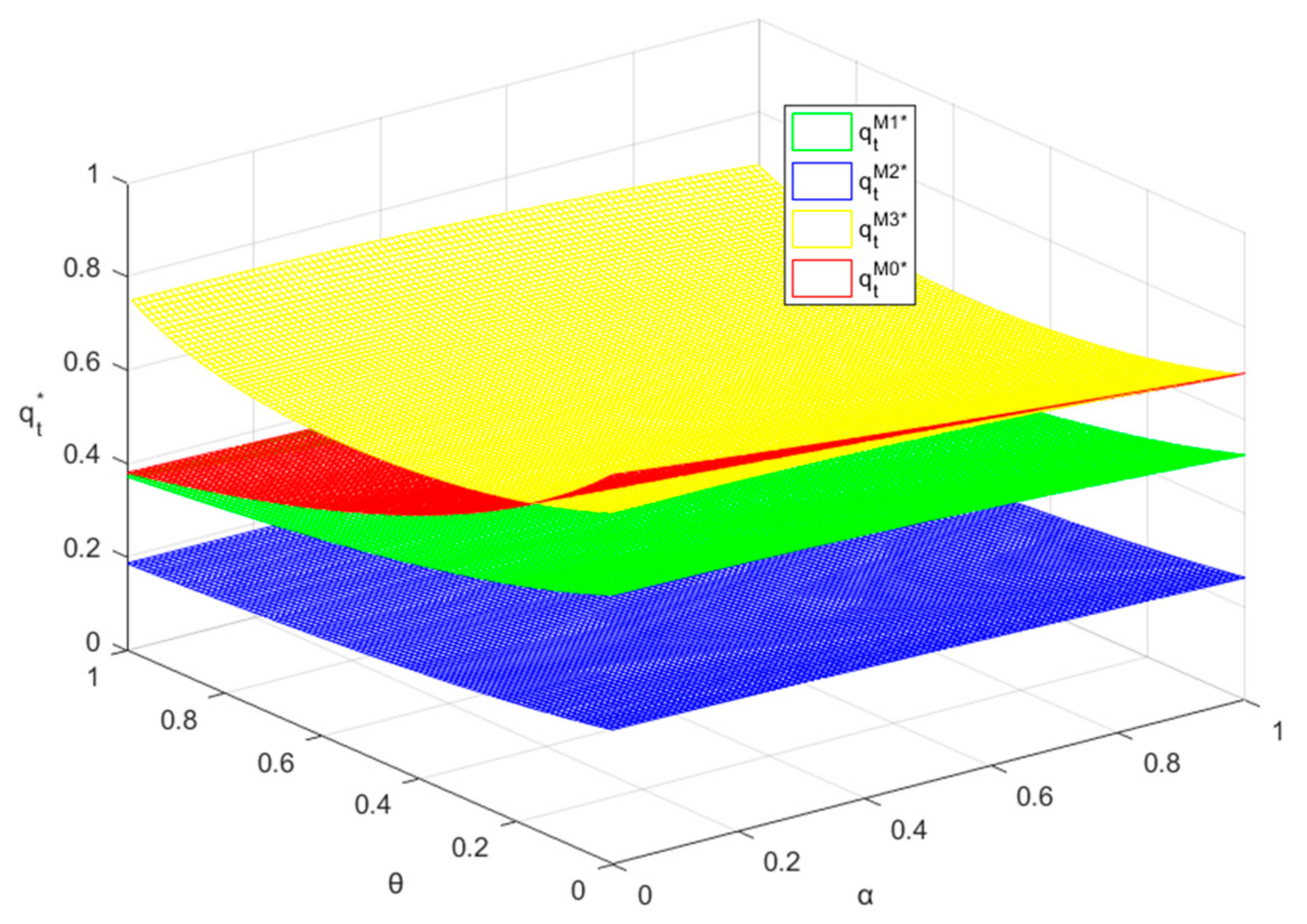
(i) The optimal quantities of the direct channel satisfy . If and only if and are smaller, ; (ii) The optimal quantities of the retail channel satisfy ; (iii) The optimal total quantities satisfy . If and only if and are larger, ; if and only if and are smaller, . (iv) The optimal proportions of channel quantities satisfy , where , .
Corollary 2 discuss the comparisons of different kinds of optimal quantities. The results are consistent with the change of each prices. Sales quantities could be regarded as the performance of forward channel. Intuitively, the quantity is the lowest in M2 since the transfer price is such large that all the forward prices go up. The quantity is the largest in M3 if the retailer takes control of forward channel. If the competition is not that fierce, the quantities in M0 is largest. As the competition levels up, the quantities in M0 is decreasing and even exceeded by that in M1. Figure 6c illustrate the impact of and on the total quantities. Generally speaking, as the competition goes up, no matter forward or reverse channel, sales quantities are decreasing in all the models but M3. This indicates competitions hurt the whole CLSC.
Figure 6 and Figure 7 illustrates the impact of both competition intensities on the direct quantities and retail quantities. With the increase of forward competition, the forward power configuration plays the key role. To be more specific, the power of offering the wholesale price is the key factor. If OEM leads, he prefers to raise the wholesales to beat the retailer’s channel competitiveness. Meantime, the direct price also increases so that the direct quantities decrease in M1 and M2. Otherwise, as the forward follower, OEM will reduce his direct price to improve his own competitiveness. Then the direct quantity goes up in M3. OEM sells the products with low profits for big quantity. On the contrary, by Proposition 4, even though the retail price decrease in all the three decentralized models, all the retail quantities are not increasing but decreasing. Because the retail quantities depend on not only their retail price, but also OEM’s direct price. Surprisingly, the decreasing trend sustains no matter who leads the forward channel. If the retailer leads, the decrease of direct price is faster; if OEM is the leader, the decreasing of retail price is just a bit due to higher and higher wholesale price.
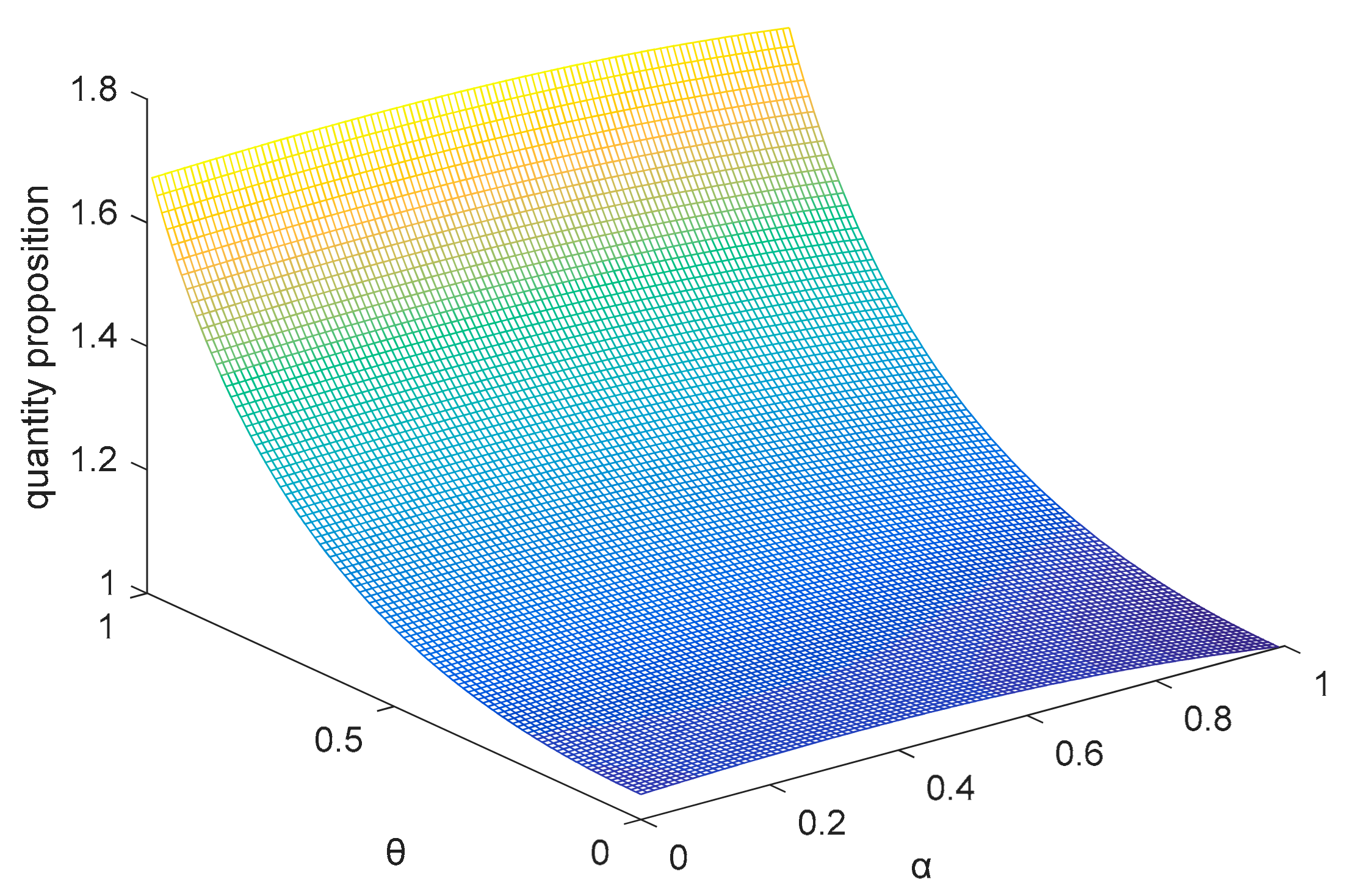
Corollary 2(iv) indicates the optimal proportions of channel quantities only depend on the forward power configuration in Figure 8. The proportion can also be regarded as the channel share. Specifically, the proportion is and only depend on the forward competition intensity if OEM leads the forward channel. However, if the retailer is the leader, the optimal proportion must be less than and might arrive at 1 which is the optimal proportion in the centralized model. Unlike the proportion in the model led by OEM, it decreases in while increases in . Then OEM’s channel share becomes larger.
Now we discuss plausible reasons. If the forward channel led by the retailer, the price battle boosts the total quantities so that OEM’s return rate rises up and his cost reduces. OEM has more incentive to reduce the direct price. In contrast, the retailer’s cost is constant so that his retail price is higher. Then his channel share becomes smaller. If OEM leads the forward channel, faced up with more and more fierce competition, he takes the strategy of offering a higher wholesale price. Even though his direct price is also increasing while the retailer’s cost increases too. This results in the weaker channel competitiveness of the retailer. Then his channel share is also decreasing.
5.3. Dual Competitions
In this section, we first compare different equilibrium profits so that we can analyze CLSC efficiency. In addition, we investigate the extension of M3.
5.3.1. Comparison of Equilibrium Profits
Proposition 6.
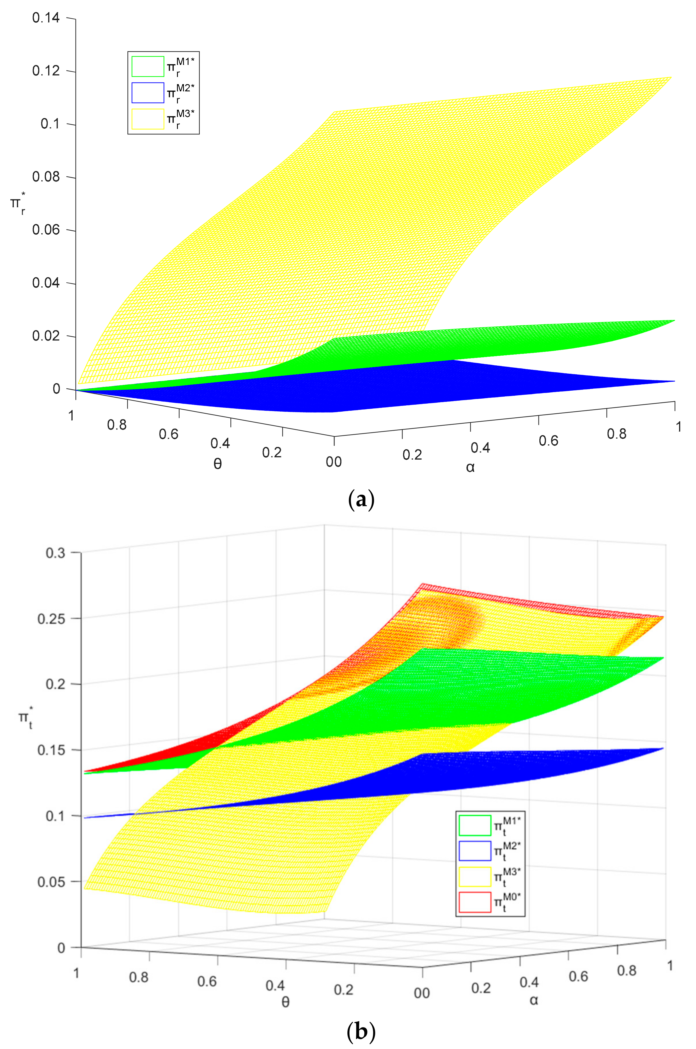
(i) OEM’s, retailer’s and collector’s optimal profits satisfy the following relationships: . If and only if and are larger, . (ii) ; ; (iii) Total channel profits are related as: . With the increase of and , first, , then, .
Intuitively, each channel member obtains the highest profits when they play the leader’s role, respectively. Moreover, from the perspective of CLSC, the profit in the centralized model is the highest. Because all decision variables are fully coordinated and there is no efficiency loss.
From OEM’s perspective, his profit is not the lowest when he holds both second positions in both channels. Even though he leads the forward channel in M2, losing the power of transfer price for him indicates that he might be at an inferior bargaining position to the collector. On the contrary, though his profit from reverse channel and retail channel are both zero, he can still benefit from his direct channel. As goes up, his profit in M2 exceeds that in M3 due to price battle between him and the retailer. Result of battle is that both members’ profits are zero and total quantity attains maximum. Figure 9b shows the impact of and on OEM’s profit. Intuitively, his profit will decrease in , no matter the price war wages in the forward channel. If he leads the forward channel, his profit decreases owing to decreasing sales quantities. Otherwise, his decreasing profit implies that increasing direct quantities cannot offset the loss of decreasing unit profit margin. Moreover, his profit will also decrease in , no matter who leads the reverse channel. Because decreasing reverse return rate results in increasing forward production cost. In summary, both competitions affect OEM’s profit, regardless of its power configuration.
From the retailer’s perspective, the ranking of his profit is aligned with that of his position. Figure 10a shows that his profit declines in competition intensities and eventually tends zero. Likewise, from the collector’s perspective, similar conclusion could be drawn. Clearly, leading whole CLSC is different from leading single reverse channel. The collector has to share the first power with the retailer in M3 so that his profit depends on the negotiation with the retailer. We will discuss the question in next part.
Proposition 6(ii) shows that total profit is the highest in the centralized model owing to no efficiency loss. It is interesting to focus on the following two points. First, when and are smaller, total profit in M3 is so close to that in the centralized model. To optimize the performance of reverse channel, the collector will take the same perspective as does the whole CLSC and his return rate is equal to OEM’s. Meantime, in the forward channel, the retail price is nearly equivalent to the direct price so that the market size is shared equally. Therefore, both channel in M3 is consistent with that in M0. Second, when and are sufficiently high, total profit in M1 is rather close to that in M0. Specifically, if both competition is maximal, i.e., , , total profit in M1 is equal to that in M0. Namely, to hold both first power position for OEM can coordinate CLSC. The implication is that if competitions are fierce, to hold both first positions for OEM is preferred. Otherwise, both opponents will take actions simultaneously so as to maximize their own profits. Namely, from the perspective of CLSC, it is better to concentrate both powers to one OEM. Naturally, when competitions are smaller, it is optimal to hold both second position in both forward and reverse channels for OEM.
5.3.2. Analysis on CLSC Efficiency
Proposition 6(ii) sheds light on CLSC efficiency under dual competitions and power configuration. Then we can obtain Corollary 3.
Corollary 3.
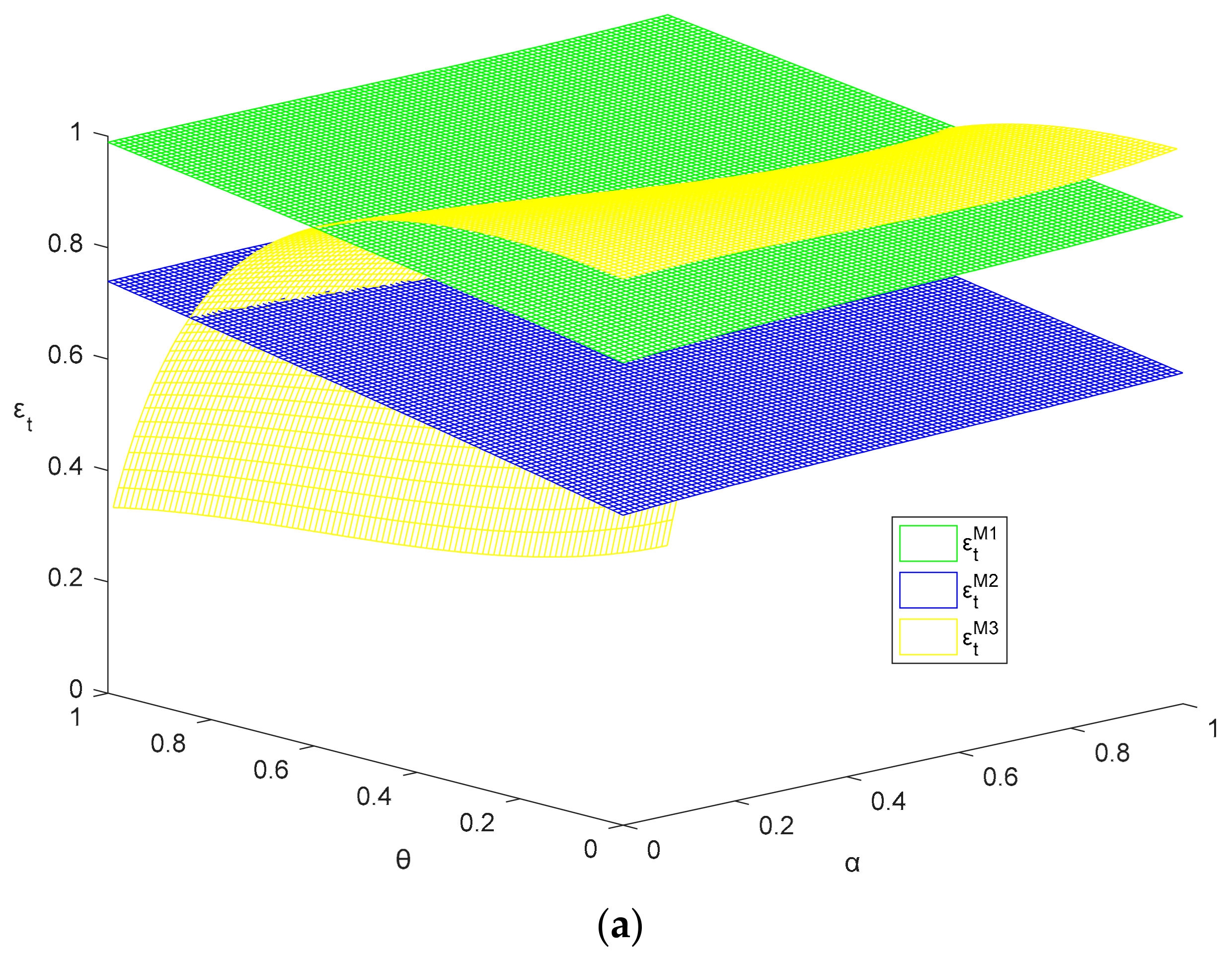
Supply chain efficiency is ordered as: . With the increase of and , first, , then, .
By Corollary 3, we can know the ranking of CLSC efficiency is consistent with that of total profit. It notes the worst CLSC efficiency comes in M2 due to “repeated double marginalization” [7]. Classical double marginalization implies that the wholesale price which is higher than production costs leads to the efficiency loss. If the collector leads the reverse channel in M2, he offers so high transfer price that OEM has to raise the wholesale price. Therefore, “repeated double marginalization” includes two parts, i.e., between collector and OEM in the reverse channel, OEM and retailer in the forward channel.
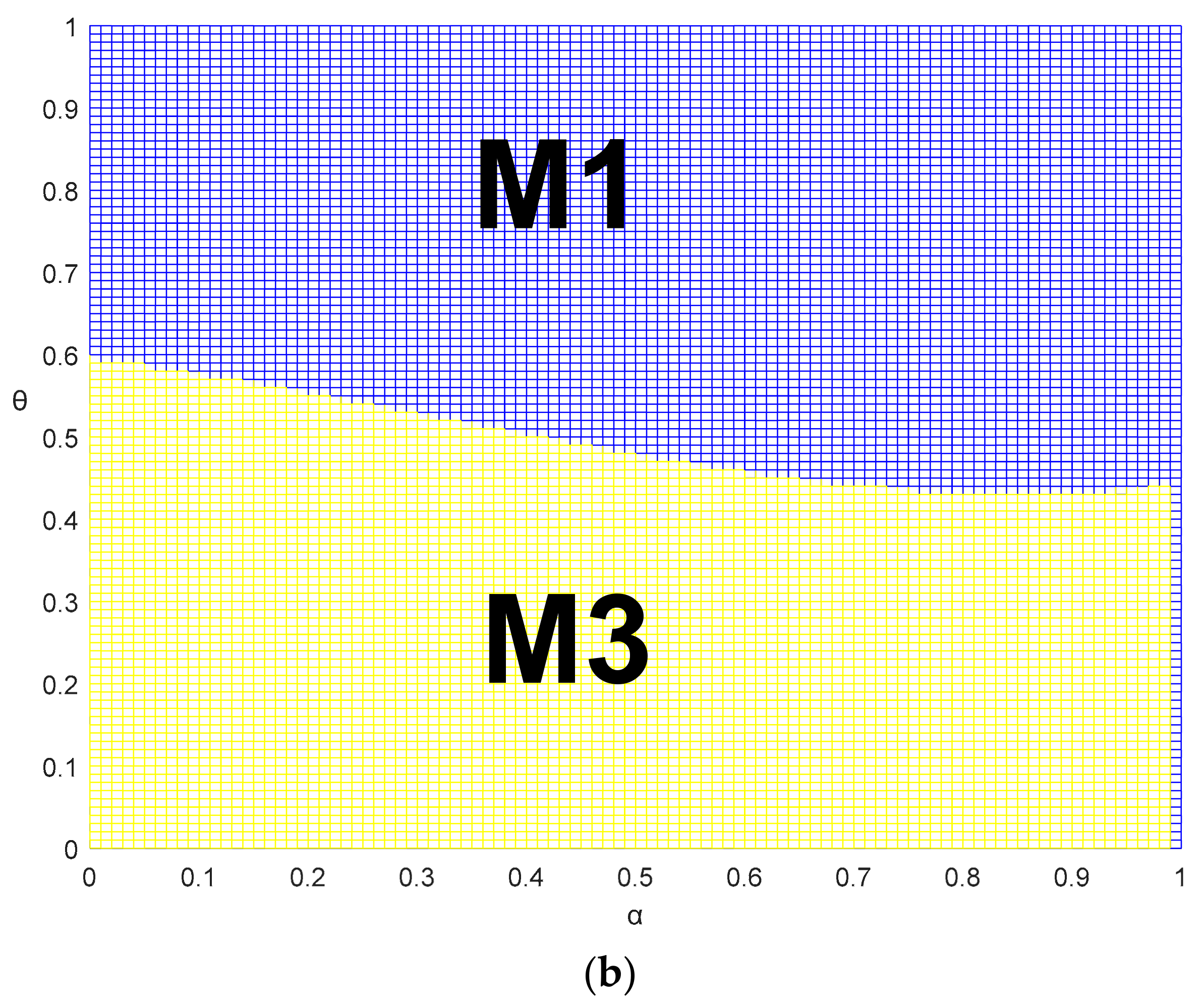
Besides, we analyze the relationship between M1 and M3. In M1, OEM leads both channel while he is follower in both channels in M3. From OEM’s perspective, M1 and M3 are just complementary. By Figure 10b, we can obverse that the performances in both M1 and M3 are far higher than that in M2. Unlike M2, M1 and M3 get rid of “repeated double marginalization” since the condition of the latter is that there is a sequential game between wholesale price and transfer price. But there is either Nash game or no game in M1 and M3. Then M1 and M3 might just suffer from classical double marginalization problem. By Figure 11a, if both competition is maximal, . And if there are nearly no competitions, is close to 1. Figure 11b illustrates there exists a threshold line of and between M1 and M3. Above the threshold line, M1 is preferred; below the line, M3 outperforms. Besides, the observation is that and have the substitution effect since total profit in M0 decreases in both and . Then the threshold line indicates decreases in .
5.3.3. Extension of M3
Unlike OEM who controls both channels in M1, the collector and retailer in M3 lead the reverse and forward competition, respectively. In our analysis for M3, to ensure OEM’s participation, wholesale price is equal to production cost while the transfer price only depends on the reserve competition. Then the collector’s and retailer’s profit just come from single competition so that “repeated double marginalization” disappears. If OEM’s profit is always zero, we can explore the relationship between wholesale price and transfer price. For brevity, we just take unilateral competition into consideration, i.e., , and we can obtain the following theorem.
Theorem 5.
If , , where.
By Theorem 5, we can know wholesale price increases in transfer price. Higher transfer price result in collector’s higher profit, and higher retailer’s profit comes from lower wholesale price. Intuitively, Theorem 5 indicates there is the inverse relationship between the collector’s profit and retailer’s profit. Likewise, Corollary 3 indicates the relationship between wholesale price and transfer price is also positive correlation so that there is “repeated double marginalization” in M2. Different from the case in M2 where the collector is the unique leader, the retailer in M3 also holds the first position. Then it is a key factor for comparison of the retailer’s and collector’s power. If collector has more power, M3 tends to be M2 and “repeated double marginalization” will be more serious so that M3 will be distorted from the full-coordinated channel in M0 more heavily.
6. Conclusions
In this paper, we investigate pricing and collecting decisions in CLSCs under different power configurations and dual competitions. From OEM’s perspective, we build a centralized model and three decentralized models in reflection of OEM’s position in the power configuration. Considering the impacts of both power configuration and dual competition, we provide a systematic comparison of forward competition, reverse competition and dual competitions between four models. The practical implications of the developed models in this study are summarized as follows.
Power configuration plays a significant role in CLSCs for OEM as he competes in both forward and reverse channels. If power configuration determines basic equilibrium level, dual competition intensity shapes the comparative statics of equilibrium. Dual competitions also generate a substitution effect.
First, power configuration indicates who takes control of pricing, which determines how to divide the surplus of the whole system. Reverse pricing, i.e., transfer price determines OEM’s production cost, while forward pricing, i.e., wholesale price could also be regarded as the retailer’s production cost. If double pricing is sequential, “repeated double marginalization” occurs so that pricing and collecting might be distorted twice in model M2. As a consequence, M1 or M3 outperforms. A more powerful collector in M3 will even lead to “repeated double marginalization”. The problem of how CLSC performance is affected by power structure is first examined by Choi et al. [8], who find that the retailer-led model leads to the most effective CLSC. When considering dual competition, however, we reach a different conclusion—that dual leadership (Model M3 in our paper) can benefit the CLSC when the competition is weak.
Second, power configuration determines the channel performance. Return rate could be regarded as reverse channel performance while forward performance depends on sale quantity. Meanwhile, return rate increases in sale quantity so that forward competition influences reverse channel. It is interesting that the division of dual channel profit only depends on the power configuration on their own side, no matter who leads the other side. We note that if reverse channel is led by collector, it will take the same perspective as does the whole CLSC, then his return rate is equal to OEM’s. From the viewpoint of extended producer responsibility (EPR), if reverse competition is not fierce, CPR policy is preferred; otherwise, IPR policy is better.
There is a broad scope to extend the present research. The literature on the closed loop supply chain divides on the assumption whether the price of the new product equals that of the remanufactured. Clearly, we assume in this study there is no distinction between the new and manufactured product. In practice, Kodak single-use camera is a good example of this case, where the firm benefits from the cost reduction, while charging full price for the remanufactured product (Ferrer and Swaminathan [12]). That said, we leave it for future exploration concerning differentiated prices with new and remanufactured products. Another dimension for future research embraces asymmetric information. In particular, the downstream may hold private information on the market demand in the forward channel, while the upstream may hold private information on the market demand in the forward channel, while the upstream may be privately informed of the collection cost in the reverse channel. Either case would call for a formal analysis with asymmetric information. Besides, future research could also consider stochastic demand on end-consumer market.
Author Contributions
Y.Z. defined the proposed problem; Y.L. wrote the paper.
Funding
This work was supported by National Natural Science Foundation of China [grant number 71501108] and Beijing Natural Science Foundation [grant number 9164030].
Conflicts of Interest
The authors declare no conflict of interest.
Appendix A
Proof of Theorem 1.
The Hessian matrix of (3) is
![Sustainability 10 01617 i002]() then , , , , if , , profit function (1) is jointly concave in decision variables.
then , , , , if , , profit function (1) is jointly concave in decision variables.

Then . Taking the first-order partial derivatives of (3) with respect to , we have equilibrium solution. □
Proof of Theorem 2.
It is easy to verify Equation (5) is concave in and (6) is concave in , then the best response of and is given by
Substituting and into Equation (4), we can get,
![Sustainability 10 01617 i003]() where ,. Taking the first-order partial derivatives of with respect to , we can obtain the optimal solutions of . Substituting these optimal solutions into A1, Theorem 2 has been proved. □
where ,. Taking the first-order partial derivatives of with respect to , we can obtain the optimal solutions of . Substituting these optimal solutions into A1, Theorem 2 has been proved. □

Proof of Theorems 3. and 4.
Proofs of Theorems 3 and 4 are similar to the proof of Theorem 2.□
Proof of Proposition 1.
. Clearly, . □
Proof of Proposition 2.
Since , , then . □
Proof of Corollary 1.
We list the return rates, , , , , , then Corollary 1 has been proved. □
Proof of Proposition 3.
It is easy to prove this proposition by Corollary 1. □
Proof of Proposition 4.
Since , and , then wholesale prices are ordered as . □
Proof of Proposition 5.
Since , ,then . As to the comparison between and , we let
Note that decreases in and , , , then there exists thresholds on both and , . If and only if and are smaller, that is to say, , , , i.e., . 5(i) has been proved. The proof of 5(ii) is similar to proof of 5(i). □
Proof of Corollary 2.
Since , , we let , , ,, , , , . Together with Proposition 5 about the ranking of , we can know .The proofs of 2(i) and 2(iii) are similar to above proof. Since , , , meantime, . Also, we can know . □
Proof of Proposition 6.
First, we compare the retailer’s profit. According to Corollary 2, we also let , . , then . Besides, . Clearly, , then the retailer’s profits are ordered as .
Second, we compare the collector’s profit. , , . Combined with , we can know .
Third, we compare OEM’s profits. Sincethen we compare with . Easy to know , we let . decreases in and , , , then there exists thresholds on both and , . If and only if , , , i.e., .
As to the comparison of total CLSC’s profits, easy to know , , then . In a similar way to compare with , we can make the comparison between , and . □
Proof of Corollary 3.
Since and , it is easy to obtain . Note that decreases in both and . If , is the largest and , , . If , is the smallest and , .
Proof of Theorem 5.
If , , , , then we can get . Rearranging the equation, Theorem 5 has been proved. □
References
- Wu, C.H. Price and service competition between new and remanufactured products in a two-echelon supply chain. Int. J. Prod. Econ. 2012, 140, 496–507. [Google Scholar] [CrossRef]
- Electronics TakeBack Coalition. Brief Comparison of State Laws on Electronics Recycling. 2013. Available online: http://www.electronicstakeback.com/wp-content/uploads/Compare_state_laws_chart.pdf (accessed on 16 May 2018).
- Subramanian, R.; Gupta, S.; Talbot, B. Product design and supply chain coordination under extended producer responsibility. Prod. Oper. Manag. 2009, 18, 259–277. [Google Scholar] [CrossRef]
- Atasu, A.; Subramanian, R. Extended producer responsibility for e-waste: Individual or collective producer responsibility? Prod. Oper. Manag. 2012, 21, 1042–1059. [Google Scholar] [CrossRef]
- Bulmus, S.C.; Zhu, S.X.; Teunter, R. Competition for cores in remanufacturing. Eur. J. Oper. Res. 2014, 233, 105–113. [Google Scholar] [CrossRef]
- Bulmus, S.C.; Zhu, S.X.; Teunter, R. Optimal core acquisition and pricing strategies for hybrid manufacturing and remanufacturing systems. Int. J. Prod. Res. 2014, 52, 6627–6641. [Google Scholar] [CrossRef]
- Huang, M.; Song, M.; Lee, L.H.; Ching, W.K. Analysis for strategy of closed-loop supply chain with dual recycling channel. Int. J. Prod. Econ. 2013, 144, 510–520. [Google Scholar] [CrossRef]
- Choi, T.M.; Li, Y.J.; Xu, L. Channel leadership, performance and coordination in closed loop supply chains. Int. J. Prod. Econ. 2013, 146, 371–380. [Google Scholar] [CrossRef]
- Chiang, W.Y.K.; Chhajed, D.; Hess, J.D. Direct marketing, indirect profits: A strategic analysis of dual-channel supply-chain design. Manag. Sci. 2003, 49, 1–20. [Google Scholar] [CrossRef]
- Mukhopadhyay, S.K.; Zhu, X.; Yue, X. Optimal contract design for mixed channels under information asymmetry. Prod. Oper. Manag. 2008, 17, 641–650. [Google Scholar] [CrossRef]
- Zheng, B.; Yang, C.; Yang, J.; Zhang, M. Dual-channel closed loop supply chains: Forward channel competition, power structures and coordination. Int. J. Prod. Res. 2017, 55, 3510–3527. [Google Scholar] [CrossRef]
- Turki, S.; Didukh, S.; Sauvey, C.; Rezg, N. Optimization and analysis of a manufacturing–remanufacturing–transport–warehousing system within a closed-loop supply chain. Sustainability 2017, 9, 561. [Google Scholar] [CrossRef]
- Huang, Y.; Wang, Z. Dual-Recycling Channel Decision in a Closed-Loop Supply Chain with Cost Disruptions. Sustainability 2017, 9, 2004. [Google Scholar] [CrossRef]
- Son, D.; Kim, S.; Park, H.; Jeong, B. Closed-Loop Supply Chain Planning Model of Rare Metals. Sustainability 2018, 10, 1061. [Google Scholar] [CrossRef]
- Ferrer, G.; Swaminathan, J.M. Managing new and remanufactured products. Manag. Sci. 2006, 52, 15–26. [Google Scholar] [CrossRef] [Green Version]
- Ferrer, G.; Swaminathan, J.M. Managing new and differentiated remanufactured products. Eur. J. Oper. Res. 2010, 203, 370–379. [Google Scholar] [CrossRef] [Green Version]
- Ferguson, M.E.; Toktay, L.B. The effect of competition on recovery strategies. Prod. Oper. Manag. 2006, 15, 351–368. [Google Scholar] [CrossRef]
- Webster, S.; Mitra, S. Competitive strategy in remanufacturing and the impact of take-back laws. J. Oper. Manag. 2007, 25, 1123–1140. [Google Scholar] [CrossRef]
- Balasubramanian, S. Mail versus mall: A strategic analysis of competition between direct marketers and conventional retailers. Market Sci. 1998, 17, 181–195. [Google Scholar] [CrossRef]
- Cattani, K.D.; Gilland, W.G.; Swaminathan, J.M. Coordinating traditional and internet supply chains. In Handbook of Quantitative Supply Chain Analysis: Modeling in the E-Business Era; Simchi-Levi, D., Ed.; Kluwer: Boston, MA, USA, 2004; pp. 643–677. [Google Scholar]
- Cattani, K.; Gilland, W.; Heese, H.S.; Swaminathan, J. Boiling frogs: Pricing strategies for a manufacturer adding a direct channel that competes with the traditional channel. Prod. Oper. Manag. 2006, 15, 40–56. [Google Scholar]
- Savaskan, R.C.; Bhattacharya, S.; Van Wassenhove, L.N. Closed-loop supply chain models with product remanufacturing. Manag. Sci. 2004, 50, 239–252. [Google Scholar] [CrossRef]
- Nie, J.; Huang, Z.; Zhao, Y.; Shi, Y. Collective recycling responsibility in closed-loop fashion supply chains with a third party: Financial sharing or physical sharing? Math. Probl. Eng. 2013, 2013, 301–312. [Google Scholar] [CrossRef]
- Shi, Y.; Nie, J.; Qu, T.; Chu, L.K.; Sculli, D. Choosing reverse channels under collection responsibility sharing in a closed-loop supply chain with re-manufacturing. J. Intell. Manuf. 2015, 26, 387–402. [Google Scholar] [CrossRef]
- Gui, L.; Atasu, A.; Ergun, O.; Toktay, L.B. Design incentives under collective extended producer responsibility: A network perspective. Manag. Sci. 2018. [Google Scholar] [CrossRef]
- Hong, X.; Wang, Z.; Wang, D.; Zhang, H. Decision models of closed-loop supply chain with remanufacturing under hybrid dual-channel collection. Int. J. Adv. Manuf. Technol. 2013, 68, 1851–1865. [Google Scholar] [CrossRef]
- Karakayali, I.; Emir-Farinas, H.; Akcal, E. An analysis of decentralized collection and processing of end-of-life products. J. Oper. Manag. 2007, 25, 1161–1183. [Google Scholar] [CrossRef]
- Maiti, T.; Giri, B.C. A closed loop supply chain under retail price and product quality dependent demand. J. Manuf. Syst. 2015, 37, 624–637. [Google Scholar] [CrossRef]
- Gao, J.; Han, H.; Hou, L.; Wang, H. Pricing and effort decisions in a closed-loop supply chain under different channel power structures. J. Clean. Prod. 2016, 112, 2043–2057. [Google Scholar] [CrossRef]
- Ingene, C.A.; Parry, M.E. Bilateral monopoly, identical distributors, and game-theoretic analyses of distribution channels. J. Acad. Market. Sci. 2007, 35, 586–602. [Google Scholar] [CrossRef]
- Yan, Y.; Zhao, R.; Chen, H. Prisoner’s dilemma on competing retailer’s investment in green supply chain management. J. Clean. Prod. 2018. [Google Scholar] [CrossRef]
Figure 1.
Dual-competition closed loop supply chains (CLSCs).

Figure 2.
The impact of and on the optimal transfer price. (a); (b) .

Figure 3.
The impact of and on the optimal return rate. (a) ; (b) .

Figure 4.
The impact of and on the optimal wholesale price. (a) ; (b) .

Figure 5.
The impact of and on the optimal retail price and direct price. (a) ; (b) .

Figure 6.
The impact of and on the optimal direct and retail quantities. (a) ; (b) .

Figure 7.
The impact of and on the optimal total quantities.

Figure 8.
The impact of and on the optimal quantity proportion.

Figure 9.
The impact of and on equilibrium profits. (a) ; (b) .
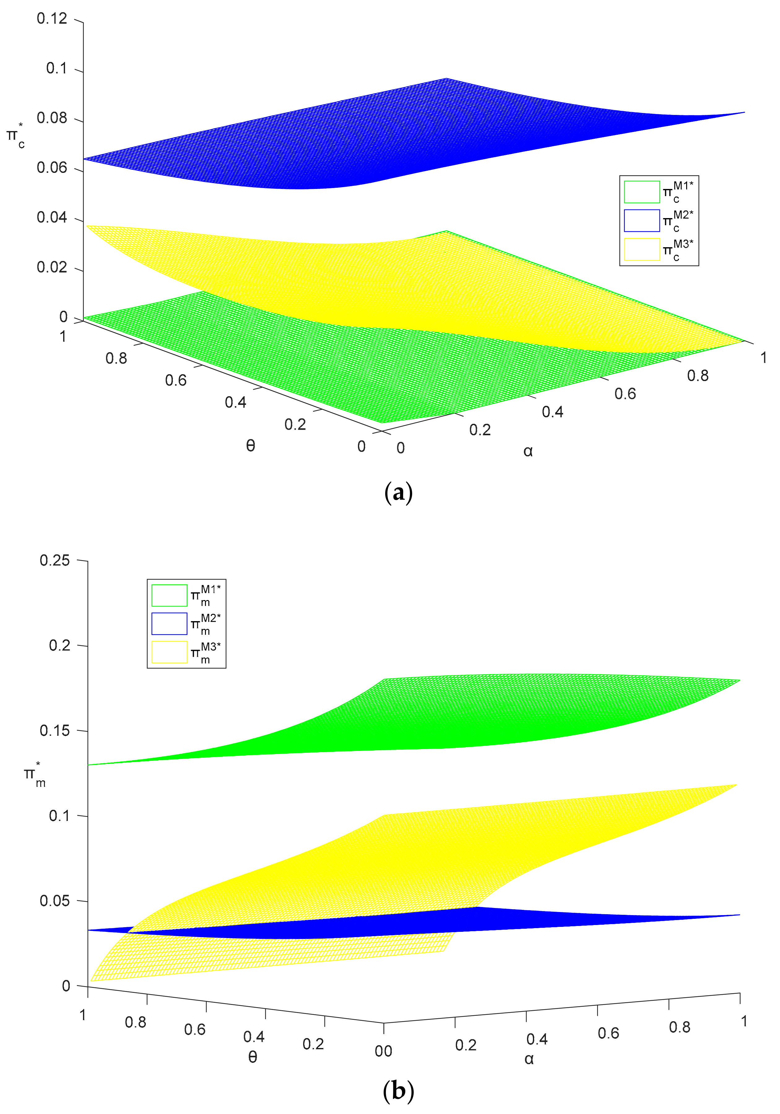
Figure 10.
The impact of and on equilibrium profits. (a) ; (b) .

Figure 11.
The impact of and on CLSC efficiency. (a) ; (b) comparison between and .

Table 1.
Description of Related Symbols.
| Symbol | Description |
|---|---|
| Decision variables | |
| Direct/retail price in model j | |
| Return rate of OEM/collector in model j | |
| Wholesale price in model j | |
| Transfer price in model j | |
| Parameter | |
| Unit cost of producing a new/remanufactured product | |
| Saving unit cost by remanufacturing, | |
| C | The exchange coefficient between the return rate and investment on recycling |
| Reverse/forward competition intensity between reverse/forward members | |
| Investment of collector/OEM in collection process | |
| Sales quantities of direct/retail/total channel in model j | |
| Total return rate in model j | |
| Profit of channel member i in model j | |
| Supply chain efficiency in model j, | |
Subscript refers to OEM (m), retailer (r), collector (c) and total CLSC (t), respectively. Superscript represents to Model M0, M1, M2, M3, respectively. The asterisk (*) is imposed to denote the optimal value of the variable concerned.
© 2018 by the authors. Licensee MDPI, Basel, Switzerland. This article is an open access article distributed under the terms and conditions of the Creative Commons Attribution (CC BY) license (http://creativecommons.org/licenses/by/4.0/).
Share and Cite
MDPI and ACS Style
Liu, Y.; Zhang, Y. Closed Loop Supply Chain under Power Configurations and Dual Competitions. Sustainability 2018, 10, 1617. https://0-doi-org.brum.beds.ac.uk/10.3390/su10051617
AMA Style
Liu Y, Zhang Y. Closed Loop Supply Chain under Power Configurations and Dual Competitions. Sustainability. 2018; 10(5):1617. https://0-doi-org.brum.beds.ac.uk/10.3390/su10051617
Chicago/Turabian StyleLiu, Yang, and Yang Zhang. 2018. "Closed Loop Supply Chain under Power Configurations and Dual Competitions" Sustainability 10, no. 5: 1617. https://0-doi-org.brum.beds.ac.uk/10.3390/su10051617
Note that from the first issue of 2016, this journal uses article numbers instead of page numbers. See further details here.