Article

Parametric Optimization of Window-to-Wall Ratio for Passive Buildings Adopting A Scripting Methodology to Dynamic-Energy Simulation

1
Department of Architecture and Design, Politecnico di Torino, Turin 10125, Italy
2
Department DIST, Politecnico di Torino, Turin 10125, Italy
3
Department DAUIN, Politecnico di Torino, Turin 10138, Italy
4
ICT for Smart Societies, Department DET, Politecnico di Torino, Turin 10138, Italy
*
Author to whom correspondence should be addressed.
Sustainability 2019, 11(11), 3078; https://0-doi-org.brum.beds.ac.uk/10.3390/su11113078
Submission received: 16 May 2019 / Revised: 26 May 2019 / Accepted: 28 May 2019 / Published: 31 May 2019

Abstract

:
Counterbalancing climate change is one of the biggest challenges for engineers around the world. One of the areas in which optimization techniques can be used to reduce energy needs, and with that the pollution derived from its production, is building design. With this study of a generic office located both in a northern country and in a temperate/Mediterranean site, we want to introduce a coding approach to dynamic energy simulation, able to suggest, from the early-design phases when the main building forms are defined, optimal configurations considering the energy needs for heating, cooling and lighting. Generally, early-design considerations of energy need reduction focus on the winter season only, in line with the current regulations; nevertheless a more holistic approach is needed to include other high consumption voices, e.g., for space cooling and lighting. The main considered design parameter is the WWR (window-to-wall ratio), even if further variables are considered in a set of parallel analyses (level of insulation, orientation, activation of low-cooling strategies including shading devices and ventilative cooling). Finally, the effect of different levels of occupancy was included in the analysis to regress results and compare the WWR with corresponding heating and cooling needs. This approach is adapted to Passivhaus design optimization, working on energy need minimisation acting on envelope design choices. The results demonstrate that it is essential to include, from the early-design configurations, a larger set of variables in order to optimize the expected energy needs on the basis of different aspects (cooling, heating, lighting, design choices). Coding is performed using Python scripting, while dynamic energy simulations are based on EnergyPlus.

1. Introduction

Buildings are responsible for more than 40% of the total primary energy consumption in industrialized countries [1,2,3,4], and roughly one third of the relevant GHG emissions. Considering this great influence of the building sector on national energy balances, several actions have been taken by government institutions in order to: firstly, reduce the building energy needs; secondly, increase the efficiency of the installed equipment; and thirdly, increase the amount of energy produced by renewable sources. At the European level, the EPBD directive and further upgrading—see the EPBD recast and the recent Directive 2018/844—have progressively acted on the reduction of energy needs and consumptions, while other directives, such as the 2009/28/EC, have worked to promote the usage of renewable sources. Nevertheless, while much attention was paid to reducing heating energy consumption, the reduction of cooling energy needs has not elicited the same consideration. Cooling energy needs have been constantly growing due to several causes, including climate change, international building styles, and changes in the culture of comfort [5,6,7]. Furthermore, the adoption of extended insulation levels may cause an increase in overheating effects—see for example [8,9]. The need to include in the design process low-energy cooling strategies in order to correctly balance energy needs was also underlined by several authors [10,11].

1.1. WWR and energy needs – a short background analysis

Design optimization studies, considering both winter and summer effects, are essential to avoid the adoption of flawed design decisions from the sustainable/environmental point of view. The impact of envelope design choices on energy needs is evident. Among several design aspects related to envelope definition, the ratio of transparent and opaque areas, i.e. the WWR (Window-to-Wall Ratio), is recognized to have a high impact on building energy balances [12]. Since the 1970s, studies have been conducted to define optimal WWR values corresponding to the minimal annual energy needs [13,14]. Nevertheless, these first analyses do not include the effect of passive cooling solutions (e.g., shading systems or CNV) nor the impact of internal gain (occupancy) variations. The relationship between WWR and energy needs was also studied in the 1990s within the EC-funded Project LT (lighting thermal), wherein the influence of WWR on lighting, space cooling and heating in buildings, for average southern European climate conditions, was analysed. Results showed that the minimum yearly-balanced energy consumption in a residential building could be found at WWR values of: 8%, 10%, 15%, respectively for horizontal, East/West, and South/North window exposure, if windows are not shaded; 10%, 15%, 20%, and 30%, respectively, for horizontal, North, East/West, and South window exposure, with 65% of windows shaded [15]. However, this analysis was based on a simplified calculation method and did not include the effect of occupancy nor the impact of passive cooling solutions (e.g., CNV), nor the effect of different levels of insulation.
In 2010, the relation between WWR and thermal energy needs, was studied for a large office building in Shanghai, China, including life cycle assessment results. Nevertheless, only thermal results were included based on a spreadsheet calculation. In total, 63 cases were simulated showing a positive correlation between an increase in the WWR and an environmental impact reduction [16]. Also, in this case, passive cooling solutions and internal gains were not considered, while the effect of WWR on lighting was also not investigated. Another approach was presented in [17], focusing on the effect that climate indicators, i.e. the ambient temperature amplitude, and envelope U-value have on the definition of the maximum WWR for reaching thermal autonomy in buildings. 135 simulations were carried out considering seven U.S. locations. For this analysis no HVAC systems were included considering free-running operation. Results underline the need to define methodologies able to suggest WWR values from the early-design approaches to consider local climates and different envelope thermal transmittances. Authors further suggest the usage of statistical correlations in further studies. No passive cooling solutions, nor internal gains or lighting needs are considered in this analysis.
Furthermore, geographical studies on optimal WWR definition were conducted in Ref. [18], considering five Asian locations, and in Ref. [19], focusing on four locations, two in U.S. and 2 in Europe. The first study investigated the relation between WWR and total energy performance, while the second focused on energy needs for heating and cooling. In both cases no passive cooling solutions or internal gain variations were assumed. Differently, a detailed analysis on optimal WWR definition in relation to energy needs for heating, cooling and lighting was performed for four European locations [20]. This paper includes the effect of shading systems by also considering different activation flux thresholds. A low energy office building was simulated in EnergyPlus considering one U-value configuration. Internal loads were defined in compliance to standard values. A sensitivity analysis was also conducted considering building compactness, equipment efficiency and artificial light efficiency. In addition, natural light analyses were performed considering the UDI and the DA indexes. The investigation is based on five WWR in order to define potential correlation curves. Nevertheless, this study does not include CNV, random internal gain variations, or the impact of different U-value on results.
Other recent studies [21,22] have also defined potential optimization levels for WWR. Interesting graphical models for designers were produced referring to a middle European case study of a sample shaped building simulated in EnergyPlus with average levels of insulation and no internal gains. These graphs include cooling and heating energy needs for different orientations in the range E-S-W, different building shapes and three WWR values [21]. Furthermore, an optimisation analysis to define some envelope characteristics for a sample building within rural and urban contexts was also produced in [22] considering dynamic energy simulations including heating, cooling and lighting energy needs. In particular, this study refers to the number, dimension, position of windows and wall thickness. A parametric investigation of Italian conditions was carried out in 2017 [23] considering 12 locations, different U-values, i.e., low and high insulation, and for the latter, normal and spectral selective glazing cases, and seven WWR steps for a total of 518 simulations. In this analysis, the shading effect was also included considering electrochromic glazing, but not the effect of CNV or internal gain variations. The authors underlined the high effect of climate on optimal WWR, while other aspects did not seem to vary considerably this parameter, even if they suggested to analyse them more in details. In the same year in Ref. [24], the relation between WWR and window orientation for an office building localize in Tripoli, Libya, was investigated. The considered case study is simplified by a schematic box with one non adiabatic wall confining with the external environment. Eight orientations and 10 WWR steps were considered for this analysis conducted via EnergyPlus. The analysis focuses on cooling and heating loads, while other aspects are fixed in accordance to ASHRAE suggestions. Results showed a direct correlation between annual energy needs (cooling and heating) and WWR in all orientations, even if this effect was higher for southern cases (SE, S, SW, W). This study did not include the effect of natural light balance, passive cooling solutions (nor shading or CNV), nor internal gain variations or the influence of different U-values or climates, even if some of these aspects are expected to be included in future developments.
A method to map the suggested WWRs was investigated in [25] for 10 Japan locations. Three classes were defined: (i) WWR directly related to CO2 emission, (ii) optimal WWR minimizing CO2 can be defined, (iii) WWR and CO2 are inversely correlated. A typical office building was used as reference case study to perform EnergyPlus dynamic energy simulations. Results included cooling, heating and lighting energy needs, considering they transposition in equivalent CO2 emissions [kg]. Four orientations, two lighting powers (5 and 10 W/m2), and seven WWRs were included in the proposed approach. Fixed thermal properties were assumed by national standards. This paper also investigated the effect of three internal gain levels by varying together occupancy and equipment densities. Results showed that internal gains principally effected CO2 emissions levels, even if, in some cases, they also influence the optimal WWR. Results suggested that this aspect may be further investigated. Nevertheless, the effect of passive cooling strategies or different thermal envelope characteristics were not included. Furthermore, the correlation between NZEB buildings and WWR was investigated in [26], considering a severely cold China location (Shenyang). A simple building was simulated in EnergyPlus to define heating and cooling energy needs in accordance with different WWRs and three orientations. Considering the rigid climate condition, a direct relation between the WWR and the energy needs was underlined for all orientations. Fixed thermal characteristics of the building were adopted. No passive cooling solutions, U-value, internal gain variations, daylight balance, or regression analyses were considered.
In 2019 the correlation between energy and daylight performance of a sample office room south-oriented for different WWRs was tested considering different percentage of integration of CdTe PV gazing in windows [27]. Five locations, representative of each Chinese climate zone, were selected. A total of 28 cases were simulated for each of them, considering 4 WWR steps and different PV integration percentages. Results showed that PV windows can help in reducing energy needs in office buildings starting from large WWR, ≥45%. This study is based on EnergyPlus and Radiance. No thermal characteristics or internal gain variations are considered. Furthermore, the effect of passive cooling solutions was not investigated. Finally, an optimization analysis of WWR in China low latitude region were presented in 2019 [28] considering also the effect of fixed external sunshade systems (overhang, vertical and comprehensive cases). Cooling, heating and lighting energy needs were considered in this optimization analysis. A sample hotel building was assumed as a reference to perform the simulations in EnergyPlus and Radiance considering four orientations. Results from both software programs were used to optimize the WWR. These analyses aimed to correlate the minimal WWR to reach daylight standards with energy consumptions.
The present paper focuses on the influence that specific façade design choices have on the expected building energy needs for heating, cooling and lighting in the preliminary phase, when the possibility to change is higher and its cost lower, assuming an environmental and technological approach—see [29]. This approach is consistent with the “passive house” concept as developed by the Passive House Institute of Darmstad, Germany [30]. In particular, the presented analysis deals with the influence of WWR on the energy need of an office building, in combination to other parameters such as envelope Uvalue [31], windows orientation, shading coefficient, and controlled natural ventilation (CNV) to perform ventilative cooling, i.e., wind-driven and stack-driven airflow through openings controlled by motorised actuators linked to microclimate sensors. The dynamic energy simulations were carried out using EnergyPlus and Python for two reference locations. The proposed investigation not only analyses the obtained results considering the proposed case studies, but is based on the elaboration of a code that can be used to model the optimal WWR in different locations or for different configurations. Furthermore, the reliability of results was checked under the influence of random internal gain variations (occupancy level) in order to define the statistical correlation curves. The adoption of a scripting simulation approach allows, in fact, to increase the number of performed simulations by two or three orders of magnitude with respect to previous analyses. Thanks to the inclusion of all these aspects, the followed approach can be considered innovative in comparison to previous research on the topic.

1.2. The Research Objective and Structure

The main objective of this study was to develop an algorithm to optimise, from the early-design phase, the WWR of an office building for reducing the expected energy needs for space heating and cooling, and lighting to the levels required by the Passive House concept. This study was conducted following a multidisciplinary approach, based on the collaboration between ICT Master Degree students and researchers from different fields: architectural technology and environmental design, telecommunication engineering, and data elaboration. The proposed approach is suited to the design of new constructions as well as major building refurbishments, and it is applied here to two locations: one, Helsinki, with a harsh winter climate; the other, Turin, with a temperate climate, located in the enlarged Mediterranean area. Of course, the methodology of this paper can be applied to different climates in order to demonstrate how design optimisation choices differs according to environmental conditions.
In addition to WWR, other parameters were considered in the energy optimisation analysis: envelope thermal transmission (opaque and transparent); CNV; and window shading coefficient. Two different European locations, Helsinki and Turin, representing, respectively, cold and temperate climate conditions, were considered. Moreover, the effect of random changes in the occupancy level was included in the analysis to improve the resilience of the proposed optimisation models in relation to the impact of internal gains variations (i.e., the presence of people).
The paper is structured as follows: in Section 2 the proposed methodology is introduced; Section 3 describes the results of the WWR optimisation process; Section 4 is related to the discussion of results including the effect of random occupancy and monthly evaluation of heating, cooling and lighting energy needs; paper’s conclusions are described in Section 5.

2. Materials and Methods

The proposed approach is based on the definition of a script to generate parametric analysis outputs, e.g., graphs, showing the energy needs for the heating, cooling and lighting of a sample office unit as function of WWR. The simulation programmes used are: Design Builder v5.5 (DB) (DesignBuilder Software Ltd, Gloucs, UK), to generate the starting case study; EnergyPlus, to perform dynamic energy simulations; and Python, to control the whole process, modify input data, collect simulation results, and analyse output data including graph elaborations.
DB was used to create the 3D model of the reference office-building unit, described in Section 2.1., while EnergyPlus was used—via a Python script—to simulate its energy needs for various envelope configurations, and for generating the relevant *.idf files. The Python library Geomeppy, allowed for changing parametrically WWR as well as running directly simulations, without using the EnergyPlus interface each time, was adopted.
Furthermore, a sensitivity analysis, able to consider the potential variation effect in energy needs due to random variations in the internal loads, was carried out. These variations were based on the occupancy levels, simulating real operation, without adding equipment, which will be the topic of a future improvement of the method. In each simulation, the standard occupancy datum defined in DB —standard office schedule—was let varying randomly according to a Gaussian distribution—G(μ,σ), with μ = 0.09225 people/m2 and σ = 0.14075 people/m2—in order to make a more realistic impact on the energy needs of the internal-gain variations due to the presence of people. The variation domain was adapted by [32]. A sample plot of 10,000 random values extracted by the adopted Gaussian is reported in Figure 1 in order to show, considering the central limit theorem, that the chosen values are statistically reasonable. The values reported in this figure refer to the net simulated office area of 80 m2.
Simulation outputs include heating and cooling, as well as annual lighting energy needs. The light requirement was set to 400 lux at desk height, balancing illuminance requirements on task and surrounding areas for offices according to UNI EN 12464-1 while the linear dimmer control was assumed in EnergyPlus to balance the positive effect of natural lighting with the additional need for artificial sources. Internal normalised light loads were assumed to be 5 W/m2-100lux. This value is of course balanced by the software in accordance to the amount of natural light calculated by EnergyPlus. The use of this dynamic simulation tool to also simulate natural/artificial balance was demonstrated to be effective by several authors, see for example the discussion in [20]. Heating and cooling set points were assumed to be respectively 20 °C and 26 °C.
The analysis was carried out according to the following phases.
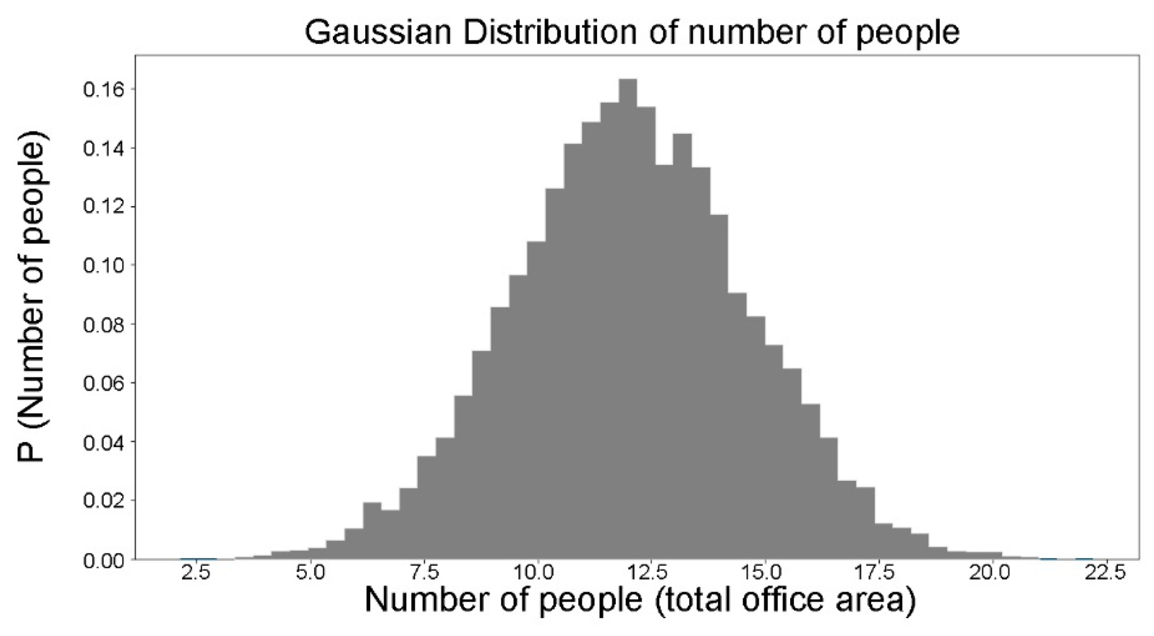
  • A simulation with occupancy level constant during the year and varying WWR from 1% to 95%, by a step of 5%.
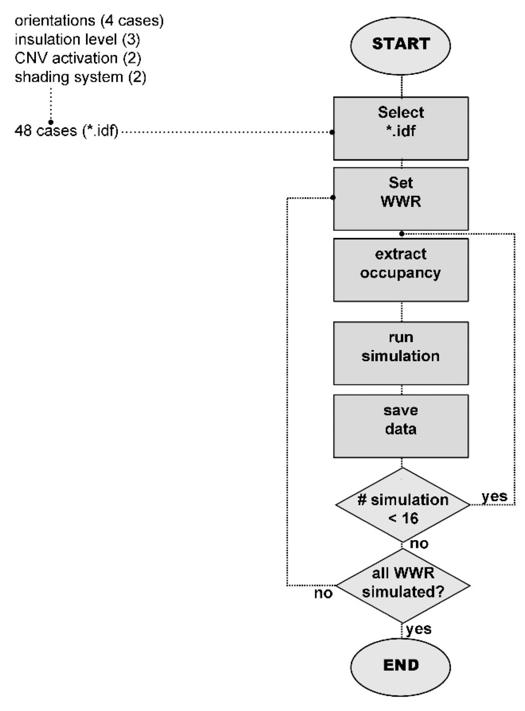
  • Simulations with variation of the occupancy level within a 16-values range for each configuration, based on the above-mentioned Gaussian distribution; and 16128 runs for each location, considering the 21 WWR variations and the 48 building configurations described in Section 2.1. This step aimed at creating train and test datasets for statistical analyses.
  • Regression analyses of the output data, divided in train—to develop the regression—and test sets by a ratio 70–30%, as well as a calculation of the RMSE of the regression with respect to the independent test database.
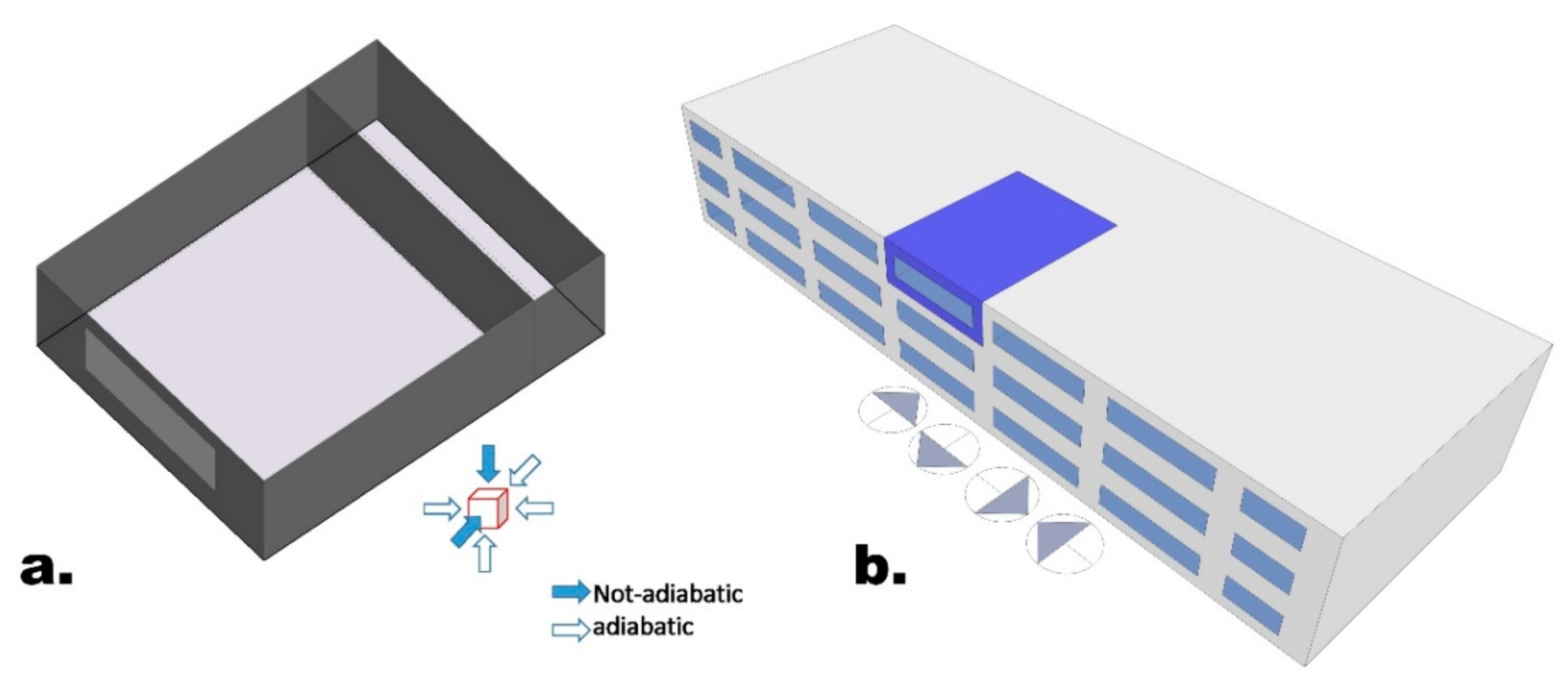
Figure 2 shows a flowchart of the developed simulation engine.

2.1. The Case Study

The case study is an office space unit virtually included in a multi-storey building as shown in Figure 3. The walls adjacent to the other space units and the floor are assumed as adiabatic, while one wall and the roof are external surfaces. The net area of the space unit was set to 80 m2 considering an open office space, while the infiltration rate was fixed to 0.7 ACH
The configurations applied in simulation are the following:
-
Two locations, i.e., Helsinki (FIN) and Turin (ITA);
-
Three values of the envelope heat transmission coefficient (Uvalue) corresponding to low, medium, and high insulation levels (see Table 1 for the opaque envelope, and Table 2 for windows);
-
Four orientations of the external wall, i.e., South, East, West, and North;
-
Shading devices set according to the integrated shading control system of DB—see below—(present/not present) and;
-
CNV set to on and off.
Without considering locations, 48 configurations were assumed.
Figure 4 shows materials and layers of the opaque envelope (external wall and roof) in the three considered configurations.
The external wall has one window whose dimensions were changed automatically acting on the WWR indicator. In addition, the effects of shading and CNV were considered, together or singularly. In particular, for shading devices an integrated external located blind system with medium reflectivity slats was assumed. The control type for this shading considers both an external air temperature threshold and a solar radiation set point. The first was set to 18 °C, considering the effect of office equipment [33] in comparison to the potential threshold for residential buildings of 21 °C suggested by Olgyay [34], while the second was assumed as 120 W/m2, in line with the suggested set points—e.g., [33]. Differently, CNV was simulated considering summer activation with a maximal external air control set to 26 °C and a fixed ACH of 6 vol/h in line with ACH values used in other references for early-design [8]. CNV is principally conceived to be naturally-driven, even if small fan-assisted extractors may be activated when buoyancy or wind-driven flows are not sufficient for cooling purposes. In accordance with other ventilative cooling approaches for early-design stages—e.g., early analysis of CNV climate potential by IEA EBC Annex 62—CNV evaluations were performed without including fan energy consumption assuming the prevalent natural-driven force. This is in accordance with the definition of the specific list of input parameters for programmed natural ventilation in EnergyPlus (early-design option). Section 3 describes the simulation results for the 48 combinations assumed for each location.

3. Simulation Results and Analysis

The first analysis step was performed by running all the simulations considering a constant occupancy schedule while changing the WWR. Here, “constant occupancy” means that the only variation of the occupancy happens through the schedule of Design Builder and the mean occupancy value remains constant throughout the year. The schedule used for simulating the occupancy during the day is suited for an open plan office area as provided by the file OpenOff_Occ of DesignBuilder [35].
Figure 5 shows the results of simulations for all configurations and setups, including shading and CNV settings, for the Helsinki case, while Table 3 reports the optimal WWR [%] and related total energy needs [kWh/m2]. At a first glance, the minimum energy need corresponds to 95% WWR in the high insulated scenario for the South window orientation when both CNV and shading are activated. This is due to the high energy contribution of solar gains in winter, with an optimal control of the potential overheating in summer, as allowed by the South window exposure at the considered high Northern latitude [36,37]. Differently, with the North-facing window the minimum energy need is reached at 55% of WWR with shading system set to off due to the prevailing need for reducing heat losses in winter. East and West window orientations show similar behaviour.
In addition, the higher the WWR, the lower the energy needs for lighting. The above-mentioned behaviours are even more apparent in the cases of “non-insulated” and “medium-insulated” scenarios.
Similarly, Figure 6 shows the final simulation results on the annual energy needs for heating, cooling, and lighting of the reference office-building unit located in Turin in all envelope configurations, while Table 4 reports optimal WWR and total energy needs for all considered cases. The following comments could be made on these results
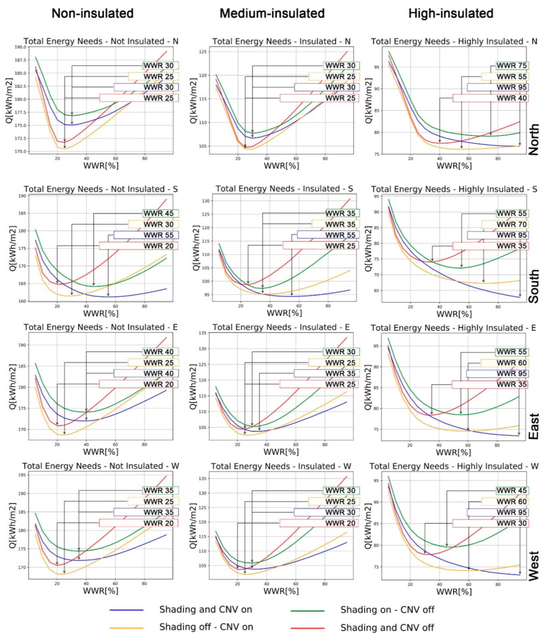
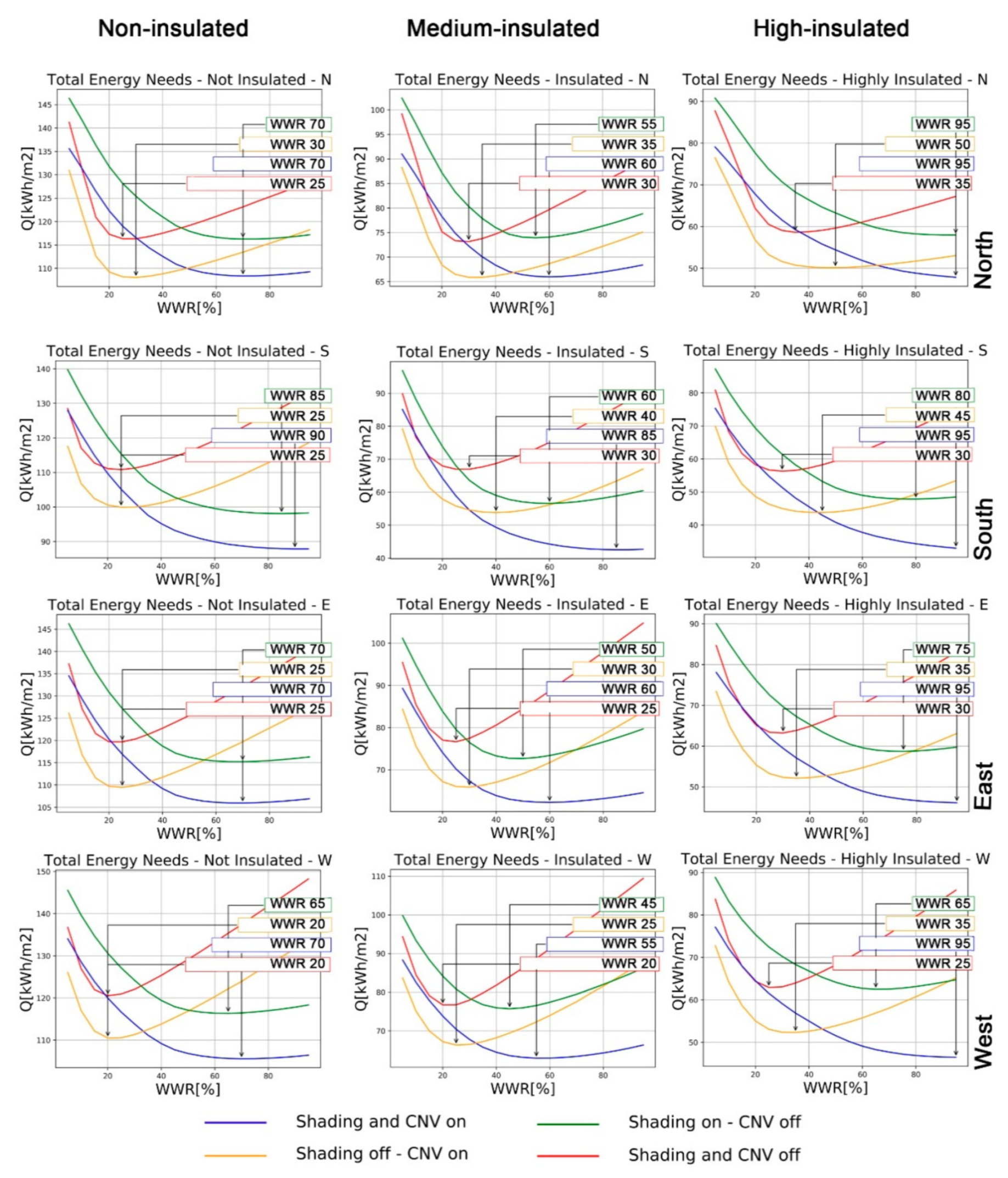
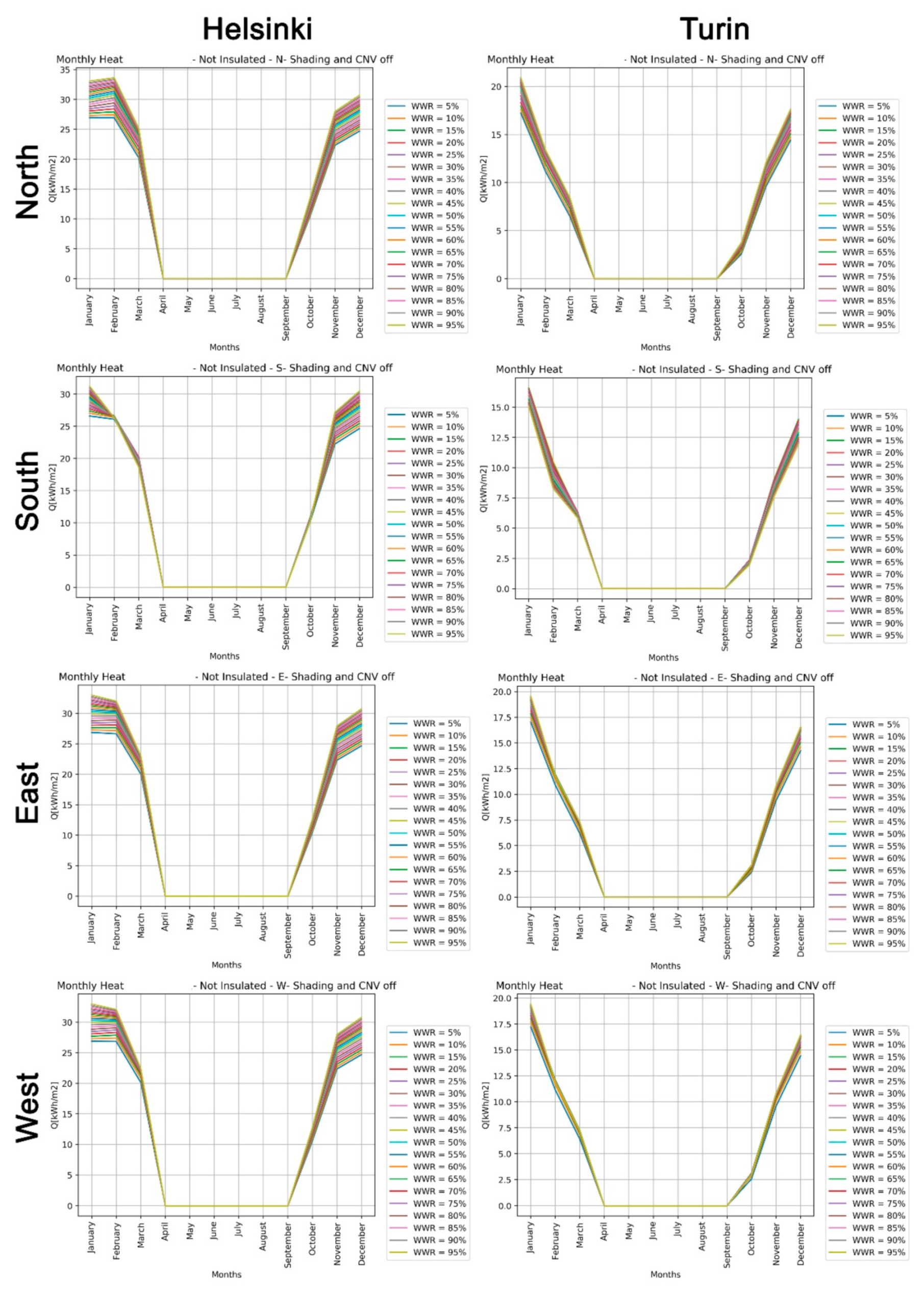
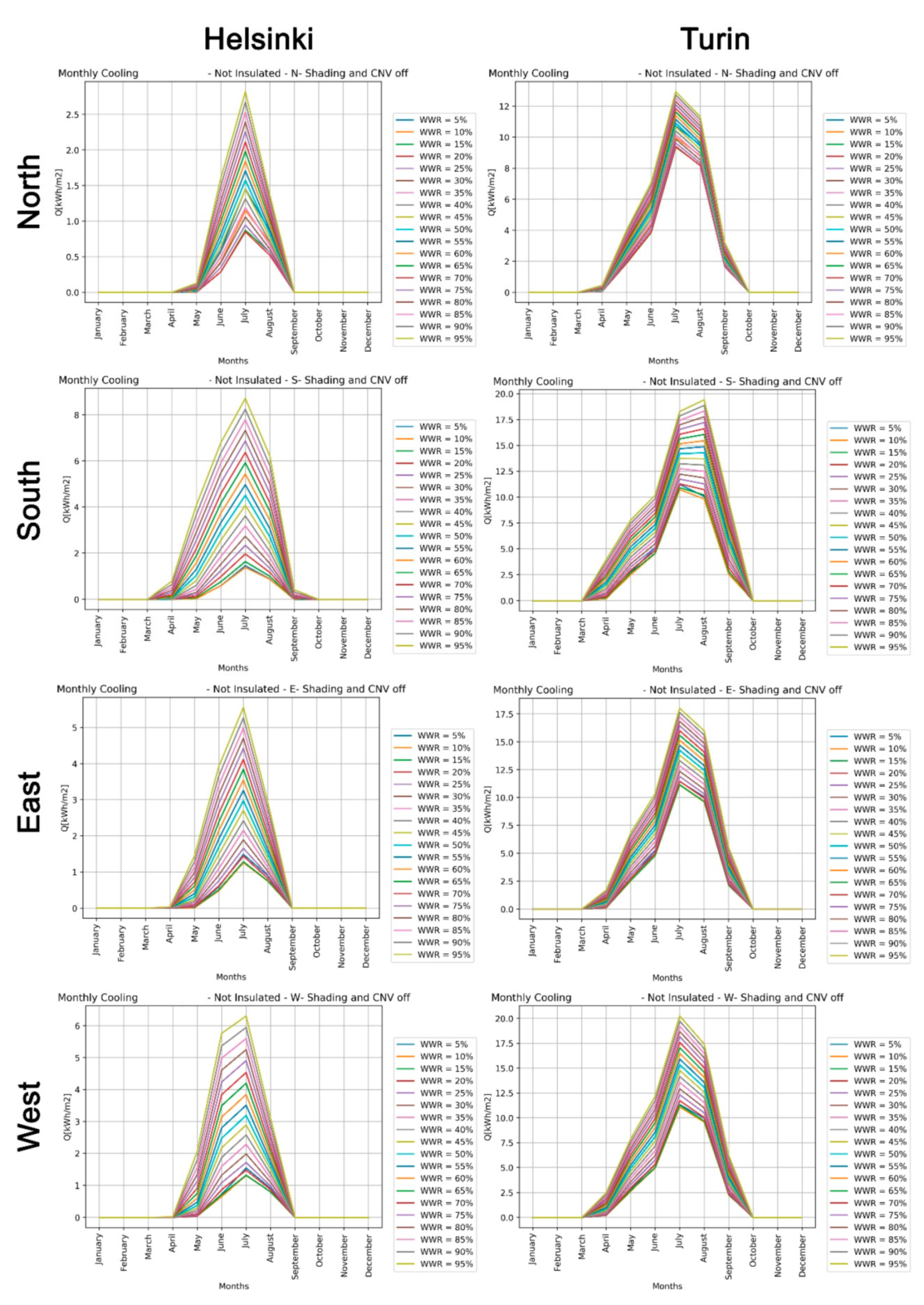
  • As expected, in the absolute values, the energy needs are always higher with lower insulation levels for any window orientation; the lowest amount of energy needs for each insulation level is reached with a Southern window orientation, whereby it is easier to reduce solar radiation in summer while solar gains contribute to space heating in winter.
  • Energy needs decrease with increasing WWR up to a certain %, with changes depending on both window orientation and insulation level.
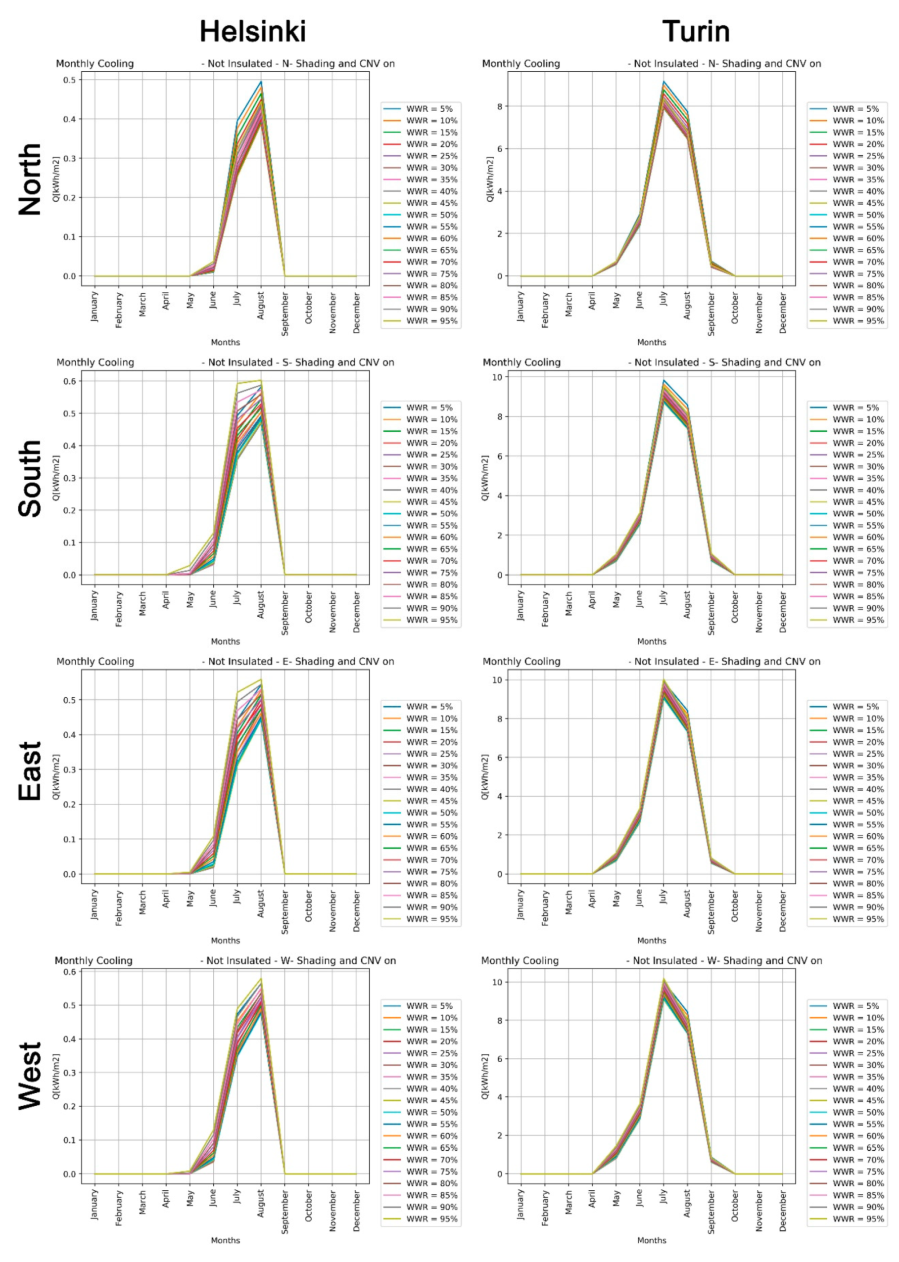
  • If a window is shaded, this trend inversion occurs in the range of 60% to 90%, due to a negative solar gains unbalance between winter and summer, in absence of heat dissipation by CNV; in fact, a shift of the trend inversion towards lower WWR values, and lower energy needs occur in the case of CNV on.
  • In the absence of shading, an abrupt decrease of energy needs occurs up to 20–50% of WWR, with an inversion of this trend afterword and always lower values if CNV is on; within the above-mentioned range, the minimum values are shifted towards higher values of WWR in the case of CNV on.
  • Considering a WWR around 30% as a common average value in the current building design practice, an optimal window configuration, corresponding to the lowest annual combined energy need, is given by the case with shading off and CNV on for all orientations.
The graphs of Figure 7 and Figure 8 show that the higher the WWR, the lower the lighting energy needs due to increased daylight, while it increases the risk of summer overheating. In winter, the increase in solar gains due to a larger window is counterbalanced, in almost all cases, by an increase of thermal losses, due to the higher-value of glazing in respect to opaque walls.
The graphs (a) in Figure 7 and Figure 8 refer to the North position, in which the window receives little or no direct solar radiation, while graphs (b) are related to the window exposed towards South, intercepting solar radiation during the hours when it is most energy intensive. Considering the South and North facing windows, the cases of Helsinki and Turin are differentiated, as expected, by higher values of energy needed for heating and much lower values for cooling in the former location, while lighting energy needs are similar in both cases. Heating energy need, which is not dependent of shading and CNV in both locations and orientations, is affected by WWR for the North-oriented window, according to the trend of a continuous increase in Helsinki and up to 60% WWR, with an almost constant trend afterword, in Turin. For the South-oriented window, heating energy need increases up to 25% WWR in Helsinki, and 15% WWR in Turin; above those values, an abrupt change in trend occurs with a continuous decrease. Regarding cooling energy needs, which are negligible in Helsinki for a North-facing window, shading is the most affecting condition with an abrupt change in trend from a decrease to increase of energy need at 10% WWR in both locations for a non-shaded South-oriented window. The addition of shading in the South-oriented window has an effect of keeping the cooling energy need almost constant with WWR in Turin, while increases above 30% WWR in Helsinki. Combining shading and opening for CNV in the South-oriented window, practically zeros cooling energy in Helsinki and lower it to a negligible value in Turin.
Regarding graphs (c)—East-oriented window—and (d)—West-oriented window—in the case of Helsinki, the trend of heating energy need is similar to the one of the North-facing window, while the trends of cooling energy are similar to the ones of the South-facing window. In Turin, the trend of heating energy need is similar to the one of the South-facing window, but with a shift of the inversion peak to 40% and 35% WWR for East and West orientation, respectively; while the trends of cooling energy need are similar to the ones of the South-facing window.
The energy need for lighting decreases continuously with WWR by a non-linear trend in both locations and it is affected only slightly by the shading condition, more so in Turin than in Helsinki.
Since lighting energy needs are particularly high in office buildings, they have a significant impact on the definition of the optimal WWR configuration. In fact, a reduction of WWR, which could increase energy efficiency if only heating and cooling needs were taken into account, would not have the same effect if considering lighting energy needs as well.

4. Discussion

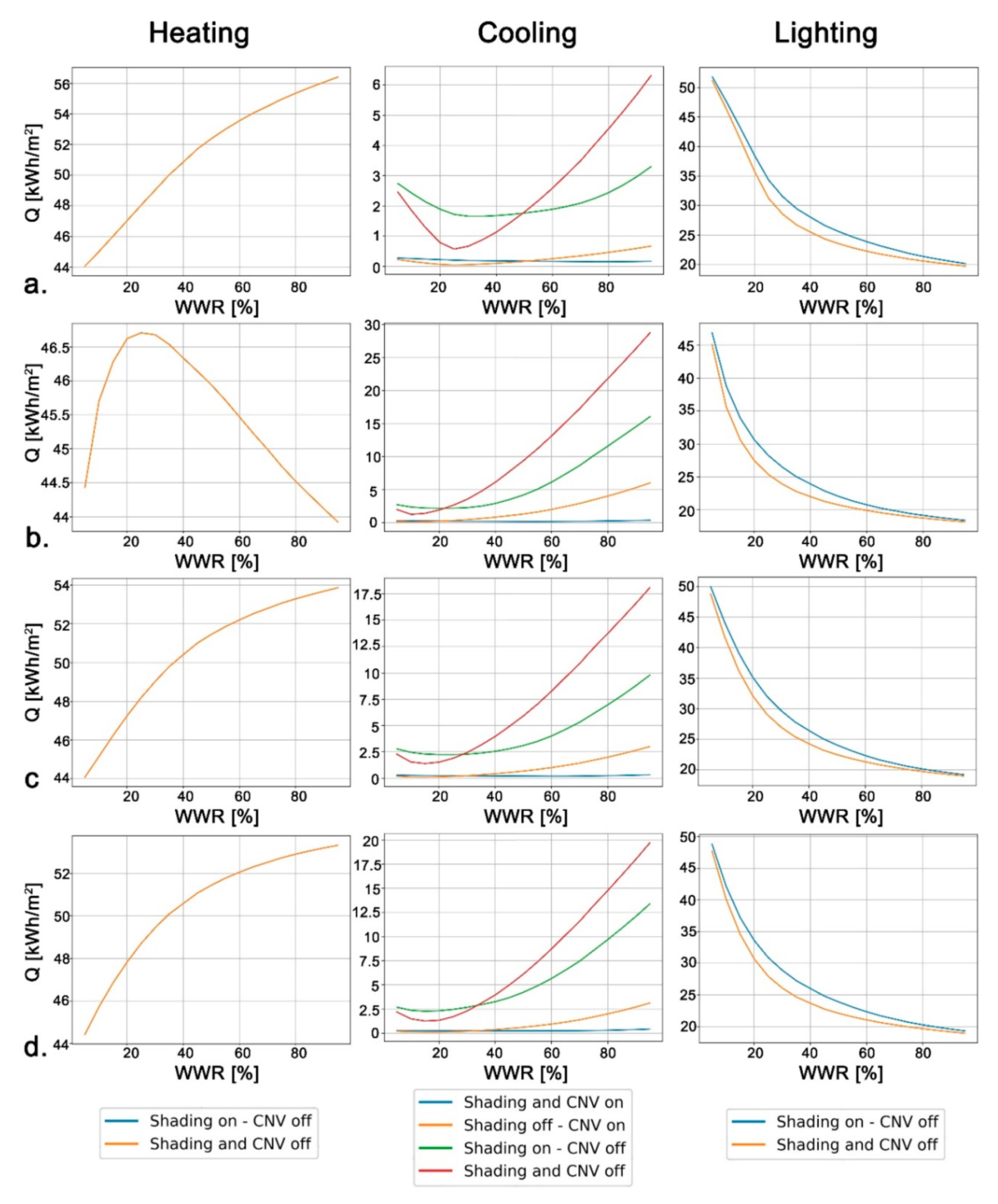
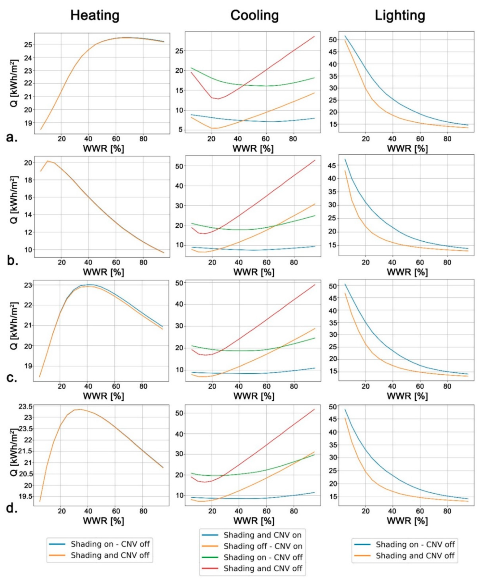
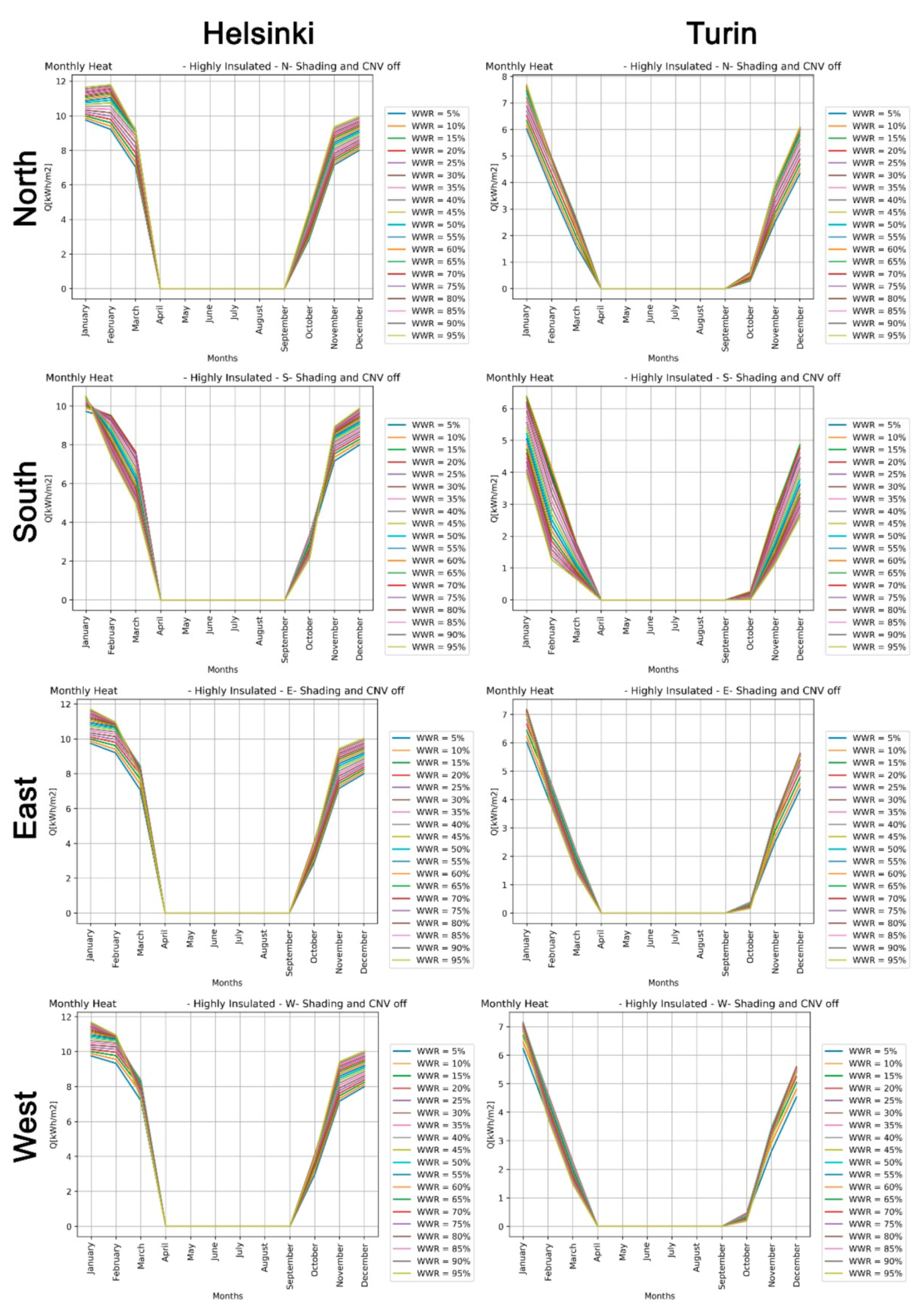
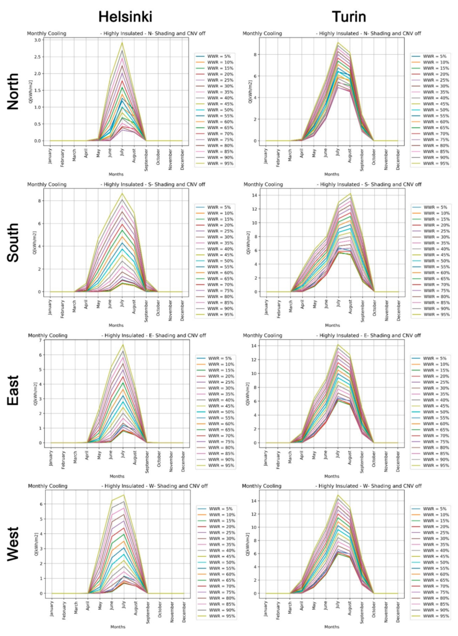
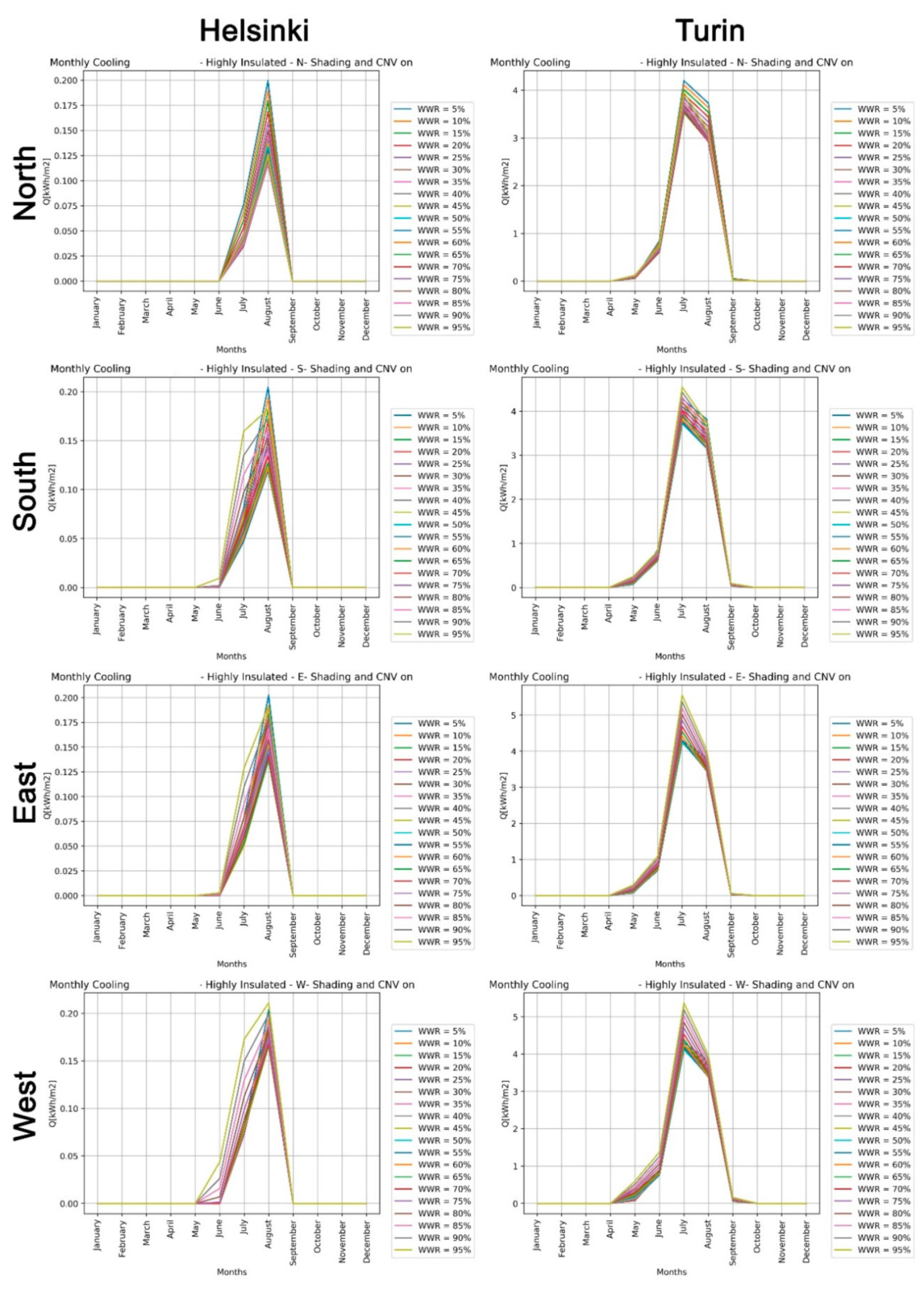
4.1. Monthly Energy Needs

The monthly energy need distribution as a dependent variable of WWR for each considered window shading/opening configuration allows for a more detailed assessment of the simulation results. These data are shown in Figure 9 and Figure 10 for Helsinki and Turin, respectively, considering the heating and cooling needs—using a variation range of WWR by intervals of 5%. As the graphs show, the general trends follow the expected distributions: high heating values of energy needs during the winter season and low or equal to zero values during the summer, while an opposite trend is highlighted for cooling energy needs. However, it is possible to state that varying WWR has an effect on energy needs as described in the general comments of Figure 7 and Figure 8. Focusing on the high insulated scenario, in the heating season, the distribution of monthly energy needs shows that for colder months: low WWR are suitable, while during other winter months high WWR may perform better. This occurs mainly with the South-facing window and not with the North-facing one due to the almost null potential of solar gains—see Figure 9. For example, in the Helsinki South-facing case, the reversal between high and low WWR as an optimal configuration, occurs between January and February, and between October and November, in the high-insulated scenario. Differently, for the cooling season, when shading and CNV are not activated, high WWRs show the worst behaviour in all months—see Figure 10—while this trend is counterbalanced when CNV is activated.
When both shading and CNV systems are activated—see Figure 11—the monthly cooling energy needs decrease considerably due to the heat dissipation effect of ventilative cooling and the heat gain prevention of shading. Moreover, this effect is not only apparent in terms of the intensity of the cooling need, but also in the number of months where the cooling system has to be activated. In fact, as is shown in Figure 11, it is possible to underline that these passive cooling systems may almost nullify the cooling needs in the Helsinki case, passing from a peak of about 8.5 kWh/m2 (WWR 95%) for the South façade, to a peak of 0.2 kWh/m2. Furthermore, the number of months interested by cooling needs, drastically reduces. Similarly, in the Turin case, the effect of shading and ventilative cooling more than half the cooling energy needs in all façade orientations. For the south façade case, in particular, cooling needs decrease from about 14.2 kWh/m2 to about 6 kWh/m2 (WWR 95%). Considering the number of cooling months, a reduction from the April-September period in the case without passive solutions, and May/June-August period with these counteractions (south-façade) is evident.
This could be explained by the greenhouse effect happening during daylight hours, especially for the highly insulated scenario. The differences between Helsinki and Turin, in term of cooling intensity and number of months when cooling is needed, are related to local climate characteristics. In a temperate climate such as Turin’s, overheating may occur also in winter months, particularly in high insulated buildings [38]. CNV and shading do not affect heating needs due to the adopted activation thresholds, except for a very little impact in some spring and fall months.
When the non-insulated scenario is considered, the general heating and cooling energy trends are comparable to the ones of the high-insulated building, but with a difference in absolute energy intensity values—see Figure 12 and Figure 13. Nevertheless, small changes may be found for cooling energy needs in the case of CNV and shading—see Figure 14—as demonstrated by the results of the annual analysis—see Figure 7 and Figure 8.

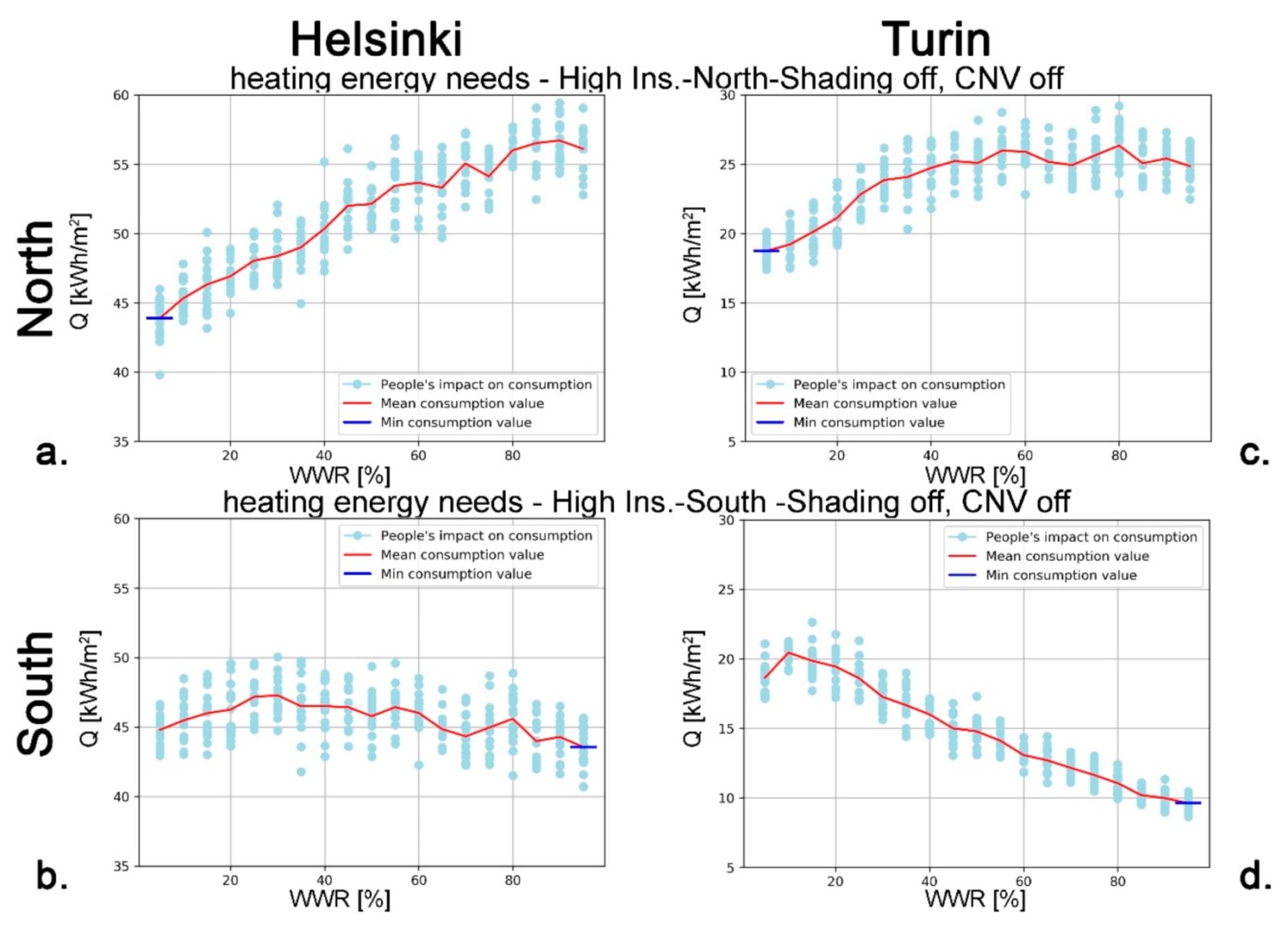
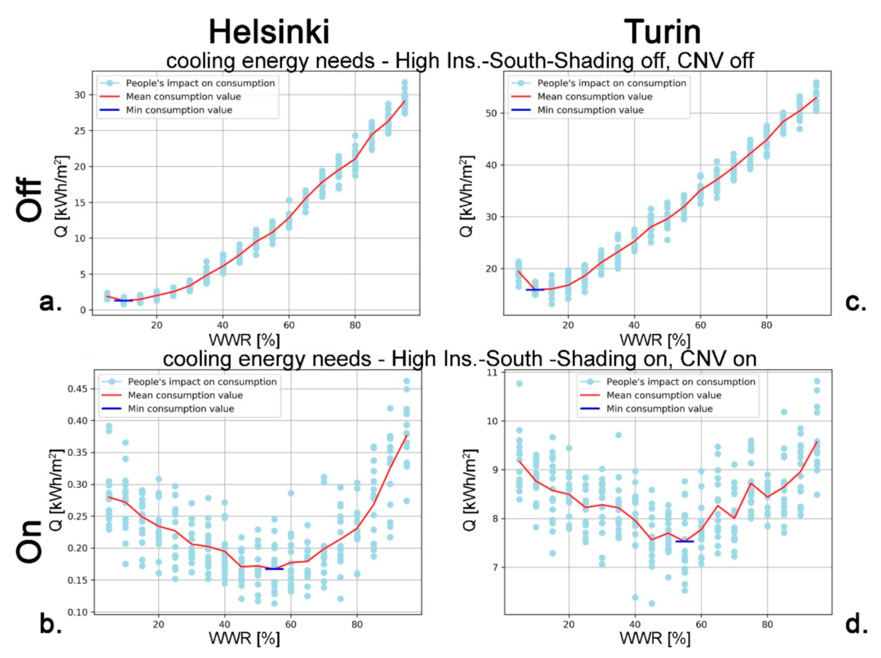
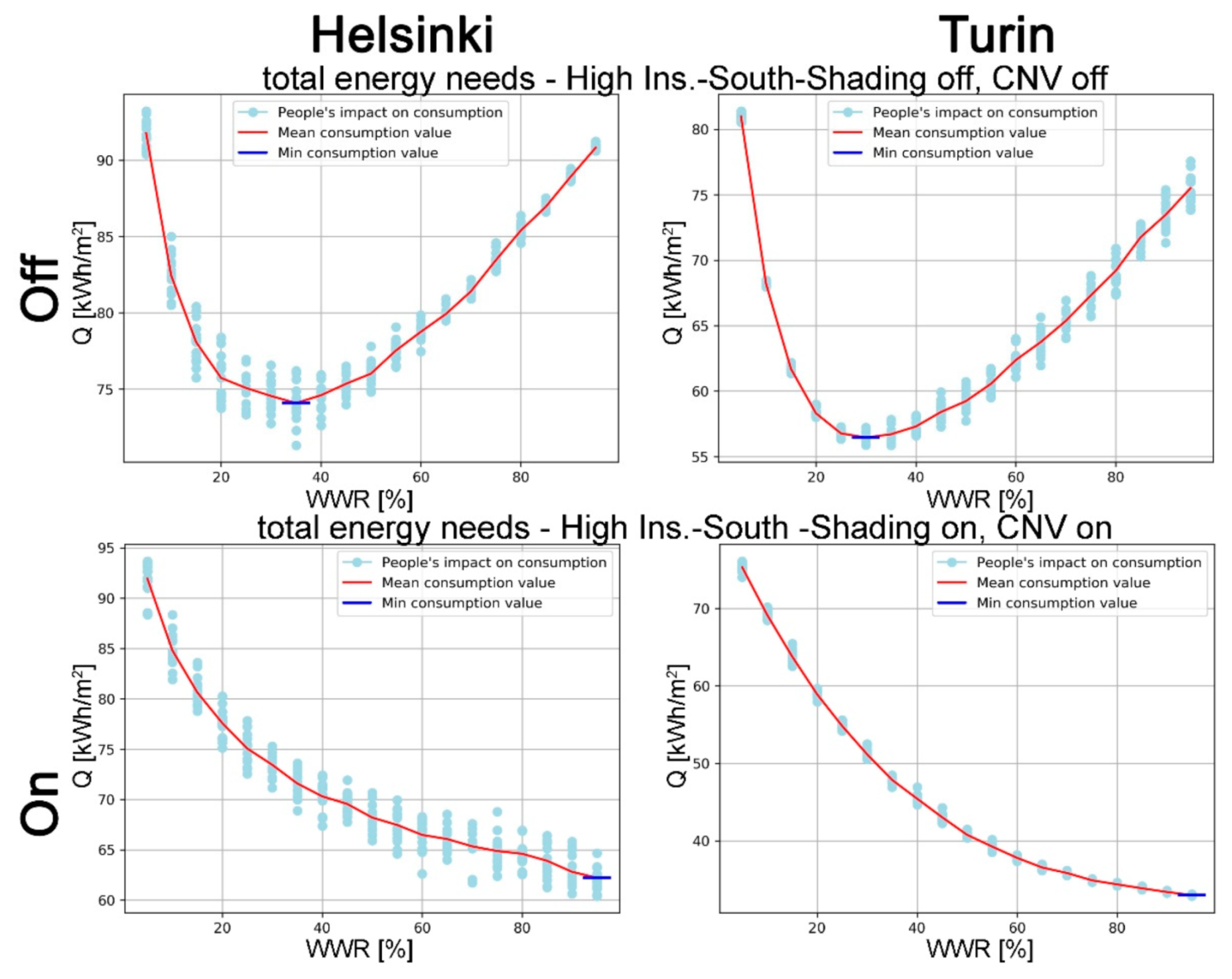
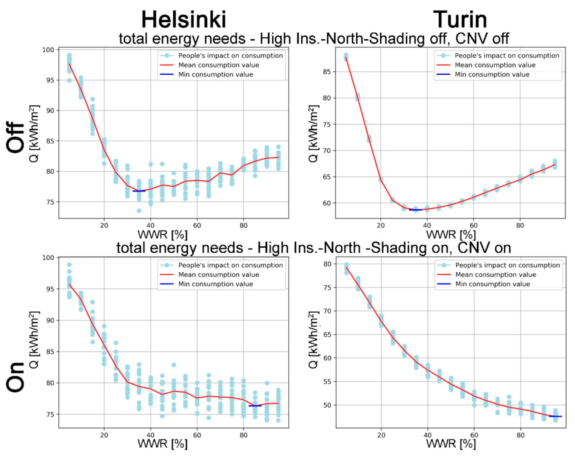
4.2. Sensibility Analysis by Changing the Occupancy Value

In this section, the methodology and results of a sensibility analysis carried out with the changing occupancy rate dynamically in every simulation are described in order to evaluate the impact of the random presence of people on energy needs. Based on the daily schedule of an office building, or general occupancy, each simulation was performed, inputting a random value of people density derived from a Gaussian distribution, G(μ,σ), and assuming mean and variance values as described in the methodological Section 2. Hence, combining all variables as described in Table 1, a total of 48 cases for each location, resulting in 16,128 simulations were carried out.
Some results, expressed as the total energy needs as a function of WWR, are shown in Figures 17 and 18, in relation to the following configurations.
Heating season:
  • Insulation scenario: Highly Insulated
  • Exposure: South; North
  • Shading and CNV Setup: both “Off”
Cooling season:
  • Insulation scenario: Highly Insulated
  • Exposure: South
  • Shading and CNV Setup: both “Off; both “On”
For each value of WWR, 16 different values of energy need intensity [kWh/m2] were calculated by assuming relevant random occupancy variations. As expected, an increase in the number of people led to a decrease of heating energy need and to an increase of cooling need. Nevertheless, the decrease of heating energy need is not as sharp as the increase of the cooling need, partially due to the clothing schedule used in the software.
The energy need for lighting does not have any random variation but is related to the illuminance requirement set for an office and relevant schedule.

4.2.1. Heating Energy Need

Figure 15 reports the heating energy needs for Helsinki and Turin for the 2 defined configurations (North and South facing window). In both cases, the heating energy need is highly influenced by the occupancy variation, depending on the relevant internal gain variation; this is more apparent for Helsinki due to the lower ambient temperature. Nevertheless, after an initial negative effect, when an increase of the average façade U-value is not sufficiently balanced by an increase of solar gains, the increment of WWR allows for reducing the heating demand. This is true for Turin, due to temperate climate conditions, while it is less apparent in Helsinki, in line with other studies [26]. When the window is facing north, the smallest values of heating energy needs correspond to the lowest WWR in both Helsinki and Turin, due to the limited amount of solar gains reaching north-facing façades in winter.

4.2.2. Cooling Energy Need

Cooling energy needs increase with WWR in both locations when CNV and shading are not activated—see Figure 16. Their trend is similar in both locations, while their absolute intensity values are remarkably different due to local climate conditions. When switching “On” both shading and CNV, the energy need decreases considerably until about 55% of WWR in both locations. After this value, the cooling need start to grow again because the cooling effect of CNV and shading is not sufficient to counterbalance the heat due to solar and internal gains. Roughly speaking, the average trends are similar to the ones shown in Figure 9 and Figure 10, even if the effect of random occupancy on the internal heat gain may slightly alter the results. Nevertheless, the random presence of people does not vary so much the cooling energy needs for each WWR in comparison to its effect in the heating season (CNV and shading set to Off)—the cooling variance is, in fact, smaller than in the heating case.

4.2.3. Total Energy Needs
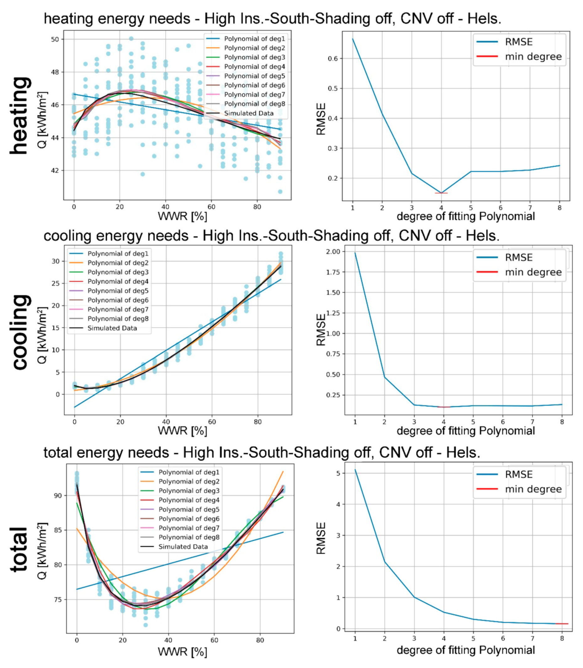
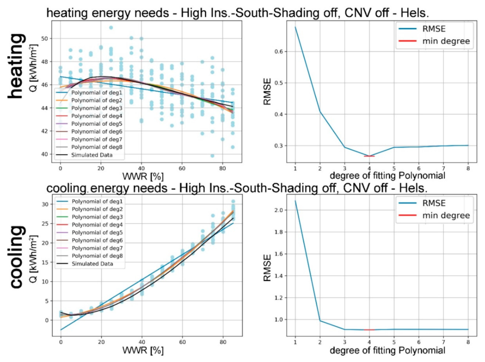
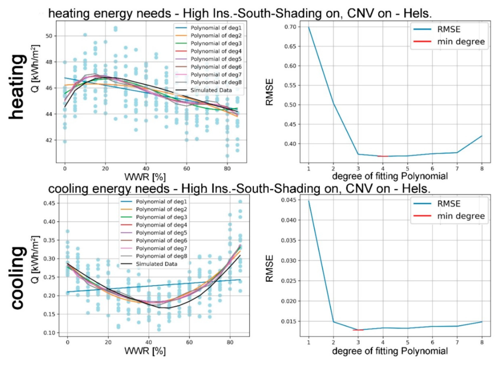
If CNV and shading are off, the optimum WWR for a South-facing window, corresponding to the lowest energy need, is reached between 35–40% for Helsinki and at about 30% in Turin, considering the random occupancy effect—see Figure 17. The ventilative cooling effect in reducing the cooling needs as well as the shading effect in preventing the solar gains are apparent both in Helsinki and Turin, with differences related to the local impact of cooling loads, higher in Turin than in Helsinki. When CNV and shading are activated, the highest WWR corresponds to the lowest energy need in both cases due to the possibility of balancing summer overheating without compromising the positive effect of winter solar gain. In fact, thanks to the local climate conditions of the considered locations, summer outdoor air temperatures are sufficiently lower than both the indoor and the comfort threshold temperatures.
If CNV and shading are off, the optimum WWR for a North-facing window is reached between 35–40% for both Helsinki and Turin—see Figure 18. Even in this case, the positive effect of shading and CNV in reducing the cooling demand is apparent. In particular, for Helsinki the optimal WWR is reached for values around 85%, while for Turin, values around 95% are suggested. This difference is due to the yearly balance between heating and cooling energy needs according to local climate conditions.

4.3. Regression

Starting from the number of points derived from the simulations, a dataset was built in order to fit a model that could predict the energy need based on WWR. An assumption is made that those points are the independent variables (predictors), with values varying at every 5% interval, and as a dependent variable the energy need intensity Q (kWh/m2). The polynomial curve fitting method implemented in the Numpy Python library was used as regression technique. This technique approximates the process of constructing a curve, or a mathematical function that has the best fit to a series of data points. This technique works in both the case in which data on the y axis has shape (1,1) and the case where shape is (N,1). Here, N = 16. A number of alternative curves, with a degree of the polynomial fitting ranging from 1 to 6, were then elaborated and the relevant RMSE (root mean square error) calculated.
The RMSE values are useful to select the best fitting curve, i.e., choosing a polynomial degree avoiding both underfitting and overfitting problems. If the degree of the fitting curve is too low—underfitting—then the fitting curve is missing important features, while if the degree is too high—overfitting—then the fitting curve is also modelling noise.
The formula used to calculate the RMSE is the following, where predicted and target are N-dimensional vectors.
RMSE = (mean((predicted-target)2)0.5
The RMSE was calculated by comparing the mean of the Gaussian distribution, from which the values used for getting the random occupancy points was derived (test set), against the curve derived from varying the WWR while keeping the occupation density constant—no added random noise—(training set). The obtained RMSE can be considered as an evaluation of the similarity of the regressed curve over the training set, because the energy need for these WWR values was known since they had been simulated.
In addition, for evaluating the accuracy of the regression model, it was also possible to simulate, for a specific setup, the heating and cooling energy needs for different values of WWR that were not considered in the training domain. This analysis was performed for the Helsinki case, even if the same method may be applied to different locations.

4.3.1. Regression over the Train Set

Regression analyses were not performed on the lighting energy need because random occupancy variations do not influence this specific value, being dependent on a fixed illuminance threshold and on the percentage of natural light passing through the window, but independent of the intensity of people present. Differently, cooling and heating energy needs are dependent on the random occupancy variation due to people internal gain production. Nevertheless, the analyses on the total energy needs are based on cooling, heating and lighting.
For the configurations shown in Figure 19, the polynomial degree that fits best the extracted points is 4 for both heating and cooling. On the contrary, for the total energy, the polynomial degree that fits best the extracted points is the highest—8—because of the behaviour of the dataset distribution.
As expected, the RMSE values are very small. In fact, the points used to fit the model and to perform the regression can be considered as noised values of the curves that we use to calculate the error. A test on an independent database is hence needed.

4.3.2. Regression over the Test Set

In this second test analysis, a prediction of energy needs for heating and cooling was elaborated, based on unknown values of WWR.
Starting from the model derived from the train dataset – WWR = [1, 5, 10, 15, …, 95]—a regression analysis on new test values—WWR = [2.5, 7.5, 12.5, …]—was carried out. As can be seen in Figure 20—with CNV and shading off, and in Figure 21 with CNV and shading on, energy needs are well predicted also when using other values of WWR. Comparing these values to the ones those derived from simulating the new values of WWR by EnergyPlus, the RMSE was calculated. As expected, this RMSE is a little bit higher than the RMSE of the training set, even if is still very low. The degree of the polynomial that better fits the points is again the fourth for the heating and the cooling cases.
In Table 5 and Table 6, the values of RMSE for the training and testing of cooling and heating energy are shown.

5. Conclusions

The analyses presented in this paper help to characterize, through hourly-based dynamic simulations, the influence of the window-to-wall ratio (WWR) on the energy need for space heating and cooling, and the lighting of an office building in two reference locations representing a cold and a moderate climate zone of Europe. Various envelope and window characteristics were considered as independent variables, namely: insulation level, orientation, shading, controlled natural ventilation.
Results of simulations at constant occupation rate show that an optimal WWR value, balancing the three above-mentioned energy uses in terms of the least energy annual need, can be found around 30% for both locations.
A second type of study dealt with a regression analysis of data resulting from simulations carried out by an algorithm developed for the purpose of allowing a changing occupation rate based on random behaviour. This analysis aimed to simulate the reference case conditions in the way closest to the actual dynamic context. In addition, several regression curves and the relevant RMSE were yielded and compared in order to find the correlation factor which could best fit the analysed data sets.
In general, the analyses carried out have a methodological value in representing an innovative approach to define the optimal configurations of building envelopes and window characteristics with respect to the minimization of annual energy needs. Furthermore, this study’s purpose is consistent with the minimum requirements of a passive house and includes the potential effects of random variation in occupancy. This approach allows for supporting design choices from the preliminary phase while considering perturbation phenomena that may occur in real situations.

Author Contributions

Article conceptualization, G.C.; methodology, G.C., A.A.; software, L.B., M.F., E.P., E.S.; investigation, G.C., M.F., E.P., E.S.; writing—original draft preparation, G.C., M.F., E.P., E.S.; writing—review and editing, G.C., M.G.; supervision, G.C., with A.A., M.G.; funding acquisition, G.C.

Funding

The research was co-funded by the 59_ATEN_RSG16CHG.

Acknowledgments

The proposed approach was tested during the Course ICT in Building Design, Master Degree in ICT for Smart Society, Politecnico di Torino, Italy, A.Y. 2018-19, with the support of the LASTIN laboratory, Microclimate section.

Conflicts of Interest

The authors declare no conflict of interest. The funders had no role in the design of the study; in the collection, analyses, or interpretation of data; in the writing of the manuscript, or in the decision to publish the results.

Nomenclature

WWRWindows-to-Wall Ratio
VCVentilative Cooling
CNVControl Natural Ventilation
RMSERoot Mean Square Error
DBDesign Builder software

References

  1. Orme, M. Estimates of the energy impact of ventilation and associated financial expenditures. Energy Build. 2011, 33, 199–205. [Google Scholar] [CrossRef]
  2. Cuce, P.M.; Riffat, S. A state of the art review of evaporative cooling systems for building applications. Renew. Sustain. Energy Rev. 2016, 54, 1240–1249. [Google Scholar] [CrossRef]
  3. Logue, J.M.; Sherman, M.H.; Walker, I.S.; Singer, B.C. Energy impacts of envelope tightening and mechanical ventilation for the U.S. residential sector. Energy Build. 2013, 65, 281–291. [Google Scholar] [CrossRef] [Green Version]
  4. European Commission. Communication from the Commission to the European Parliament, the Council, the European Economic and Social Committee, the Committee of the Regions and the European Investment Bank, Clean Energy for All Europeans; COM(2016) 860 Final; European Commission: Brussels, Belgium, 2016. [Google Scholar]
  5. Santamouris, M. (Ed.) Advances in Passive Cooling; Earthscan: London, UK, 2007; ISBN 978-1-84407-263-7. [Google Scholar]
  6. Santamouris, M.; Asimakopolous, D. (Eds.) Passive Cooling of Buildings; James & James: London, UK, 1996; ISBN 1-873936-47-8. [Google Scholar]
  7. IEA. The Future of Cooling. Opportunities for Energy Efficient Air Conditioning; International Energy Agency: Paris, France, 2018. [Google Scholar]
  8. Kolokotroni, M.; Heiselberg, P. (Eds.) Ventilative Cooling State of the Art; International Energy Agency—Energy in Buildings and Communities Programme, Aalborg University: Aalborg, Denmark, 2015; ISBN 87-91606-25-X. [Google Scholar]
  9. Grosso, M.; Acquaviva, A.; Chiesa, G.; da Fonseca, H.; Bibak Sareshkeh, S.S.; Pardilla, M.J. Ventilative cooling effectiveness in office buildings: A parametrical simulation. In Proceedings of the 39th AIVC—7th TightVent & 5th Venticool Conference, Antibes Juan-Les-Pins, France, 18–19 September 2018; AIVC-INIVE: Brussels, Belgium, 2019; pp. 780–788. [Google Scholar]
  10. Chiesa, G.; Grosso, M.; Pearlmutter, D.; Ray, S. Editorial. Advances in adaptive comfort modelling and passive/hybrid cooling of buildings. Energy Build. 2017, 148, 211–217. [Google Scholar] [CrossRef]
  11. Santamouris, M. Cooling the buildings—Past, present and future. Energy Build. 2016, 28, 617–638. [Google Scholar] [CrossRef]
  12. Goia, F.; Haase, M.; Perino, M. Optimizing the configuration of a façade module for office buildings by means of integrated thermal and lighting simulations in a total energy perspective. Appl. Energy 2013, 108, 515–527. [Google Scholar] [CrossRef]
  13. Arumi, F. Day lighting as a factor in optimizing the energy performance of buildings. Energy Build. 1977, 1, 175–182. [Google Scholar] [CrossRef]
  14. Johnson, R.; Sullivan, R.; Selkowitz, S.; Nozaki, S.; Conner, C.; Arasteh, D. Glazing energy performance and design optimization with daylighting. Energy Build. 1984, 6, 305–317. [Google Scholar] [CrossRef] [Green Version]
  15. Baker, N.V.; Steemers, K. LT Method 3.0—A strategic energy-design tool for Southern Europe. Energy Build. 1996, 23, 251–256. [Google Scholar] [CrossRef]
  16. Su, X.; Zhang, X. Environmental performance optimization of window-wall ratio for different window type in hot summer and cold winter zone in China based on life cycle assessment. Energy Build. 2010, 42, 198–202. [Google Scholar] [CrossRef]
  17. Ma, P.; Wang, L.-S.; Guo, N. Maximum window-to-wall ratio of a thermally autonomous building as a function of envelope U-value and ambient temperature amplitude. Appl. Energy 2015, 146, 84–91. [Google Scholar] [CrossRef]
  18. Lee, J.W.; Jung, H.J.; Park, J.Y.; Lee, J.B.; Yoon, Y. Optimization of building window system in Asian regions by analysing solar heat gain and daylighting elements. Renew. Energy 2013, 50, 522–531. [Google Scholar] [CrossRef]
  19. Kheir, F. The relation of orientation and dimensional specifications of window with building energy consumption in four different climates of Köppen classification. Researcher 2013, 5, 107–115. [Google Scholar]
  20. Goia, F. Search for the optimal window-to-wall ration in office buildings in different European climates and the implications on total energy saving potential. Sol. Energy 2016, 132, 467–492. [Google Scholar] [CrossRef]
  21. Košir, M.; Gostiša, T.; Kristl, Z. Influence of architectural building envelope characteristics on energy performance in Central European climatic conditions. J. Build. Eng. 2017, 15, 278–288. [Google Scholar] [CrossRef]
  22. Echenagucia, T.M.; Capozzoli, A.; Cascone, Y.; Sassone, M. The early design stage of a building envelope: Multi-objective search through heating, cooling and lighting energy performance analysis. Appl. Energy 2015, 154, 577–591. [Google Scholar] [CrossRef]
  23. Consumption of Buildings. A parametric analysis in Italian climate conditions. J. Build. Eng. 2017, 13, 169–183. [Google Scholar] [CrossRef]
  24. Alghoul, S.K.; Rijabo, H.G.; Mashena, M.E. Energy consumption in buildings: A correlation for the influence of window to wall ratio and window orientation in Tripoli, Libya. J. Build. Eng. 2017, 11, 82–86. [Google Scholar] [CrossRef]
  25. Wen, L.; Hiyama, K.; Koganei, M. A method for creating maps of recommended window-to-wall ratios to assign appropriate default values in design performance modeling: A case study of a typical office building in Japan. Energy Build. 2017, 145, 304–317. [Google Scholar] [CrossRef]
  26. Feng, G.; Chi, D.; Xu, X.; Dou, B.; Sun, Y.; Fu, Y. Study on the Influence of Window-wall Ratio on the Energy Consumption of Nearly Zero Energy Buildings. Procedia Eng. 2017, 205, 730–737. [Google Scholar] [CrossRef]
  27. Sun, Y.; Shanks, K.; Baig, H.; Zhang, W.; Hao, X.; Li, Y.; He, B.; Wilson, R.; Liu, H.; Sundaram, S.; et al. Integrated CdTe PV gazing into windows: Energy and daylight performance for different window-to-wall ratio. Energy Procedia 2019, 158, 3014–3019. [Google Scholar] [CrossRef]
  28. Xue, Q.; Li, Q.; Xie, J.; Zhao, M.; Liu, J. Optimization of window-to-wall ratio with sunshades in China low latitude region considering daylighting and energy saving requirements. Appl. Energy 2019, 233–234, 62–70. [Google Scholar] [CrossRef]
  29. Chiesa, G.; Grosso, M. An Environmental Technological Approach to Architectural Programming for School Facilities. In Mediterranean Green Buildings & Renewable Energy; Sayigh, A., Ed.; Spinger: Cham, Switzerland, 2017; pp. 701–716. [Google Scholar] [CrossRef]
  30. Passive House Institute. Available online: https://passivehouse.com/index.html (accessed on 10 May 2019).
  31. Chiesa, G.; Grosso, M.; Acquaviva, A.; Makhlouf, B.; Tumiatti, A. Insulation, building mass and airflows provisional and multivariable analysis. Sustain. Mediterr. Constr.—SMC 2018, 8, 36–40. [Google Scholar]
  32. The British Council for Offices. Occupier Density Study 2013; BCO: London, UK, 2013. [Google Scholar]
  33. Grosso, M. (Ed.) Il raffrescamento passivo degli edifici, 2nd ed.; Maggioli: Sant’Arcangelo di Romagna, Italy, 2008; p. 313. ISBN 978-88-387-3963-3. [Google Scholar]
  34. Olgyay, A.; Olgyay, V. Solar Control and Shading Devices; Princeton University Press: Princeton, NJ, USA, 1957. [Google Scholar]
  35. U.S. Department of Energy. EnergyPlus™ Version 8.9.0 Documentation. Engineering Reference; U.S. Department of Energy: Washington, DC, USA, 2018.
  36. Watson, D.; Labs, K. Climatic Design. Energy-Efficient Building Principles and Practices; McGraw-Hill: New York, NY, USA, 1983; ISBN 0-07-068478-2. [Google Scholar]
  37. Mazria, E. The Passive Solar Energy Book; Rodale: Emmaus, PA, USA, 1979; ISBN 0-87857-237-6. [Google Scholar]
  38. Heiselberg, P. (Ed.) Ventilative Cooling Design Guide; IEA EBC Annex 62; Aalborg University Press: Aalborg, Denmark, 2018; ISBN 87-91606-38-1. [Google Scholar]
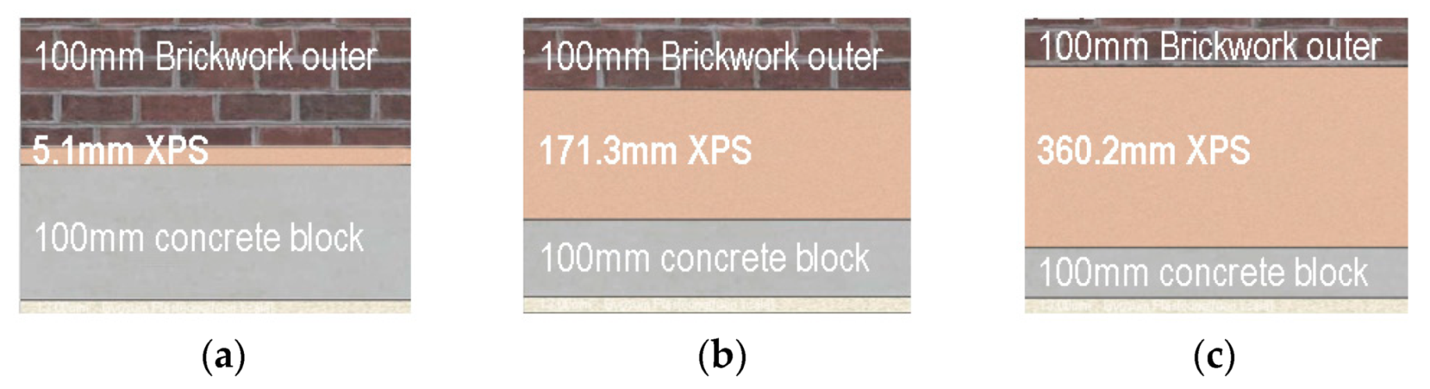
Figure 1. Sample plot of 10,000 random occupancy values generated by the used Gaussian model – total office area = 80 m2.
Sustainability 11 03078 g001
Figure 2. Sketch of the developed simulation engine.
Sustainability 11 03078 g002
Figure 3. Visualization of (a) the reference office unit (open office room + corridor), and (b) its virtual position in a multi-storey building.
Sustainability 11 03078 g003
Figure 4. Layers and materials for the 3 configurations of opaque envelope: (a) Low insulation (almost null), (b) Medium insulation, (c) High insulation.
Sustainability 11 03078 g004
Figure 5. Annual energy need as a function of WWR for various envelope configurations—Helsinki case.
Sustainability 11 03078 g005
Figure 6. Annual energy need as a function of WWR for various envelope configurations—Turin case.
Sustainability 11 03078 g006
Figure 7. Heating, Cooling, and lighting annual energy needs as a function of WWR for different setting of shading and CNV as well as window orientations in the high insulation scenario, in Helsinki: (a) North; (b) South; (c) East; (d) West.
Sustainability 11 03078 g007
Figure 8. Heating, Cooling, and lighting annual energy needs as a function of WWR for different setting of shading and CNV as well as window orientations in the high insulation scenario, in Turin: (a) North; (b) South; (c) East; (d) West.
Sustainability 11 03078 g008
Figure 9. Monthly distribution of the heating energy needs with Shading and CNV “Off”—high insulated scenario.
Sustainability 11 03078 g009
Figure 10. Monthly distribution of the cooling energy needs with Shading and CNV “Off”—high insulated scenario.
Sustainability 11 03078 g010
Figure 11. Monthly distribution of the cooling energy needs with Shading and CNV “On”—high insulated scenario.
Sustainability 11 03078 g011
Figure 12. Monthly distribution of the heating energy needs with Shading and CNV “Off”—not-insulated scenario.
Sustainability 11 03078 g012
Figure 13. Monthly distribution of the cooling energy needs with Shading and CNV “Off”—not-insulated scenario.
Sustainability 11 03078 g013
Figure 14. Monthly distribution of the cooling energy needs with Shading and CNV “On”—not-insulated scenario.
Sustainability 11 03078 g014
Figure 15. Heating energy needs for the highly insulated building, CNV and Shading off—for Helsinki (a) North-facing case; (b) South-facing case; and for Turin (c) North-facing case; (d) South-facing case.
Sustainability 11 03078 g015
Figure 16. Cooling energy needs for the highly insulated building, South-facing case—for Helsinki (a) CNV and shading off; (b) CNV and shading on; and for Turin (c) CNV and shading off; (d) CNV and shading on.
Sustainability 11 03078 g016
Figure 17. Total energy needs for a highly insulated building, South, Shading and CNV “On-Off”.
Sustainability 11 03078 g017
Figure 18. Total energy needs for a highly insulated building, North, Shading and CNV “On-Off”.
Sustainability 11 03078 g018
Figure 19. Figure 17—Heating, Cooling, Total regressed energy needs, with the corresponding RMSE for each degree (training).
Sustainability 11 03078 g019
Figure 20. Heating and Cooling regressed energy needs, with the corresponding RMSE for each degree (testing case)—CNV and shading off setup.
Sustainability 11 03078 g020
Figure 21. Heating and Cooling regressed energy needs, with the corresponding RMSE for each degree (testing case)—CNV and shading on setup.
Sustainability 11 03078 g021
Table 1. Insulation levels of the opaque envelope components (external wall and roof).
ConfigurationU-Value Walls [W/m2]U-Value Roof [W/m2]
Low insulation (non-insulated)1.51.5
Medium insulation0.180.18
High insulation0.090.09
Table 2. Insulation levels of windows and relevant materials.
ConfigurationGlass TypeU-value Windows [W/m2]
Low insulation (non-insulated)Single glazing, clear5.7
Medium insulationDouble glazing, clear, LoE, argon-filled1.49
High insulationTriple glazing, clear, LoE, argon-filled0.78
Table 3. Optimal WWR [%] and related total energy needs [kWh/m2] for various envelope configurations. Helsinki case.
Non-insulated
North South East West
CaseWWRQ [kWh/m2]WWRQ [kWh/m2]WWRQ [kWh/m2]WWRQ [kWh/m2]
Shading and CNV on30175.0355161.1740172.0135171.84
Shading on, CNV off30176.8445164.1240174.0935174.40
Shading off, CNV on25170.4530161.4525168.6225168.12
Shading and CNV off25171.7220164.7820170.8420170.51
Medium-insulated
North South East West
CaseWWRQ [kWh/m2]WWRQ [kWh/m2]WWRQ [kWh/m2]WWRQ [kWh/m2]
Shading and CNV on30106.675594.3335103.7030103.77
Shading on, CNV off30107.713597.3430105.2830105.88
Shading off, CNV on25104.333595.2425102.4925101.93
Shading and CNV off25104.692598.7525104.4220103.67
High-insulated
North South East West
CaseWWRQ [kWh/m2]WWRQ [kWh/m2]WWRQ [kWh/m2]WWRQ [kWh/m2]
Shading and CNV on9576.799562.769573.429573.11
Shading on, CNV off7579.105572.135578.464579.57
Shading off, CNV on5576.17067.266074.556074.12
Shading and CNV off4077.473574.073578.363077.84
Table 4. Optimal WWR [%] and related total energy needs [kWh/m2] for various envelope configurations. Turin case.
Non-insulated
North South East West
CaseWWRQ [kWh/m2]WWRQ [kWh/m2]WWRQ [kWh/m2]WWRQ [kWh/m2]
Shading and CNV on70108.379087.8970105.9870105.59
Shading on, CNV off70116.268598.1070115.2465116.34
Shading off, CNV on30108.052599.9525109.4920110.51
Shading and CNV off25116.3325110.8325119.7020120.52
Medium-insulated
North South East West
CaseWWRQ [kWh/m2]WWRQ [kWh/m2]WWRQ [kWh/m2]WWRQ [kWh/m2]
Shading and CNV on6065.988542.556062.295562.93
Shading on, CNV off5573.936056.605072.684575.70
Shading off, CNV on3565.884053.833065.902566.33
Shading and CNV off3073.163066.982576.662076.71
High-insulated
North South East West
CaseWWRQ [kWh/m2]WWRQ [kWh/m2]WWRQ [kWh/m2]WWRQ [kWh/m2]
Shading and CNV on9547.839532.999546.129546.49
Shading on, CNV off9557.978047.867558.716562.50
Shading off, CNV on5050.134543.773552.123552.32
Shading and CNV off3558.633056.303063.222562.94
Table 5. RMSE Cooling for Training and Testing.
RMSE Cooling trainRMSE Cooling testDeg Train
High Ins N Shading and CNV on0.00760.12825
High Ins N Shading and CNV off0.10040.90494
Table 6. RMSE Heating for Training and Testing.
RMSE Heating TrainRMSE Heating testDeg Train
High Ins S Shading and CNV on0.24170.36766
High Ins S Shading and CNV off0.15000.26634

