A Responsive Pricing Grid Operator Sourcing from Competing Generators under Uncertain Supply and Demand

1
College of Business, Shanghai University of Finance and Economics, Shanghai 200433, China
2
Institute of Logistics Science and Engineering, Shanghai Maritime University, Shanghai 201306, China
*
Author to whom correspondence should be addressed.
Sustainability 2019, 11(15), 4061; https://0-doi-org.brum.beds.ac.uk/10.3390/su11154061
Submission received: 5 July 2019
/
Revised: 21 July 2019
/
Accepted: 24 July 2019
/
Published: 27 July 2019
(This article belongs to the Section Economic and Business Aspects of Sustainability)
Abstract
:Electricity supply chains involve more sources of uncertainty than typical production and manufacturing supply chains, owing to the intermittent nature of renewable energy generation. Therefore, it is critical but challenging to mitigate supply disruption risks by improving management methods. The extant literature has mainly investigated the sourcing strategies of manufacturers with price-taking suppliers. Where there is an option to source from multiple generators, including regular but unreliable generators and reliable backup generators, a flexible sourcing strategy is usually regarded as the best tactic for the grid operator. Our objective is to evaluate the costs and benefits of flexible sourcing and sole sourcing when generators are strategic price-setters. In this paper, we develop a Stackelberg game with wholesale prices contingent on the dominant grid operator’s sourcing strategy. We describe and analyze the resulting equilibriums under different scenarios. The results show that the grid operator does not necessarily benefit from a backup generator and that the flexible sourcing mode is not in fact optimal, except when the disruption ratio of the unreliable generator is medium and the penalty-sharing ratio of the unreliable generator is low. The model is applied to a numerical case study of a real-word electricity supply chain to illustrate the validity and effectiveness of the proposed conclusions.
1. Introduction
1.1. Background and Current Issues
At the beginning of the twenty-first century, rapid advances in science and technology led to a boom in various renewable energies, such as wind and solar, which now account for a substantial proportion of electricity generation. By the end of 2017, the proportion of renewable electricity in the European Union had reached 30%, of which wind and solar power accounted for 11.2% and 3.7%, respectively. Moreover, a report by the International Energy Agency analyzing and predicting the development of renewable energies and technologies from 2018 to 2023 pointed out that the share of renewable energy for global energy demand is expected to grow by one-fifth in the next five years, reaching 12.4% in 2023 (https://www.iea.org/renewables2018/). In fact, as early as 2015, Denmark met 100% of its electricity demand with wind power on some days of the year [1]. Overall, renewable sources of energy, such as wind and solar, will play a key role in the future energy landscape. Although renewable energies have a great number of advantages in environmental and economic terms, electricity enterprises in the supply chain face more managerial problems because of a unique characteristic of renewable energies: their intermittency.
From a practical perspective, one of the greatest challenges of utilizing renewable energies is averting intermittency, that is, reducing the uncertainty of renewable energy electricity supply [2,3]. As the risk of supply disruption increases, so does the threat of a major loss, and this threat has motivated many firms and researchers to explore how to build a more easily maintained electricity supply chain with renewable energies. According to previous research, making strategic decisions and managing strategic behaviors are efficient ways to alleviate these problems [4,5,6,7,8,9,10]. In the early stages of renewable energy management, Tang used observations of successful business cases to propose several mitigation strategies for coping with uncertain supply [7]. Recently, Snoeck et al. developed a methodology to evaluate the costs of disruptions and the value of the supply chain network mitigation options that are popular among electricity firms [11]. From these pragmatic studies, we find that an improvement in management can dramatically increase operational efficiency in the renewable energy supply chain. Therefore, this paper places great emphasis on a flexible supply base and on guiding firms to make optimal strategic sourcing decisions.
In May 2018, the State Energy Administration issued its Notice on the Requirements for Wind Power Construction and Management. The Notice points out that, from 2019, all newly approved centralized onshore and offshore wind power projects in the provinces (autonomous districts and municipalities) must be allocated and determined through competition. Therefore, in this paper, we regard the generators as rational decision-makers of wholesale price, and we analyze their optimal pricing behaviors under different sourcing modes of the power grid.
1.2. Research Innovations and Contributions
To date, electricity consumption has mainly been supplied by traditional energy (fossil oil) and renewable energy. The present study is inspired by the fact that three supply modes coexist in the electricity supply chain. First, a renewable energy generator with a varied but unreliable power supply (one that carries a risk of disruption due to intermittency) can be regarded as an unreliable generator. Nevertheless, the electricity supply still consists of renewable energy, because of its low-carbon and eco-friendly characteristics. Furthermore, recent investigators have found that 100% renewable energy electricity (100RElec) mixes can be achieved if energy savings are significant enough [12]. Some researchers have claimed that 100RElec may be achieved sooner than expected [13]. Second, it has been observed that traditional energy is much more stable than renewable energy. In some natural resource-poor countries and areas, traditional energy is the only way to generate electricity. Last but not least, most countries adopt a merging mode, generating electricity from traditional and renewable energy at the same time. Accordingly, researchers have shown interest in systems that consist of different types of generator: inflexible, flexible, and variable (or intermittent) [14]. This paper focuses on all these scenarios and discusses each of them in technical terms.
Recently, many scholars have studied pricing and sourcing strategies under different modes [15], while others have studied the profitability of using more expensive suppliers as backup in case of supply disruptions [8,16]. However, most existing studies have assumed that the electricity demand is certain, that generators are decision-takers, and that inventories are indispensable. Under these constraints, their results have confirmed that the grid operator should maintain a reliable supplier as a backup. In contrast, in the present study, we relax these constraints to discuss scenarios with uncertain supply and demand, and we treat generators as strategic decision-makers who decide the wholesale price.
After considering the practical operation of the electricity supply chain, we construct a one-period model with one grid operator and two generators. As well as pricing and ordering policies, we investigate sourcing selection, including (a) sole sourcing from a reliable generator (SR, such as the Southern China Power Grid), (b) sole sourcing from an unreliable generator (SU, such as the West Inner Mongolia Power Grid), and (c) flexible sourcing from both an unreliable generator and a reliable generator (FS, such as the Eastern China Power Grid and Shandong Power Grid). The reliable generator can act as a single supplier (mode (a)) or provide backup quantity to the grid operator when the sole unreliable generator cannot satisfy the demand for electricity (mode (c)). Since the unreliable generator may suffer sudden disruption or its output may not be able to fulfill the order, the grid operator will be punished for delayed deliveries to industrial users, which specifically include producing enterprises. In modes (b) and (c), when delayed deliveries occur, the unreliable generator bears the responsibility and must pay the penalty. There are two options for the grid operator: to accept the delayed deliveries with the penalty, or to mitigate the disruption by choosing a reliable generator as a backup. The choice is made according to the wholesale prices of the two generators.
A principal objective of this research is to investigate and optimize pricing strategies for the generators and sourcing strategies for the grid operator. We establish and provide insights into three operation modes. More specifically, three main questions are addressed in this paper: (1) Under multi-uncertainties, what pricing schemes should be offered by the generators? (2) How should the electricity supply chain members (the generators and the grid operator) collaborate in terms of penalty-sharing contracts? (3) Which sourcing strategy (i.e., Sole Reliable, Sole Reliable, or Flexible Sourcing) could increase the generators’ profits when they strategically and independently decide their wholesale prices? The answers will be non-intuitive, because the pricing and the sourcing strategies depend not only on the generating cost but also on the penalty for delayed delivery. Therefore, in order to optimize the strategic decisions and select the appropriate mode, we simplify this electricity supply chain using a Stackelberg game model. In China, in practical terms, the grid operator monopolizes the downstream electricity market and has various upstream suppliers. Thus, we construct the supply chain with a dominant grid operator and following power generators. The decision sequence can be presented as follows. The grid operator, as leader, makes the first move and decides the optimal order quantity based on the market demand for electricity. Then, the generators, which have different responsibilities in different order modes, receive the orders and make strategic pricing decisions to maximize their own profits. Without loss of generality, we assume that both the generators and the grid operator are risk-neutral and have information symmetry.
In summary, our paper contributes to the current literature in three ways. First, unlike previous studies, which have typically regarded the grid operator as the sole decision-maker and generator behavior as an exogenous parameter, we assume that the generators can make their own pricing decisions in supply chain operation. Second, we introduce Stackelberg game theory and the penalty-sharing contract into the model, thus obtaining several equilibriums. Last, we consider the influence on the decision-making process of multi-uncertainties, including market demand uncertainty, power output uncertainty, and disruption risk.
The remainder of this paper is organized as follows. The relevant literature is summarized briefly in Section 2. Section 3 provides descriptions of the analytical models. Section 4 gives a theoretical analysis of sole sourcing and flexible sourcing as well as the property analyses for the equilibriums. Section 5 presents detailed numerical analysis and conditions of existence for different sourcing strategies. In Section 6, further discussions and conclusions are given and possible future research directions are outlined. The formal proofs are contained in the Appendix A.
2. Literature Review
Supplier reliability and its implications for supply chain management have attracted significant attention from academicians and practitioners in recent decades. Our present work draws on three streams in this literature: sourcing strategies, yield uncertainty of suppliers, and supply disruption risk management in operations management. Our study compares three supply disruption mitigation strategies under different scenarios.
Historically, research investigating the factors associated with sourcing strategies has focused on supply disruptions within one facility or a single supplier. In the late 1970s, Meyer et al. began to model a production facility with stochastic failures and repairs [17]. On the basis of their findings, Song and Zipkin analyzed a single-supplier model with a more general supply process (a generalized version of Kaplan [18]) and concluded that under the no-order-crossing assumption, the optimal ordering policy was independent of the state of outstanding orders [19]. Over the past two decades, the major advance in the area has been the discussion of scenarios that are more complex than a single-supplier, single-buyer situation. Prior to the work of Parlar and Perry and of Gürler and Parlar, the impact of multiple suppliers on the mitigation of disruption risks was largely unknown [20,21]. These two papers considered infinite-capacity suppliers with identical costs that were subject to the exponential distribution of failure and repair time with fixed order costs. From the perspective of the present paper, Tomlin’s model has laid a solid foundation for further research [8]. Tomlin assumed that market demand was constant and that two suppliers could satisfy the manufacturer in a periodic review setting, where one supplier was reliable and the other was unreliable. In his model, the unreliable supplier faced zero capacity when disruptions occurred but had no capacity constraints in the absence of disruptions; the reliable supplier had strict capacity constraints and a positive lead time. The major difference between Tomlin’s work and ours is that we regard wholesale prices as an endogenous variable that is decided by the suppliers. When suppliers become pricing decision-makers, it is easy to analyze the influence of supplier behavior on the structure of the supply modes and the manufacturer’s sourcing strategies. Tomlin later considered demand switching as a potential lever for mitigating supply disruptions [22]. More recently, Hu and Kostamis examined a manufacturer’s optimal multiple-sourcing strategies when some but not all suppliers risked complete supply disruption [23].
A second stream in the literature relevant to our paper concerns supplier yield uncertainty. Practically, although supply chain disruptions have a low probability of occurrence, their consequences can be catastrophic. As with natural disasters, the disruption is quite often unavoidable and is outside a firm’s control. Yano and Lee provided a comprehensive review of the yield uncertainty literature [24]. Lim et al. considered a facility location problem in the case of random facility disruptions when facilities could be protected with additional investments. They found that in order to prevent major disruption, firms must adopt a strategy profile [25]. Likewise, a supplier facing the threat of disruption has to decide whether to invest in restoration capability. Accordingly, Hu et al. investigated how a purchasing firm motivated its supplier to invest in capacity restoration [26]. Peng et al. analyzed a two-echelon supply chain composed of one supplier and one manufacturer with yield uncertainty [27]. Huang et al. constructed a three-level food supply chain, which consisted of one retailer, one vendor, and one supplier, under supply chain disruption [28]. Most recently, Gokarn and Kuthambalayan empirically discussed the impacts of supply, demand, and price uncertainties on the fresh production supply chain [29]. In terms of the specific topic of the present research, increasing concern about carbon emissions has drawn much attention to renewable energy. Renewable energy sources are intermittent; output regularity cannot be predicted precisely. Previous research has proved that output density depends principally on the weather [30,31]. Karampelas and Ekonomou introduce issues related to distributed and dispersed power generation, and the correlation between renewable power generation and electricity demand [32]. Welling examined the paradox effects of uncertainty and flexibility on investment in renewables under governmental support [33]. Based on those findings, Hagspiel provided a general solution for evaluating the contribution of stochastic electricity suppliers to overall system reliability in terms of generation capacity adequacy, allowing for arbitrary stochastic relations between suppliers as well as between supply and demand [34]. Babich et al. studied the effects of disruption risk when a single retailer cooperated with competitive and risky suppliers who might breach their contract in respect of production lead time [9]; as in this paper, the suppliers decided the wholesale prices for a single period. Therefore, the importance and originality of the present study are that it explores output in a general distribution rather than a Bernoulli distribution, that it investigates a Stackelberg game model with a dominant grid operator rather than dominant suppliers, and that it discusses the impacts of various suppliers when they play different roles.
The third stream of literature focuses on supply disruption risk management. In practice, there are myriad strategies for preventing supply disruptions, including backup, outsourcing, multi-sourcing, and increasing buffer stock or capacity [10,35]. In particular, electricity supply chains with renewable generators are exposed to more uncertainties than typical manufacturing supply chains, owing to intermittent output and short lead times. Xie et al. examine the impact of renewable energy on the power supply chain [36]. In order to determine the regulations, Lu et al. structured a model that correlated disruptions through an uncertain joint distribution, and then applied distributional robust optimization to minimize the expected cost [37]. Meanwhile, Zhu solved a problem of dual-sourcing in case of disruption affecting both local and overseas suppliers, and outlined an optimal dynamic policy that could minimize the discounted cost through sourcing strategies [38]. Going a step further, Chen and Xiao developed supply chain game models with multi-uncertainties and analyzed how the uncertainty risks affected the manufacturer–retailer relationship within a dual-channel leadership structure [10]. Due to the variability and uncertainty of renewable generation, insular power systems require a new generation of methodologies and tools for integrating new paradigms for large-scale renewable energy [39]. Very recently, Kumar et al. investigated Bertrand competition between two price-setting retailers, treating pricing strategy as an important lever in case of supply disruptions [40]. Mohammed et al. researched supplier selection and order allocation in a supply chain with multi-uncertainties. The research presents an integrated methodology to solve a sustainable two-stage supplier selection and order allocation problem for a meat supply chain, considering economic, environmental and social criteria [41]. Furthermore, Darom et al. designed a recovery model for supply chain disruption management, taking into account the cost of carbon emissions in the process of transportation [42]. Giri and Sharma considered two types of suppliers (reliable and unreliable) in a closed-loop supply chain where the unreliable supplier was affected by supply disruption [43]; however, their paper focused on the manufacturer’s optimal production rather than on sourcing strategy. Learning lessons from Giri and Sharma’s experience, our paper focuses on both pricing and sourcing strategies in order to demonstrate how uncertain output, production disruption, and market demand affect equilibrium decisions as well as mode selection.
Thus far, a model that is similar to ours, but was built under the conditions of deterministic demand and Bernoulli yield distribution, has been used by Demirel et al. [15]. They focused on using strategic inventories and a flexible supply base (i.e., sourcing strategy) to mitigate supply disruption. Compared to previous researchers, we adopt a very different approach to managing supply chain disruption risk, and we focus on the tradeoff between competition and diversification. To relieve the supply disruption and reveal the strategic behaviors of generators, we introduce a Stackelberg game with a dominant grid operator and a penalty-sharing contract. Demirel et al. also regarded suppliers as strategic price-setters and claimed that a manufacturer could choose different supply modes (including perfectly reliable supply, unreliable supply, and mixed supply); nonetheless, they maintained that the end-customer demand was deterministic and occurred at a rate of 1. The present paper not only considers uncertainty of yield, but also analyzes the impact of supply disruption on the sourcing strategies of the manufacturer, finding that with endogenously determined wholesale prices, the manufacturer does not necessarily benefit from the existence of a backup supplier and, in fact, is typically worse off.
Unlike previous researchers, we assume that end-customer demand is stochastic, and we design a penalty-sharing contract that motivates the dominant grid operator to source from an unreliable renewable energy generator. We use the Stackelberg game model with a dominant grid operator to describe the dynamic strategic decisions involved, and we compare all three supply modes to determine which one is optimal in different scenarios. We model the generator’s wholesale price as a decision variable and compare the costs and benefits of the three modes, thus identifying the best mode for achieving the goal of alleviating supply disruption with renewable generators.
3. Model Descriptions
Taking the practicalities into consideration, we structure an electricity supply chain model with a single reliable generator, a single unreliable generator, and a single grid operator system in a single period with symmetric information [15]. We assume that all the supply chain parties are risk-neutral and that the generators’ capacity is infinite [44]. Market demand, X, is a stochastic variable that is subject to a continuous cumulative distribution function with density function and both functions are differentiable when . The grid operator can make independent sourcing strategies from a sole reliable generator (SR) as well as from a sole unreliable generator (SU). When the reliable generator acts as the backup supplier, the grid operator can be supplied by both the reliable and the unreliable generators, which constitutes a flexible sourcing strategy (FS). In line with the description above, the renewable generator is unreliable and has two electricity generation periods, and [15,45]. Period , in which the renewable generator can successfully supply electricity until disruption occurs, follows an exponential distribution with rate . Period , in which the generator has no supply capacity until recovery from disruption, follows an exponential distribution with rate . Specifically, the unreliable generator’s output is in period , where is the renewable energy investment level [45]. The steady state probability can be simplified as . Let random variable denote the duration of recovery from a disruption, with a cumulative distribution function and probability density function . Let . When the period ends, the unreliable generator can catch up with unsatisfied demand immediately.
Our model is an extension of the classic newsvendor model, where the generators sell through a grid operator to end customers. The grid operator first decides the order quantity based on a certain wholesale price, obtaining the unit retail price . Meanwhile, the intermittency of renewable energy causes delayed delivery, leading to a penalty , and , where is the delayed delivery penalty per order and per unit of time. Therefore, in order to promote renewable energy for environmental protection, we design a penalty-sharing contract that requires the dominant grid operator to share a partial penalty and leave for the unreliable generator. When supply disruption occurs, the grid operator should bear another cost, unit shortage cost . Dai et al. also analyzed, a similar late-delivery rebate with the same assumptions in the healthcare industry [46]. Evidently, the marginal cost of generating electricity from renewable energy sources is nearly zero, but it requires an initial investment cost , where denotes the generation cost of the renewable generator. From a different perspective, the generation cost of the reliable generator can be assumed to be a linear function with respect to the quantity of electricity [2,47], and the cost coefficient is .
After the dominant grid operator selects a sourcing strategy, the reliable and unreliable generators determine the wholesale prices and , respectively. In practice, the generators’ prices will change according to the generator’s role, the expected volume, and the predictability of the generator’s capacity. To account for the possibility of the reliable generator () being able to price on the basis of its role, we introduce a contingent pricing scheme. Specifically, quotes wholesale prices and , the former for regular orders and the latter for emergency (backup) orders. At the same time, the unreliable generator () offers wholesale price for regular orders and the effective wholesale price for delayed delivery orders.
In order to improve readability, some notation will be useful. Table 1 summarizes the notation used in our paper.
The description above shows that this research scenario contains multi-uncertainties, including stochastic market demand, risk of disruption, and random output of the unreliable generator. Our concern is how to manage these uncertainties effectively and determine appropriate strategic behaviors.
It is essential to point out that the uncertainties we propose in this paper are completely different from the random yield or production disruptions considered in previous studies [10,15,48,49]. In the agricultural, perishable, and general product supply chains, inventory management can be an effective way to hedge against supply-side uncertainties. However, electricity is a special product in that it cannot yet be stored on a large scale [50]. Furthermore, the production of electricity rarely requires lead time, whereas other products require positive lead time. All the supply chain members are risk-neutral, have information symmetry, and aim to maximize their own long-run expected profit.
In the Chinese electricity market, the monopolistic downstream grid operator has more bargaining power than the competitive upstream generators. Quick responsiveness helps the grid operator to dominate the whole supply chain. Therefore, we build a Stackelberg game model as a sequential non-cooperative game, with a dominant grid operator and following generators. The decision sequence can be summarized as follows. In step 1, the grid operator strategically determines the optimal order quantity based on the market demand. In step 2, the generators determine their pricing strategies accordingly. This game can be solved using the backward induction technique.
4. Model Analysis
The grid operator chooses the generator and the supply mode on the basis of the average wholesale price per unit of electricity. The generators conduct a simultaneous-move pricing game, and the grid operator sources from the generator whose average price during the period is lower. The reliable generator offers a wholesale price according to whether it serves as the primary supplier (satisfying all the needs of the grid operator) or as the backup supplier. The unreliable generator offers a wholesale price and undertakes through a penalty-sharing contract to pay part of any penalty. If an order cannot be satisfied in time, the grid operator either accepts delayed delivery from the unreliable generator or sources from the reliable generator instead, depending on the backup price. Practically, it makes no difference whether the grid operator sources from one generator or from two, as their generation costs are the same. On the one hand, when the grid operator orders from only one generator, reliable or unreliable, it will allocate all orders to that one generator. At this point, the competition among suppliers is at its fiercest, as the winner obtains all the orders; we regard this as a competition model. On the other hand, the grid operator may adopt a diversification strategy, purchasing electricity from two generators at the same time; this we regard as a diversification model. The grid operator’s decision depends on the tradeoff between competitive advantage and diversified advantage. In this section, we discuss three types of decision model, , , and , and then analyze the grid operator’s sourcing strategies, the generators’ investment decisions, and pricing strategies under different modes.
4.1. Sole Sourcing
In this framework, we first consider the situation where only the reliable generator, , supplies electricity to the grid operator, and we examine the equilibrium order quantity of the grid operator as well as the optimal wholesale price of as a benchmark price. Then we investigate the situation where the sole supplier is an unreliable generator, , optimizing its capacity and adjusting the wholesale pricing strategy according to that of the reliable generator.
4.1.1. Sole Reliable Sourcing
To begin with, we demonstrate the benchmark sole reliable sourcing model, where the grid generator purchases electricity from the reliable generator only, as shown in Figure 1.
In this case, we assume that the unreliable generator is at a price disadvantage and has no orders from the grid operator. Thus, the pricing decision process of the reliable generator can be expressed as maximizing with given is non-negative, and the generator does not participate in the market otherwise, where
Since the profit of the reliable generator depends on both the wholesale price and the order quantity from the grid operator, the reliable generator should maintain a balance between high wholesale price and low order quantity. Therefore, the best course of action is to set an arbitrary wholesale price at the beginning and then adjust it according to the order quantity.
On the basis of the reliable wholesale price and the capacity, the grid operator should decide the order quantity, and the objective function can be described as follows:
where . The profit of the grid operator can be divided into three terms: revenue from electricity sales, the cost of purchasing electricity from the reliable generator, and the shortage cost due to insufficient orders. In order to show the equilibriums clearly, in the remaining part of the paper we assume that output ratio obeys a uniform distribution on range and that demand is subject to a uniform distribution from to . Substituting all assumptions into functions yields the following proposition:
Proposition 1.
The grid operator’s equilibrium order quantity and the wholesale price of reliable generator are given by:
Proof.
See the Appendix A. □
The expected profit of the grid operator is a concave function of , and the expected profit of the reliable generator is a concave function of . Therefore, the second-order condition is satisfied, and the optimal order quantity and wholesale price exist. The higher the selling price or shortage cost, the greater the order quantity and the wholesale price of the reliable generator. However, the higher the production cost of the reliable generator, the higher the wholesale price, which leads to lower order quantity.
We can investigate further the constraints on the reliable generator to determine the relationship between the prices of the unreliable generator and the reliable generator in the electricity wholesale market. As shown in the second line of Equation (1), the LHS (Left Hand Side) of the constraint measures the expected unit cost when the grid operator purchases from the unreliable generator. In this case, all the grid’s orders will be met by the reliable generator, sweeping the unreliable generator out of the electricity market. Note that, fixing all other variables, increases in , and the RHS (Right Hand Side) of the constraint also increases in . Hence, for given and , this inequation can be bound by the optimal :
Therefore, in mode, the relationship between these two wholesale prices can be expressed as the equilibrium wholesale price of the reliable generator, making the expected unit cost to the grid operator from the reliable generator equal to that from the unreliable generator.
In the equation presented above, the reliable generator acts as a benchmark supplier, and the unreliable generator sets its own price, primarily according to ’s wholesale price. Reliable generators will continuously adjust the wholesale price according to the actual orders, eventually arriving at the equilibrium price .
4.1.2. Sole Unreliable Sourcing
In this sub-section, we consider the situation where the grid operator purchases electricity from the unreliable generator only. In other words, the grid operator regards the unreliable generator as the only source of supply, whether the supply of the unreliable generator is in the period or . The reliable generator does not participate in the upstream wholesale market. Unfortunately, the grid operator’s orders may not be fully satisfied when it sources from the unreliable generator only, which means that the grid operator faces supply disruption risk as well as stochastic output. In order to meet customer requirements, the unreliable supplier should generate and supply electricity for the next delivery date (delayed delivery); otherwise, the supplier will be charged an unaffordable penalty. Delay in delivery is bound to cause losses to the entire supply chain. As presented before, denotes the expected penalty suffered by the entire supply chain during a disruption. The operation mode of is shown in Figure 2.
In practice, before the grid operator adopts a sole sourcing strategy, it considers two options: (sourcing solely from ) or (sourcing solely from ). Currently, the supplier does not generate, and there is no actual order quantity. Therefore, it is natural for the grid operator to select the supplier that has the lower average wholesale price. In this sub-section, we assume that the unreliable generator with competitive advantage gets all the orders from the grid operator. In mode, the optimization problem of the unreliable generator can be simplified as maximizing or choosing not to participate when under a given . The profit of the unreliable generator is as follows:
The first term in Equation (3) represents the total cost of investing generation capacity items. The second term is the revenue from the unreliable generator supplying electricity without disruption. Since the output ratio exists, the actual supply is , and the order requirement that the generator can instantly satisfy is . The last term is the revenue of the unreliable generator with delayed delivery, which is composed of two parts: the first is the revenue when the disruption occurs, and the second is the revenue when the actual output cannot meet the order quantity without supply disruptions. In the decision-making process, the unreliable generator determines its investment and wholesale price according to a given order quantity.
The two inequations constrain all the grid’s orders to be satisfied by the unreliable generator. Inequation (a) ensures that the unreliable generator obtains all the orders because of the price advantage. Inequation (b) guarantees that the unreliable generator still has a competitive advantage in terms of wholesale price after being punished for delay, thus obtaining an opportunity for delayed delivery. Compared with the reliable generator, the unreliable generator has a greater competitive advantage, which is a prerequisite for the unreliable generator’s participation in the wholesale electricity market. Thus, constraint (a) takes precedence over constraint (b). When the two sides of inequation (a) are equal (that is, when the costs of procuring from the unreliable generator are equal to those of procuring from the reliable generator), the unreliable generator can maximize profits by obtaining all the orders. In the following calculation, we first relax constraint (b) and then test this condition.
First note that, fixing all other variables, increases in , and the LHS of the inequation (1) also increases in . Hence, for given , the optimal must make the constraint binding, i.e.,
When making pricing decisions, the unreliable generator, as a competitor of the reliable generator and a disadvantageous supplier, will closely follow the wholesale price set by the reliable generator. Therefore, as shown in the equation above, the equilibrium wholesale price of the unreliable generator increases monotonically with respect to the reliable generator’s wholesale price.
On the basis of the electricity wholesale price and the generation investment decided by the unreliable generator, the grid operator determines the order quantity. The grid operator’s objective profit function can be simplified as in Equation (4):
The first item is the grid’s revenue from electricity sales. The second item is the cost to the grid of purchasing the electricity and the cost of penalty-sharing when delayed delivery occurs. The third item is the cost of purchasing electricity when the unreliable supplier has no disruption. The last item is the grid’s own shortage cost when market demand cannot be met. By calculation, we obtain the following proposition:
Proposition 2.
The grid operator’s equilibrium order quantity and the unreliable generator’s equilibrium wholesale price and generation investment are respectively given by:
and in SU mode,satisfies the requirement that.
Proof.
See the Appendix A. □
As shown in the Appendix A, the expected profit of the grid operator is a concave function of , and the expected profit of the unreliable generator is concave on , where the other decision variable, , is limited by the constraints. Therefore, according to the second-order condition, the optimal order quantity of the grid operator exists, as does the installed capacity investment of the unreliable generator that can maximize its profit. Given the optimal decisions, several change regulations can be concluded. The higher the selling price, the greater the order quantity and the investment of the unreliable generator; furthermore, the higher the penalty-sharing for the unreliable generator, the greater the order quantity and the investment of the unreliable generator under certain conditions.
4.2. Flexible Sourcing
As described in Figure 3, we now analyze a special but common situation where the grid operator purchases electricity from both generators (that is, both the reliable and the unreliable generator participate in supplying electricity). In practice, in order to cope with the supply disruption and random output risk caused by the unreliable generator, the grid operator initially chooses the unreliable generator as an electricity supplier and regards the reliable generator as a backup supplier. Otherwise, the unreliable generator will lose sales opportunities when the grid gives priority to the reliable generator, which is consistent with mode and which we do not consider in this section. Our aims are to characterize and evaluate the optimal pricing and investing strategies for the generators and to understand the grid operator’s equilibrium strategy in terms of choice of generator and order quantity.
The strategic decision-making process of the unreliable generator can be expressed as in Equation (5):
The inequation (a) resembles the one in model , but the constraint changes. As shown in inequation (b), the grid’s expected unit cost caused by delayed delivery from the unreliable generator is higher than the cost of choosing the reliable generator as backup. The model computing process is similar to that for model .
Note that, fixing all other variables, increases in , and at the same time the LHS of inequation (a) also increases in . Hence, for given , the optimal must bind the constraint, i.e.,
This expression defines the relationship between the wholesale prices of the unreliable generator and the reliable generator in regular orders. Meanwhile, given , the reliable generator aims to maximize its own profit, , where the profit function is non-negative and the optimization problem can be expressed as in Equation (6):
Note that, fixing all other variables, increases in , and the RHS of inequation (b) also increases in . Hence, for given , the optimal can bind the constraint, which can be simplified as follows:
This expression merely measures the relationship between the wholesale price of a reliable generator in regular orders and the equilibrium price in emergency orders. For the grid operator, in equilibrium the expected unit cost of choosing the reliable generator is the same as that of choosing the unreliable generator, and the unit cost of choosing to accept delayed delivery is equal to the cost of purchasing from the backup generator. In what follows, we focus on the formulation of the equilibrium price .
After observing the generators’ strategies, we now turn to the optimization behavior of the grid operator. The grid operator determines the order quantity according to the given and the capacity investment of the unreliable generator, and the grid operator’s objective profit can be simplified as in Equation (7):
In model , the only difference between Equations (7) and (4) is that when the unreliable generator cannot satisfy the grid’s order in real time because of random output or supply disruptions, the grid operator prefers to purchase from the backup supplier (the reliable generator) rather than wait for delayed delivery. Therefore, the second item becomes the cost of backup procurement.
Proposition 3.
The grid operator’s equilibrium order quantity, the unreliable generator’s equilibrium generation investment and wholesale price, and the reliable generator’s backup wholesale price,, are given by:
Proof.
See the Appendix A. Details of , and are given in the Appendix A.□
As shown in Proposition 3, the expected profits of the grid operator, the unreliable generator, and the reliable generator are concave on decision variables , , and , respectively. According to second-order conditions and constraints, the optimal decisions (order quantity, capacity investment, unreliable generator’s wholesale price, and backup wholesale price) exist. In addition, the higher the selling price, the greater the order quantity, the greater the capacity investment of the unreliable generator, and the greater the backup wholesale price of the reliable generator. Furthermore, the higher the degree of penalty-sharing for the unreliable generator, the greater the order quantity and backup wholesale price. However, the installed capacity investment of the unreliable generator first increases and then decreases with the growth of the penalty-sharing ratio.
4.3. Equilibrium Analysis
We synthesized the equilibrium solutions in Table 2, in which we present the comparison of equilibrium solutions in different modes.
Proof.
4.3.1. Equilibrium Capacity
The unreliable generator participates in supplying electricity in modes and , but not in mode . Therefore, in this section, we discuss the impacts of supply disruption risk and penalty-sharing for delayed delivery on the unreliable generator’s capacity investment. Thus, we aim to provide guidance for governments as well as grid operators, thereby promoting renewable energy development, adjusting the electricity market structure, and achieving a low-carbon electricity supply chain.
Corollary 1.
The equilibrium capacity investment of the unreliable generator decreases with the supply disruption ratio:
Proof.
See the Appendix A.□
Corollary 1 indicates that regardless of whether the unreliable generator supplies electricity with a single sourcing strategy or a mixed sourcing strategy, the greater the supply disruption risk, the smaller the renewable energy generation investment. In mode , a higher risk of supply disruption represents a lower possibility of the supplier achieving real-time supply, so the unreliable generator relies more on delayed delivery to fulfill the grid operator’s orders. Without considering the time effect, we assume that the unreliable generator’s penalties for different durations of delay are the same, which causes the unreliable generator to reduce capacity investment for cost savings when faced with a higher risk of supply disruption. In mode , the unreliable generator has a price advantage only when it can provide a steady supply of electricity. However, when supply disruption occurs, it will lose all the orders. At this point, all the capacity investment in renewable energy generation is idle, and the unreliable generator cannot profit from it. Therefore, when the supply disruption ratio is high, the unreliable generator tends to reduce capacity investment to achieve cost savings and to avoid excessive equipment being idle.
4.3.2. Equilibrium Order Quantity
In this sub-section, we are concerned with the influence of various parameters on the order quantity of the grid operator. Emphasis is placed on the impact on order quantity of two parameters: the unreliable generator’s penalty-sharing ratio and the supply disruption ratio.
Corollary 2.
The equilibrium order quantity increases with the disruption ratio of the unreliable generator within a reasonable range, whether the sourcing strategy is SU or FS.
The first-order derivatives of the optimal order quantities with respect to under SU and FS, respectively (i.e., , ), are positive when the disruption ratio changes within a reasonable range. However, if the ratio increases and reaches a threshold value, these first-order derivatives will tend to be negative. That is, the optimal order quantity first increases and then decreases with the growth of disruption risk.
Proof.
See the Appendix A. □
There is evidently no supply disruption in mode , so we only need to consider the other sourcing modes, and . In a reasonable variation range of disruption risk ratio, the higher the ratio, the greater the order quantities placed by the grid operator. This is because a higher disruption risk ratio can lead to a lower capacity investment in unreliable energy, causing a decrease in the available electricity supplied in real time. Thus, the dominant grid operator will bear greater penalty-sharing costs or backup procurement costs because of delayed delivery. Therefore, in order to avoid redundant costs, the grid operator is willing to incentivize the unreliable generator to invest in capacity by increasing its order quantity.
5. Numerical Experiments
In this section, we conduct a comprehensive numerical study to explore the performance of the equilibrium solutions and the optimal sourcing strategy for a large set of parameter values in the three sourcing models.
In the numerical experiments, the input data values are based on our best estimates of the lowest and highest possible values for each parameter and are gathered from the empirical evidence in the survey. We assume that the shortage cost , the disruption ratio , the unit penalty for the delayed deliveries per time, the penalty-sharing of the unreliable generator , and other parameter values are as shown in Table 3.
5.1. Equilibrium Solution Analysis
5.1.1. Impact of Disruption Ratio on Equilibrium Capacity
Figure 4 shows that the capacity investment of the unreliable generator decreases with the supply disruption risk, consistent with Corollary 1. When the ratio of supply disruption risk is low, the unreliable generator always has a price advantage, even with delayed delivery, forcing the dominant grid to source from only one supplier (mode ). When the risk of supply disruption is high enough, the expected cost of delayed delivery increases, leading the grid to source from two suppliers, the unreliable generator as first choice and the reliable generator as backup (mode ). Furthermore, when the unreliable generator suffers more supply disruptions, the dominant grid bears a higher penalty-sharing cost, weakening the competitive advantage of the unreliable generator. As shown in Figure 4, the decreasing scope of capacity investment in mode becomes sharper as the disruption ratio increases.
The proportion of the penalty borne by the unreliable generator also dramatically influences its capacity investment decisions. In modes and , when the dominant grid operator has a greater share of the penalty, the investment in renewable energy generation increases accordingly, as shown in Figure 4. In practice, the unreliable generator can increase its real-time supply by increasing capacity investment in model , which in turn reduces the extra costs of unmet orders and curtails the negative impact of increased penalty-sharing costs. Likewise, in mode , the competition process between the unreliable generator and the reliable generator can be divided into two parts: one is the competition to be first choice to satisfy the real-time orders, and the other is the competition to obtain the remaining unfulfilled orders. For the latter competition, we assume that the unreliable generator is at a price disadvantage when the grid adopts an strategy. Intuitively, a reduction in the grid operator’s penalty-sharing ratio will cause the grid to prefer to accept delayed delivery, but the reliable generator (as the backup supplier) can always take the opportunity to supply by reducing the backup price (provided its profits are non-negative, which depends on the size of the penalty-sharing ratio and the disruption ratio). Therefore, the unreliable generator will choose strategically to increase capacity investment as much as possible to increase the possibility of meeting the grid operator’s orders, thus maximizing the profit from real-time supply in the competition to be first choice to satisfy real-time orders.
Conclusion 1.
With a decrease in the penalty-sharing cost to the grid operator, the unreliable generator will increase capacity investment to avoid the negative influence of delayed delivery. The smaller the disruption ratio, the more the grid prefers mode. Conversely, the greater the disruption ratio, the more the grid prefers mode.
Therefore, government can promote the capacity investment of renewable energy generators by increasing the penalty-sharing ratio of the generators. At the same time, the key point for renewable energy generators in solving the current grid-connected problem is to eliminate supply disruptions. In the long term, advanced technology for renewable energy generation will significantly boost the penetration of renewable energy electricity, achieving the goal of meeting 100% of electricity market demand with renewable energy.
5.1.2. Impact of Disruption Ratio on Equilibrium Order Quantity
Figure 5 presents the influences of two parameters, disruption risk ratio and penalty-sharing ratio , on order quantity in the three modes. When the risk of supply disruption is low, the grid operator chooses mode . Otherwise, mode is preferred. Meanwhile, when the proportion of the unreliable generator’s penalty cost is high, mode is more likely to be adopted.
In addition to the above results, Figure 5 reflects the influence of the penalty-sharing ratio on the order quantity of the grid operator. In practice, in mode , neither the penalty-sharing ratio nor the supply disruption risk has any effect on order quantity. However, in mode , the order quantity of the grid operator will increase when the penalty borne by the unreliable generator is greater. In mode , the result is just the opposite. This is because in mode an increase in order quantity can encourage the unreliable generator to increase capacity investment, thus reducing the grid’s penalty for delayed delivery. Furthermore, because the generator bears a greater share of the penalty, the unmet market demand has fewer negative impacts on the grid operator. In mode , the increase in the penalty borne by the unreliable generator will raise its wholesale price for real-time supply, which in turn will raise the reliable generator’s backup wholesale price. Compared to regular procurement, the price of backup supply is still relatively high, so in mode , the grid operator tends to reduce the order quantity to reduce the cost of purchasing electricity.
Conclusion 2.
As the supply disruption ratio increases, the grid operator prefers to increase the order quantity to avoid incurring the penalty for delayed delivery, which incentivizes investment in unreliable generation. Moreover, in mode, the higher the penalty-sharing ratio, the larger the order quantity.
From the government’s point of view, because renewable energy generation technology is not advanced enough, the intermittent characteristics of renewable energy cause difficulty for generators; in most parts of China, there has been a tendency to abandon wind and solar energy. Therefore, in order to improve the grid-connected quantity of renewable energy power, the government should not rely solely on subsidies to reduce the wholesale price of renewable energy electricity and then increase its price advantage; the government should also promote penalty-sharing between the grid and the renewable energy generator. Sharing the risks of demand as well as supply can significantly help the grid to increase its order from renewable energy generators.
5.2. Mode Selection
In this section, we consider the mode selection for both generators and the grid operator, including sourcing strategies and pricing strategies. Emphasis is laid on the influences of different penalty-sharing ratios and supply disruption ratios on the mode choice of each participant.
5.2.1. Sourcing Strategy for the Reliable Generator
First, the reliable generator’s supply strategy options are to satisfy all the grid operator’s orders as the sole supplier (mode ) or to satisfy the remaining orders as the backup supplier (mode ). The selection problem for the reliable generator is illustrated in Figure 6. When the unreliable generator bears a low enough or a high enough supply disruption ratio, mode is the best choice for the reliable generator, regardless of how the penalty-sharing ratio changes. In this case, the reliable generator prefers to compete to be the primary supplier. However, when the supply disruption risk is moderate and the penalty-sharing ratio is low enough, it costs less for the grid operator to purchase electricity from a backup supplier (the reliable generator) than from a delayed supplier (the unreliable generator). This is because the supply disruption risk of the unreliable generator is not high enough to eliminate the price advantage when competing with the reliable generator in the real-time delivery market, but at this point, the unreliable generator’s price is higher than that of the reliable generator with delayed delivery (as shown in area II of Figure 6).
Conclusion 3.
The reliable generator chooses to be the backup supplier only when the supply disruption rate is moderate and the penalty-sharing ratio is low, and it supplies electricity as a sole generator in other cases.
5.2.2. Sourcing Strategy for the Unreliable Generator
Second, we discuss the optimal mode selection for the unreliable generator with different penalty-sharing ratios and supply disruption risks, as shown in Figure 7. When the supply disruption risk is extremely high, the unreliable generator will not have any competitive advantage, and the reliable generator will take all the orders from grid operator. At this point, the unreliable generator will withdraw from the electricity supply market, as represented by area III in Figure 7. In practice, although the unreliable generator will have a price advantage in the real-time delivery market when it bears a greater share of the penalty, the excessive penalty-sharing cost will give a negative profit, and the unreliable generator will fall into the infeasible area in Figure 7. Conversely, when the supply disruption risk of the unreliable generator is low enough, no matter how large the proportion of the penalty it bears, the unreliable generator always has a price advantage in becoming first choice to satisfy the grid’s orders with real-time delivery and the remaining orders with delayed delivery, as shown in area I, mode . Lastly, when the grid operator shares enough of the penalty and the ratio of supply disruption risk is moderate, the unreliable generator has no price advantage in the competition for remaining orders, and the supply mode switches to area II, mode .
Conclusion 4.
As long as the ratio of supply disruption risk is below a certain level, the unreliable generator will participate in supplying electricity. When the penalty-sharing ratio is high and the supply disruption ratio is low enough, the best option is to be the sole supplier. When the penalty-sharing ratio is low and the supply disruption ratio is moderate, the unreliable generator’s remaining orders will be taken by a backup supplier (the reliable generator).
5.2.3. Sourcing Strategy for the Grid Operator
Finally, we consider the optimal sourcing strategy for the grid operator, as shown in Figure 8. Compared with the reliable generator, the unreliable generator has price advantages in both real-time supply and delayed supply when the supply disruption risk is low or the cost proportion of the unreliable generator is high, increasing the cost to the grid operator of purchasing only from the unreliable generator. Therefore, the sourcing strategy in this scenario is mode . When the risk of supply disruption increases, the expected cost to the grid of meeting market demand through the unreliable generator in real time becomes much higher. Regardless of how the penalty-sharing ratio changes, the reliable generator always has the price advantage in real-time supply, and the procurement mode of the grid operator is now mode . When the unreliable generator bears a low penalty and the supply disruption risk is moderate, the grid operator will regard the unreliable generator as the primary supplier and the reliable generator as the backup supplier (replacing the unreliable generator’s delayed supply with backup supply), thus avoiding the penalty for delayed orders. In this case, the optimal sourcing strategy for the grid is mode .
Conclusion 5.
The grid operator should select sourcing mode
when the supply disruption ratio is high enough. When the ratio falls below a certain value, the grid should fulfill all orders through the unreliable generator (mode ); in other cases, it should purchase electricity from both generators (mode ).
6. Summary and Conclusions
In summary, we have explored optimal sourcing strategy under different scenarios, where the unreliable generator suffers supply disruption risk and the grid operator chooses to source from a perfectly reliable generator (SR sourcing), from an unreliable generator (SU sourcing), or from both (FS). Moreover, we have considered equilibrium capacity and strategic pricing decisions under multi-uncertainties, including market demand uncertainty, supply disruption risk, and random output of the unreliable generator.
The results show that as the probability of disruption risk increases, the optimal capacity of the unreliable generator decreases but the optimal order quantity of the grid operator increases. Our paper demonstrates that, with endogenously determined wholesale prices, the grid operator does not necessarily benefit from the existence of a backup reliable generator, and the reliable generator does not always benefit from supplying as a sole source. In contrast, the unreliable generator might in some situations benefit from the reliable generator’s backup capacity, despite the reduced business volume.
The results of this study have important practical implications. Our paper provides insights into sourcing strategies under multi-uncertainties that can be used by unreliable generators to optimize their prices and capacity investment. Our findings can also guide the reliable generator in maintaining a balance between acting as a primary supplier and acting as a backup supplier. For the grid operator, since flexible sourcing is beneficial only in certain situations, the hybrid order strategy is not always optimal.
Among other applications, this paper can guide government in the replacement of fossil fuels with promotion of renewable energy for low-carbon development. The National Energy Administration (SEA) has found that the government’s subsidy policies are no longer effective in promoting the development and utilization of renewable energy. Therefore, priority should be given to designing a more efficient policy to boost renewable energy. From this perspective, this paper focuses on the grid-connection issues of renewable energy, offering a managerial method for resolving these issues. It concludes that when the electricity supply disruption ratio of renewable energy falls by a certain extent, government can adjust the grid’s connecting ratio of renewable energy accordingly by controlling the penalty-sharing ratios for renewable generators and the grid. Our paper thus provides a new idea for how government can promote the grid-connected quantity of renewable energy.
Future research can extend the analysis of this paper in several directions. First, a direct extension of the present findings involves assuming that either the generator or the grid operator is risk-averse. Attitude to risk affects the installed capacity of the unreliable generator, which in turn can affect the order quantity. Second, future research can take into consideration the information asymmetry regarding the disruption risk, which may enhance the profits of the unreliable generator deriving from its capacity decisions. Finally, the model can be extended to the case of two unreliable generators. When both generators are unreliable, the suppliers’ strategy space expands, because either generator can play the role of the primary supplier or the backup supplier, and either may experience disruptions during production.
Author Contributions
J.X. provides guidance for the construction of the paper and the model; L.W. wrote part of the paper and revised the manuscript; W.Z. designed the original research problem and the model, wrote part of the paper, revised and proofread the paper Y.X. revised the manuscript; J.L. revised the manuscript.
Funding
The work was supported by the National Social Science Foundation of China (15ZDB161).
Conflicts of Interest
The authors declare no conflict of interest.
Appendix A. Proofs
Appendix A.1. Proof of Proposition 1
Optimal decision making for reliable generator: given , maximizing , if it is non-negative and does not participate otherwise, where
Note that, fixing all other variables, increases in and the right-hand side of the constraint also increases in . Hence, for given , , the optimal must make constraint binding, i.e.,
Since the profit of the reliable generator depends on both the wholesale price and the order quantity of the grid operator, the reliable generator should balance the high wholesale price and the small order quantity, so the first best choice for the reliable is to make an arbitrary wholesale price at the beginning, and then make the adjustment according to the order quantity of the grid operator, in order to achieve the maximum profit.
According to the reliable wholesale price and the capacity, the grid operator should decide the order quantity, and the grid operator’s profit can be written as follows.
According to the Equation (3), the expected profit of the grid operator can be denoted as follows.
It is easy to show that the function is concave in the capacity of the grid operator.
The optimal capacity of the unreliable generator should satisfy the following conditions.
If the demand of the market follows uniform distribution with the range to , the closed form solution can be described as:
Substitute the optimal order quantity of the grid operator to the profit of the reliable generator, so the optimal decision of the unreliable generator are as follows.
The optimal wholesale price of the reliable generator can be described as:
Substitute the optimal wholesale price of the reliable generator to the optimal order quantity function of the grid operator, so the optimal order quantity of the grid operator can be described as
So, the equilibrium outcome in the sole reliable sourcing can be described as follows.
Appendix A.2. Proof of Proposition 2
Assume that the grid operator only considers two options: SR (solely source from R) or SU (solely source from U). As for the grid operator, because there is no actual order quantity, it is nature to source from whose average wholesale price is lower at the beginning. The profit of unreliable generator can be denoted as follows.
First note that, fixing all other variables, increases in and the left-hand side of the constraint also increases in . Hence, for given , the optimal must make constraint binding, i.e.,
And the corresponding profit function for U becomes:
The expected profit of the unreliable can be denoted as follows.
It is easy to show that the function is concave in the capacity of the unreliable generator, since .
The optimal capacity of the unreliable generator should satisfy the following conditions.
If the output ratio follows uniform distribution with the range 0 to 1, the closed form solution can be described as:
According to the unreliable wholesale price and the capacity, the grid operator should decide the order quantity, and the grid operator’s profit can be written as follows.
Substitute the optimal wholesale price and the optimal capacity of the unreliable. And the expected profit of the unreliable generator can be denoted as follows.
It is easy to show that the function is concave in the capacity of the grid operator.
The optimal capacity of the unreliable generator should satisfy the conditions follow:
If the demand of the market follows uniform distribution with the range to , the closed form of the solution can be described as:
Substitute the optimal order quantity to the optimal e optimal capacity of the unreliable generator, the equilibrium results of mode are as follows:
Appendix A.3. Proof of Proposition 3
Now we analyze the mode . Our intent is to characterize and evaluate the equilibrium policies of the generators. We also characterize the grid operator’s equilibrium strategy in terms of both generator choice and order quantity.
The problem of unreliable generator’s optimization can be expressed as
First note that, fixing all other variables, increases in and the left-hand side of the constraint also increases in . Hence, for given , the optimal must make constraint binding, i.e.,
And the corresponding profit function for U becomes:
The expected profit of the unreliable generator can be denoted as follows.
It is easy to show that the function is concave in the capacity of the unreliable generator, when .
The optimal capacity of the unreliable generator should satisfy the conditions listed below.
If the output ratio follows uniform distribution with the range 0 to 1, the closed form solution can be described as:
The reliable generator, given , maximizes , as long as it is non-negative and does not participate otherwise, where
Note that, fixing all other variables, increases in and the right-hand side of the constraint also increases in . Hence, for given , , the optimal must make constraint binding, i.e.,
At this point, the wholesale price of a reliable generator’s regular order satisfies
According to the wholesale price and the capacity of the unreliable generator, the grid operator should decide the order quantity, and the grid operator’s profit can be written as follows.
The expected profit of the grid operator can be denoted as follows.
It is easy to show that the function is concave in the capacity of the grid operator.
The optimal capacity of the unreliable generator should satisfy the conditions follow:
If the demand of the market follows uniform distribution with the range to the closed form solution can be described as:
Substitute the optimal order quantity of the grid operator to the profit of the reliable generator, so the optimal decision of the unreliable generator are as follows:
It is easy to show that the function is concave in the capacity of the grid operator.
The optimal backup wholesale price of the reliable generator can be described as:
Substitute the optimal backup wholesale price of the reliable to the optimal order quantity function, so the equilibrium solution of the flexible sourcing strategy can be described as .
Optimal capacity of unreliable generator is:
Optimal order quantity of grid operator is
Optimal backup wholesale price of reliable generator is
Appendix A.4. Proof of Corollary 1
Now let’s show how the capacity investment of unreliable generator in mode and mode is affected by the supply disruption risk ratio.
In mode , , we can get the condition , therefore, with the following conditions, capacity investment decreases with .
- (i)
- If , the conditions are as follows.
- (ii)
- If , the condition is as follows.
Appendix A.5. Proof of Corollary 2
When looking into impacts of disruption ratio on the order quantity of the grid operator, since the unreliable generator is absent under SR strategy, the disruption ratio has no effect on the order quantity, .
In mode SU, the increase of penalty cost ratio borne by unreliable generator will increase the order quantity of the grid operator for the most disruption ratio, however, if the disruption ratio is too high, the order quantity will decrease.
In mode , the order quantity of grid operator increases with the risk of supply disruption for the most disruption ratio, however, if the disruption ratio is too high, the order quantity will decrease. The increase of supply disruption risk reduces the wholesale price of unreliable generator, which incent the grid operator increases the order quantity to some extent. However, since capacity investment of strategic unreliable generator decrease, which in turn reduces the amount of orders to be met in real time, thus increasing the delayed penalty cost or backup procurement cost borne by the grid operator. In order to reduce these costs, the order quantity of the grid operator will increase to increase capacity investment while the disruption risk is too high.
The first-order derivative of order quantity w.r.t. under SU and FS (i.e., , ) to be positive for the majority of the disruption ratio, and if the disruption ratio is too high, the first-order derivative of order quantity w.r.t. tend to be negative instead. In addition, considering that the analysis of the influencing factor of the equilibrium solution is too complicated, in order to verify the conclusion of the property analysis, the numerical analysis is introduced to give a more intuitive display of the results.
References
- Guardian. Wind Power Generates 140% of Denmark’s Electricity Demand. 2015. Available online: www.theguardian.com/environment/2015/jul/10/denmark-wind-windfarm-power-exceed-electricity-demand (accessed on 8 August 2015).
- Aflaki, S.; Netessine, S. Strategic investment in renewable energy sources: The effect of supply intermittency. Manuf. Serv. Oper. Manag. 2017, 19, 489–507. [Google Scholar] [CrossRef]
- Sunar, N.; Birge, J.R. Strategic commitment to a production schedule with uncertain supply and demand: Renewable energy in day-ahead electricity markets. Manag. Sci. 2018, 65, 714–734. [Google Scholar] [CrossRef]
- Martha, J.; Subbakrishna, S. Targeting a just-in-case supply chain for the inevitable next disaster. Supply Chain Manag. Rev. 2002, 6, 18–23. [Google Scholar]
- Sheffi, Y. Building a resilient supply chain. Harv. Bus. Rev. 2005, 1, 1–4. [Google Scholar]
- Hendricks, K.B.; Singhal, V.R. An empirical analysis of the effect of supply chain disruptions on long–run stock price performance and equity risk of the firm. Prod. Oper. Manag. 2005, 14, 35–52. [Google Scholar] [CrossRef]
- Tang, C.S. Robust strategies for mitigating supply chain disruptions. Int. J. Logist. Res. Appl. 2006, 9, 33–45. [Google Scholar] [CrossRef]
- Tomlin, B. On the value of mitigation and contingency strategies for managing supply chain disruption risks. Manag. Sci. 2006, 52, 639–657. [Google Scholar] [CrossRef]
- Babich, V.; Burnetas, A.N.; Ritchken, P.H. Competition and diversification effects in supply chains with supplier default risk. Manuf. Serv. Oper. Manag. 2007, 9, 123–146. [Google Scholar] [CrossRef]
- Chen, K.; Xiao, T. Outsourcing strategy and production disruption of supply chain with demand and capacity allocation uncertainties. Int. J. Prod. Econ. 2015, 170, 243–257. [Google Scholar] [CrossRef]
- Snoeck, A.; Udenio, M.; Fransoo, J.C. A stochastic program to evaluate disruption mitigation investments in the supply chain. Eur. J. Oper. Res. 2018, 274, 516–530. [Google Scholar] [CrossRef]
- Esteban, M.; Portugal-Pereira, J.; Mclellan, B.C.; Bricker, J.; Farzaneh, H.; Djalilova, N.; Ishihara, K.N.; Takagi, H.; Roeber, V. 100% renewable energy system in Japan: Smoothening and ancillary services. Appl. Energy 2018, 224, 698–707. [Google Scholar] [CrossRef] [Green Version]
- Diesendorf, M.; Elliston, B. The feasibility of 100% renewable electricity systems: A response to critics. Renew. Sustain. Energy Rev. 2018, 93, 318–330. [Google Scholar] [CrossRef]
- Al-Gwaiz, M.; Chao, X.; Wu, O.Q. Understanding how generation flexibility and renewable energy affect power market competition. Manuf. Serv. Oper. Manag. 2016, 19, 114–131. [Google Scholar] [CrossRef]
- Demirel, S.; Kapuscinski, R.; Yu, M. Strategic behavior of suppliers in the face of production disruptions. Manag. Sci. 2017, 64, 533–551. [Google Scholar] [CrossRef]
- Sting, F.J.; Huchzermeier, A. Ensuring responsive capacity: How to contract with backup suppliers. Eur. J. Oper. Res. 2010, 207, 725–735. [Google Scholar] [CrossRef]
- Meyer, R.R.; Rothkopf, M.H.; Smith, S.A. Reliability and inventory in a production-storage system. Manag. Sci. 1979, 25, 799–807. [Google Scholar] [CrossRef]
- Kaplan, R.S. A dynamic inventory model with stochastic lead times. Manag. Sci. 1970, 16, 491–507. [Google Scholar] [CrossRef]
- Song, J.S.; Zipkin, P.H. Inventory control with information about supply conditions. Manag. Sci. 2008, 42, 1409–1419. [Google Scholar] [CrossRef]
- Parlar, M.; Perry, D. Inventory models of future supply uncertainty with single and multiple suppliers. Nav. Res. Logist. 1996, 43, 191–210. [Google Scholar] [CrossRef]
- Gürler, Ü.; Parlar, M. An inventory problem with two randomly available suppliers. Oper. Res. 1997, 45, 904–918. [Google Scholar] [CrossRef]
- Tomlin, B. Disruption–management strategies for short life–cycle products. Nav. Res. Logist. 2009, 56, 318–347. [Google Scholar] [CrossRef]
- Hu, B.; Kostamis, D. Managing supply disruptions when sourcing from reliable and unreliable suppliers. Prod. Oper. Manag. 2015, 24, 808–820. [Google Scholar] [CrossRef]
- Yano, C.A.; Lee, H.L. Lot sizing with random yields: A review. Oper. Res. 1995, 43, 311–334. [Google Scholar] [CrossRef]
- Lim, M.K.; Bassamboo, A.; Chopra, S.; Daskin, M.S. Facility location decisions with random disruptions and imperfect estimation. Manuf. Serv. Oper. Manag. 2013, 15, 239–249. [Google Scholar] [CrossRef]
- Hu, X.; Gurnani, H.; Wang, L. Managing risk of supply disruptions: Incentives for capacity restoration. Prod. Oper. Manag. 2013, 22, 137–150. [Google Scholar] [CrossRef]
- Peng, H.; Pang, T.; Cong, J. Coordination contracts for a supply chain with yield uncertainty and low-carbon preference. J. Clean. Prod. 2018, 205, 291–302. [Google Scholar] [CrossRef]
- Huang, H.; He, Y.; Li, D. Pricing and inventory decisions in the food supply chain with production disruption and controllable deterioration. J. Clean. Prod. 2018, 180, 280–296. [Google Scholar] [CrossRef]
- Gokarn, S.; Kuthambalayan, T.S. Creating sustainable fresh produce supply chains by managing uncertainties. J. Clean. Prod. 2019, 207, 908–919. [Google Scholar] [CrossRef]
- Meyer, N.I. European schemes for promoting renewables in liberalised markets. Energy Policy 2003, 31, 665–676. [Google Scholar] [CrossRef]
- Zhou, Y.; Wang, L.; McCalley, J.D. Designing effective and efficient incentive policies for renewable energy in generation expansion planning. Appl. Energy 2011, 88, 2201–2209. [Google Scholar] [CrossRef]
- Karampelas, P.; Ekonomou, L. Electricity Distribution: Intelligent Solutions for Electricity Transmission and Distribution Networks; Springer: Amsterdam, The Netherlands, 2016. [Google Scholar]
- Welling, A. The paradox effects of uncertainty and flexibility on investment in renewables under governmental support. Eur. J. Oper. Res. 2016, 251, 1016–1028. [Google Scholar] [CrossRef]
- Hagspiel, S. Reliability with interdepen dent suppliers. Eur. J. Oper. Res. 2018, 268, 161–173. [Google Scholar] [CrossRef]
- Yu, H.; Zeng, A.Z.; Zhao, L. Single or dual sourcing: Decision-making in the presence of supply chain disruption risks. Omega 2009, 37, 788–800. [Google Scholar] [CrossRef]
- Xie, J.; Zhang, W.; Wei, L.; Xia, Y.; Zhang, S. Price optimization of hybrid power supply chain dominated by power grid. Ind. Manag. Data Syst. 2019, 119, 412–450. [Google Scholar] [CrossRef]
- Lu, M.; Ran, L.; Shen, Z.J.M. Reliable facility location design under uncertain correlated disruptions. Manuf. Serv. Oper. Manag. 2015, 17, 445–455. [Google Scholar] [CrossRef]
- Zhu, S.X. Analysis of dual sourcing strategies under supply disruptions. Int. J. Prod. Econ. 2015, 170, 191–203. [Google Scholar] [CrossRef]
- Catalão, J.P. Smart and Sustainable Power Systems: Operations, Planning, and Economics of Insular Electricity Grids; CRC Press: Boca Raton, FL, USA, 2017. [Google Scholar]
- Kumar, M.; Basu, P.; Avittathur, B. Pricing and sourcing strategies for competing retailers in supply chains under disruption risk. Eur. J. Oper. Res. 2018, 265, 533–543. [Google Scholar] [CrossRef]
- Mohammed, A.; Setchi, R.; Filip, M.; Harris, I.; Li, X. An integrated methodology for a sustainable two-stage supplier selection and order allocation problem. J. Clean. Prod. 2018, 192, 99–114. [Google Scholar] [CrossRef] [Green Version]
- Darom, N.A.; Hishamuddin, H.; Ramli, R.; Nopiah, Z.M. An inventory model of supply chain disruption recovery with safety stock and carbon emission consideration. J. Clean. Prod. 2018, 197, 1011–1021. [Google Scholar] [CrossRef]
- Giri, B.C.; Sharma, S. Optimal production policy for a closed-loop hybrid system with uncertain demand and return under supply disruption. J. Clean. Prod. 2016, 112, 2015–2028. [Google Scholar] [CrossRef]
- Li, T.; Sethi, S.P.; Zhang, J. Supply diversification with responsive pricing. Prod. Oper. Manag. 2013, 22, 447–458. [Google Scholar] [CrossRef]
- Kök, A.G.; Shang, K.; Yücel, Ş. Impact of electricity pricing policies on renewable energy investments and carbon emissions. Manag. Sci. 2016, 64, 131–148. [Google Scholar] [CrossRef]
- Dai, T.; Cho, S.H.; Zhang, F. Contracting for on-time delivery in the US influenza vaccine supply chain. Manuf. Serv. Oper. Manag. Manag. 2016, 18, 332–346. [Google Scholar] [CrossRef]
- Pinho, J.; Resende, J.; Soares, J. Capacity investment in electricity markets under supply and demand uncertainty. Energy 2018, 150, 1006–1017. [Google Scholar] [CrossRef]
- Kazaz, B. Production planning under yield and demand uncertainty with yield-dependent cost and price. Manuf. Serv. Oper. Manag. 2004, 6, 209–224. [Google Scholar] [CrossRef]
- Wang, C.X. Random yield and uncertain demand in decentralised supply chains under the traditional and VMI arrangements. Int. J. Prod. Res. 2009, 47, 1955–1968. [Google Scholar] [CrossRef]
- Zhou, Y.; Scheller-Wolf, A.; Secomandi, N.; Smith, S. Electricity trading and negative prices: Storage vs. disposal. Manag. Sci. 2015, 62, 880–898. [Google Scholar] [CrossRef]
Figure 1.
Sole Reliable Sourcing mode.

Figure 2.
Sole Unreliable Sourcing mode.

Figure 3.
Flexible Sourcing mode.

Figure 4.
Effect of the disruption ratio on the equilibrium capacity.

Figure 5.
Effect of the disruption ratio on the equilibrium order quantity.

Figure 6.
Reliable generator’s supply strategy.

Figure 7.
Unreliable generator’s supply strategy.

Figure 8.
Grid operator’s sourcing strategy.


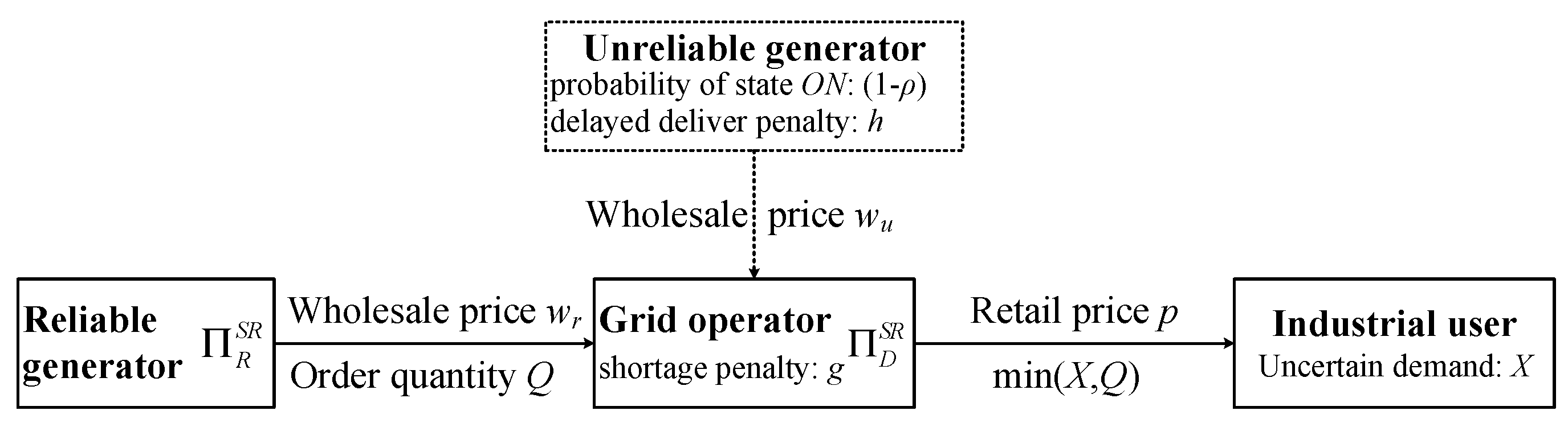
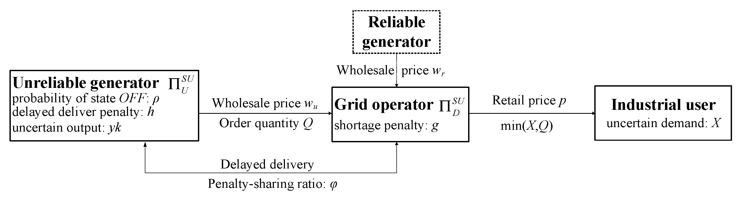
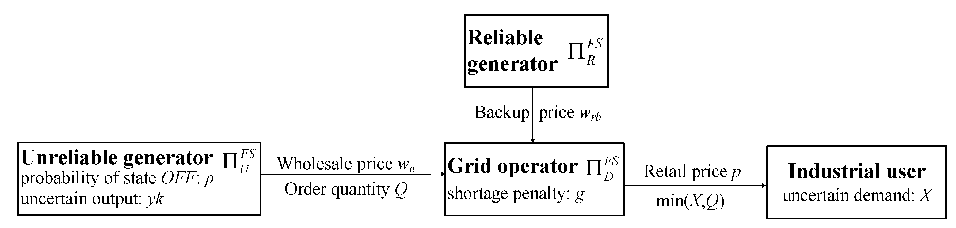
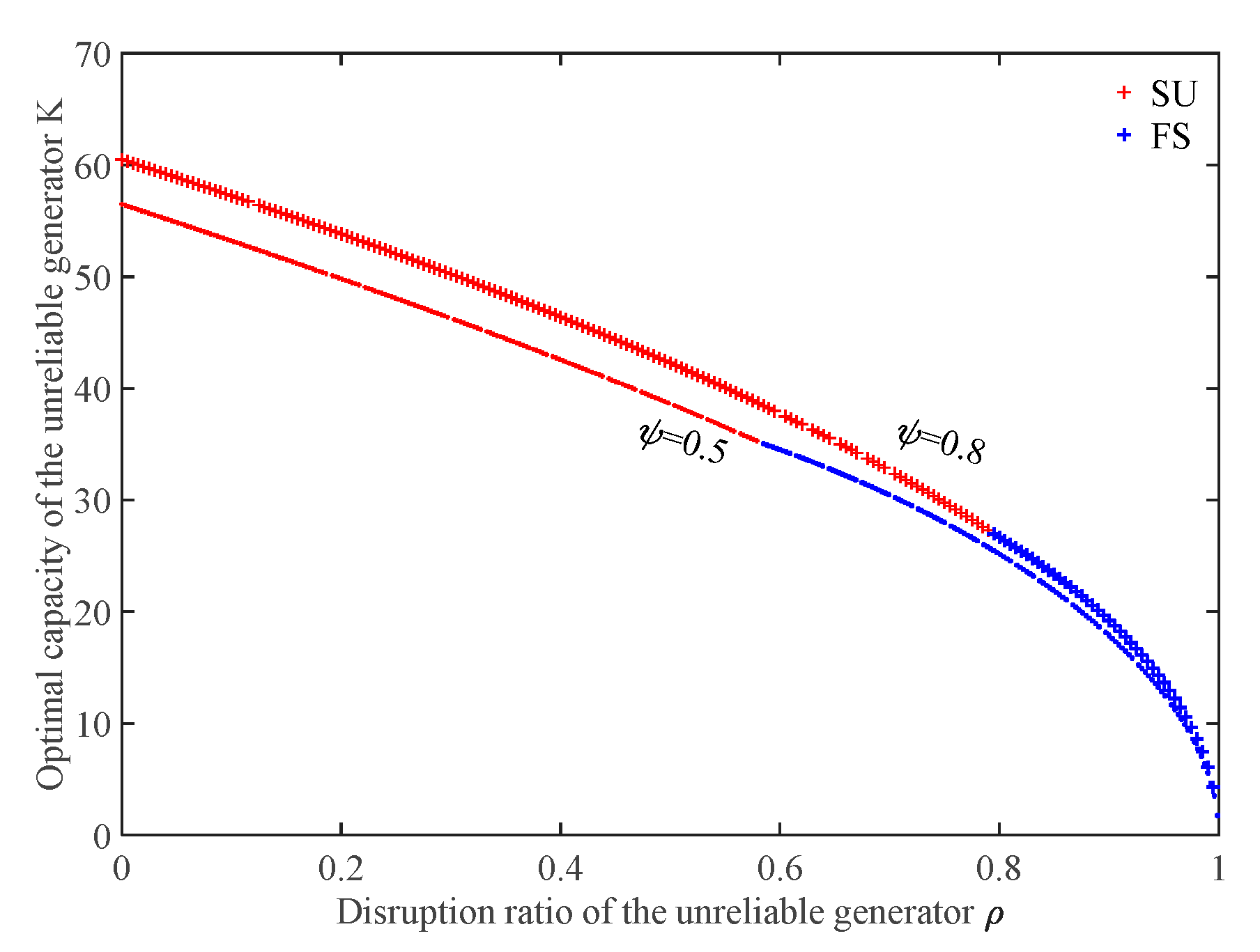
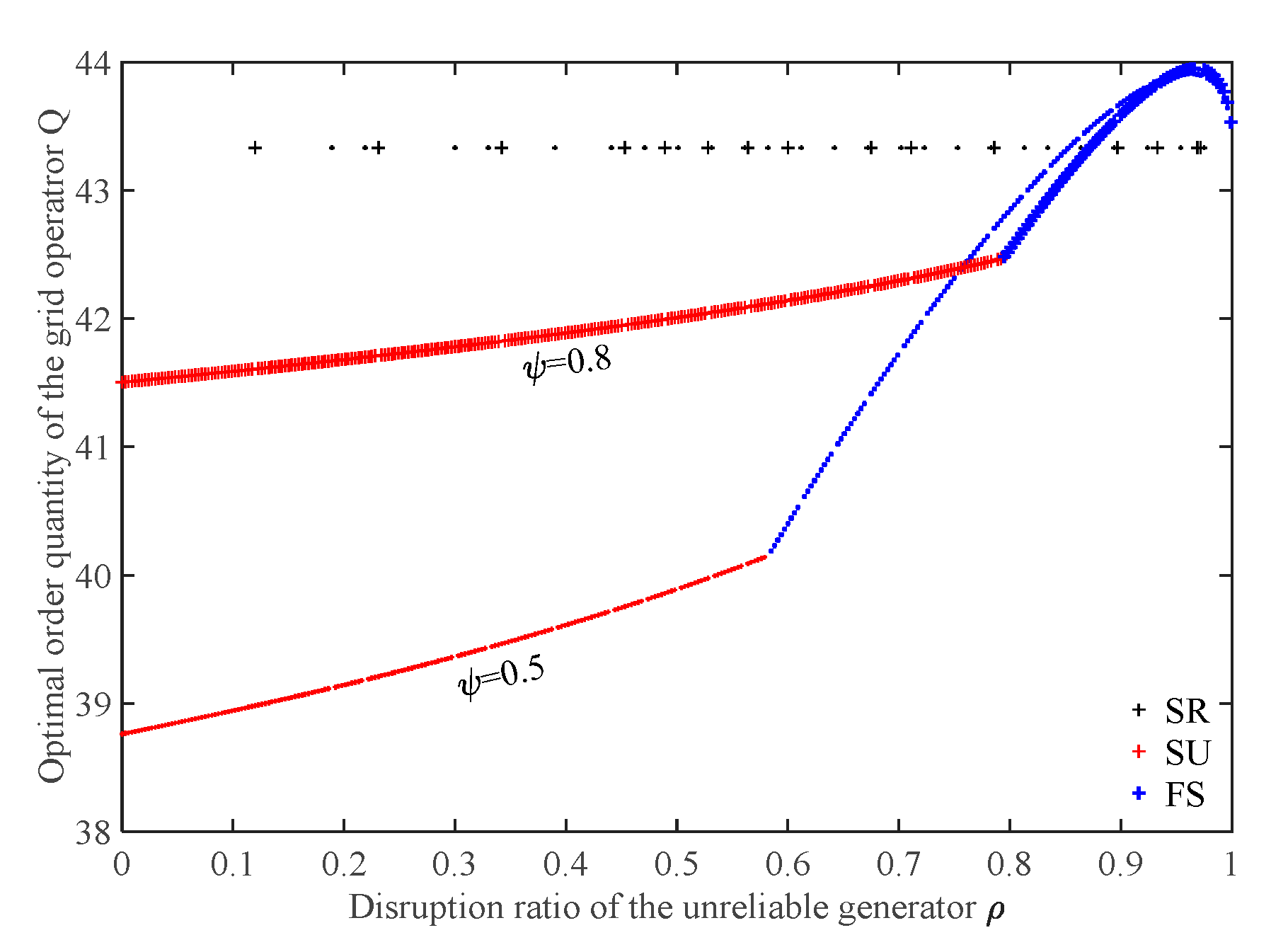
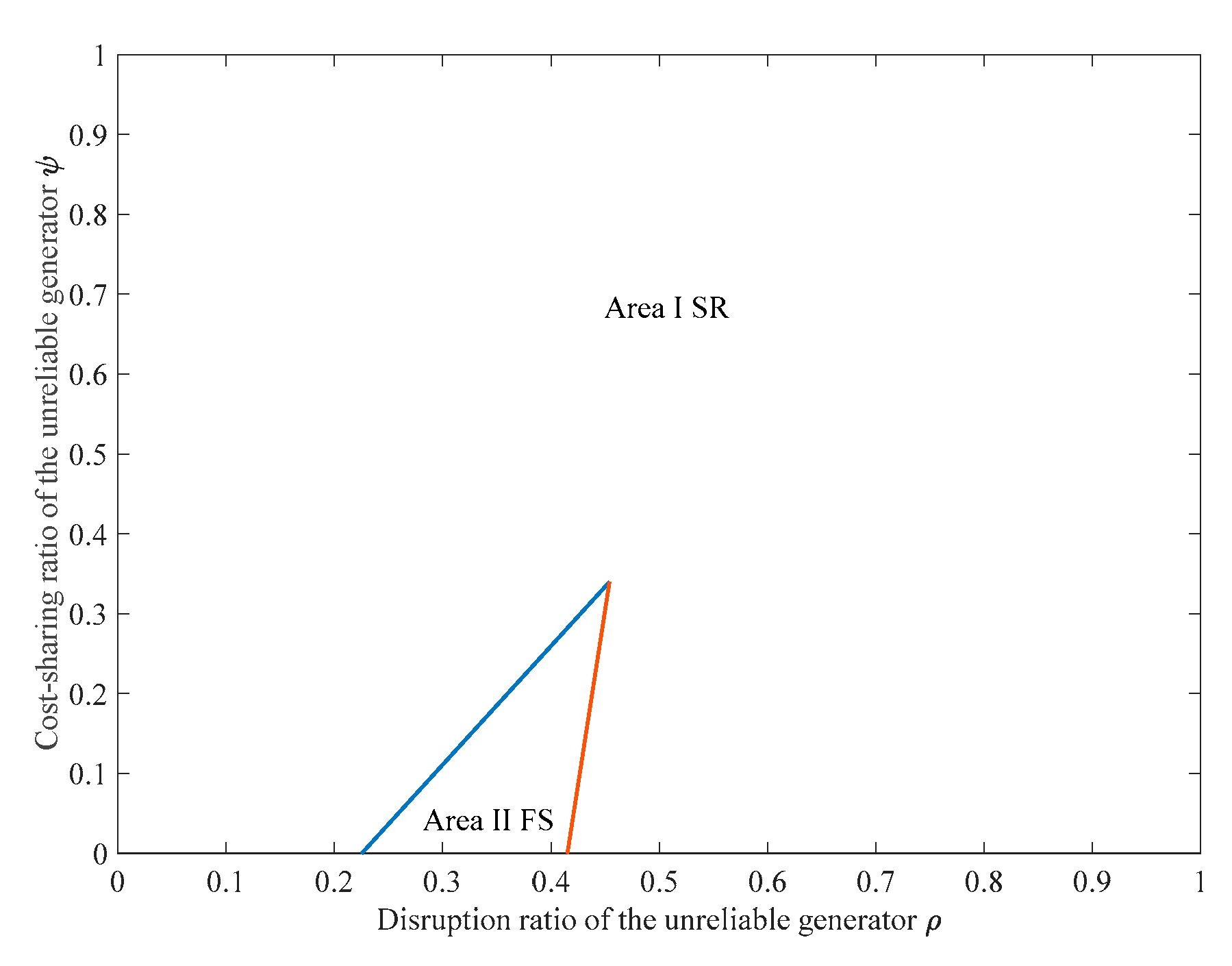
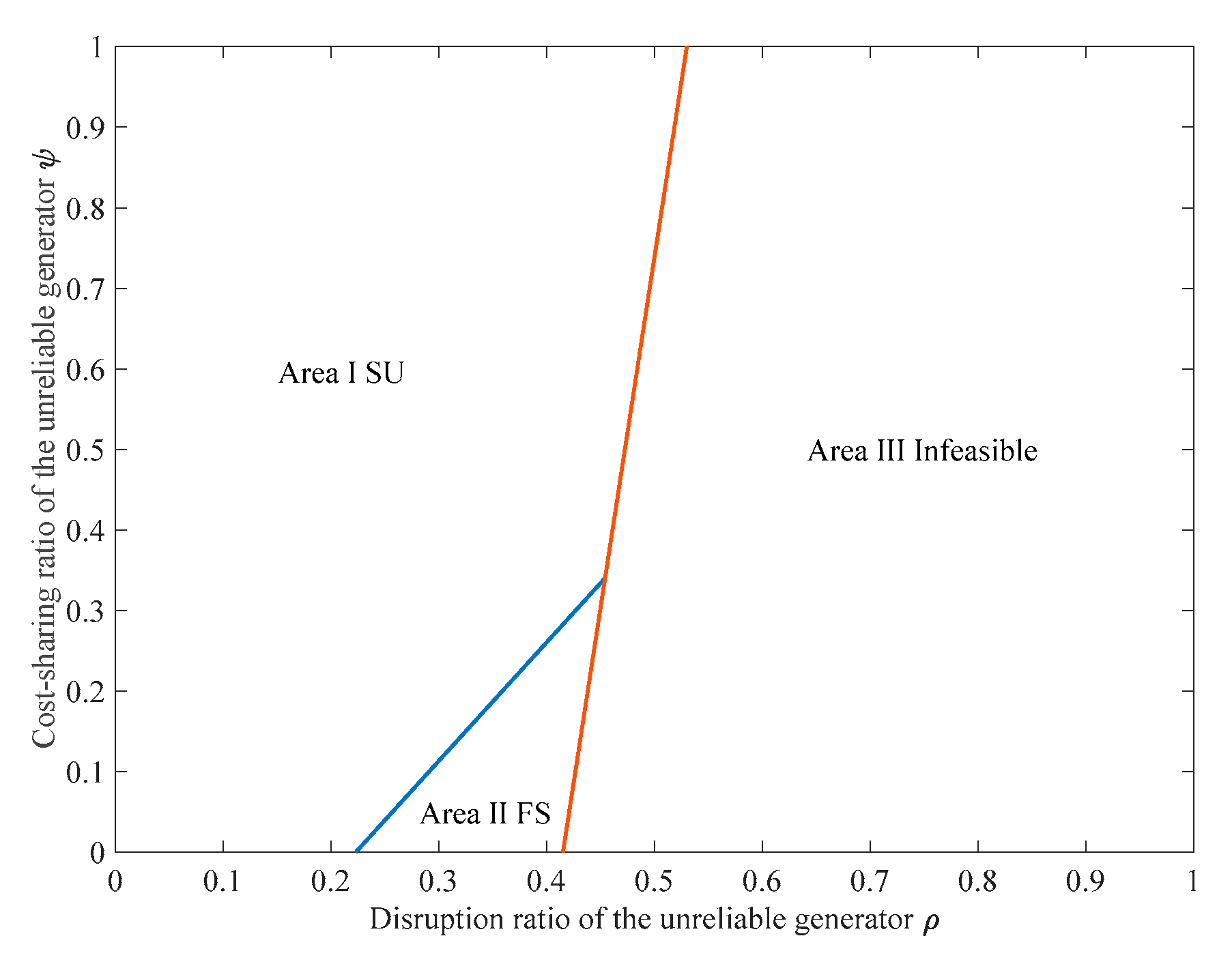
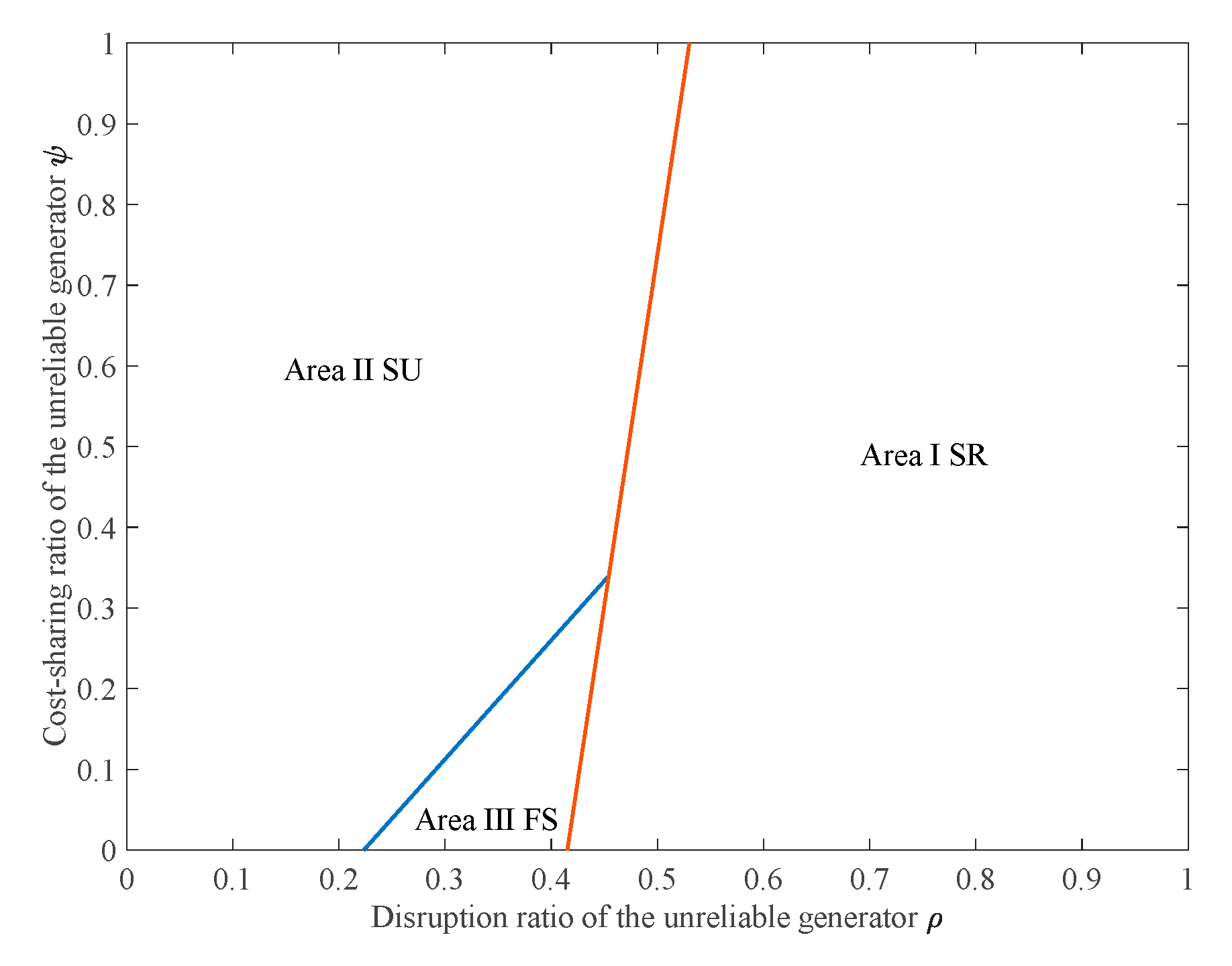
Table 1.
Notations.
| Symbol | Meaning |
|---|---|
| Generation cost of unreliable generator | |
| Generation cost of reliable generator | |
| Wholesale price of unreliable generator | |
| Wholesale price of reliable generator for regular orders | |
| Unit stock-out/shortage cost of the grid operator | |
| Penalty cost sharing ratio of unreliable generator | |
| Wholesale price of reliable generator for backup orders | |
| Selling price of grid operator | |
| Steady-state probability that the unreliable generator is ON, | |
| Steady-state probability that the unreliable generator is | |
| Investment in generation capacity of the unreliable generator | |
| The output intensity of regular capacity follows a cumulative distribution function is , and its probability density function is with mean , | |
| Orders of the grid operator | |
| The market demand follows a of , and its is with mean |
Table 2.
Notations.
| Mode | Symbol | Optimal Value |
|---|---|---|
| SR | ||
| SU | ||
| FS | ||
Table 3.
Parameter values in numerical study.
| Parameter | Values | Parameter | Values |
|---|---|---|---|
| 0.1 | 20% | ||
| 0.1 | 80% | ||
| 0.05 | 0~100 | ||
| 0.2 | 0~1 | ||
| 0.7 |
© 2019 by the authors. Licensee MDPI, Basel, Switzerland. This article is an open access article distributed under the terms and conditions of the Creative Commons Attribution (CC BY) license (http://creativecommons.org/licenses/by/4.0/).
Share and Cite
MDPI and ACS Style
Xie, J.; Wei, L.; Zhang, W.; Xia, Y.; Li, J. A Responsive Pricing Grid Operator Sourcing from Competing Generators under Uncertain Supply and Demand. Sustainability 2019, 11, 4061. https://0-doi-org.brum.beds.ac.uk/10.3390/su11154061
AMA Style
Xie J, Wei L, Zhang W, Xia Y, Li J. A Responsive Pricing Grid Operator Sourcing from Competing Generators under Uncertain Supply and Demand. Sustainability. 2019; 11(15):4061. https://0-doi-org.brum.beds.ac.uk/10.3390/su11154061
Chicago/Turabian StyleXie, Jiaping, Lihong Wei, Weisi Zhang, Yu Xia, and Jing Li. 2019. "A Responsive Pricing Grid Operator Sourcing from Competing Generators under Uncertain Supply and Demand" Sustainability 11, no. 15: 4061. https://0-doi-org.brum.beds.ac.uk/10.3390/su11154061
Note that from the first issue of 2016, this journal uses article numbers instead of page numbers. See further details here.