Evaluation of Empirical Reference Evapotranspiration Models Using Compromise Programming: A Case Study of Peninsular Malaysia

Abstract

Selection of appropriate empirical reference evapotranspiration (ET_o) estimation models is very important for the management of agriculture, water resources, and environment. Statistical metrics generally used for performance assessment of empirical ET_o models, on a station level, often give contradictory results, which make the ranking of methods a challenging task. Besides, the ranking of ET_o estimation methods for a given study area based on the rank at different stations is also a difficult task. Compromise programming and group decision-making methods have been proposed in this study for the ranking of 31 empirical ET_o models for Peninsular Malaysia based on four standard statistical metrics. The result revealed the Penman-Monteith as the most suitable method of estimation of ET_o, followed by radiation-based Priestley and Taylor and the mass transfer-based Dalton and Meyer methods. Among the temperature-based methods, Ivanov was found the best. The methodology suggested in this study can be adopted in any other region for an easy but robust evaluation of empirical ET_o models.

1. Introduction

Evapotranspiration (ET), the process of water release to the atmosphere, plays a crucial role in irrigation management [1], water balance estimation [2], surface runoff estimation [3], groundwater level prediction [4], water stress assessment [5], reservoir management [6], daily flux modelling [7], and climate change impact assessment [8]. It determines the crop irrigation requirement and thus, irrigation management, the introduction of new crop, or crop scheduling to adapt to climate change [9,10,11]. It is a major component that defines surface runoff and therefore, important for designing drainage and hydraulic structure [12,13]. In addition, it is the major component that determines the ecological or environmental water demand and thus, assessment of environmental sustainability or ecological balance [14]. It provides an assessment of water release from surface water bodies and reservoirs to the atmosphere and therefore, operation and management of water resources [15,16]. Hence, ET is considered as a vital component for any hydrological and climatic study [17]. Atmospheric water is an important driving factor of precipitation [18]. It has a significant effect on the retention of solar radiation and thus, controlling the air temperature of a region [19]. Therefore, the importance of the assessment of ET becomes more crucial in the context of climate change.

A most accepted method of ET estimation is to measure the reference evapotranspiration (ET_o) [20]. In-situ measurement of ET_o is expensive and time-consuming, and subject to significant uncertainties. Because of the limitation of in-situ measurements of ET_o, many empirical models have been developed to estimate ET_o in the last 70 years, since the introduction of the Thornthwaite method in 1944 [21]. The ET_o depends on atmospheric energy balance and release of water to the atmosphere from vegetation [22,23]. Therefore, the ET_o estimation methods are categorized according to the meteorological parameters they use. The ET_o method has been divided into different categories in different studies. Most widely, it is classified into four groups: (i) Water balance/mass transfer; (ii) radiation; (iii) temperature; and (iv) combination of the aforementioned. Each method has its own perspectives, concepts, and often developed for a particular climatic region. Few of them are developed through modification of other established methods. However, the main challenge in the estimation of ET_o is the skill of the method used [15,24]. Most of the ET estimation methods are developed for a particular region with a specific viewpoint, and therefore, they are often found inefficient in estimating ET_o in other climatic zones. However, some methods are developed without focusing on any climatic region and have been found applicable over a wide range of climate. The major challenge arises in the selection of the best model for an area with the least error compared to in-situ measurements.

ET is a crucial element in defining the water budget and physical processes in tropics. The condensation of the vast volume of water vapor in the tropical region leads to the release of latent heat energy to the atmosphere, which is very important for climatology in the region. Tropical regions, particularly the Southeast Asian tropical region, are rich in biodiversity. This rich biodiversity is promoted by high rainfall and high ET, among other factors. Changes in ET can have a severe impact on tropical biodiversity, and therefore, monitoring of ET is very important for the region. It is particularly crucial for Peninsular Malaysia where about 60% of its land is covered with forest with dense biodiversity.

A large number of studies have been conducted to select the most suitable ET_o model in different parts of the globe [15,20,25,26,27,28], including Peninsular Malaysia [13,29,30,31,32]. Ali et al. [30] and Ali et al. [31] found a strong agreement of the monthly average of class A pan evaporation with the FAO Penman-Monteith [33] estimation for the Muda irrigation project, the largest paddy field in Malaysia, in the north of the Peninsula. Tukimat et al. [13] compared a number of temperature- and radiation-based methods with the FAO Penman-Monteith model to estimate ET_o in the Muda irrigation project, and found that the radiation-based models give better estimates of ET_o. Lee et al. [29] compared the pan evaporation with the estimates of eight empirical models and found a good agreement between pan evaporation estimates of ET_o with the estimates of the FAO Penman-Monteith and FAO Blaney-Criddle [34] models in the west coast of the Peninsular. Muniandy et al. [32] compared the pan evaporation estimates with 26 empirical model estimations at a station located in the south of the Peninsular, and reported that the mass transfer-based Penman model can provide better estimates of ET_o compared to other methods.

Different statistics have been used in previous studies for the assessment of the performance of ET_o, which include root mean square error (RMSE), mean absolute error (MAE), Nash-Sutcliff efficiency (NSE), bias ratio, etc. Selection of ET_o method based on a single statistic like RMSE or NSE is questionable, as these statistics can be used for the estimation of a particular property only. For example, RMSE provides a measure of the mean distance between two time series, while correlation provides how two time series follow each other in their variation. The correlation coefficient (R²) can be excellent even if the distance between the two series is high, while RMSE can be much less even if one time series fails to follow the variation of another series. Thus, a number of statistical metrics are generally used for the assessment of the performance of different ET_o methods [13,15,25,26,27,28,29]. However, the major problem with using a number of statistical metrics is that different metrics often provide contradictory results [35,36,37]. For example, a model may show good agreement in terms of RMSE, but a worse measure in terms of R². Thus, it often becomes challenging to make a decision based on different statistics.

Compromise programming (CP) [38] can be used to find the most suitable solution through judicious compromising of different objectives, among which many may be conflicting. CP attempts to identify a solution where all the considered objectives achieve the most suitable value [39,40]. CP has been found more efficient compared to conventional multi-criteria decision analysis (MCDA) methods in finding the most suitable solution [38,40,41,42,43,44].

The ranking of the ET_o estimation method at a single station based on the ability to replicate the observed ET can be done using CP and a matrix of statistical indices. However, it is often required to suggest the best ET_o model for a region based on the performance at different stations over the region. Ranking of ET_o based on the performance at multiple stations becomes challenging, as different ET_o models often show different ranks at different stations. Group decision making (GDM) can be employed for such cases where the ET_o model is given a position based on the frequency of the rank obtained at different stations.

The objective of the present study is to use CP for the ranking of empirical ET_o models for Peninsular Malaysia. Four statistical metrics were used for the assessment of the performance of 31 ET_o models at 10 locations distributed over the Peninsula. CP was used for the ranking the empirical models at each of the 10 stations. Finally, an information aggregation approach was used for the ranking of the empirical models for the entire Peninsular Malaysia based on the results obtained at the different stations. This is the first approach of the ranking of empirical ET_o models based on CP and the information aggregation approach. The method proposed in this study can be used for the ranking of empirical models in a prudent way.

2. Study Area and Data

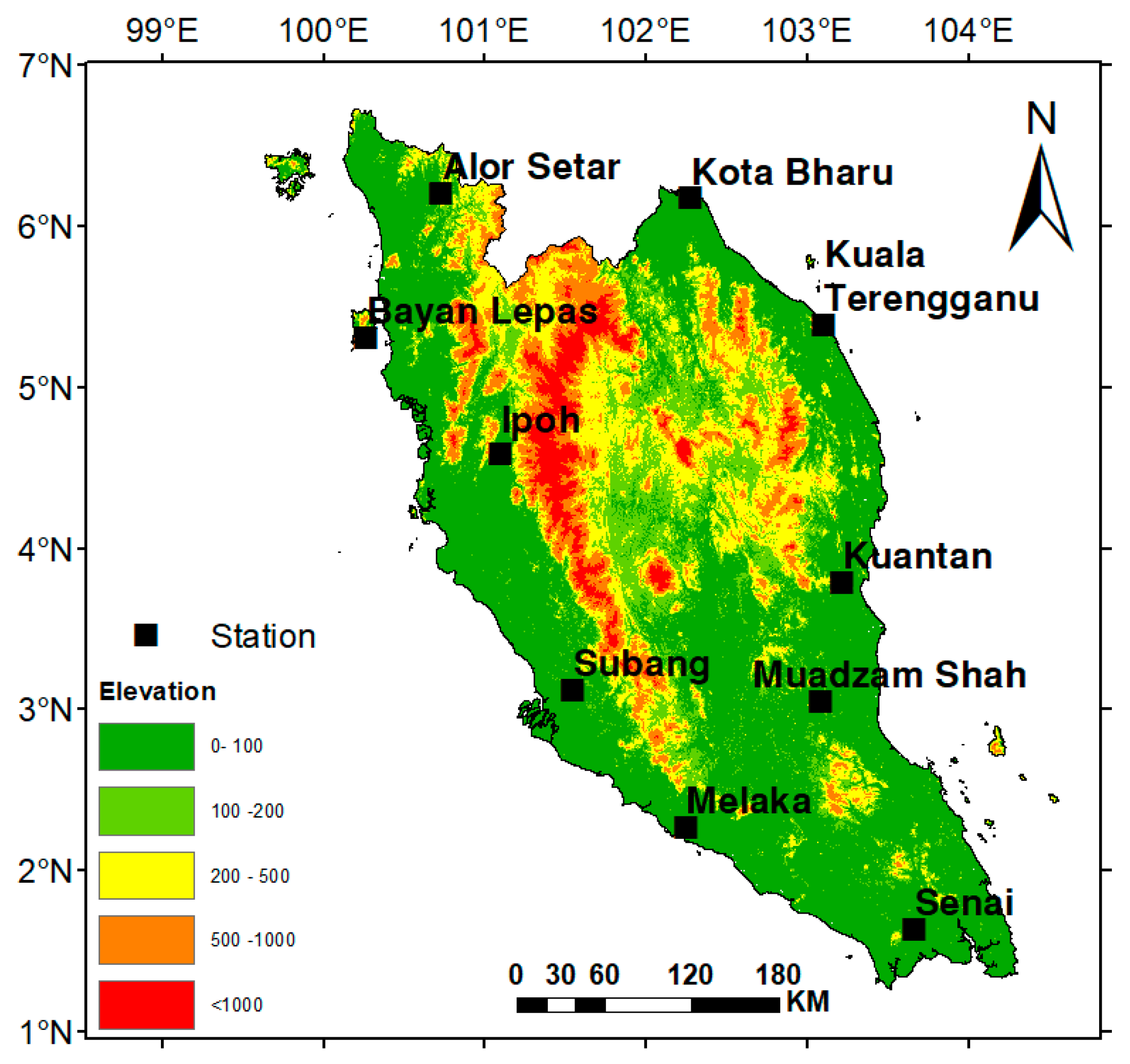
2.1. Geography and Climate of Peninsular Malaysia

Situated along the tropics, Peninsular Malaysia covers an area of 130,598 km² (Figure 1). Undulating mountains in the middle and relative flat coast on all the three sides (east, west, and south) are the major topographic features of the peninsula. About 60% of the land is covered by forest. The year-round rainfall, high uniform temperature, and high humidity are the major characteristics of the climate of Peninsular Malaysia. The climate is more or less homogeneous throughout the Peninsula [45,46]. Due to its geographical location, the weather in the region is influenced by both the northeast and the southwest monsoon, and thus experiences a significant amount of rainfall even in the driest month. The annual average rainfall in Peninsular Malaysia varies between 1950 and 4000 mm [47]. The number of rainfall days ranges between 150 and 200. Weather is always hot due to its location in the tropics, and humid due to high rainfall. The mean temperature in the peninsula varies between 23 °C in the central highlands and 32 °C in the coastal region [46,48]. Seasonal variation of mean temperature is always less than 2.0 °C from the mean temperature of 27 °C. Being located in the equator, the study area receives long daylight hours (about 12 h) throughout the year and, thus, sufficient solar radiation. The wind in peninsular Malaysia is mostly light (0.9 to 2.3 m/s). Sunshine hours and temperature have an important role in ET_o in the study area. The ET_o is lower in the rainy season due to lower sunshine hours. Furthermore, it is lower in central mountainous areas (2.5 mm/day) due to relatively higher humidity compared to the coastal region (4–5 mm/day), where the humidity is less.

2.2. Data and Sources of Information

The observed daily meteorological data of temperature (mean, maximum, and minimum), relative humidity, solar radiation, wind speed, and pan evaporation from 10 meteorological stations fairly distributed over Peninsular Malaysia were collected from the Malaysian Meteorological Department. The locations of the meteorological stations are shown in Figure 1. The summary of the different climatic variables used in the present study is given in

Table 1. Descriptive statistics of the meteorological stations used in the present study.

Station Name	Station No	Elev. (m)	Time Period	Tmax (°C)	Tmin (°C)	Tmean (°C)	RH (%)	u (m/s)	Rs (MJ/m2)	ETpan (mm/day)
Alor Star	48603	3.9	1985–2014	32.4	23.4	27.1	81.2	1.5	18.5	3.4
Bayan Lepas	48601	2.5	1985–2014	31.4	23.9	27.2	80.4	1.8	17.9	2.9
Kota Bharu	48615	4.4	2000–2014	31.2	23.5	26.9	80.6	2.3	18.9	3.2
Ipoh	48625	40.1	1985–2014	33.0	23.3	27.0	81.3	1.4	17.7	3.1
Kuala Terengganu	48618	5.2	2005–2008	31.4	23.8	27.0	82.4	1.9	17.5	3.3
Subang	48647	16.6	1985–2014	32.4	23.2	26.9	79.6	1.5	16.5	3.2
Kuantan	48657	15.2	1999–2014	31.7	22.9	26.2	84.1	1.7	17.0	2.9
Muadzam Shah	48649	33.3	1985–2014	32.1	22.7	26.3	84.7	0.9	16.3	2.5
Melaka	48665	9.0	1999–2010	31.9	23.2	26.8	80.1	1.7	17.0	3.3
Senai	48679	37.8	1985–2010	31.8	22.5	26.0	85.7	1.4	15.1	2.7

RH is the relative humidity; u is the wind speed; R_s is the solar radiation; and ETpan is the pan evaporation.

.

Pan evaporation is an indirect and less expensive method of estimation of ET and therefore, it is most widely used for estimation of ET. The pan evaporation data is multiplied by the pan coefficient to get the ET_o. The pan coefficient value varies between 0.35 and 0.85, depending on the nature of the evaporating surfaces (land use), altitude, average humidity, and average wind speed of the site [49]. Considering the existing setup, the Department of Irrigation and Drainage of Malaysia [50] suggested a pan coefficient of 0.75 for the estimation of ET_o from pan evaporation in Malaysia. Therefore, the observed ET_o was calculated by multiplying the pan evaporation data by the pan coefficient of 0.75.

3. Methodology

The performance of different empirical ET_o models was assessed and ranked by comparing their estimations with the in-situ data. The methodology adopted in this study is summarized below.

• ET_o was estimated by the empirical models using the metrological variables.
• Four statistical metrics were used to estimate the capability of different empirical ET_o models to estimate different properties of observed ET_o at each station.
• CP was used to integrate the results of statistical metrics and rank the ET_o models at each station.
• GDM, an information accumulation method, was deployed to rank the empirical models for the entire Peninsula.

3.1. Empirical ET_o Models

In this study, 31 empirical ET_o models were evaluated by comparing their estimates with the pan evaporation data. They were selected based on their applicability worldwide and the availability of required input data. The empirical models were classified into four groups based on the input parameters. Out of 31 models, 10 are temperature-based, 10 are radiation-based, 10 are mass transfer-based models, and one is a combination model. The ET_o was calculated using the meteorological input at each station location without any calibration.

Table 2. List of the empirical reference evapotranspiration (ET_o) models evaluated in this study, along with their input parameters and equations. They are classed into four groups: Temperature-based, radiation-based, mass transfer-based, and combination.

No	Model	Input Parameter	Equation
Temperature-based
1	Ivanov [51]	Tmean, RH	ETo = $0.00006{\left(25+T_{mean}\right)}^2\left(100-RH\right)$
2	Hamon [52]	Tmean	ETo = $0.1651L_d$ RHOSAT × KPEC RHOSAT = $\frac{216.7\mathrm{ESAT}}{T_{mean}+273.3}$ ESAT = $6.108\exp \left(\frac{17.269\times T_{mean}}{T_{mean}+273.3}\right)$
3	Papadakis [53]	Tmean, RH	ETo = $2.5\left(e_{ma}-e_a\right)$
4	Schendel [54]	Tmean, RH	ETo = $16\left(\frac{T_{mean}}{\mathrm{RH}}\right)$
5	FAO Blaney-Criddle [34]	Tmean	ETo = $p\left(0.46T_{mean}+8.13\right)$
6	Linacre [55]	Tmean	ETo = $\frac{\frac{700\left(T_{mean}\pm 0.006z\right)}{100-L}+15\left(T_{mean}-T_d\right)}{80-T_{mean}}$
7	Kharrufa [56]	Tmean	ETo = $0.34p{T}_{mean}{}^{1.30}$
8	Hargreaves et al. [57]	Tmean, Tmin, Tmax, Ra	ETo = $\left(0.0023\frac{R_a}{2.45}\right)T{D}^{0.5}\left(T_{mean}+17.8\right)$
9	Trajkovic [58]	Tmean, Tmin, Tmax, Ra	ETo = $\left(0.0023R_a\right)T{D}^{0.424}\left(T_{mean}+17.8\right)$
10	Ravazzani et al. [59]	Tmean, Tmin, Tmax, Ra	ETo = $\left(0.817+0.00022z\right)\left(0.0023R_a\right)\left(T{D}^{0.5}\right)\left(T_{mean}+17.8\right)$
Radiation-based
11	Makkink [60]	Tmean, Rs	ETo = $0.61\left(\frac{\mathsf{\Delta }}{\mathsf{\Delta }+\gamma }\right)\frac{R_s}{58.5}-0.12$
12	Turc [61]	Tmean, Rs, RH	ETo = $0.013\left(\frac{T_{mean}}{T_{mean}+15}\right)\left(R_s+50\right)$
13	Jensen et al. [62]	Tmean, Rs	ETo = $\left(\frac{R_s}{\lambda }\right)\left(0.025T_{mean}+0.08\right)$
14	Priestley et al. [63]	Tmean, Rs, RH	ETo = $\alpha \left(\frac{\mathsf{\Delta }}{\mathsf{\Delta }+\gamma }\right)\frac{R_n}{\lambda }$
15	McGuinness et al. [64]	Tmean, Rs	ETo = $\left(0.0082T_{mean}-0.19\right)\frac{R_s}{1500}\left(2.54\right)$
16	Caprio [65]	Tmean, Rs	ETo = $\left(\frac{6.1}{{10}^6}\right)R_s\left(1.8T_{mean}+1.0\right)$
17	Jones et al. [66]	Tmin, Tmax, Rs	ETo = ${\alpha }_1\left(3.87\times {10}^{-3}\right)\left(R_s\left(0.6T_{max}+0.4T_{min}+29\right)\right)$
18	Abtew [67]	Tmean, Rs	ETo = $0.53\left(\frac{R_s}{\lambda }\right)$
19	Irmak et al. [12] -Rs	Tmean, Rs	ETo = $-0.611+0.149R_s+0.079T_{mean}$
20	Irmak et al. [12] -Rn	Tmean, Rs, RH	ETo = $0.489+0.289R_n+0.023T_{mean}$
Mass transfer-based
21	Dalton [68]	Tmean, RH, u	ETo = $\left(0.3648+0.07223\left(u\right)\right)\left(e_s-e_a\right)$
22	Trabert [69]	Tmean, RH, u	ETo = $\left(0.3075\right)\sqrt{u}\left(e_s-e_a\right)$
23	Meyer [70]	Tmean, RH, u	ETo = $\left(0.375+0.05026\left(u\right)\right)\left(e_s-e_a\right)$
24	Rohwer [71]	Tmean, RH, u	ETo = $\left(3.3+0.891\left(u\right)\right)\left(e_s-e_a\right)$
25	Penman [72]	Tmean, RH, u	ETo = $\left(2.625+0.000479/u\right)\left(e_s-e_a\right)$
26	Albrecht [73]	Tmean, RH, u	ETo = $\left(0.1005+0.297\left(u\right)\right)\left(e_s-e_a\right)$
27	Brockamp et al. [74]	Tmean, RH, u	ETo = $0.543\left(u^{0.456}\right)\left(e_s-e_a\right)$
28	WMO [75]	Tmean, RH, u	ETo = $\left(0.1298+0.0934\left(u\right)\right)\left(e_s-e_a\right)$
29	Mahringer [76]	Tmean, RH, u	ETo = $\left(0.15072\right)\sqrt{3.6u}\left(e_s-e_a\right)$
30	Szasz [77]	Tmean, RH, u	ETo = $0.00536{\left(T_{mean}+21\right)}^2{\left(1+RH\right)}^{2/3}f\left(u\right)$ $f\left(u\right)=\left(0.0519u\right)+0.905$
Combination-based
31	FAO Penman-Monteith [33]	Tmean, Rs, RH, u, es	ETo = $\frac{0.408\left(R_n-G\right)+\gamma \frac{900}{T_{mean}+273}u\left(e_s-e_a\right)}{\mathsf{\Delta }+\gamma \left(1+0.34u\right)}$

lists the input parameters and the equation of each of the 31 empirical models.

ET_o is the evapotranspiration in mm/day in all equations except the Ritchie and McGuinness and Bordne models, where ET_o is in cm/day. R_n is the net radiation (MJ/m²/day). G is the soil heat flux (MJ/m²/day). R_a is the extraterrestrial radiation (MJ/m²/day). Γ is the psychrometric constant (kPa/°C). e_s is the saturation vapor pressure (hPa). e_a is the actual vapor pressure (hPa). e_s and e_a are in hPa in all equations except the Papadakis, Rohwer, Penman, and FAO Penman-Monteith models, where e_s and e_a are in kPa. Δ is the slope of the saturation vapor pressure–temperature curve (kPa/°C). λ is the latent heat of evaporation (MJ/kg). T_mean is the average daily air temperature (°C). T_mean is in °C in all equations except the McGuinness and Bordne model, where T_mean is in °F. u is the mean daily wind speed at 2 m (m/s). f(u) is a function of wind speed. Z is the elevation (m). L is local latitude (degrees). T_d is the dew point temperature (°C). T_min is the minimum air temperature (°C). T_max is the maximum air temperature (°C). TD is the maximum and minimum temperature difference (°C). RH is the average relative humidity (%). Rs is the solar radiation. Rs is in MJ/m²/day in all equations except the Turc, Makkink, Ritchie and McGuinness, and Bordne models, where Rs is in Cal/m² day, and the Caprio model, where Rs is in kJ/m² day. e_ma is the saturation vapor pressure at the monthly mean daily maximum temperature (kPa). $p$ is the mean annual percentage of daytime hours for different latitudes that can be obtained from Doorenbos et al. [34]. $p$ is expressed as constant (0.274) in Muniandy et al. [32]. L_d is the daytime length in multiples of 12 h. RHOSAT is saturated vapor density (g/m³). ESAT is the saturated vapor pressure (mbar). KPEC is the calibration coefficient (1.2). α is a constant (1.26). α₁ is a constant (1.1).

3.2. Statistical Indices

Four statistical metrics were used to measure the capability of each empirical model in estimating the observed ET_o at each gauge location. They were the normalized root mean square error (NRMSE), percentage of bias (%BIAS), modified index of agreement (md), and Kling-Gupta efficiency (KGE). The NRMSE is a measure of accuracy as it calculates the magnitudes of the errors in modeled data [78]. The %BIAS quantifies the tendency of ET_o estimation by empirical models to under or over-estimate the observed data [36]. The md summarizes the additive and proportional differences in the observed and modeled ET_o means and variances. The KGE integrates linear correlation (r), bias ratio (β), and variability (γ) of observed and modeled data [35,79].

Table 3. The metric equations, range, and optimum value.

Metric Equation		Range	Optimum Value
$NRMSE=\frac{{\left[\frac{1}{n}{{\displaystyle \sum }}_{i=1}^n{\left(E{T}_0{}_{m,i}-E{T}_0{}_{obs,i}\right)}^2\right]}^{\raisebox{1ex}{$1$}\!\left/ \!\raisebox{-1ex}{$2$}\right.}}{\frac{1}{n}{{\displaystyle \sum }}_{i=1}^n\left(E{T}_0{}_{m,i}\right)}$	(1)	0 to +∞	0
$\%BIAS=100\times \left[\frac{{{\displaystyle \sum }}_{i=1}^n\left(E{T}_0{}_{m,i}-E{T}_0{}_{obs,i}\right)}{{{\displaystyle \sum }}_{i=1}^{n}E{T}_0{}_{m,i}}\right]$	(2)	−∞ to +∞	0
$md=1-\frac{{{\displaystyle \sum }}_{i=1}^n{\left(E{T}_0{}_{obs}-E{T}_0{}_m\right)}^j}{{{\displaystyle \sum }}_{i=1}^n{\left(\left|E{T}_0{}_m-\overline{E{T}_0{}_{obs}}\right|+\left|E{T}_0{}_{obs}-\overline{E{T}_0{}_{\mathrm{o}bs}}\right|\right)}^j}$	(3)	0 to 1	1
$KGE=1-\sqrt{{\left(r-1\right)}^2+{\left(\beta -1\right)}^2+{\left(\gamma -1\right)}^2}$	(4)	−∞ to 1	1

$E{T}_0{}_{m,i}$ and $E{T}_0{}_{obs,i}$ are the i-th modeled and observed ET₀ data; $n$ is the number of observations; j represents an arbitrary positive power; r is the Pearson correlation; β is the bias ratio; and γ represents the variability of observed and modeled data.

presents each metric equation, range, and optimum value.

3.3. Compromise Programming

Compromise programming (CP) was used to integrate the results of the statistical metrics described above to enable selection of the most accurate empirical ET_o model. CP ranks the empirical methods based on the distance of each method from an ideal value for the set [42,80]. The CP index (CPI) can be calculated as follows.

$$CPI={\left[{\displaystyle \sum }_{i=1}^n{\left|x_i-x_i^{*}\right|}^p\right]}^{1/p}$$

(5)

where i represents the result of a statistical metric; $x_i$ is the normalized value of metric i of the empirical model; and $x_i^{*}$ is the normalized ideal value of the metric i. The parameter p is used to measure the distance of a solution from an ideal point. The p can have a value between 1 and ∞. However, 1, 2, and ∞ are most commonly used in CP [81,82]. Therefore, these values are used in this study to estimate the CPI. The differences between the observed value of the metrics and $x_i^{*}$ are directly proportional to their magnitude when p = 1. The higher differences have greater influence in the case of p = 2. When p = ∞, the minimum values of the maximum differences are used for the estimation of the CPI. Details of the method can be found in [37,80].

In this study, we considered equal importance of all the ET_o estimation models and therefore, the weight parameter of the CP method proposed by Zeleny [38] is not considered. The CPI value ranges between zero and positive infinity, where zero is the most preferable value.

3.4. Ranking the Empirical ET_o Models

The ranking of empirical models in estimating observed ET_o from several stations was a challenging task. This was due to the fact that a model may show various degrees of accuracies at different locations. To overcome this challenge, information aggregation methods, such as mean ranking, majority of ranks, and frequency of occurrence, were useful [42,83]. They integrate information from different sources to help in the decision-making process [84]. In this study, empirical models were ranked using GDM. The ranking procedure is outlined below.

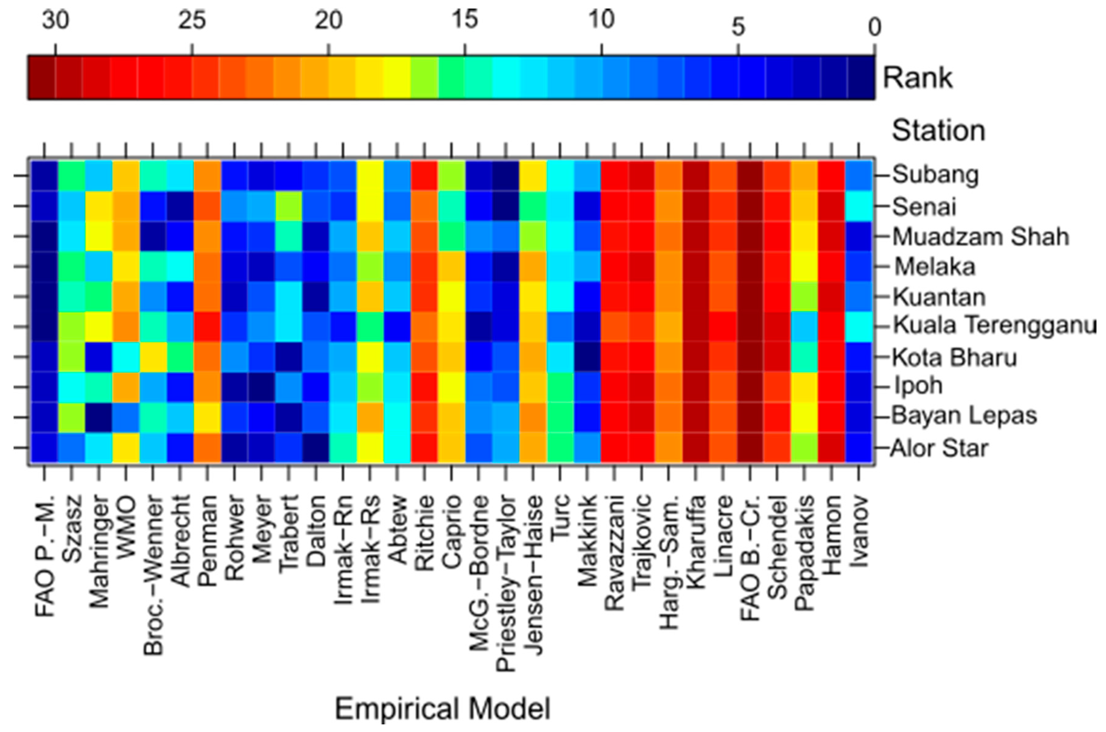
• The empirical models were ranked at station level using their CPI (from 1 to 31, the lowest CPI was ranked 1st).
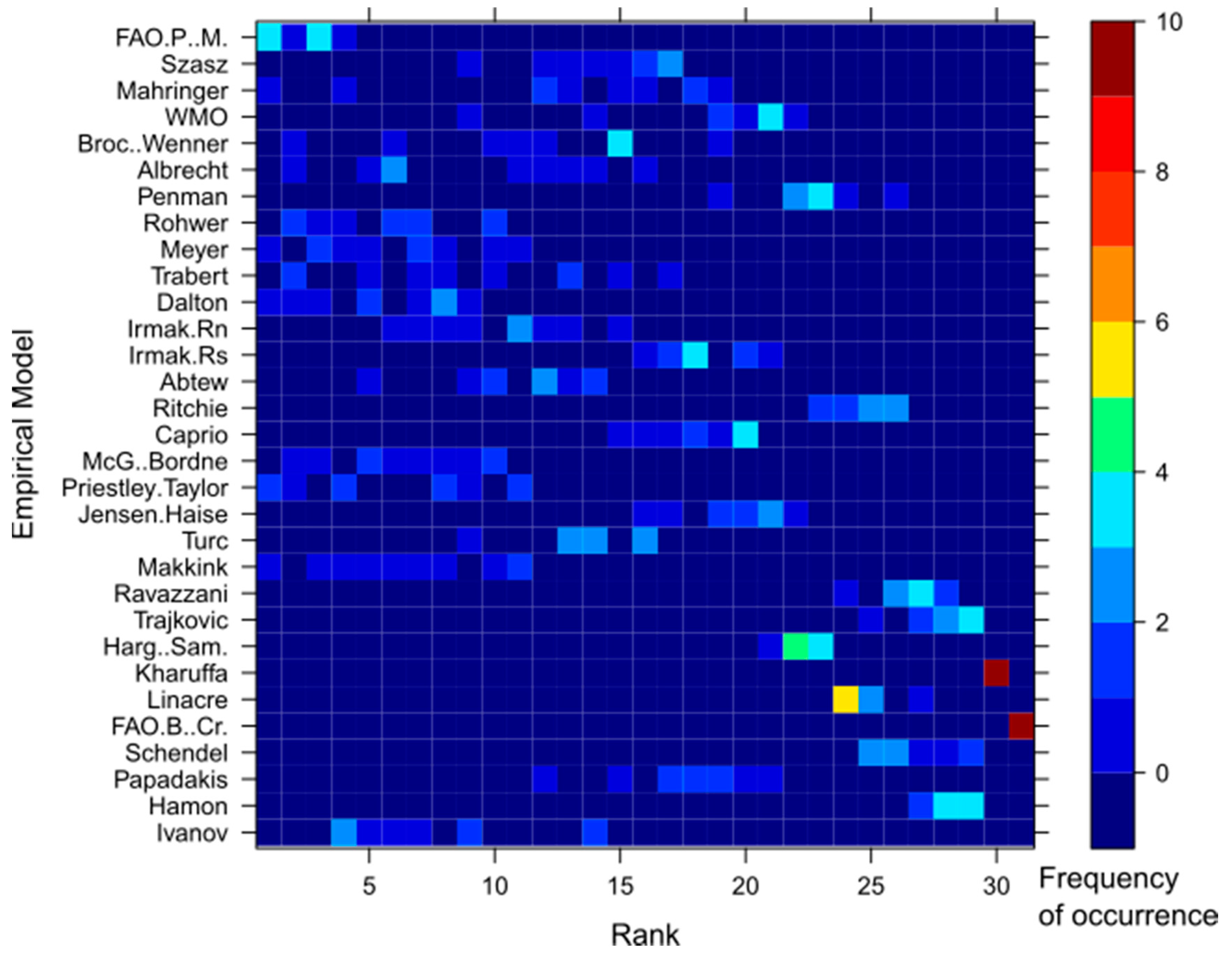
• The frequency of occurrence ($F$) of each model of getting a certain rank at all stations was calculated through a 31 × 31 matrix.
• The rank positions were given weight as the inverse of the rank $\left(w_r= ran{k}^{-1}\right)$.
• The frequency of occurrence of a model at a certain rank, obtained in Step 2, was multiplied by the weight of the rank, obtained in Step 3.
• The overall score of each ET_o model ($W_m$) was estimated by adding the output of Step 4 as presented in Equation (6).
• The empirical models were ranked according to the calculated overall weight, where the highest weighted model was ranked top (1st position).

$$W_m=F_1\left(w_{r1}\right)+F_2\left(w_{r2}\right)+F_3\left(w_{r3}\right)+.\dots +F_{31}\left(w_{r31}\right)$$

(6)

4. Results

The ET_o was estimated using all the 31 empirical models at each station, using the meteorological variables. Figure 2 shows heat-scatter plots of observed ET_o against each empirical model estimation of ET_o for all the stations. It can be seen from Figure 2a–t, all the temperature- and radiation-based models tend to overestimate the observed ET_o except for the Ivanov and Makkink model. The overestimation was generally lower by the radiation-based models (Figure 2k–t) than the temperate-based models, which indicates that the overestimation may be due to the exclusion of other factors influencing ET_o in the study area. The Ritchie model was found to heavily overestimate the observed ET_o, as seen in Figure 2q. Overall, the mass transfer-based models’ estimations (Figure 2u–ad) were found to be more aligned to the 1:1 diagonal line than the temperature- and radiation-based methods. The Penman, WMO, and Mahringer models underestimated the observations. The FAO Penman-Monteith model estimations of ET_o were aligned with the 1:1 line (Figure 2ae).

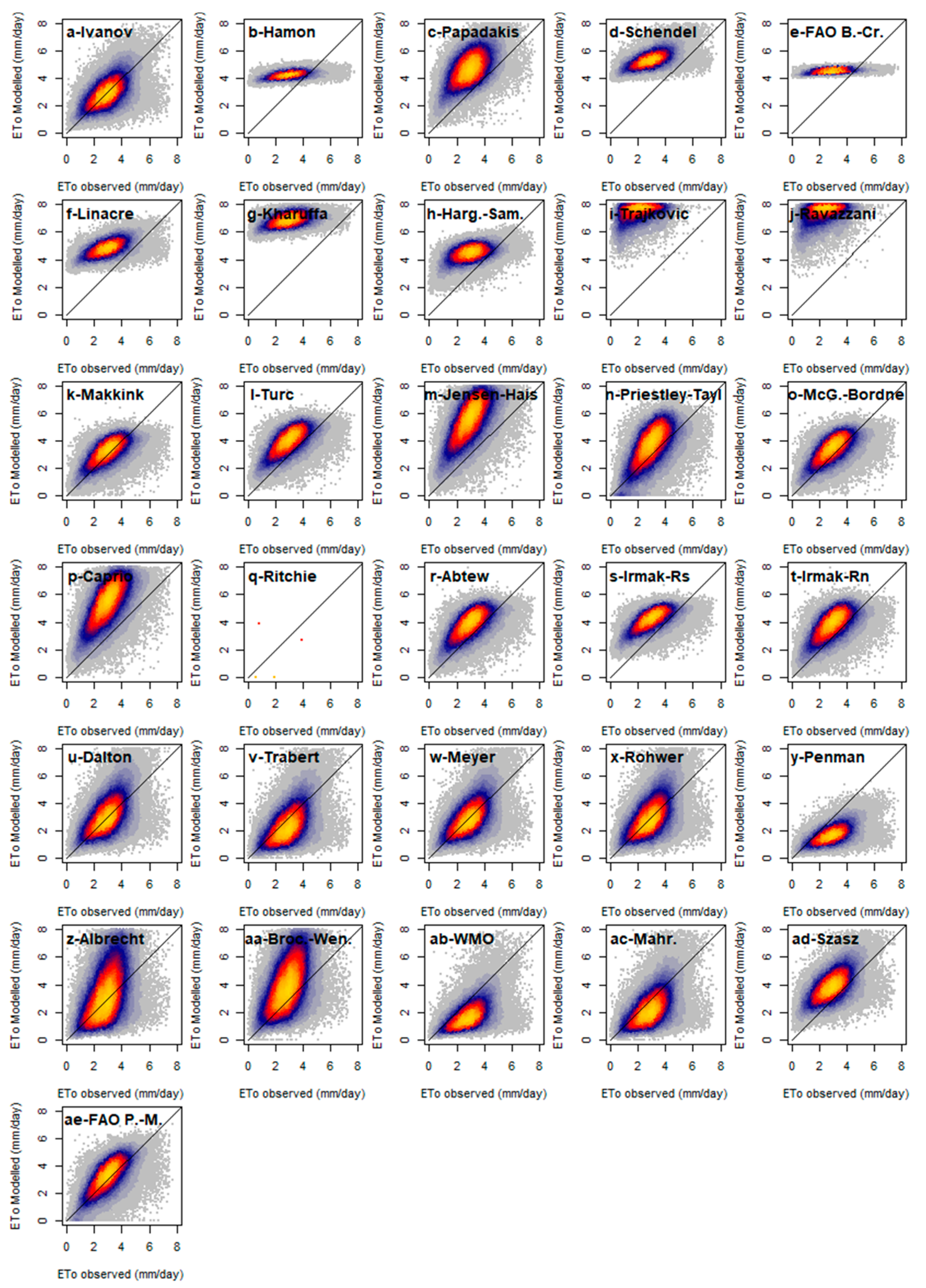
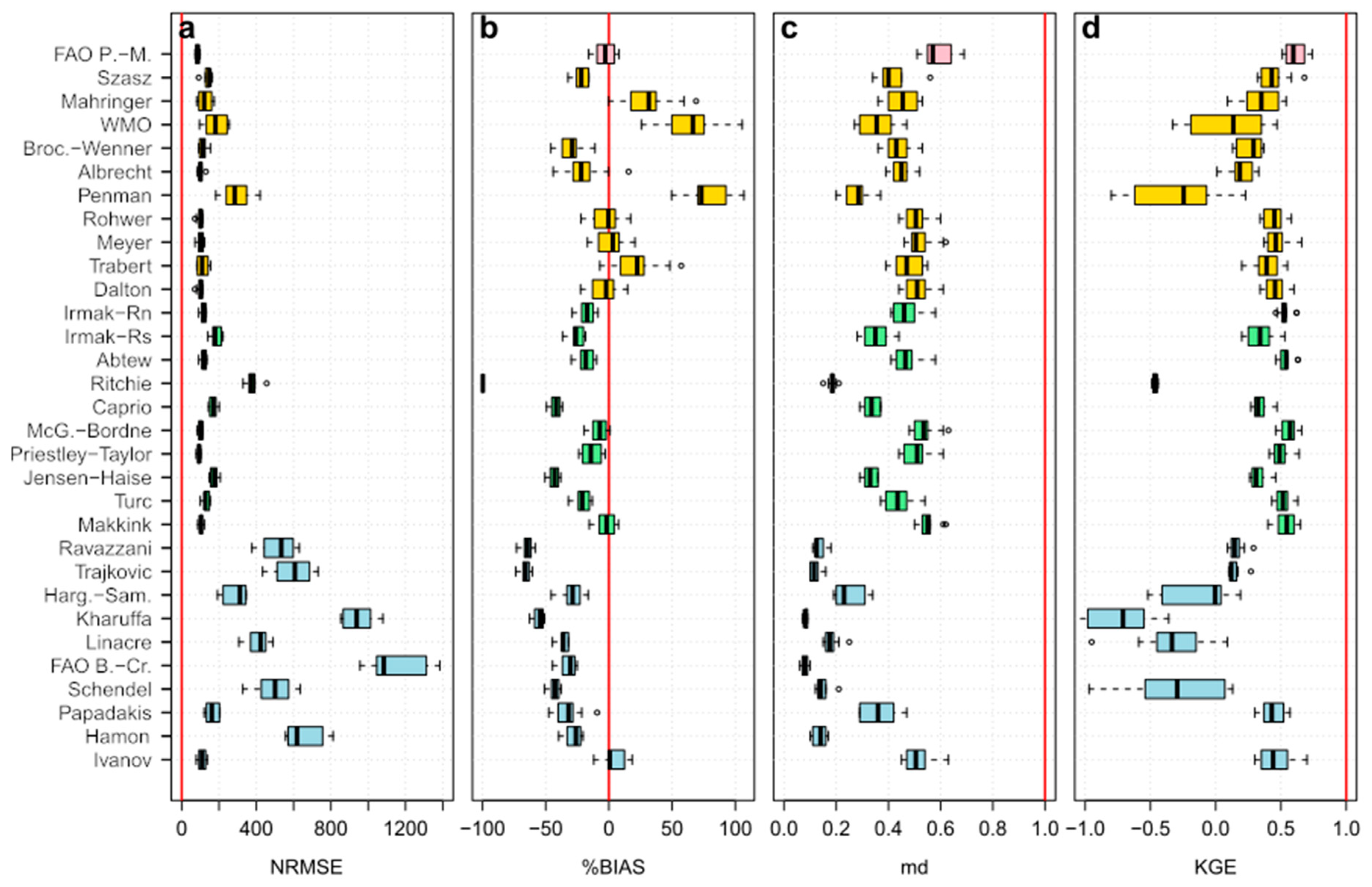
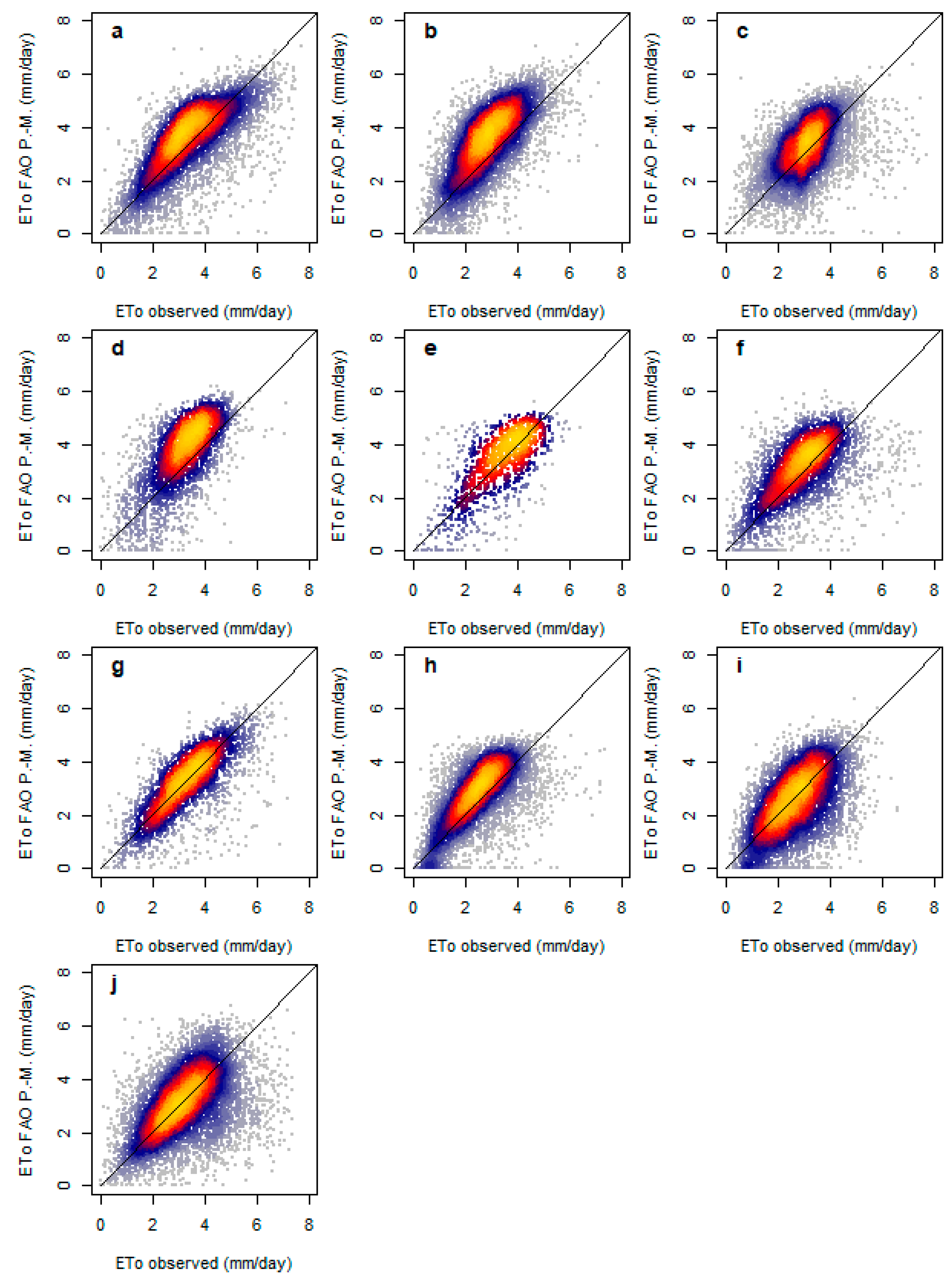
4.1. Evaluation Using Statistical Metrics

The statistical metrics obtained at all the 10 station locations by comparing the observed ET_o with the different empirical model estimations are presented as box plots in Figure 3. The blue, green, gold, and pink box plots represent the temperature-, radiation-, mass transfer-, and combination-based methods, respectively. The red vertical lines represent the optimum value of each metric. Overall, most of the temperature-based methods were found to be poor at estimating the ET_o. Among the temperature-based methods, the Ivanov model was found preferable, which had a median NRMSE of 108.8, median %BIAS of 0.70%, median md of 0.51, and median KGE of 0.44.

The performance of radiation-based methods was found superior to temperature-based models in estimating ET_o. The Makkink model was the best performing model among them, and the Ritchie was the worst. As shown in Figure 3, Makkink had the lowest median %BIAS (−1.80%), and highest median md (0.55). However, the Priestley and Taylor model had a slightly better median NRMSE (94.35) than Makkink (102.10). The McGuinness and Bordne model had a better median KGE (0.57) than Makkink (0.55).

Among the mass transfer-based models, the Rohwer and Meyer’s methods performed best. Rohwer had median NRMSE, %BIAS, md, and KGE of 104.25, −0.40%, 0.51, and 0.45, respectively. The Meyer model had median NRMSE, %BIAS, md, and KGE of 103.45, 3.10%, 0.51, and 0.45, respectively. The FAO Penman-Monteith had a median NRMSE of 85, %BIAS of −2.90%, md of 0.57, and KGE of 0.60.

The FAO Penman-Monteith model had the lowest NRMSE median, and the highest md and KGE medians. However, the Rohwer model had a lower %BIAS median than the FAO Penman-Monteith model. The Rowher, Meyer, and Makkink models had similar NRMSE, but Rowher had the lowest %BIAS, and Makkink had the highest md and KGE medians. Therefore, it is important to use CP to integrate the results of the statistical metrics to make a concrete evaluation decision.

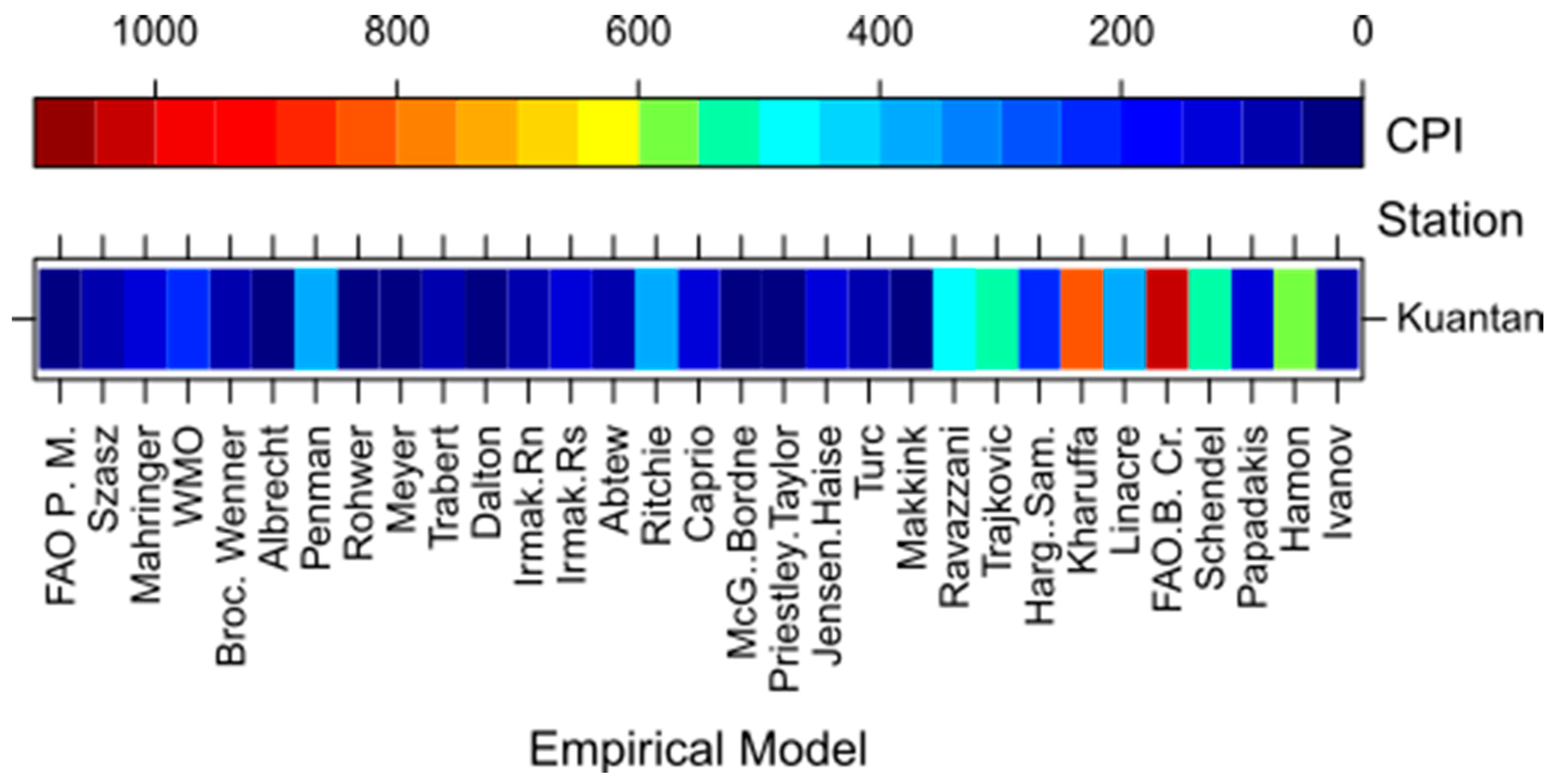
4.2. Compromise Programming

CP was employed to integrate the statistical metrics and rank the empirical models based on their capability in estimating the observed ET_o in Peninsular Malaysia. It was used to measure the distance of each empirical model from an ideal point at each station separately. As an example, the ideal results obtained at Kuantan station were the lowest NRMSE (93.10), the %BIAS nearest to zero (3.70) and, the highest md and KGE (0.58, for both). The CPI was calculated for each model through the summation of the subtraction of each metric from the ideal value. The following equation presents an example of the CPI calculation of the Ivanov model at Kuantan.

$$CP{I}_{KU,Ivanov}=\left|136.60-93.10\right|+\left|12.30-3.70\right|+\left|0.50-0.58\right|+\left|0.30-0.58\right|=52.46$$

(7)

The same procedure was used to calculate the CPI of the remaining models. Figure 4 shows a level plot of the CPI for each empirical model at Kuantan station.

4.3. Ranking the Empirical ET_o Models

Ranking of the empirical models was done through a six-step procedure, as stated in Section 3.4. First, the CPI values at each station were used to rank the empirical models, where the model that had the lowest CPI was ranked 1st at each station and vice versa. For example, the FAO Penman-Monteith model had the lowest CPI (7.60) in Kuantan station (refer to Figure 4), therefore ranked 1st, followed by the Dalton model which had the 2nd second lowest CPI of 20.08. The rank of each model at each station in Peninsular Malaysia is illustrated in Figure 5 as a level plot.

The frequency of occurrence that a model achieved a certain rank in different stations was calculated. For an example, the FAO Penman-Monteith model was found to have the least CPI in Kuala Terengganu, Kuantan, Melaka, and Muadzam Shah stations, so it was ranked 1st in these stations (refer to Figure 5). Therefore, the frequency of occurrence that the FAO Penman-Monteith model received as number one was four times. The levels of Figure 6 show the complete frequency of occurrence of the empirical models received a certain rank. For example, it can be seen that the FAO Penman-Monteith model was ranked at the 1st rank four times, 2nd rank once, 3rd rank four times, and 4th rank once. On the contrary, the FAO Blaney-Criddle and Kharuffa models were found to have the highest frequency (10 times) for getting the 31st and 30th rank, respectively.

The frequencies of occurrence of rank positions were multiplied by the rank weights and the overall score of each empirical model ($W_m$) was calculated by summing the output of the multiplication. For example, the frequencies of the FAO Penman-Monteith model having the 1st, 2nd, 3rd, and 4th rank were 4, 1, 4, and 1. So, the $W_m$ was calculated as shown in Equation (8).

$$W_{FAO P.-M.}=4\times 1^{-1}+1\times 2^{-1}+4\times 3^{-1}+1\times 4^{-1}=6.08$$

(8)

Based on the $W_m$, the models were finally ranked as shown in

Table 4. The overall weight achieved by the empirical ET_o models and their rank for entire Peninsular Malaysia.

Model	Wm	Final Rank	Model	Wm	Final Rank
FAO Penman-Monteith	6.08	1	Papadakis	0.58	17
Priestley-Taylor	3.54	2	WMO	0.57	18
Dalton	2.86	3	Caprio	0.55	19
Meyer	2.72	4	Irmak-Rs	0.55	20
Makkink	2.50	5	Jensen and Haise	0.51	21
Rohwer	2.40	6	Hargreaves and Samani	0.45	22
McGuinness and Bordne	1.98	7	Penman	0.44	23
Trabert	1.85	8	Linacre	0.41	24
Mahringer	1.79	9	Ritchie	0.41	25
Ivanov	1.62	10	Schendel	0.38	26
Albrecht	1.59	11	Ravazzani	0.38	26
Brockamp and Wenner	1.26	12	Trajkovic	0.36	28
Irmak-Rn	1.05	13	Hamon	0.35	29
Abtew	0.98	14	Kharuffa	0.33	30
Turc	0.74	15	FAO Blaney-Criddle	0.32	31
Szasz	0.71	16	-	-	-

. The FAO Penman-Monteith model was the top-ranked model in this study, followed by the Priestley-Taylor and Dalton models. The Hamon, Kharuffa, and FAO Blaney-Criddle models were ranked as the last three models.

The ranking of the ET models for different values of p is presented in

Table 5. Ranking of the empirical ET_o models for different values of p in compromise programming.

Model	p = 1	p = 2	p = ∞	Model	p = 1	p = 2	p = ∞
FAO Penman-Monteith	1	1	1	Papadakis	17	17	17
Priestley-Taylor	2	2	2	WMO	18	18	18
Dalton	3	5	4	Caprio	19	19	19
Meyer	4	4	3	Irmak-Rs	20	20	20
Makkink	5	3	5	Jensen and Haise	21	21	21
Rohwer	6	6	8	Hargreaves and Samani	22	23	22
McGuinness and Bordne	7	9	7	Penman	23	22	23
Trabert	8	7	6	Linacre	24	25	24
Mahringer	9	8	9	Ritchie	25	24	25
Ivanov	10	11	12	Schendel	26	27	27
Albrecht	11	10	10	Ravazzani	26	24	26
Brockamp and Wenner	12	12	11	Trajkovic	28	28	28
Irmak-Rn	13	20	15	Hamon	29	29	29
Abtew	14	14	13	Kharuffa	30	30	30
Turc	15	15	14	FAO Blaney-Criddle	31	31	31
Szasz	16	16	15	-	-	-	-

. The results revealed a slight variation in the ranks of a few models. From example, Makkink was ranked 5th for p = 1 and p = ∞, and it was ranked 3rd in case of p = 2. However, FAO Penman-Monteith was found as the most suitable method for all values of p. Priestley-Taylor was found best among the radiation-based models and Ivanov among the temperature-based models for all the cases. However, the best mass transfer-based model was not consistent for all values of p. Dalton was found best for p = 1, while Meyer was best for p = 2 and p = ∞. Therefore, both can be considered the most suitable mass transfer-based ET_o models for Peninsular Malaysia.

To show the efficacy of the top-ranked empirical model identified in this study, the FAO Penman-Monteith estimated and observed ET_o were compared. The heat scatter plots of observed FAO Penman-Monteith ET_o at different stations are presented in Figure 7. The figure shows that most of the points are aligned along the diagonal line, which indicates a perfect estimation of ET_o by FAO Penman-Monteith. The method overestimated ET_o in a few stations, such as Alor Star, Bayan Lepas, Kota Bahru, and Muadzam Shah.

5. Discussion

The FAO–Penman-Monteith method has been found as the most efficient for the estimation of ET_o in different climatic regions. The FAO Penman-Monteith model was developed based on physiological and aerodynamic theories of surface water release to the atmosphere. Therefore, it can be used as a standard model for estimation of ET_o in any region without any adjustment of parameters [24] based on the FAO recommendation [13,15]. The present study also found that FAO Penman-Monteith is the best model for Peninsular Malaysia. However, the Penman-Monteith model needs a large number of meteorological variables, including air temperature, wind speed, relative humidity, and solar radiation, for the estimation of ET_o. It is often very difficult to obtain data of all the meteorological variables. Many meteorological stations in the developing country do not measure all these variables. Therefore, a large number of alternative models have been developed based on the availability of data. The success of those models in a particular area often depends on the climate of the region. Therefore, the selection of an appropriate model based on the availability of data and the performance of ET_o estimation model is a difficult task. The performance of 31 empirical ET_o models has been assessed in this study. Input requirements of the models are different.

The performance of empirical ET_o models was often found to vary from station to station within the same climate zone, which may be due to the period and quality of data used, and uncertainty in the coefficient values used for the estimation of ET_o. Besides, suggesting different models for different stations often makes the practical application of the ET_o estimation model complex. Therefore, a single model is often suggested for the regional level for the estimation of ET_o. Thus, the ranking of ET_o estimation models in different stations was used in this study for the ranking of ET_o models for the entire Peninsular Malaysia using information aggregation approach.

In the present study, radiation-based Priestley and Taylor was found to perform best after the FAO Penman-Monteith model. It is followed by the mass transfer-based Dalton and Meyer models. The Priestley and Taylor model needs three meteorological variables (mean air temperature, solar radiation, and relative humidity) compared to the five variables required by the Penman-Monteith model (temperature, solar radiation, relative humidity, wind speed, and saturated vapor pressure), while Dalton and Meyer need three meteorological variables (mean temperature, relative humidity, and wind speed). Based on the availability of meteorological data, an appropriate model can be selected for the estimation of ET_o in Peninsular Malaysia with more or less similar accuracy.

Among the temperature-based models, only the Ivanov model was found to perform satisfactorily, which was ranked 10th among the 31 models compared in the present study. Other temperature-based models performed the worst and were ranked at the bottom of all the models. Many of the models were developed for a particular climate. For example, the Priestley and Taylor and the Makkink models were developed for the estimation of ET_o in a humid climate. On the other hand, the Turc model was found suitable for ET_o estimation in a cold, humid and arid climate [26]. Therefore, the Priestley and Taylor and Makkink models were found to perform very well among the radiation-based models, while Turc was found to perform worse than the simple temperature-based Ivonov model in tropical Malaysia.

The findings of the present study contradicts earlier studies. Ali and Lee [31] found Blaney–Criddle as the most suitable model after Penman-Monteith for the estimation of ET_o at Alor Setar station in Peninsular Malaysia. They only used relative error for the assessment of the performance of empirical ET_o models. Tukimat et al. [13] assessed the performance of seven empirical ET models for the same station using three statistical metrics, namely absolute error, relative error, and correlation coefficient. They found the least absolute and relative errors for the Hargreaves-Samani but highest correlation for Makkink, followed by Priestley-Taylor and Turc. They come to an overall conclusion that radiation-based models are most suitable for the estimation of ET_o in the region, which also support the findings of the present study. But they failed to decide the best model due to a contradiction in statistical metrics. Lee et al. [29] compared the performance of eight empirical models using mean absolute error, and reported FAO Blaney-Criddle as the most suitable model after FAO Penman-Monteith for estimation of ET_o in the west coast of the peninsula. Muniandy et al. [32] compared the performance of 26 empirical models at Senai station using eight statistical metrics. They also obtained contradictory results in term of different statistics. They took the arithmetic mean of the statistics to rank the models and found Penman as the best among the mass transfer-based models, McGuinness and Bordne among the radiation-based, and Szasz among the temperature-based models. Different models have been reported as the best in different stations in Peninsular Malaysia in the above studies, which do not match with the findings of the present study. This is due to the use of a single statistic for making a decision, as in the studies of Lee et al. [29] and Ali et al. [31]. Tukimat et al. [13] and Muniandy et al. [32] used multiple statistics, but did not attempt to find the best ET model based on the statistics. Muniandy et al. [32] attempted to rank the models based on the average of multiple statistics, but the average of statistics does not provide an optimum solution as the ranges of statistics metrics vary widely.

CP was used in this study for finding the most suitable empirical models based on four statistical metrics which can be used to measure the similarity between two time series in a robust way. CP proves a robust model compared to many MCDA models for finding a reliable solution based on multiple contradictory objectives. Therefore, the best empirical models identified in this study based on CP can be considered more reliable. Besides, the empirical models were ranked for the entire Peninsular Malaysia considering the fact of the same tropical humid climate for the whole region. The information aggregation model was used in this study for this purpose, which ranks the models based on the frequency of rank obtained by different models in different stations. Therefore, the top-ranked models in different stations were also found to achieve the top rank for the entire peninsula. This indicates the ranking of the models obtained in this study for the entire peninsula can be used for finding the most suitable model based on the availability of data for reliable estimation of ET_o.

6. Conclusions

The CP and GDM methods were used in this study for the ranking 31 ET_o empirical models for the estimation of ET_o in Peninsular Malaysia, based on four statistical metrics applied at 10 locations distributed over the study area. The result revealed Priestley and Taylor as the most suitable among the radiation-based models, Dalton among the mass transfer-based models, and Ivonov among the temperature-based models for the region. Though the mass transfer-based models were found more reliable compared to radiation-based models, Priestley and Taylor was found as the most suitable after Penman-Monteith, which is globally considered as the standard model for ET_o estimation. The Priestley and Taylor model needs only mean air temperature, solar radiation, and relative humidity compared to a large number of meteorological variables required for the estimation of ET_o using Penman-Monteith. Therefore, Priestley and Taylor can be used as a replacement of Penman-Monteith in the estimation of ET_o when available data is limited. The present study suggests that the Ivonov model, which requires only mean temperature and relative humidity, can be used for the worst case in terms of availability of data.

Estimation of ET_o in this study was based on pan coefficient of 0.75, as suggested by the Department of Irrigation and Drainage of Malaysia. The sensitivity of the ranking of ET_o estimation methods can be tested in the future for different pan coefficients. CP and GDM were used in this study for making a decision on ET_o models. Beside CP and GDM, other decision-making and information aggregation methods can be used, and their performance can be compared with the findings of the present study in the future. The parameters of the empirical models can be calibrated for Peninsular Malaysia before the comparison and ranking of the models.

References

1. Shahid, S. Impact of climate change on irrigation water demand of dry season boro rice in northwest Bangladesh. Clim. Chang. 2011, 105, 433–453. [Google Scholar] [CrossRef]
2. Jun, W.X.; Yun, Z.J.; Hua, W.J.; Min, H.R.; Elmahdi, A.; Hua, L.J.; Gong, W.X.; King, D.; Shahid, S. Climate Change and Water Resources Management in Tuwei River Basin of Northwest China. Mitig. Adapt. Strateg. Glob. Chang. 2012, 19, 107–120. [Google Scholar]
3. Wigmosta, M.S.; Vail, L.W.; Lettenmaier, D.P. A distributed hydrology-vegetation model for complex terrain. Water Resour. Res. 1994, 30, 1665–1679. [Google Scholar] [CrossRef]
4. Salem, G.; Kazama, S.; Shahid, S.; Dey, N. Impacts of Climate Change on Groundwater Level and Irrigation Cost in A Groundwater Dependent Irrigated Region. Agric. Water Manag. 2018, 208, 33–42. [Google Scholar] [CrossRef]
5. Mohsenipour, M.; Shahid, S.; Chung, E.S.; Wang, X.J. Changing pattern of droughts during cropping seasons of Bangladesh. Water Resour. Manag. 2018, 32, 1555–1568. [Google Scholar] [CrossRef]
6. Ismail, T.; Harun, S.; Zainudin, Z.M.; Shahid, S.; Fadzil, A.B.; Sheikh, U.U. Development of an optimal reservoir pumping operation for adaptation to climate change. KSCE J. Civ. Eng. 2017, 21, 467–476. [Google Scholar] [CrossRef]
7. Fisher, J.B.; Malhi, Y.; Bonal, D.; Da Rocha, H.R.; De Araujo, A.C.; Gamo, M.; Goulden, M.L.; Hirano, T.; Huete, A.R.; Kondo, H. The land—Atmosphere water flux in the tropics. Glob. Chang. Biol. 2009, 15, 2694–2714. [Google Scholar] [CrossRef]
8. Shiru, M.S.; Shahid, S.; Alias, N.; Chung, E.-S. Trend analysis of droughts during crop growing seasons of Nigeria. Sustainability 2018, 10, 871. [Google Scholar] [CrossRef]
9. Djaman, K.; Komlan, K.; Ganyo, K. Trend analysis in annual and monthly pan evaporation and pan coefficient in the context of climate change in togo. J. Geosci. Environ. Prot. 2017, 5, 41–56. [Google Scholar] [CrossRef]
10. Hadi Pour, S.; Abd Wahab, A.K.; Shahid, S.; Wang, X. Spatial pattern of the unidirectional trends in thermal bioclimatic indicators in Iran. Sustainability 2019, 11, 2287. [Google Scholar] [CrossRef]
11. Tukimat, N.N.A.; Harun, S.; Shahid, S. Modeling irrigation water demand in a tropical paddy cultivated area in the context of climate change. J. Water Resour. Plan. Manag. 2017, 143, 05017003. [Google Scholar] [CrossRef]
12. Irmak, S.; Allen, R.; Whitty, E. Daily grass and alfalfa-reference evapotranspiration estimates and alfalfa-to-grass evapotranspiration ratios in Florida. J. Irrig. Drain. Eng. 2003, 129, 360–370. [Google Scholar] [CrossRef]
13. Tukimat, N.N.A.; Harun, S.; Shahid, S. Comparison of different methods in estimating potential evapotranspiration at muda irrigation scheme of Malaysia. J. Agric. Rural Dev. Trop. Subtrop. 2012, 113, 77–85. [Google Scholar]
14. Lu, J.; Sun, G.; McNulty, S.G.; Amatya, D.M. A comparison of six potential evapotranspiration methods for regional use in the southeastern United States 1. JAWRA J. Am. Water Resour. Assoc. 2005, 41, 621–633. [Google Scholar] [CrossRef]
15. Djaman, K.; Balde, A.B.; Sow, A.; Muller, B.; Irmak, S.; N’Diaye, M.K.; Manneh, B.; Moukoumbi, Y.D.; Futakuchi, K.; Saito, K. Evaluation of sixteen reference evapotranspiration methods under sahelian conditions in the senegal river valley. J. Hydrol. Reg. Stud. 2015, 3, 139–159. [Google Scholar] [CrossRef]
16. Hasenmueller, E.A.; Criss, R.E. Multiple sources of boron in urban surface waters and groundwaters. Sci. Total Environ. 2013, 447, 235–247. [Google Scholar] [CrossRef] [PubMed]
17. Roudier, P.; Ducharne, A.; Feyen, L. Climate change impacts on runoff in West Africa: A review. Hydrol. Earth Syst. Sci. 2014, 18, 2789–2801. [Google Scholar] [CrossRef]
18. Ahmed, K.; Shahid, S.; Chung, E.S.; Ismail, T.; Wang, X.J. Spatial distribution of secular trends in annual and seasonal precipitation over Pakistan. Clim. Res. 2017, 74, 95–107. [Google Scholar] [CrossRef]
19. Jerszurki, D.; Souza, J.L.M.; Silva, L.C.R. Expanding the geography of evapotranspiration: An improved method to quantify land-to-air water fluxes in tropical and subtropical regions. PLoS ONE 2017, 12, e0180055. [Google Scholar] [CrossRef]
20. Gocic, M.; Trajkovic, S. Analysis of trends in reference evapotranspiration data in a humid climate. Hydrol. Sci. J. 2014, 59, 165–180. [Google Scholar] [CrossRef]
21. Thornthwaite, C.W. An approach toward a rational classification of climate. Geogr. Rev. 1948, 38, 55–94. [Google Scholar] [CrossRef]
22. Pereira, A.R.; Villa Nova, N.A.; Sediyama, G.C. Evapo(transpi)ração; FEALQ: Piracicaba, Brazil, 1997; p. 183. [Google Scholar]
23. Hamza, M.; Shahid, S.; Bin Hainin, M.R.; Nashwan, M.S. Construction labour productivity: Review of factors identified. Int. J. Constr. Manag. 2019, 19, 1–13. [Google Scholar] [CrossRef]
24. Lang, D.; Zheng, J.; Shi, J.; Liao, F.; Ma, X.; Wang, W.; Chen, X.; Zhang, M. A comparative study of potential evapotranspiration estimation by eight methods with fao penman—Monteith method in southwestern china. Water 2017, 9, 734. [Google Scholar] [CrossRef]
25. Song, X.; Lu, F.; Xiao, W.; Zhu, K.; Zhou, Y.; Xie, Z. Performance of twelve reference evapotranspiration estimation methods to penman-monteith method and the potential influences in northeast china. Meteorol. Appl. 2019, 26, 83–96. [Google Scholar] [CrossRef]
26. Tabari, H.; Grismer, M.; Trajkovic, S. Comparative analysis of 31 reference evapotranspiration methods under humid conditions. Irrig. Sci. 2011, 31, 107–117. [Google Scholar] [CrossRef]
27. Hosseinzadeh Talaei, P.; Tabari, H.; Abghari, H. Pan evaporation and reference evapotranspiration trend detection in western Iran with consideration of data persistence. Hydrol. Res. 2014, 45, 213–225. [Google Scholar] [CrossRef]
28. Bogawski, P.; Bednorz, E. Comparison and validation of selected evapotranspiration models for conditions in Poland (central europe). Water Resour. Manag. 2014, 28, 5021–5038. [Google Scholar] [CrossRef]
29. Lee, T.; Najim, M.; Aminul, M. Estimating evapotranspiration of irrigated rice at the west coast of the peninsular of Malaysia. J. Appl. Irrig. Sci. 2004, 39, 103–117. [Google Scholar]
30. Ali, M.H.; Lee, T.; Kwok, C.; Eloubaidy, A.F. Modelling evaporation and evapotranspiration under temperature change in Malaysia. Pertanika J. Sci. Technol. 2000, 8, 191–204. [Google Scholar]
31. Ali, M.H.; Shui, L.T. Potential evapotranspiration model for muda irrigation project, Malaysia. Water Resour. Manag. 2008, 23, 57. [Google Scholar] [CrossRef]
32. Muniandy, J.M.; Yusop, Z.; Askari, M. Evaluation of reference evapotranspiration models and determination of crop coefficient for momordica charantia and capsicum annuum. Agric. Water Manag. 2016, 169, 77–89. [Google Scholar] [CrossRef]
33. Allen, R.G.; Pereira, L.S.; Raes, D.; Smith, M. Crop evapotranspiration-guidelines for computing crop water requirements-fao irrigation and drainage paper 56. FaoRome 1998, 300, D05109. [Google Scholar]
34. Doorenbos, J.; Pruitt, W. Crop Water Requirements. FAO Irrigation and Drainage Paper 24; Land and Water Development Division, FAO: Rome, Italy, 1977. [Google Scholar]
35. Nashwan, M.S.; Shahid, S.; Wang, X. Assessment of satellite-based precipitation measurement products over the hot desert climate of Egypt. Remote Sens. 2019, 11, 555. [Google Scholar] [CrossRef]
36. Nashwan, M.S.; Shamsuddin, S.; Wang, X.-J. Uncertainty in estimated trends using gridded rainfall data: A case study of Bangladesh. Water 2019, 11, 349. [Google Scholar] [CrossRef]
37. Nashwan, M.S.; Shahid, S. Symmetrical uncertainty and random forest for the evaluation of gridded precipitation and temperature data. Atmos. Res. 2019, 230, 104632. [Google Scholar] [CrossRef]
38. Zeleny, M. Compromise Programming, Multiple Criteria Decision-Making. In Multiple Criteria Decision Making; University of South Carolina Press: Columbia, SC, USA, 1973; pp. 263–301. [Google Scholar]
39. Rezaei, F.; Ahmadzadeh, M.R.; Safavi, H.R. Som-drastic: Using self-organizing map for evaluating groundwater potential to pollution. Stoch. Environ. Res. Risk Assess. 2017, 31, 1941–1956. [Google Scholar] [CrossRef]
40. Salman, S.A.; Shahid, S.; Ismail, T.; Al-Abadi, A.M.; Wang, X.-J.; Chung, E.-S. Selection of gridded precipitation data for iraq using compromise programming. Measurement 2019, 132, 87–98. [Google Scholar] [CrossRef]
41. Chen, W.; Wiecek, M.M.; Zhang, J. Quality utility—A compromise programming approach to robust design. J. Mech. Des. 1999, 121, 179–187. [Google Scholar] [CrossRef]
42. Srinivasa Raju, K.; Sonali, P.; Nagesh Kumar, D. Ranking of CMIP5-based global climate models for India using compromise programming. Theor. Appl. Climatol. 2017, 128, 563–574. [Google Scholar] [CrossRef]
43. Nashwan, M.S.; Shahid, S. Spatial distribution of unidirectional trends in climate and weather extremes in Nile river basin. Theor. Appl. Climatol. 2019, 137, 1181–1199. [Google Scholar] [CrossRef]
44. Nashwan, M.S.; Shahid, S.; Abd Rahim, N. Unidirectional trends in annual and seasonal climate and extremes in Egypt. Theor. Appl. Climatol. 2019, 136, 457–473. [Google Scholar] [CrossRef]
45. Nashwan, M.S.; Ismail, T.; Ahmed, K. Non-stationary analysis of extreme rainfall in peninsular Malaysia. J. Sustain. Sci. Manag. 2019, 14, 17–34. [Google Scholar]
46. Nashwan, M.S.; Ismail, T.; Ahmed, K. Flood susceptibility assessment in Kelantan river basin using copula. Int. J. Eng. Technol. 2018, 7, 584–590. [Google Scholar] [CrossRef] [Green Version]
47. Nashwan, M.S.; Shahid, S.; Chung, E.-S.; Ahmed, K.; Song, Y.H. Development of climate-based index for hydrologic hazard susceptibility. Sustainability 2018, 10, 2182. [Google Scholar] [CrossRef]
48. Tangang, F.T. Low frequency and quasi-biennial oscillations in the Malaysian precipitation anomaly. Int. J. Climatol. 2001, 21, 1199–1210. [Google Scholar] [CrossRef]
49. Brouwer, C.; Heibloem, M. Irrigation Water Management: Irrigation Water Needs. Training Manual; FAO: Rome, Italy, 1986; Volume 3. [Google Scholar]
50. DID. Evaporation in Peninsular Malaysia, 1st ed.; Department of Irrigation and Drainage (DID) Malaysia: Kuala Lumpur, Malaysia, 1976; Volume 5.
51. Romanenko, V. Computation of the autumn soil moisture using a universal relationship for a large area. Proc. Ukr. Hydrometeorol. Res. Inst. 1961, 3, 12–25. [Google Scholar]
52. Hamon, W.R. Computation of direct runoff amounts from storm rainfall. Int. Assoc. Sci. Hydrol. Publ. 1963, 63, 52–62. [Google Scholar]
53. Papadakis, J. Crop Ecologic Survey in Relation to Agricultural Development of Western Pakistan; Draft Report; FAO: Rome, Italy, 1965. [Google Scholar]
54. Schendel, U. Vegetations wasserverbrauch und-wasserbedarf. Habilitation, Kiel, 1967; 137p. [Google Scholar]
55. Linacre, E.T. A simple formula for estimating evaporation rates in various climates, using temperature data alone. Agric. Meteorol. 1977, 18, 409–424. [Google Scholar] [CrossRef]
56. Kharrufa, N. Simplified equation for evapotranspiration in arid regions. Beiträge Hydrol. 1985, 5, 39–47. [Google Scholar]
57. Hargreaves, G.H.; Samani, Z.A. Reference crop evapotranspiration from temperature. Appl. Eng. Agric. 1985, 1, 96–99. [Google Scholar] [CrossRef]
58. Trajkovic, S. Hargreaves versus penman-monteith under humid conditions. J. Irrig. Drain. Eng. 2007, 133, 38–42. [Google Scholar] [CrossRef]
59. Ravazzani, G.; Corbari, C.; Morella, S.; Gianoli, P.; Mancini, M. Modified hargreaves-samani equation for the assessment of reference evapotranspiration in alpine river basins. J. Irrig. Drain. Eng. 2011, 138, 592–599. [Google Scholar] [CrossRef]
60. Makkink, G. Testing the penman formula by means of lysimeters. J. Inst. Water Eng. 1957, 11, 277–288. [Google Scholar]
61. Turc, L. Water Requirements Assessment of Irrigation, Potential Evapotranspiration: Simplified and Updated Climatic Formula; Annales Agronomiques: Paris, France, 1961; pp. 13–49. [Google Scholar]
62. Jensen, M.E.; Haise, H.R. Estimating evapotranspiration from solar radiation. Proc. Am. Soc. Civ. Eng. J. Irrig. Drain. Div. 1963, 89, 15–41. [Google Scholar]
63. Priestley, C.H.B.; Taylor, R. On the assessment of surface heat flux and evaporation using large-scale parameters. Mon. Weather Rev. 1972, 100, 81–92. [Google Scholar] [CrossRef]
64. McGuinness, J.L.; Bordne, E.F. A Comparison of Lysimeter-Derived Potential Evapotranspiration with Computed Values; U.S. Department of Agriculture: Washington, DC, USA, 1972.
65. Caprio, J.M. The solar thermal unit concept in problems related to plant development and potential evapotranspiration. In Phenology and Seasonality Modeling; Springer: Berlin/Heidelberg, Germany, 1974; pp. 353–364. [Google Scholar]
66. Jones, J.W.; Ritchie, J.T. Crop growth models. In Management of Farm Irrigation Systems; Hoffman, G.J., Howel, T.A., Solomon, K.H., Eds.; ASAE: Washington, DC, USA, 1990; pp. 63–69. [Google Scholar]
67. Abtew, W. Evapotranspiration measurements and modeling for three wetland systems in south Florida. J. Am. Water Resour. Assoc. 1996, 32, 465–473. [Google Scholar] [CrossRef]
68. Dalton, J. Experimental essays on the constitution of mixed gases; on the force of steam or vapor from water and other liquids in different temperatures, both in a torricellian vacuum and in air; on evaporation and on the expansion of gases by heat. Mem. Lit. Philos. Soc. Manch. 1802, 5, 535–602. [Google Scholar]
69. Trabert, W. Neue beobachtungen über verdampfungsgeschwindigkeiten [new observations on evaporation rates]. Met. Z. 1896, 13, 261–263. [Google Scholar]
70. Meyer, A. Über einige zusammenhänge zwischen klima und boden in Europa. ETH Zur. 1926, 2, 209–347. [Google Scholar]
71. Rohwer, C. Evaporation from Free Water Surfaces; US Department of Agriculture: Washington, DC, USA, 1931.
72. Penman, H.L. Natural evaporation from open water, bare soil and grass. Proc. R. Soc. London Ser. A Math. Phys. Sci. 1948, 193, 120–145. [Google Scholar] [Green Version]
73. Albrecht, F. Die methoden zur bestimmung der verdunstung der natürlichen erdoberfläche. Arch. Meteorol. Geophys. Und Bioklimatol. Ser. B 1950, 2, 1–38. [Google Scholar] [CrossRef]
74. Brockamp, B.; Wenner, H. Verdunstungsmessungen auf den Steiner see bei münster. Dt Gewässerkundl Mitt 1963, 7, 149–154. [Google Scholar]
75. Gangopadhyaya, M. Measurement and Estimation of Evaporation and Evapotranspiration; WMO: Geneva, Switzerland, 1966. [Google Scholar]
76. Mahringer, W. Verdunstungsstudien am neusiedler see. Arch. Meteorol. Geophys. Und Bioklimatol. Ser. B 1970, 18, 1–20. [Google Scholar] [CrossRef]
77. Szasz, G. A potenciális párolgás meghatározásának új módszere. Hidrol. Közlöny 1973, 10, 435–442. [Google Scholar]
78. Willmott, C.J. Some comments on the evaluation of model performance. Bull. Am. Meteorol. Soc. 1982, 63, 1309–1313. [Google Scholar] [CrossRef]
79. Gupta, H.V.; Kling, H.; Yilmaz, K.K.; Martinez, G.F. Decomposition of the mean squared error and nse performance criteria: Implications for improving hydrological modelling. J. Hydrol. 2009, 377, 80–91. [Google Scholar] [CrossRef]
80. Gorantiwar, S.; Smout, I.K. Multicriteria Decision Making (Compromise Programming) for Integrated Water Resources Management in an Irrigation Scheme; Loughborough University Institutional Repository: Leicestershire, UK, 2010. [Google Scholar]
81. Perez-Verdin, G.; Monarrez-Gonzalez, J.C.; Tecle, A.; Pompa-Garcia, M. Evaluating the multi-functionality of forest ecosystems in northern Mexico. Forests 2018, 9, 178. [Google Scholar] [CrossRef]
82. Tecle, A.; Shrestha, B.P.; Duckstein, L. A multiobjective decision support system for multiresource forest management. Group Decis. Negot. 1998, 7, 23–40. [Google Scholar] [CrossRef]
83. Ahmed, K.; Shahid, S.; Sachindra, D.A.; Nawaz, N.; Chung, E.-S. Fidelity assessment of general circulation model simulated precipitation and temperature over Pakistan using a feature selection method. J. Hydrol. 2019, 573, 281–298. [Google Scholar] [CrossRef]
84. Srinivasa Raju, K.; Nagesh Kumar, D. Ranking general circulation models for India using topsis. J. Water Clim. Chang. 2015, 6, 288–299. [Google Scholar] [CrossRef]
Figure 1. The geographical location of Peninsular Malaysia and the selected meteorological station used in this study. Description of the stations is given in Table 1.
Sustainability 11 04267 g001
Figure 2. Heat-scatter plots of the observed ETo against the estimation of empirical models (aae).
Sustainability 11 04267 g002
Figure 3. Box plot of (a) normalized root mean square error (NRMSE), (b) percentage of bias (%BIAS), (c) modified index of agreement (md), and (d) Kling-Gupta efficiency (KGE) obtained for different empirical models in estimating the ETo. The blue, green, gold, and pink box plots represent the temperature-based, radiation-based, mass transfer-based, and combination-based models, respectively. The red vertical lines represent the optimum value of each metric.
Sustainability 11 04267 g003
Figure 4. The compromise programming index (CPI) of the empirical models at Kuantan station. The FAO Penman-Monteith model had the lowest CPI (7.60), while the FAO Blaney-Criddle model had the highest CPI (1043.44).
Sustainability 11 04267 g004
Figure 5. Ranking of the empirical models at 10 stations in Peninsular Malaysia according to their CPI (p = 1).
Sustainability 11 04267 g005
Figure 6. The level plot showing the frequency of occurrence of the empirical models for different ranks.
Sustainability 11 04267 g006
Figure 7. Heat-scatter plots of the observed ETo and the estimated ETo by the FAO Penman-Monteith model at (a) Alor Star; (b) Bayan Lepas; (c) Ipoh; (d) Kota Bharu; (e) Kuala Terengganu; (f) Kuantan; (g) Melaka; (h) Muadzam Shah; (i) Senai; and (j) Subang.
Sustainability 11 04267 g007