1. Introduction
Nowadays, a wide consensus has been achieved upon the importance of good architectural design and its relationship with energy consumption [
1]. As a matter of fact, energy efficiency in the residential sector is one of the priority objectives of the European Union, which in the Directive 2010/31/EU requires 20% reduction in emissions of global warming gases, 20% reduction in energy consumption, and 20% increment in the use of renewable energies with respect to 1990 levels [
2].
It is estimated that energy savings up to 27% will be achieved in residential buildings by 2020 as per Directive 2012/27/EU and Directive 2018/844/UE [
3,
4]. The impact of buildings is significant, and amounts to approximately 40% of global energy consumption and one third of global greenhouse gas (GHG) emissions [
5].
When it comes to the construction of dwellings in the Spanish Mediterranean area, what is found is a general and widespread lower energy efficiency than other countries within the European Union facing the Mediterranean basin [
6].
In typical Spanish dwellings, energy consumption due to heating and cooling represents approximately 48% of the total energy used [
7]. To help architects and designers reduce the operational energy consumption of buildings, the Spanish Technical Building Code (CTE) recommends the application of a tool called LIDER-CALENER GT (HULC) [
8,
9]. Such a tool is used to verify the compliance of the project with the prescriptions set by CTE’s basic document DB-HE, as well as for evaluating the energy demand with respect to the DB-HE1’s requirements (item 2.2.1) regarding the limitation of the energy demand in residential buildings.
In the light of the above, the Passive House standard is rapidly spreading all over the world with approximately 25,000 passive houses in use worldwide [
10]. Several authors [
11,
12,
13] claim that they can save up to 50% of the total primary energy consumption. A comparison between certified passive houses and generic low-energy houses revealed that passive house CO
2 emissions were approximately 25–40% lower, with only a 5% of increase in initial construction costs [
14].
Various studies indicate that passive design measures and orientation have a considerable influence on energy efficiency, comfort and safety. There are several researches work whose objective is to discuss the implementation of passive strategies in order to reduce the energy demand in buildings [
15,
16,
17].
An adequate practice of passive design involves several aspects of building design [
18,
19] such as the orientation of the main façades and windows, the choice of appropriate walls’ materials, thermal insulation and Window-to-Wall Ratio (WWR), along with the design of shading devices and the implementation of natural ventilation techniques [
20,
21,
22,
23,
24].
The PH concept furthers the traditional passive building approach by improving thermal comfort conditions at minimum energy costs [
25]. The distinctive features of the PH standard, as prescribed in the updated official website [
26,
27], are:
Space heating demand: not to exceed 15 kWhm−2 annually or not to exceed 10 Wm−2 of peak demand;
Space cooling demand: matches the heat demand requirements with an additional, climate—dependent allowance for dehumidification;
Primary energy demand: not to exceed 120 kWhm−2 annually for all domestic applications (heating, cooling, hot water and domestic electricity);
Air tightness: air leakages should be kept below 0.6 air changes per hour at 50 Pa pressure difference (to assess on—site through a blower—door test).
Thermal comfort for summer operation: a maximum of 10% of hours in a year exceeding 25 °C can be accepted (overheating criterion);
High thermal insulation values in all components of the building envelope (typical U values between 0.6 and 0.15 Wm−2K−1).
The vast majority of passive structures have been built in northern and central European countries, but there is a significant interest for research and development targeted to the adaptation of passive houses under different climatic conditions, especially for the Mediterranean climate. In this sense, the standard allows for exceeding the overheating temperature threshold of 25 °C for no more than 10% of the cooling period in warmer climates [
28]. The main problem when adapting buildings on the Mediterranean coast to the PH standard is that cooling needs must be taken into great account in summer in addition to heating demands in winter [
29]. This research aims to highlight the effectiveness of the application of passive house principles on new buildings in the early design stage of residential buildings projects in the Mediterranean zone. Applying the principles of passive design to new buildings costs little or nothing while also responding to local climate and site conditions to maximize building users’ comfort and health while minimizing energy use. Architects, designers, builders and stakeholders have to be aware of the opportunity raising from incorporating the principles of passive houses in the early stages of a project. Moreover, the large number of opportunities in the market today makes necessary for architects and designers to have a tool to assist them in identifying the best combinations for any specific situation [
30] in order to determine which design strategy should be pursued more actively to achieve better energy performance. In this context, energy simulation is a powerful tool to improve building design [
31]. The use of Building Performance Simulation Tools (BPSTs) offers the architects and designers In general a thorough understanding of the impact of several design variables [
32]. This sort of simulations cannot be carried out using semi steady state tool like the Passive House Planning Package (PHPP, [
33]) when it comes to consider a building’s summer behavior and thus inertial effects. With this in mind, parametric energy dynamic simulations were performed to evaluate the effectiveness of passive house measures on new building design located in Spain with different climate conditions.
Despite the importance of using BPSTs, most architects and designers committed to design passive and low-energy buildings still do not use such tools, but rather rely on basic rules and environmental design guidelines [
34,
35,
36]. Due to this reason, communication with software developers is often deficient [
37]. Technical and non-technical barriers have been detected that prevent adopting BPSTs in the context of design, and producing a usage gap that will only begin to be solved when users will be prepared to properly interpret the results of simulations [
38]. Since the late 1990s, software developers and researchers have tried to provide efficient visualization systems in which designers can easily compare and evaluate alternatives along with their proposals [
39,
40]. In order to understand the results of a simulation and make design decisions based on them, there is a need to research these aspects of architectural design [
41,
42]. There are examples of data visualizations which relate the decision-making process of design with objectives [
43]. A powerful and meaningful way to explore several design solutions, and their impact on the resulting operational energy demand, is given by a parametric analysis of selected key variables [
44]. The parametric sensitivity analysis is used to understand how the input parameters propagate through the model [
45]; it is usually accomplished by assigning ranges of values in order to “evaluate the influence or relative importance of each input and output” [
46]. In order to facilitate the interpretation of data, users must be provided with the ability to compare and relate information [
47]. In the following research work, two main objectives are taken into account. The first objective is to provide building designers with suggestions for the achievement of low-energy building design within the five climate zones in Spain through the use of passive strategies. The second one is to help designers understand the complexity of the simulation outcomes through graphic representations that relates the results of the simulations with architectural design decisions.
2. Methodology
The research aims to highlight the effectiveness of the application of passive house principles on new buildings. To this purpose, parametric energy dynamic simulations were performed to evaluate the effectiveness of passive house measures on new buildings located in Spain under different climate conditions.
In this section, the different types of buildings representative of typical house dwellings in Spain are first introduced and discussed. Then, the design parameters taken into account for running a parametric analysis of different design options are presented. Finally, the different climate conditions pertaining to several climate zones where the buildings are simulated are explained.
2.1. Building Types and Simulation Parameters
In order to consider the building types that are most representative of the residential building stock in Spain, the classification resulting from the analysis of statistical data obtained from the Rehenergía project [
48] and from the Spanish National Statistics Institute (INE data base [
49]) has been used, with a focus on multi-dwelling units (MDUs). This is why the resulting simulation space does not take into account further variations possible through a brute-force parametric approach.
Table 1 shows the building types analyzed in this research. They are the AT1b with a prominent linear shape, and the AT2 and AT3 types that are both cubic and hollow but show different shape factors (i.e. different ratios of the heat transfer surface to the enclosed volume).
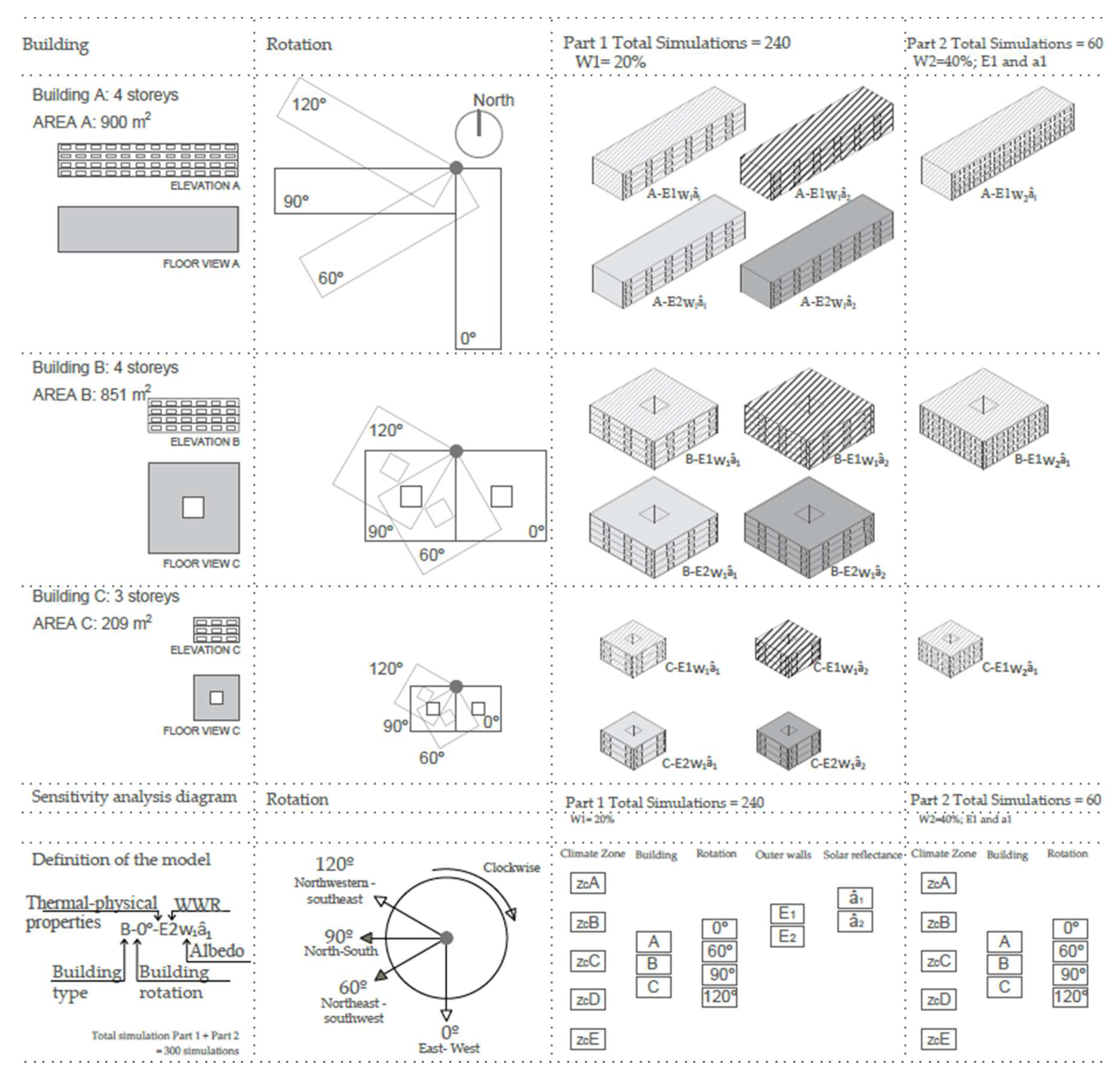
As mentioned in the introduction, the study is based on dynamic simulations carried out using the Energy Plus software through the Design Builder graphical interface [
50]. A total number of 300 simulations are accomplished. A first set of simulations-for a total number of 240 models-considers the parametric variations of climate zones (5), building types (3), building orientation (4), U-values of external walls (2) and their external solar reflectance values (2). For such group of simulations, the parameter held constant is the Window-to-Wall Ratio (WWR), for which a constant value of 20% has been used for all facades. On the other hand, the second set of simulations includes 60 models and considers the parametric variations of climate zones (5), building types (3) and building orientation (4). The parameters considered constant in this case are the WWR (40% for all the facades), the U-value for the external walls (U = 1.58 Wm
−2K
−1) and walls solar reflectance (equal to 0.64). All these variations are summarized in
Figure 1.
Table 2 summarizes all the simulation parameters, mostly referring to the Spanish regulations in force [
6]. Simulations are carried out using the set back and set point temperature schedules presented in
Table 3, i.e., heating and cooling ideal loads air systems are supposed to be in use whenever needed for keeping indoor air temperature within the temperature ranges set (17 to 20 °C in winter and 25 to 27 °C in summer respectively).
The first parameter considered is the orientation. The different orientations selected for the models are taken from the Spanish Building Technical Code (SBTC). In order to define the type of orientation of the different models, the 0° value corresponds to the East-West orientation whereas the 60° value corresponds to the Northeast-Southwest orientation. In addition, the value equal to 90° corresponds to the North-South orientation and the 120° value is related to the Northwest-Southeast orientation.
The second parameter considered is the overall heat transfer coefficient (U-value, Wm
−2K
−1), which determines the heat loss through the unit area of the envelope elements. It is common that regulations impose a maximum U-value to control the heat loss of buildings and thus ensure reduced energy consumption for heating and cooling. Since 68% of the current building stock in Spain was constructed before 1979 [
51], two different thermal transmittance values are considered for the external walls, while keeping the U-values pertaining to the roof and to the windows as constant. The value of 1.58 Wm
−2K
−1 corresponds to those buildings constructed before the above mentioned regulation came into force, and the value of 0.35 Wm
−2K
−1 that corresponds to those built later.
Table 4 describes all the transmittance values of walls, roof, and windows in order. Roof with a slope wasn’t analyzed because its parametric modeling can cause numerical problems during the simulations [
52,
53,
54].
As far as solar reflectance is concerned, two different values have been considered: â1 = 0.64 that corresponds to a light beige color, and the value â2 = 0.2 that corresponds to a generic darker color.
The last parameter varied during the simulations is the Window-to-Wall Ratio (WWR). The WWR in the façade is a determining factor in terms of heat gains and losses through glazed surfaces. In order to define this variable, SBTC 2006 is taken as a reference. The percentages selected range from 21 to 30% and from 31 to 40%. It is considered that these values cover the usual spectrum of WWR in Spain [
9].
2.2. Selection of Different Climate Zones
Research indicates that improving the insulation of buildings or saving the energy obtained from conventional sources must not be abandoned [
11,
12,
13] Therefore, buildings with solar and cooling adaptation systems must be built since they are more effective in a climate like that of Spain. During the coldest winter month, i.e., January, 50% of Spanish cities could be heated with active and passive solar energy throughout the day. The remaining would need conventional heating only during the night. In an average winter month, such as November or March, 90% of the Spanish cities could be heated with solar contributions from passive and active systems. 80% of them would be worth heating only with passive solutions during the central hours of the day. In the hottest months, such as July in the interior zone or August on the coast areas, comfort conditions can be obtained in buildings by means of ventilation in the wettest areas, i.e., 26% of the cities. 56% of the other cities could be heated if buildings were capable of maintaining nighttime temperatures during the day. This is possible because the oscillation of temperatures ranges from 16 °C to 23 °C. Therefore, very few cities in Spain would need to consume energy in air conditioning under good conditions of mass and thermal inertia in buildings [
16].
The climate zones established in the Basic Document of Energy Saving pertaining to the Technical Building Code (DB-H) [
9] have been identified according to expected energy demand of buildings and gave rise to a total of 17 zones. Twelve of these zones are peninsular zones (established since 2006), namely those tagged as A3, A4, B3, B4, C1, C2, C3, C4, D1, D2, D3, and E1. In 2013, five specific climate zones were introduced corresponding to the Canary Islands (Alpha 1, 2, and 3, A2, and B2).
The nomenclature used defines the zones with a combination of its Winter Climate Severity (letter, α, A, B, C, D, E from the mildest to the coldest winter), and its Summer Climate Severity (number, 1–4, from the mildest to the hottest summer). The concept of climate severity is defined as the ratio of the energy demand of a building to that of the same building in a reference location.
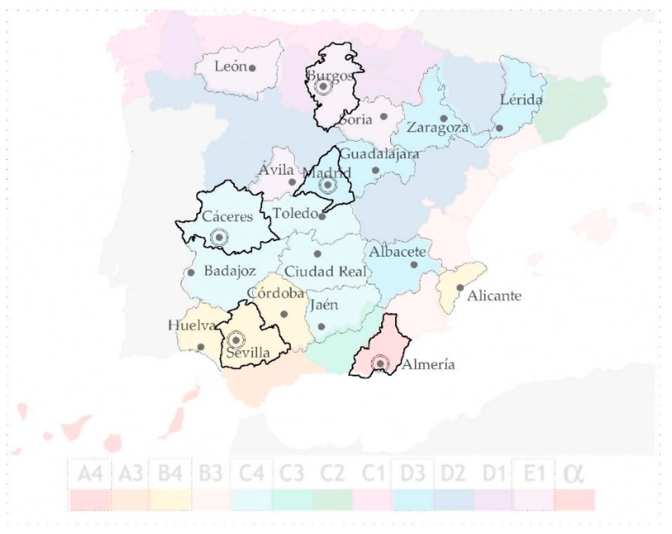
In this work, five climate zones out of the 17 zones are selected. The maximum numerical value (numbers 1 to 4) is selected within each climate zone. It corresponds to the highest temperatures during the summer. Therefore, the selection of zones A4, B4, C4, D3, and E1 is considered. The representative cities for each zone are Almeria (latitude 36.85, longitude –2.38) within zone A4 and Seville (latitude 37.42, longitude –5.9) within zone B4. Caceres (latitude 39.47, longitude —6.33), Madrid (latitude 40.45, longitude –3.55), and Burgos (latitude 42.35, longitude –3.67) are considered within climate zones C4, D3, and E1 respectively (see
Figure 2).
Table 5 lists the main features of the selected climate zones. Their Heating Degree Days (HDD) and Cooling Degree Days (CDD) are first calculated on the basis of 20 and 25 °C respectively, while dry bulb temperature, relative humidity and global horizontal radiation values are presented for both the summer (from June to September) and the winter (January to March and October to December) periods as average seasonal values.
3. Results and Discussion
This section presents the results of the 300 simulations carried out for the different climate zones. The best and worst thermal models for each climate conditions are shown and commented, as well as the characteristics that mostly influence their energy demand. Finally, a comparison of the results according to the different climates and with respect to the PH standard compliance is reported.
3.1. Models Calibration and Graphical Presentation of the Results
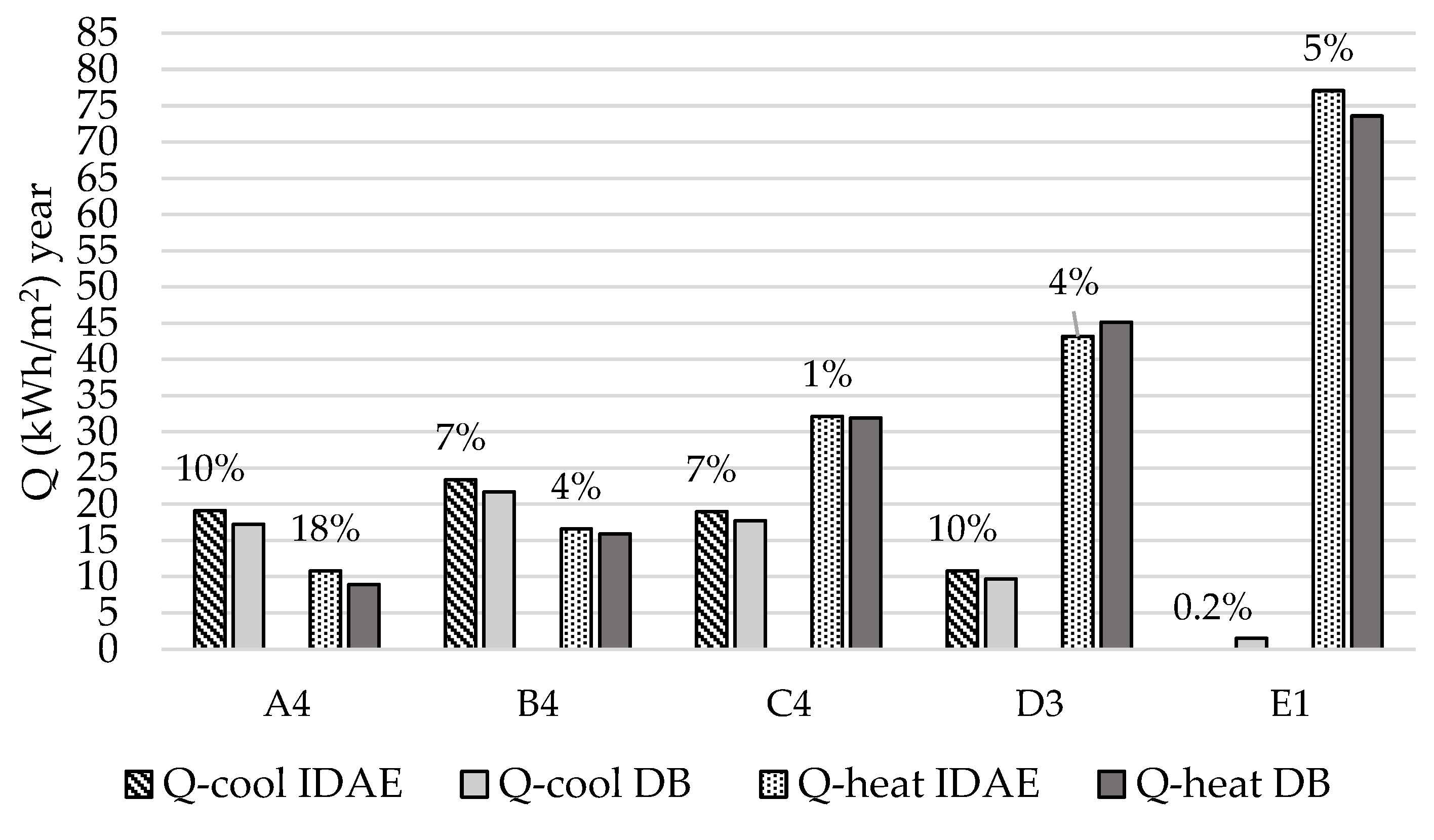
As a measure of quality control of the simulations outcomes, the results of this research have been preliminary checked against the values established by the Spanish Institute of Energy Diversification and Saving (IDAE), which has determined the energy consumption and costs of the Spanish households thanks to in situ measurements of about 600 households in different climate zone of Spain. Such values can be considered as reference for both the heating and cooling demands in multi—dwelling units [
55,
56]. The Design Builder (DB) values presented in
Figure 3 correspond to the average of the 300 models simulated. As it can be seen, the average values obtained with DB simulations are very close to those obtained from IDAE. The biggest difference is found when estimating the space heating demand in climate zone A4 (18% difference).
Given the high number of simulations and the amount of resulting data, great attention has been paid also to the presentation of the results in a concise manner. As the purpose of this study is to examine the energy demand linked to the architectural design, the results are presented mainly through histograms and relying on the nomenclature and symbols defined in
Section 2.1 that help to link the design strategy with the numerical results. The value equal to 15 kWhm
−2, and relevant to the PH standard energy demand threshold, has also been reported in the graphs in order to easily appreciate the fulfillment of the requirement.
Finally, the criterion chosen for defining the best design solution is that of the lowest energy demand for cooling (Q-cool), heating (Q-heat) and total (heating and cooling, Q). The opposite applies for identifying the worst design solutions.
3.2. Climate Zone A4
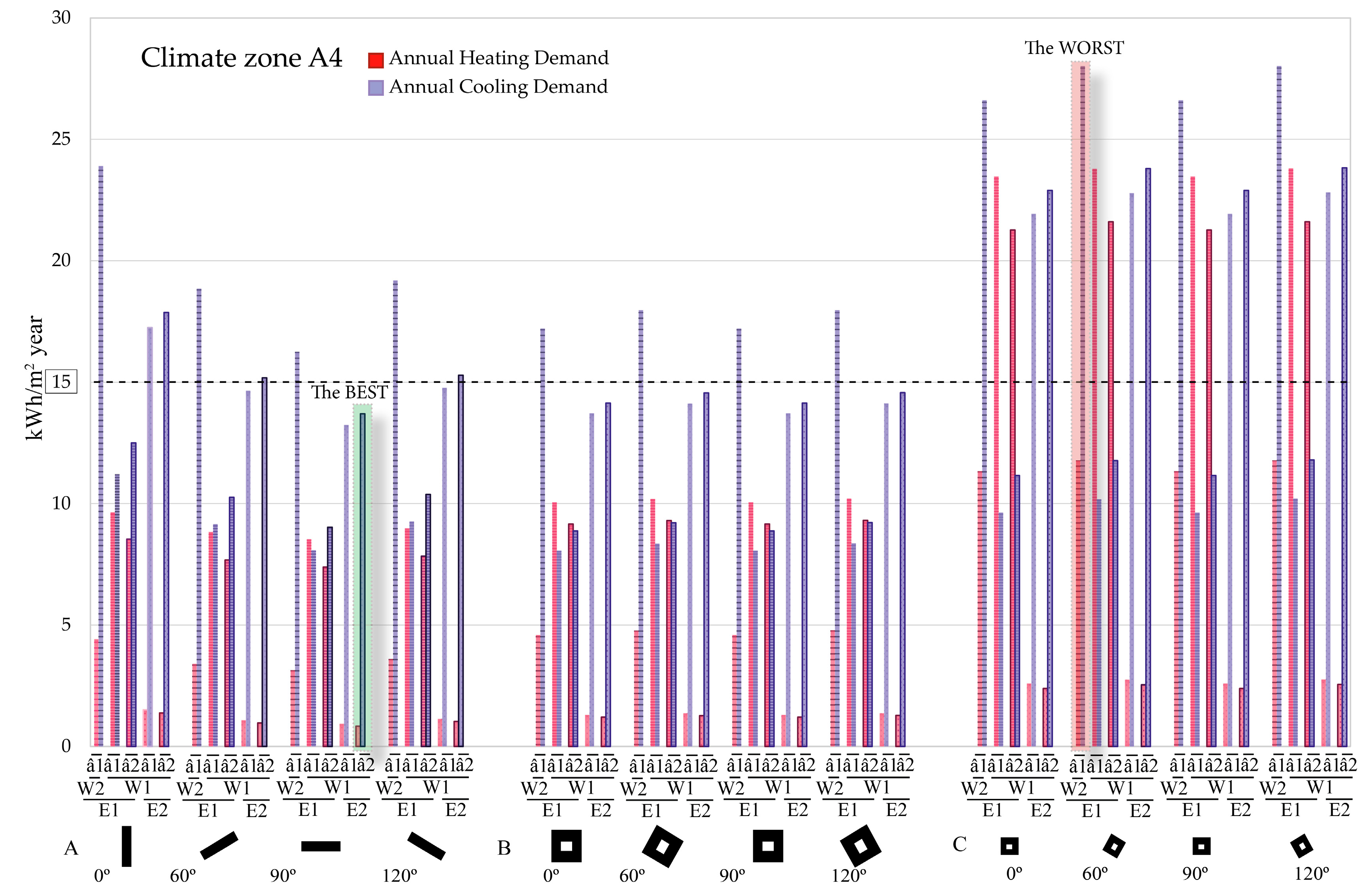
Figure 4 shows that the lowest heating energy demand is associated to model A (Q-heat = 0.84 kWhm
−2) when rotated 90° using envelope E2 (U = 0.35 Wm
−2K
−1), as well as a WWR equal to W1 (20%), dark colors â
2 (0.2), and a lower shape factor (0.26). On the other hand, the lowest cooling energy demand (Q-cool = 8.06 kWhm
−2) is associated to model B when rotated 0° and 90° using envelope E1 (U = 1.58 Wm
−2K
−1), as well as a WWR equal to W1 (20%), light colors â
1 (0.8), and a lower shape factor (0.26). Therefore, the optimal design parameters when considering both the heating and the cooling energy demands happen to occur when lower shape factors (0.26) and a lower WWR (20%) are taken into account.
The worst model when considering the heating energy demand (Q-heat = 23.80 kWhm
−2) corresponds to model C when rotated 120° from the North using envelope E1 (U = 1.58 Wm
−2K
−1), as well as a WWR equal to W1 (20%), light colors â
1 (0.8), and a greater shape factor (0.48). As for the cooling energy demand, the highest value (Q-cool = 28.02 kWhm
−2) is associated to model C when rotated 60° and 120° from the North using envelope E1 (U = 1.58 Wm
−2K
−1), as well as a WWR equal to W2 (40%), light colors â
1 (0.8), and a greater shape factor (0.48). Due to this fact, the higher the WWR (0.48), the greater the amount of solar radiation penetrating the interior of the building and therefore the more cooling energy demand needed [
55].
On the other hand, when it comes to the appraisal of the total energy demand, the best model coincides with the best one pertaining to the lowest heating energy demand, except for the solar reflectance (â). In this particular case, the best model includes using light façade colors (â1 = 0.8) with a value of the overall consumption equal to Q = 14.17 kWhm−2. However, the worst model corresponds to model C (Q = 39.80 kWhm−2) when rotated 60° and 120° from the North using envelope E1 (U = 1.58 Wm−2K−1), as well as a WWR equal to W2 (40%), light colors â1 (0.8), and a greater shape factor (0.48). Therefore, the worst model with regard to the total energy demand coincides with the lowest cooling energy demand.
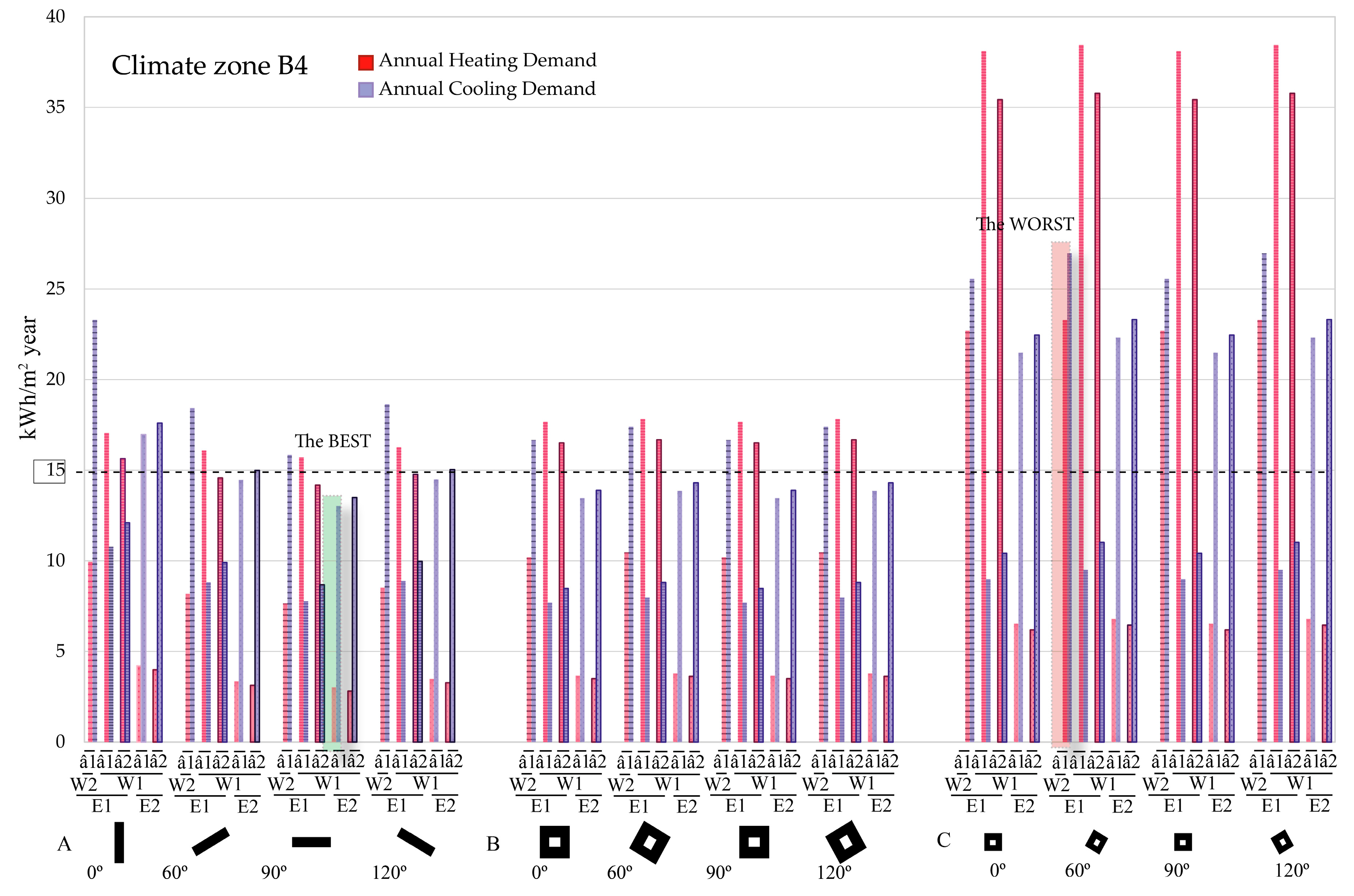
3.3. Climate Zone B4
Figure 5 shows the analysis of the results pertaining to climate zone B4. The best model within zone B4 regarding the lowest heating energy demand is associated to model A when rotated 90° using envelope E2 (U = 0.35 Wm
−2K
−1), as well as a WWR equal to W1 (20%), dark colors â
2 (0.2), and a lower shape factor (0.26). It corresponds to the same model and characteristics relevant to that of climate zone A4. In this particular case, the value of the heating energy demand equals 2.81 kWhm
−2. Such value doubles that of climate zone A4. As for the best model pertaining to the lowest cooling energy demand, it is associated to model B when rotated 0° and 90° using envelope E1 (U = 1.58 Wm
−2K
−1), as well as a WWR equal to W1(20%), light colors â1 (0.8), and a lower shape factor (0.26). It also coincides with the best model relating to climate zone A4 (Q-cool = 7.69 kWhm
−2), being slightly lower than the cooling energy demand relevant to climate zone A4.
The worst model considering the highest heating energy demand (Q-heat = 38.44 kWhm−2) corresponds to model C when rotated 60° using envelope E1 (U = 1.58 Wm−2K−1), as well as a WWR equal to W1 (20%), light colors â1 (0.64), and a greater shape factor (0.48). In this particular case, the worst model is rotated 60° whereas the worst one is rotated 120° when considering climate zone A4. All the remaining parameters are equal to those pertaining to climate zone A4. The highest cooling energy demand (Q-cool = 26.97 kWhm−2) is associated to model C when rotated 60° and 120° using envelope E1 (U = 1.58 Wm−2K−1), as well as a WWR equal to W2 (40%), light colors â1 (0.64), and a greater shape factor (0.48).
As for the total energy demand (Q = 16.05 kWhm−2), the best model does not coincide with the value obtained in the case of the heating energy demand, since the envelope is different. Due to this reason, light colors are recommended. In addition, the worst model in terms of the total energy demand within this climate zone (Q = 50.26 kWhm−2) corresponds to model C when rotated 60° and 120° using envelope E1 (U = 1.58 Wm−2K−1), as well as a WWR equal to W2 (40%), light colors â1 (0.64), and a greater shape factor (0.48).
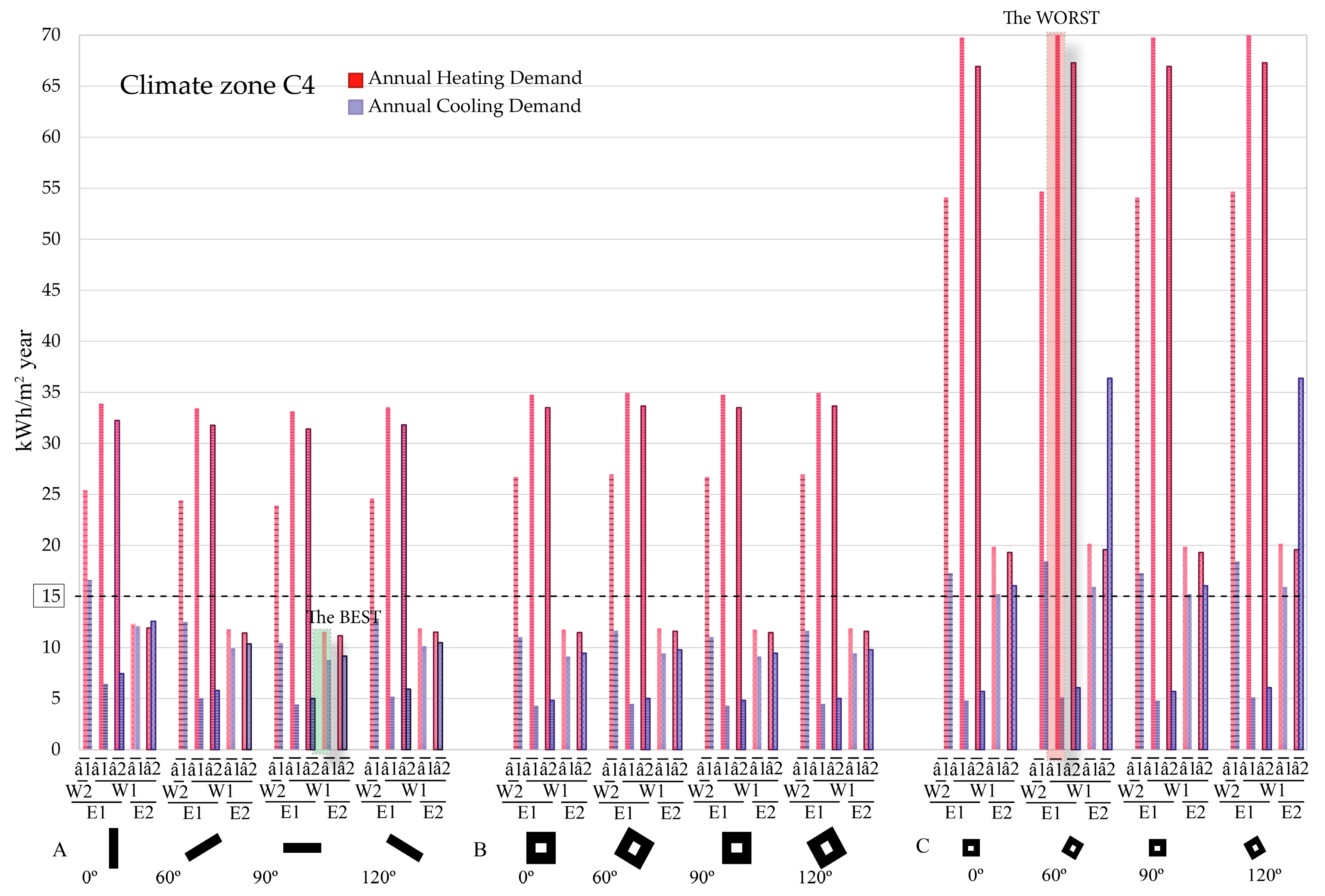
3.4. Climate Zone C4
Figure 6 shows the analysis of the results pertaining to climate zone C4. The best model within zone C4 is the same as those obtained within climate zones A4 and B4. The lowest heating energy demand (Q-heat = 11.16 kWhm
−2) is associated to model A when rotated 90° and using envelope E2 (U = 0.35 Wm
−2K
−1), as well as a WWR equal to W1 (20%), dark colors â
2 (0.2), and a lower shape factor (0.26). The lowest cooling energy demand (Q-cool = 4.3 kWhm
−2) is associated to model B when rotated 0° and 90° and using envelope E1 (U = 1.58 Wm
−2K
−1), as well as a WWR equal to W1 (20%), light colors â
1 (0.64), and a lower shape factor (0.26).
Considering the heating energy demand, the worst model coincides with that of climate zone B4 (Q-heat = 70.11 kWhm−2). It corresponds to the highest heating energy demand associated to model C when rotated 60° and using envelope E1 (U = 1.58 Wm−2K−1), as well as a WWR equal to W1 (20%), light colors â1 (0.64), and a greater shape factor (0.48) (i.e., C-60°-E1w1â1). As for the cooling energy demand, it coincides with the worst model pertaining to climate zones A4 and B4. The highest cooling energy demand (Q-cool = 18.43 kWhm−2) is associated to model C when rotated 60° and 120° and using envelope E1 (U = 1.58 Wm−2K–1), as well as a WWR equal to W2 (40%), light colors â1 (0.64), and a greater shape factor (0.48) (i.e., C-60° and 120°-E1w2â1).
As for the total energy demand (Q), the optimal model coincides with those of climate zones A4 and B4. This configuration is given by model A (Q = 20.33 kWhm−2) when rotated 90° and using envelope E2 (U = 0.35 Wm–2K–1), as well as a WWR equal to W1 (20%), light colors â1 (0.64), and a lower shape factor (0.26) (i.e., A-90°-E2w1â1). However, the worst model in terms of the total energy demand within this climate zone C4 does not coincide with those of the remaining climate zones. The highest value of the total energy demand corresponds to model C (75.23 kWhm−2) when rotated 60° and using envelope E1 (U = 1.58 Wm−2K−1), as well as a WWR equal to W1 (20%), light colors â1 (0.64), and a greater shape factor (0.48). (i.e., C-60°-E1w1â1). Therefore, the worst model with regard to the total energy demand does not correspond to the worst one relevant to the cooling energy demand. This difference lies in the WWR. In fact, the worst model corresponds to a lower WWR (20%) whereas the worst model when considering climate zones A4 and B4 corresponds to a greater WWR (0.48).
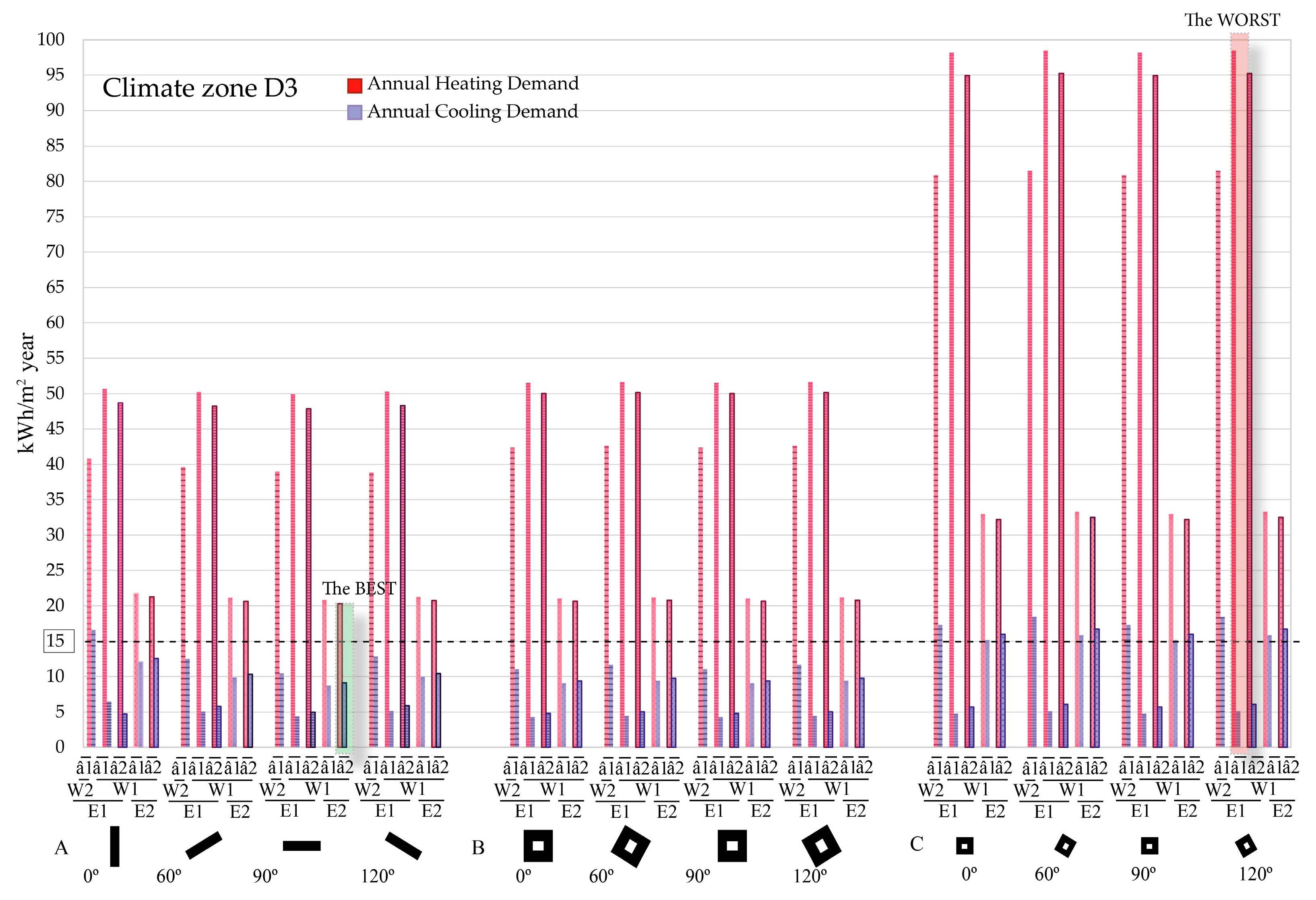
3.5. Climate Zone D3
Figure 7 shows the analysis of the results pertaining to climate zone D3. The lowest heating energy demand within zone E1 is the same as those obtained within climate zones A4, B4, and C4. It corresponds to model A when rotated 90° and using envelope E2 (U = 0.35 Wm
−2K
−1), as well as a WWR equal to W1 (20%), dark colors â
1 (0.64), and a lower shape factor (0.26). This corresponds to the model A-90°-E2w1â
2 with a value of the heating energy demand equal to 20.29 kWhm
−2. However, the lowest cooling energy demand within zone D3 corresponds to model B (Q-cool=4.29 kWhm
−2) when rotated 0° and 90° and using envelope E1 (U = 1.58 Wm
−2K
−1), as well as a WWR equal to W1 (20%), light colors â1 (0.64), and a lower shape factor (0.26), i.e., B-0º and 90º-E1w1â1.
The highest heating energy demand within zone D3 is the same as that of climate zone A4. This model corresponds to a greater value of the heating energy demand associated to model C (Q-heat=98.51 kWhm−2) when rotated 120º and using envelope E1 (U = 1.58 Wm−2K−1), as well as a WWR equal to W1 (20%), light colors â1 (0.64), and a greater shape factor (0.48) (i.e., C-120°-E1w1â1). The highest cooling energy demand (Q-cool = 18.44 kWhm−2) coincides with those of climate zones A4, B4, and C4. In this case it corresponds to a greater value of the cooling energy demand associated to model C when rotated 60° and 120° and using envelope E1 (U = 1.58 Wm−2K−1), as well as a WWR equal to W2 (40%), light colors â1 (0.64), and a greater shape factor (0.48) (i.e., C-60° and 120°-E1w2â1).
With regard to the total energy demand (Q), the best model is different from those of the climate zones previously considered. In this particular case, such best model corresponds to model A (Q = 29.41 kWhm−2) when rotated 90° and using envelope E2 (U = 0.35 Wm−2K−1), as well as a WWR equal to W1 (20%), dark colors â2 (0.2), and a lower shape factor (0.26). For the first time the use of dark colors results in a reduction of the overall consumption. On the other hand, the worst model does not coincide with the one defined for zone C4. In this particular case, it corresponds to model C (Q=103.63 kWhm−2) when rotated 120° and using envelope E1 (U = 1.58 Wm−2K−1), as well as a WWR equal to W1 (20%), light colors â1 (0.64), and a greater shape factor (0.48) (C-120°-E1w1â1). The orientation in this case is 120° whereas that of zone C4 is 60°.
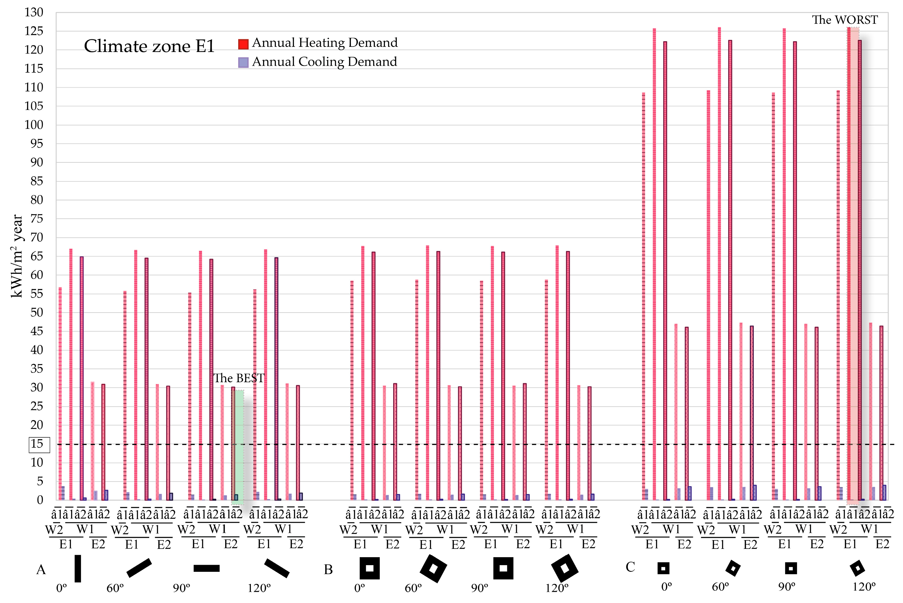
3.6. Climate Zone E1
Figure 8 shows the analysis of the results pertaining to climate zone E1. The lowest heating energy demand within zone E1 is the same as those obtained within all the climate zones previously considered. It corresponds to model A-90°-E2w1â
2 with a value of heating energy demand equal to 30.14 kWhm
−2. However, the lowest cooling energy demand within zone E1 corresponds to model C (Q-cool = 0.14 kWhm
−2) when rotated 90° and using envelope E1 (U = 1.58 Wm
−2K
−1), as well as a WWR equal to W1 (20%), light colors â
1 (0.64), and a greater shape factor (0.48).
The highest heating energy demand within zone E1 is the same as that of climate zone D3. This worst model corresponds to the highest heating energy demand associated to model C (Q-heat=126.04 kWhm−2) when rotated 120° using envelope E1 (U = 1.58 Wm−2K−1), as well as a WWR equal to W1 (20%), light colors â1 (0.64), and a greater shape factor (0.48). The worst model in terms of the cooling energy demand (Q-cool = 4.01 kWhm−2) is different from the rest of the zones analyzed previously. In this case it corresponds to the highest cooling energy demand associated to model C when rotated 120° and using envelope E2 (U = 0.35 Wm−2K−1), as well as a WWR equal to W1(20%), dark colors â2 (0.8), and a greater shape factor (0.48). The parameter varied is the transmittance of the wall E2 (U = 0.35 Wm−2K−1). In the previous climate zones, it corresponds to the value E1 (U = 1.58 Wm−2K−1).
The lowest total energy demand within zone E1 is the same as that of zone D3. The best model corresponds to model A (Q = 31.67 kWhm−2) when rotated 90° and using envelope E2 (U = 0.35 Wm−2K−1), as well as a WWR equal to W1 (20%), dark colors â2 (0.2), and a lower shape factor (0.26). On the other hand, the highest total energy demand is that of zone D3. In this particular case it corresponds to the highest total energy demand associated to model C (Q = 126.19 kWhm−2) when rotated 120° using envelope E1 (U = 1.58 Wm−2K−1), as well as a WWR equal to W1 (20%), light colors â1 (0.64), and a greater shape factor (0.46). Both models are similar to that of climate zone D3.
3.7. Climates Cross-Comparison
Table 6 shows the comparison between the optimal models and the worst ones with respect to the different climate zones. The results show how building A, which corresponds to a linear block, is the optimal shape with regard to the heating energy demand and the total energy demand. They also indicate that model C, which is the one with the greatest shape factor (0.48), presents the highest energy demand values. Heating in Spain is the main responsible for energy consumption. In colder climates such as E1, the amount of heat loss through the envelope is greater than the amount of heat that can be gained when increasing the external surface receiving solar radiation. Therefore, a proportionality is established between the increment of the shape factor (i.e., with a lower index of compactness) and the increment of the energy needed for heating [
57]. Accordingly, this research work shows that the optimal model is that with the lowest shape factor.
As for the orientation, the North-South orientation (0° and 90°) of the main façades is the best one. The design of buildings oriented to the North-South axis is recommended, with the largest façade oriented to the south. Orientation is one of the parameters that has the most impact on the design of buildings. Most books, guides or manuals on passive solar techniques recommend a southerly orientation, although consensus is based on the fact that the best option is an orientation of 20–30° to the south [
58]. This has to do with the fact that the southern side of a building receives the maximum amount of solar radiation whereas the northern side receives the minimum amount of solar radiation (i.e., just its diffuse component).
Accordingly, in the current research, the optimal orientation found in the five climate zones for models A, B and C is 90° (North-South), the best model being A while the worst being C.
As for the thermal transmittance of the external walls, the best configuration is that complying with the SBTC (0.35 Wm−2K−1) and showing the lowest WWR (20%). In terms of solar reflectance, it is found that in climate zones A4, B4, and C4 the use of light colors is better, whereas in climate zones D3 and E1 the best option is using darker colors.
On the other hand, the worst configuration is found for the C-60° and 120° from the North model, with walls U-value not complying with the SBTC prescriptions (1.58 Wm−2K−1). Regarding the WWR, in zones A4 and B4 the use of larger WWR’s is unfavorable, while the use of lower WWR is unfavorable when considering zones C4, D3, and E1. With respect to solar reflectance, it is pointed out that the worst case is given by the use of light colors in all climates.
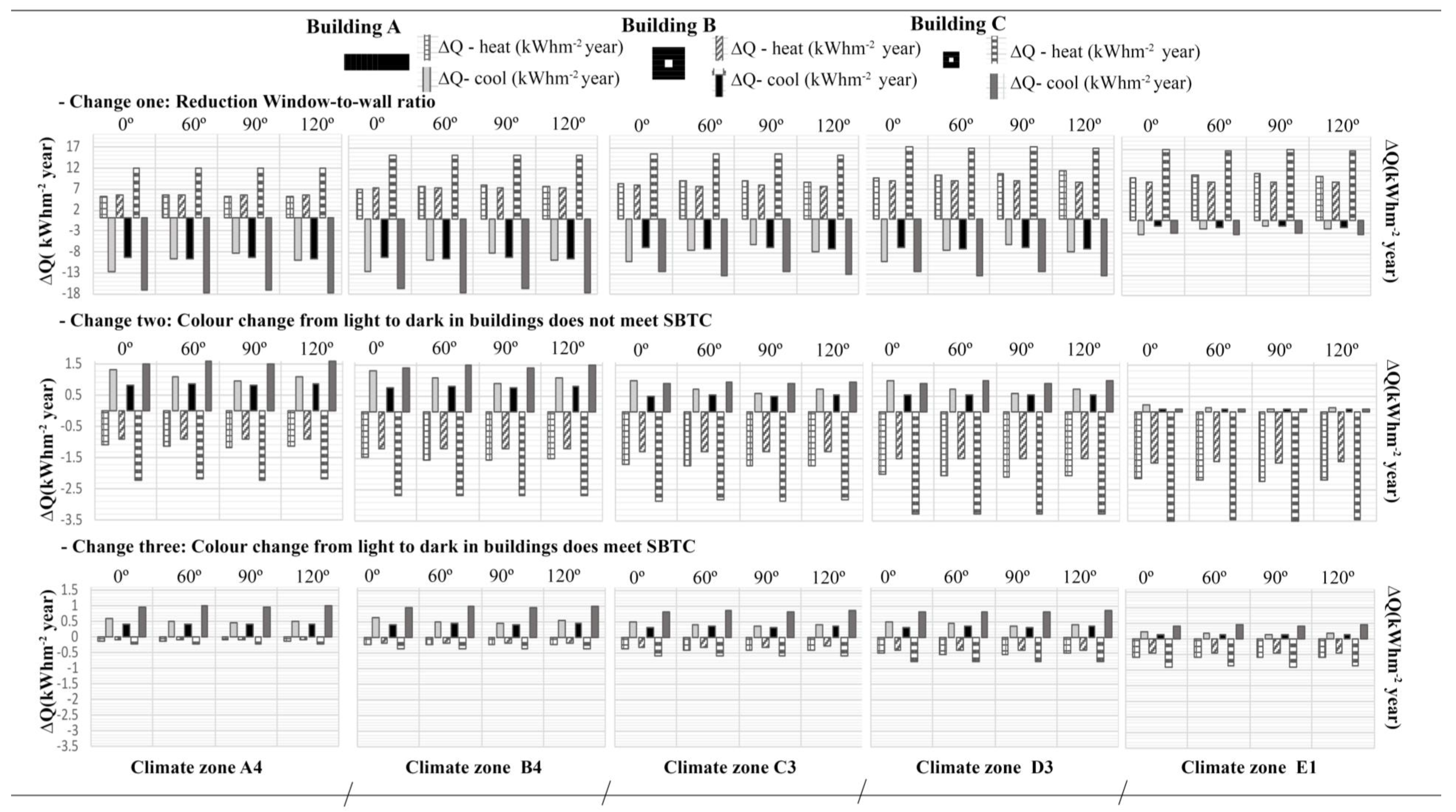
3.8. Sensitivity Analysis of the Most Important Parameters
This section comments the results of a sensitivity analysis carried out on the parameters architects and design professionals should particularly take care of as they mostly affect the energy needs of the buildings: WWR, solar reflectance and U-values of the external walls.
Figure 9 analyzes the variations of these parameters according to all the climate zones, with positive values expressing an increase and negative values indicating reductions.
The graphic is divided into three parts; each of them corresponds to a specific variation in the architectural design. The first variation corresponds to the reduction of the WWR from 40% to 20%, and is depicted in the top row.
The second one is the variation from light to darker color when the thermal transmittance of the envelope meets SBTC prescriptions. The base model has a value of â1 equal to 0.64, while the final model has a value â2 equal to 0.2. The third variation is that from a light color to a darker one when the thermal transmittance does not comply with SBTC.
Figure 9 shows that, when the WWR is reduced (top row), the heating energy demand gets increased. The increments obtained in the different climates are of 6.91 kWhm
−2 for climate zone A4, 8.29 kWhm
−2 for climate zone B4, 7.73 kWhm
−2 for zone C4, 8.35 kWhm
−2 for zone D3 and 8.02 kWhm
−2 for climate zone E1.
The second variation (i.e., middle row) corresponds to the shift from light to dark colors when the thermal transmittance of the envelope does not meet the SBTC requirements. It is found that in such particular case the cooling energy demand increases as following: in climate A4 of 0.78 kWhm−2, in climate B4 of 0.73 kWhm−2, in climate C4 the increase is of 0.47 kWhm−2, while for climates D3 and E1 they amount to 0.46 kWhm−2 and 0.14 kWhm−2 respectively. On the other hand, it can be noted that the heating energy demand gets reduced in a range of 1.3 kWhm−2 for climate zone A4 to 1.88 kWhm−2 for climate zone E1.
Finally, the third variation corresponds to a shift from light to dark colors when the thermal transmittance does not comply with the SBTC requirements. It is found that the heating demand gets reduced of the following amount: 0.59 kWhm−2 in climate zone A4, 0.58 kWhm−2 in climate zone B4, 0.53 kWhm−2 in climate zone C4, 0.52 kWhm−2 in climate zone D3 and 0.31 kWhm−2 in climate zone E1. On the other hand, the cooling energy demand increases in a range of 0.12 kWhm−2 for climate zone A4 to 0.45kWhm−2 for climate zone E1.
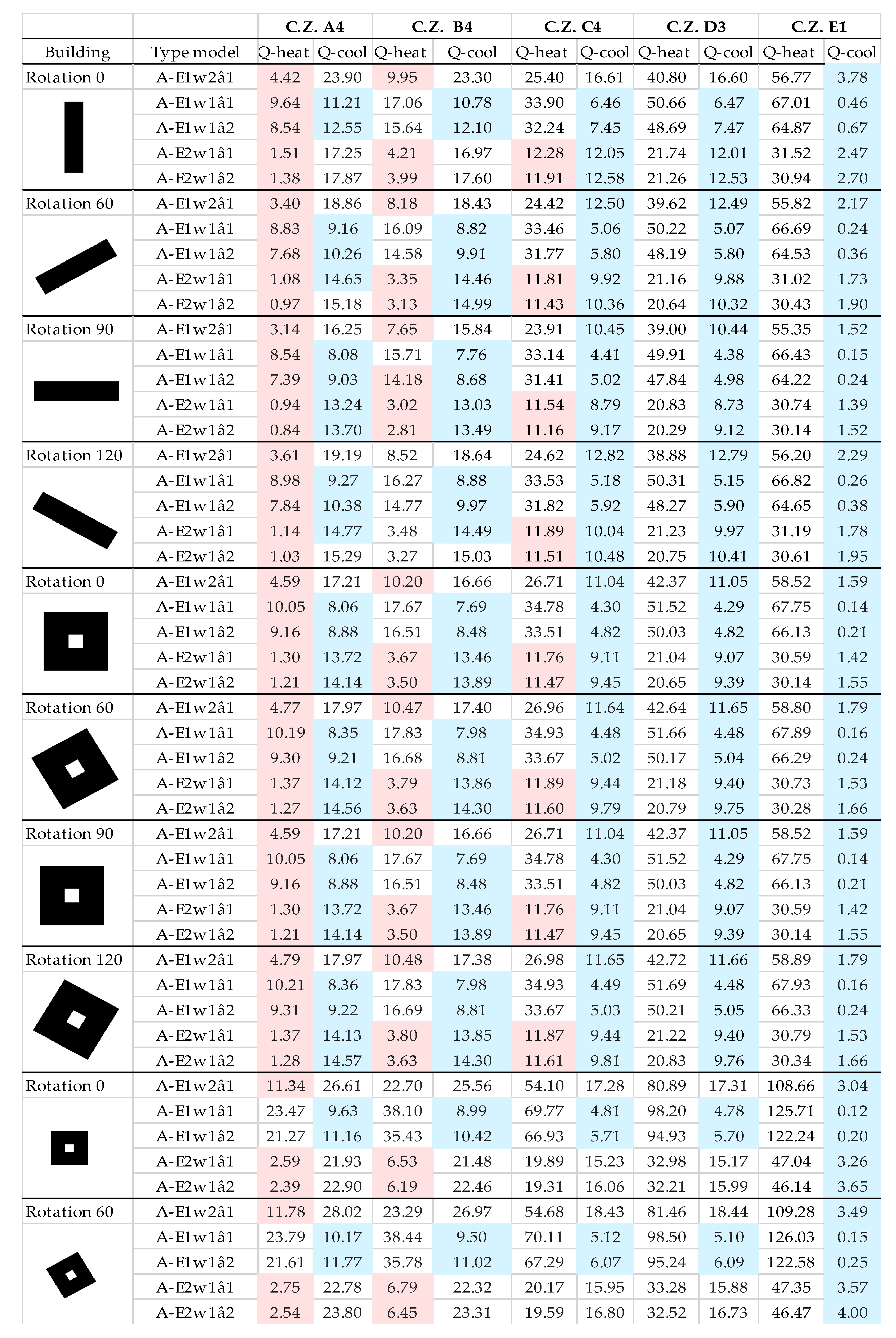
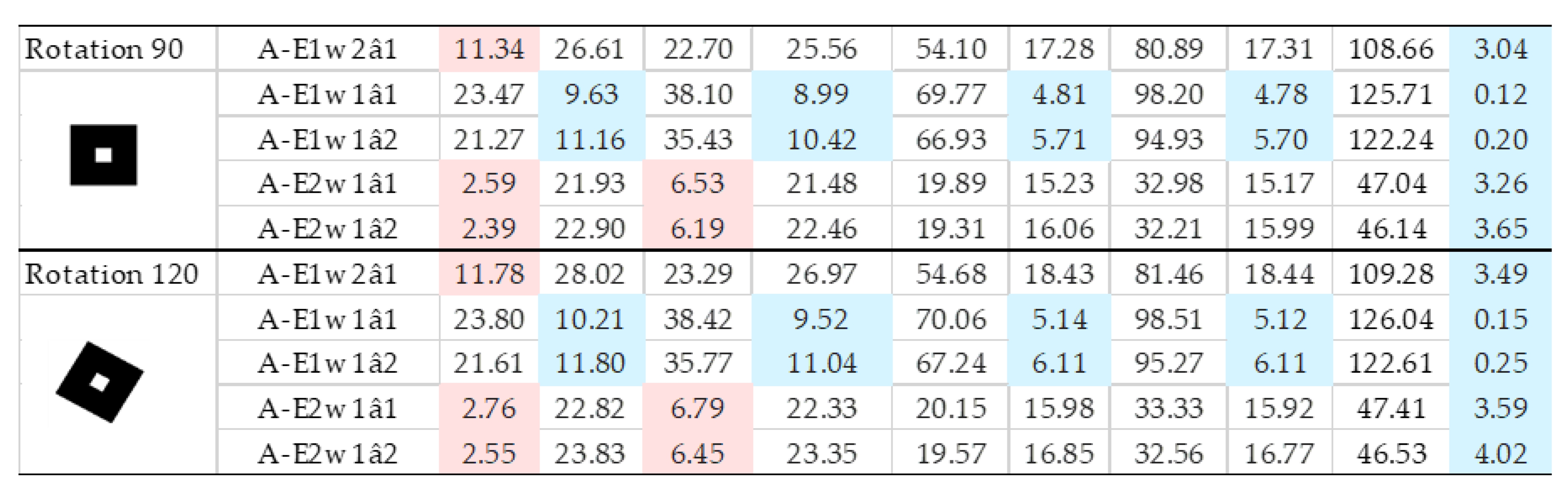
4. Compliance with the PH Standard
This section deals with the compliance of the simulated models with the PH threshold of 15kWhm
−2 for heating and cooling purposes. Red values shown in
Figure 10 correspond to the heating values that are lower than the PH standard, while the blue values correspond to the cooling values meeting the PH standard.
The first conclusion that can be drawn is that buildings located in climate zones C4, D3, and E1 deserve more detailed studies since their design according to basic passive design measures does not allow meet the PH standard requirements. Looking closer, models A and B that present a shape factor of 0.26 generally meet the PH criterion when considering climate zones A4 and B4. On the contrary, model C does not meet the standards in such climates.
When the heating energy demand column is analyzed, it can be noted that in climate zones A4 and B4 most of the demand is below 15 kWhm−2. On the other hand, as long as climate zones become more severe during the winter (i.e., climate zones D3 and E1), the heating energy demand is never below 15 kWhm−2. If the shape factor is considered, models A and B (i.e., those models with a shape factor of 0.26) do meet the PH standard, whereas the heating demand pertaining to model C is seldom below 15 kWhm−2.
As for the cooling energy demand column, the opposite results are obtained. It is observed that in climate zones E1 and D3 most of the cooling demand is below 15 kWhm
−2. On the other hand, as long as climate zones become more severe during the summer (i.e., climate zones A4 and B4), only few models present demand values below 15 kWhm
−2. As far as the shape factor is concerned, the same behavior described above is found. Models A and B do meet the PH standard, whereas if considering model C the cooling demand is seldom below 15 kWhm
−2. According to
Figure 10, in climate zones such as those of Spain, heating must be the main focus with regard to the design of buildings in order to comply with the PH standard.
5. Conclusions
This research work is intended to support building designers and professionals during the early design stages of residential buildings located in Spain by providing an energy analysis of different architectural strategies typically implemented in passive design.
Three building types representative of the multi-dwelling units (MDUs) stock are simulated through a parametric analysis in Design Builder. For each typology, parameters such as orientation, Window-to-Wall Ratio (WWR), shape factor, outer walls construction, color of the envelope, and climate zones are evaluated, resulting in 300 simulations. Such parameters have been graphed and related with the building design, so that the energy demand for space heating and cooling can be directly related with the specific design parameters, and the communication gap between simulation outputs and architects’ understanding of them closed.
Regarding the heating demand, the best model turns out to be A-90°-E2w1â2 for all climates. It is defined by using the thermal transmittance that meets the SCTB (U = 0.35 Wm−2K−1), as well as a low WWR (20%) along with dark colors (â2 = 0.2). Regarding the worst model, it is found to be the C-60° and 120° from the North when using a thermal transmittance that does not comply with the SCTB (U = 1.58 Wm−2K−1), as well as the lowest percentage of WWR (20%) and light colors (â1 = 0.64).
Regarding the cooling demand, the best model is not the same in all climate zones. In zones A4, B4, C4, and D3, it is B-0° oriented 90° from the North when using a thermal transmittance that does not comply with the SCTB as well as the lowest percentage of WWR (20%) and light colors (E1w1â1). As for the E1 climate zone, the best configuration is found when using external walls whose thermal transmittance does not comply with the SCTB (U = 1.58 Wm−2K−1), having a low value of the WWR parameter (20%) and light colors for finishing (â1 = 0.64). Regarding the worst model, it always turns out to be the same one in all climate zones, i.e. C—60° and 120° from the North-E1w2â1. In such cases the thermal transmittance does not comply with the SCTB (U = 1.58 Wm−2K−1), the greatest percentage of WWR (40%) is used and the colors considered are light (â1 = 0.64).
Regarding the total energy demand, the best model in climate zones A4, B4, and C4 is A-90°-E2w1â1. It is defined using the thermal transmittance that meets the SCTB (U= 0.35 Wm−2K−1), as well as the lowest percentage of WWR (W1 = 20%) when using light colors (â1 = 0.64). On the contrary, the best model in climate zones D3 and E1 is A-90°-E2w1â2. It is defined using the thermal transmittance that meets the SCTB (U = 0.35 Wm−2K−1), as well as the lowest percentage of WWR (W1 = 20%) when using dark colors (â2 = 0.2). Regarding the worst model in climate zones A4 and B4, it happens to be the C-60° and 120° ones when using the thermal transmittance of the wall that does not comply with the SCTB (U = 1.58 Wm−2K−1), as well as the lowest percentage of WWR (20%) when using light colors (â1 = 0.64). Regarding climate zones C4, the worst model is C-60°-E1w1â1. It is defined using the thermal transmittance that does not comply with the SCTB (U = 1.58 Wm−2K−1), as well as the lowest percentage of WWR (W1 = 20%) when using light colors (â1 = 0.64). As for climate zones D3 and E1, the worst model is C-120°-E1w1â1. It is defined using the thermal transmittance that does not comply with the SCTB (U = 1.58 Wm−2K−1), as well as the lowest percentage of WWR (W1=20%) when using light colors (â1 = 0.64).
Most parameters produce contradictory effects when comparing the heating and cooling demands. As for the shape factor, if considering square building the heating energy demand reaches its minimum value when the façades are oriented directly to the four cardinal points. In a rectangular building, the heating demand is reduced as the façade facing east is smaller. The reduction of the WWR causes the heating demand to decrease and the cooling demand to increase; this is beneficial for climate zone E1 but harmful for A4. In addition, the reduction in the WWR when considering A4 climates helps the users to reduce the cooling energy demand while the same action in cooler areas worsens the heating energy demand.
Regarding the reflectance of the materials, in climate zone A4 the use of reflective and selective cold materials is beneficial. When considering E1 (U = 1.58 Wm−2K−1), the use of absorptive materials is definitely recommended. In cooler zones such as E1, it is instead recommended to use darker colors while in warmer zones such as A4 it is recommended to use lighter colors (â1 = 0.64).
Finally, those buildings located in climate zones C4, D3, and E1 require more detailed analysis since their design does not meet the PH standard according to the basic passive design measures discussed. It was demonstrated the importance to applying the passive house principles in early design phases in order to reduce energy consumptions. The adoption of useful tool like dynamic simulations software can help architects, designs, builders and stakeholders in the decision—making process to recognize that the PH model is one of the most effective ways of reducing carbon emissions.
More efficient designs can be obtained by using appropriate passive strategies which will be accomplished by building designers committed and aware of the current situation in order to comply with the requirements of European energy policies. Although considering the users’ habits is still a pending issue, using passive strategies is definitely a breakthrough in the design of efficient buildings.

 ,
, 


