Modeling of Heat Transfer Coefficient in Solar Greenhouse Type Drying Systems

Abstract

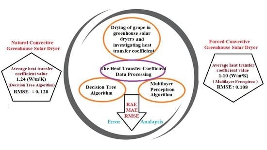
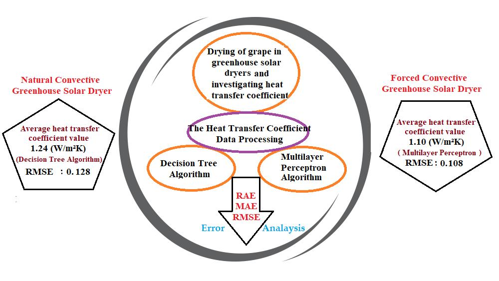
As a sustainable energy source, solar energy is used in many applications. A greenhouse type dryer, which is a food drying system, directly benefits from solar energy. Convective heat transfer coefficient (h_c) is an important parameter in food drying systems, in terms of system design and performance. Many parameters and equations are used to determine h_c. However, as it is difficult to manually process and analyze large amounts of data and different formulations, machine learning algorithms are preferred. In this study, natural and forced convective solar greenhouse type dryers were designed. In a solar greenhouse type dryer, grape is dried in natural (GDNC) and forced convection (GDFC). For convective heat transfer coefficient (h_c), predictive models were created using a multilayer perceptron (MLP)—which has many uses in drying applications, as mentioned in the literature—and decision tree (DT), which has not been used before in food drying applications. The machine learning algorithms and results of the estimated models are compared in this study. Error analyses were performed to determine the accuracy rates of the obtained models. As a result, the h_c value of the dried grape product in a natural convective solar greenhouse type dryer was 11.3% higher than that of the forced type. The DT algorithm was found to be a more successful model than the MLP algorithm in estimating hc values in HDFC according to Root Mean Square Error. (RMSE = 0.0903). On the contrary, the MLP algorithm was more successful than the DT algorithm in estimating h_c values in GDNC (RMSE = 0.0815).

1. Introduction

The short wavelengths emitted by the sun’s radiant energy are absorbed through permeable air and reflect on the earth’s surface as infrared radiation. These rays are then absorbed by atmospheric gases, such as carbon dioxide, methane, nitrous oxide, and water vapor. Infrared rays that are held by atmospheric gases increase the temperature of the earth’s surface, an event known as the greenhouse effect [1,2,3].

The use of solar energy, a renewable energy source, has great potential and plays a central role in ensuring and increasing sustainability, which, in turn, is the key to making current energy scenarios more environmentally friendly for future generations. Thus, systems that use solar energy, such as greenhouses, are gaining importance [4,5,6,7,8]. Greenhouse systems are closed structures with a transparent cover that enable short wavelengths of solar radiation to pass through. These systems offer microclimate conditions by keeping the infrared rays in the environment [9,10,11]. A greenhouse dryer reduces drying time by controlling temperature and relative humidity. Due to this advantage, it is a suitable option for drying applications [12,13]. The location, shape, size, and design of the greenhouse is of great importance when building a system specific to the product to be dried [2,13,14]. This process includes heat and mass transfer events. Heat energy is provided in two steps: The first is sensible heat, which occurs when the product’s temperature increases. The second is the formation of latent heat from the product, vaporized by moisture [7,15]. One of the most widely used classification methods for thermal modelling of greenhouse drying systems is the air circulation method in the drying chamber [11,16]. These systems are classified in two different ways, prior to air circulation: The first is natural convection greenhouse dryers, in which solar radiation passes through the transparent cover to heat the product and increase its temperature. Heat transfer in natural convection greenhouses is based on the principle of thermophysical effects [17,18,19]. The second greenhouse is a forced convection greenhouse dryer, which allows humid air to be removed from the product in the greenhouse using a fan or a blower. Optimum air flow can be provided with the help of a fan used in forced convection greenhouse drying systems [20,21,22].

There are many modelling studies in the literature for greenhouse dryers. Kumar and Tiwari [23] dried jaggery in a natural convection greenhouse drying system and modelled the system thermally. With the created model, they tried to estimate the temperature of the dried product, air temperature of the greenhouse, amount of vaporized moisture, and thermal performance of the greenhouse depending on the intensity of the radiation and the ambient temperature; and validated the results obtained with the experimental results. They found that the obtained model offered good results. Prakash and Kumar [24] created an Adaptive Neural Fuzzy Inference System (ANFIS) model, which is a neural fuzzy system, to estimate product temperature, greenhouse air temperature, and amount of vaporized moisture during the drying of the same product in a natural convection greenhouse drying system. In order to ascertain the suitability of the model, they obtained its validity and observed that the ANFIS model predicted different drying parameters for the experimentally dried jaggery product. Condori and Saravia [22] carried out an analytical study on the moisture ratio of red pepper dried in greenhouse dryers with two different types of forced convections. The simulation tests showed that the use of a double drying chamber for red pepper increased drying efficiency by almost 90%. Jain and Jain [25] provided a transient analytical model for a dryer. As a result of their study, the humidity in the air and the drying rate of the product increased with increase in depth of the dryer bed. Bala et al. [26] studied a solar-assisted tunnel dryer for pineapple slices in Bangladesh’s climate conditions. The researchers found that the pineapple slices dried with the designed solar tunnel type dryer were protected from external factors, such as rain, insects, and dust, and thus, dried products of a higher quality were obtained, as compared to those dried under the sun.

Drying is a heat-based and mass transfer process. Therefore, in order to determine the optimum drying air conditions in the design of drying systems, a drying rate should be modeled. While designing drying systems, the convective heat transfer coefficient value (h_c) has a significant effect on the drying rate, due to the temperature difference between the product and air. Therefore, the effect of convective heat transfer coefficient value on the simulation of drying rate is quite important [27]. Akpinar [28] examined the variation of convective heat transfer coefficient prior to different air velocities and temperatures using a variety of products in a convective dryer. It was observed that there was an increase in the convective heat transfer coefficient with the rise of drying air velocity. However, it was also observed that there was no similar increase in the convective heat transfer coefficient with the increase of drying air temperature. Akpinar [29] used data obtained from open sun-drying experiments to determine the convective heat transfer coefficient values of food products. At the end of this study, C and n constants were calculated in terms of experimental data of eight different products. The researcher then obtained h_c values for eight different products and stated that these values varied from 1.136 to 11.323 W/m²°C. Goyal and Tiwari [30] carried out a heat and mass transfer in a drying system. They estimated convective heat transfer coefficient values using simple and multiple regression techniques, and established a relationship between heat and mass transfer using the C, m, and n values of the dried products.

Several predictive models have been developed in the literature for estimating the convective heat transfer coefficient [31]. Artificial neural networks are frequently used in the creation of these models [32,33,34,35]. Another classification and estimated model method using regression is decision trees [36]. Decision trees are not a single formula covering all data. They are local models. In the case of data with a lot of features, it is very hard to correctly fit data into a single model. Decision trees divide a dataset into two or more subsets until they reach the stop criterion [37]. Alonso et al. performed a study on the estimation of the environmental and agricultural impacts of sewage sludge on fertilization using decision trees. The results proved that decision trees interpret predictions for complex data in medium and long periods of agricultural experience [37].

In this study, natural (GDNC) and forced (GDFC) convection coefficients of the drying of grape grains in a greenhouse dryer were experimentally determined. Then, the experimentally calculated h_c values were estimated to be of high accuracy using different types of machine algorithms. In order to estimate h_c values, machine algorithms such as Multilayer Perceptron (MLP) and Decision Tree (DT) were used. In literature, the use of an MLP model to estimate other drying kinetics is available. However, the use of MLP and DT models to estimate convective heat transfer coefficients obtained experimentally from food drying processes has not been found in open literature. Therefore, our study, which is based on the modeling of a convective heat transfer coefficient with DT and MLP in drying systems, is expected to be a case study for many researchers.

2. Materials and Methods

In this study, heat transfer coefficients were calculated for grapes at different types of greenhouse solar dryers. For predicted heat transfer coefficients, a predictive model was developed by using DT and MLP.

3.1. Experimental Setup

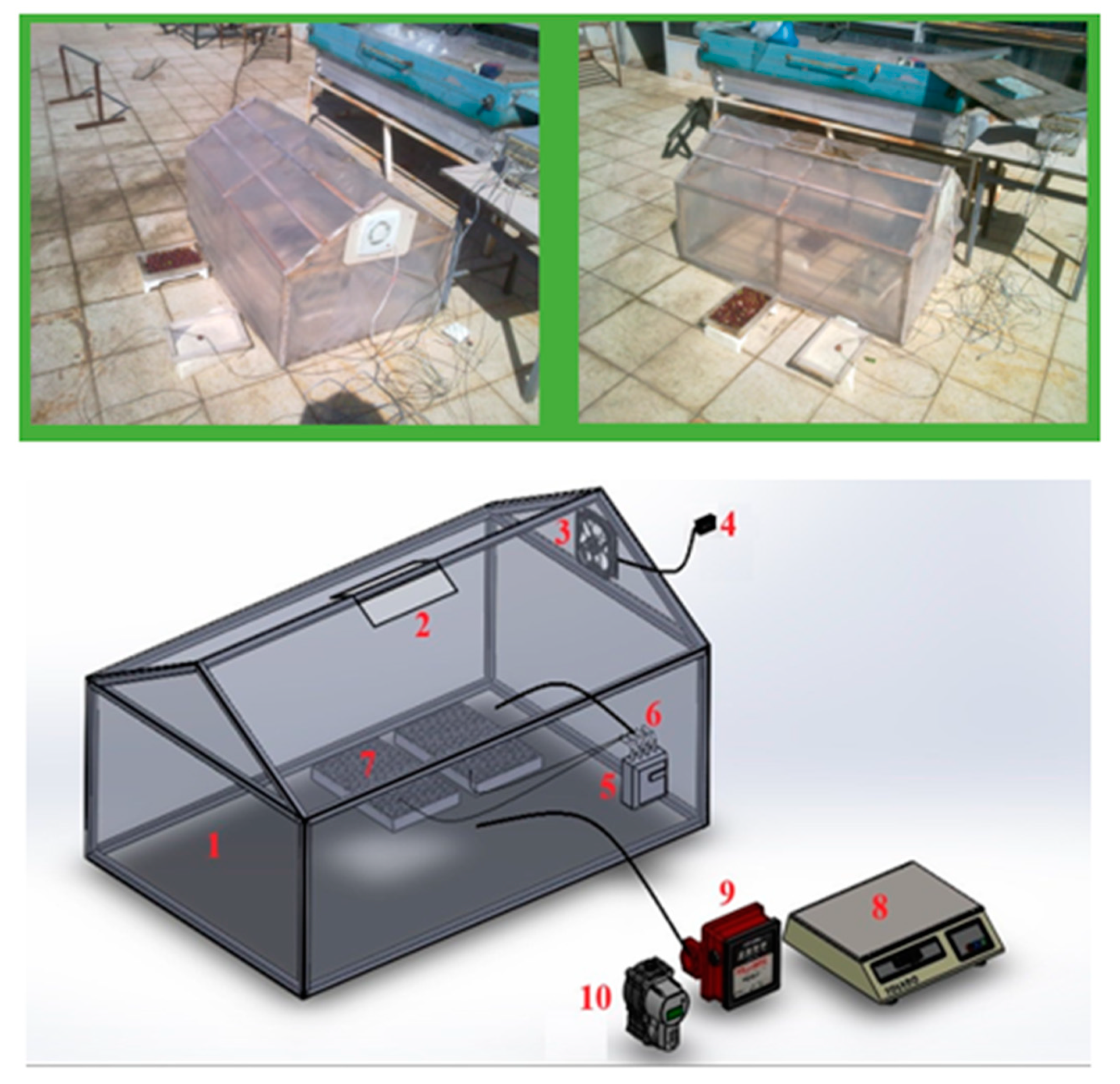
A greenhouse type dryer was designed and manufactured for the drying of grapes in Elazığ province, Turkey. The dryer was built on a concrete floor and covered with a nylon sheet. For sizing, the dimensions of a greenhouse dryer manufactured before us were used [23,38]. The greenhouse type dryer was made of 1.20 × 0.78 m² area with a roof scaffold and transparent plastic material. The length of the center and the walls are approximately 0.60 m and 0.40 m, respectively. The experiments were carried out in a greenhouse for forced convection (GDFC) and a greenhouse for natural convection drying (GDNC). An air gap of 0.0722 m² was formed on the roof of the GDNC. Thus, the moisture in the product was removed by the thermophysical effects caused by the air gap. In the forced drying process, a fan with air speed of 2.4 m/s was mounted on the side wall to remove moisture from the product. The air gap was closed for forced drying. Grape was selected as the product to be dried. The long drying duration for grape under the sun is mentioned in the literature [39]. However, a huge amount of data is required when modeling with the help of a machine-learning algorithm. The reason for this is because the model has a lower error rate, owing to the increasing number of data. Grapes were selected due to the long time it takes to dry. Thus, more data were obtained and a more successful model was formed.

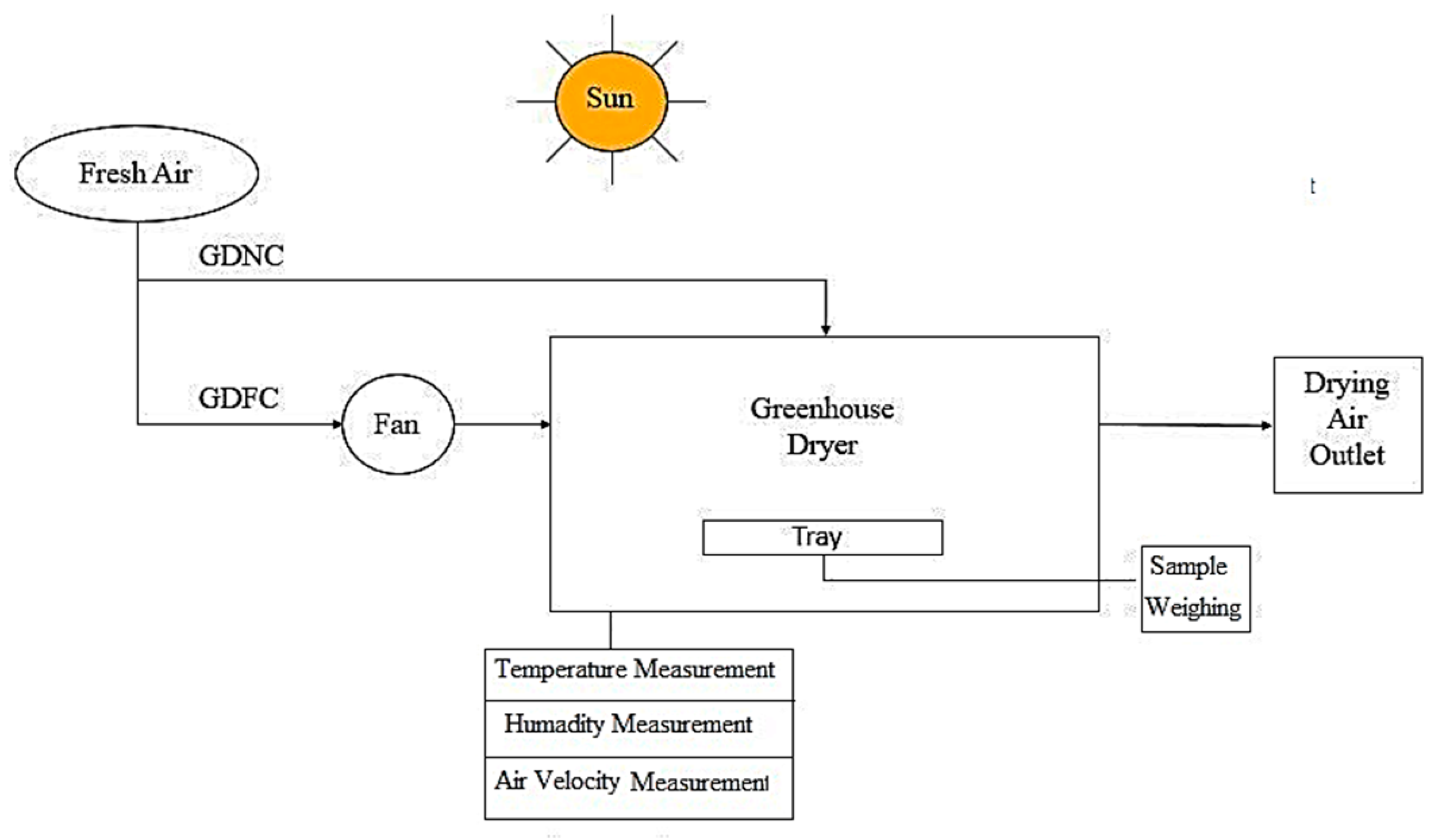
Air was allowed to enter the greenhouse from the side of the drying chamber and the products were paced on a mesh tray. During the experiments, the greenhouse was positioned in the East-West direction in order to ensure distribution of radiation [6,11,26]. Figure 1 shows the sections of the greenhouse solar dryer designed for drying in GDFC and GDNC. Figure 2 shows a diagram of the drying process. In addition, the devices used for measurement and error values are given in

Table 1. Devices used in measurements and error values.

Measurement Parameter	Brand	Accuracy
Temperature	20 Channels Elimko 6400	0.1 °C
Air Velocity	LUTRON 4201 0.4–30 m/s	±2%
Relative humidity	EXTECH 444,731 Thermo-hygrometer	±1%
Weight	BEL (maks 2000 gr)	0.01 gr
Radiation	Kipp-Zonen pyranometer and CC12 model digital solar integrator	±0.1 Wm−2

.

The uncertainty value of the measurements taken in the experiment set was based on a method by Kline and McClintock (Equation (1)) [40,41]. In Equation (2), x represents uncertainty properties and W represents uncertainty value. In this study, the uncertainty analysis calculated for various measurements is shown in

Table 2. Uncertainty analysis results.

Parameters	Uncertainty Value (%)
Uncertainty in surface temperature measurements	±0.583
Uncertainty in greenhouse air temperature measurements	±0.386
Uncertainty in humidity measurements	±0.1
Uncertainty in solar radiation measurements	±0.506
Uncertainty in weight measurements	±0.5
Uncertainty in air velocity measurements	±0.14

:

$${\mathrm{W}}_{\mathrm{x}}={\left[{(x_1)}^2+{(x_2)}^2+{(x_3)}^2+\cdots +{(x_{\infty })}^2\right]}^{1/2}$$

(1)

3.2. Calculation Procedure

The convective heat transfer coefficient (h_c) is determined by Nusselt number [42,43]:

$${\mathrm{h}}_{\mathrm{c}}=\frac{Nu·{\mathrm{K}}_{\mathrm{v}}}{\mathrm{X}}$$

(2)

where, $h_c$ is convective heat transfer coefficient (W/m²°C), $K_v$ is thermal conductivity for humid air (W/m°C), $\mathrm{X}$ is characteristic dimension (m). Convective heat transfer coefficient for natural convection [42,43]:

$$h_c=\frac{K_v}{X}·C·{\left(Gr·Pr\right)}^n$$

(3)

for forced convection:

$$h_c=\frac{K_v}{X}·C·{\left(Re·Pr\right)}^n$$

(4)

calculated using parameters. Where, C and n are constants, Gr is Grashof number, Pr is Prandtl number, Re is Reynolds number.

The amount of heat required to vaporize moisture is calculated by Equation (5) [38,42,43]:

$${\dot{Q}}_e=0.016·h_c·\left[P\left(T_c\right)-\gamma P\left(T_e\right)\right]$$

(5)

where, ${\dot{Q}}_e$ is the amount of heat required to vaporize moisture (J/m²s), P(T) is partial vapour pressure for any temperature value (N/m²). If the value of h_c in Equations (3) and (4) is written in Equation (5), Equations (6) and (7) are obtained [38,42,43]:

$${\dot{Q}}_e=0.016·\frac{K_v}{X}·C·{\left(Gr·Pr\right)}^n·\left[P\left(T_c\right)-\gamma P\left(T_e\right)\right]$$

(6)

$${\dot{Q}}_e=0.016·\frac{K_v}{X}·C·{\left(Re·Pr\right)}^n·\left[P\left(T_c\right)-\gamma P\left(T_e\right)\right]$$

(7)

Vaporized moisture content is determined by multiplying the amount of heat required for the evaporation of moisture by the time intervals (t) and the tray area (A_t), then divided by the latent heat of evaporation (λ) [38,42,43]:

$$m_{ev}=\frac{{\dot{Q}}_e}{\lambda }·A_t·t=0.016·\frac{K_v}{X·\lambda }·C·{\left(Gr·Pr\right)}^n·\left[P\left(T_c\right)-\gamma P\left(T_e\right)\right]·A_t·t$$

(8)

$$m_{ev}=\frac{{\dot{Q}}_e}{\lambda }·A_t·t=0.016·\frac{K_v}{X·\lambda }·C·{\left(Re·Pr\right)}^n·\left[P\left(T_c\right)-\gamma P\left(T_e\right)\right]·A_t·t$$

(9)

where, $m_{ev}$ is the amount of moisture vaporized (kg). The amount of moisture vaporized ($m_{ev}$) is equal to a constant value, such as Z [38,42,43]:

$$0.016·\frac{K_v}{X·\lambda }·\left[P\left(T_c\right)-\gamma P\left(T_e\right)\right]·A_t·t=Z$$

(10)

In this case, for natural convection:

$$\frac{m_{ev}}{Z}=C·{\left(Gr·Pr\right)}^n$$

(11)

and for forced convection,

$$\frac{m_{ev}}{Z}=C·{\left(Re·Pr\right)}^n$$

(12)

Equations (6) and (7) can be arranged [38,42,43].

If the logarithm of both sides in Equations (11) and (12) is taken, Equations (13) and (14) are obtained [38,42,43]:

$$\ln \left[\frac{m_{ev}}{Z}\right]=\ln C+n\ln \left(GrPr\right)$$

(13)

$$\ln \left[\frac{m_{ev}}{Z}\right]=\ln C+n\ln \left(RePr\right)$$

(14)

Equations (13) and (14) are similar to the equation of a straight line, as given below (Equation (15)):

$$Y=b_1·X+b_0$$

(15)

Here, X and Y are expressed in Equations (16) and (17):

$$Y=\ln \left[\frac{{\dot{m}}_{ev}}{Z}\right],b_1=n, X=\ln \left(GrPr\right), b_0=\ln C$$

(16)

$$Y=\ln \left[\frac{{\dot{m}}_{ev}}{Z}\right], b_1=n, X=\ln \left(RePr\right), b_0=\ln C$$

(17)

Thus, C is expressed as Equation (18):

$$C=e^{b_0}$$

(18)

The convective heat transfer coefficient (h_c) is determined by Nusselt number, which is expressed in terms of Grashof and Prandtl numbers for natural convection and in Reynolds and Prandtl numbers for forced convection. C and n constants, by means of determination of heat transfer coefficient values (h_c), are calculated through linear regression analysis from measured experimental data (product and ambient air temperature, ambient relative humidity and evaporated moisture content values). Then, it is possible to estimate h_c values by obtaining constants C and n.

Different physical properties, density (ρ_v), thermal conductivity (K_v), specific heat (C_v), viscosity (μ_v), and vapor pressure (P) of the moist air are calculated using the following relations [38,42,43]:

$${\rho }_v=\frac{353.44}{\left(T_i+273.15\right)}$$

(19)

$$K_v=0.0244+0.6773\times {10}^{-4}{T}_i$$

(20)

$$C_v=999.2+0.1434T_i+1.101\times {10}^{-4}{T}_i{}^2-6.7581\times {10}^{-8}{T}_i{}^3$$

(21)

$${\mu }_v=1.718\times {10}^{-5}+4.620\times {10}^{-8}{T}_i$$

(22)

$$P\left(T\right)=\exp \left[25.317-\frac{5144}{\left(T_i+273.15\right)}\right]$$

(23)

For the physical properties of moist air, T_i is taken as the average of ambient temperature (T_e) and the center surface temperature (T_c) of the product [38,42,43]:

$$T_i=\frac{\left(T_c+T_e\right)}{2}$$

(24)

Reynolds number (Re), Prandtl number (Pr), and Grashof number (Gr) are obtained by using different physical properties of moist air.

3.3. Machine Learning Algorithms

In recent years, machine learning methods (computational intelligence) have become very popular for different applications. Machine learning is the general name for computer algorithms that can learn structurally and make meaningful predictions on data. These algorithms mainly work by creating models from sample data [44]. Machine learning algorithms are divided into two groups: supervised learning and unsupervised learning. In this study, MLP and DT algorithms, which are machine learning algorithms, are used to estimate the convective heat transfer coefficient. The input and output parameters used in machine estimation algorithms for generating predictive models are given in

Table 3. Input and Output Parameters Used in Estimation Methods.

Input Parameters of Predictive Models
	Unit	Min	Max
Drying time (Min)	Minute	0	1470
Ambient Temperature (Te)	°C	28.5	48.7
Product Temperature (Tc)	°C	23.3	54.4
Evaporated Moisture ($m_{ev}$)	kg	0.0001	0.009
Relative Humidity (γ)	%	5.1	52.2
Reynolds Number (Re)		7382	8023
Prandtl Number (Pr)		0.705	0.706
Radiation (I)	W/m2	296	1015
Output Parameters of Predictive Models
	Unit	Min	Max
Convective Heat Trans. Coeff. (hc)	W/m2°C	0.7703	3.016

.

3.3.1. Multilayer Perceptron (MLP)

The concept of artificial intelligence is a result of long-term studies on computer models of the human brain. The artificial neural network (ANN) technique was subsequently created, and has widespread use due to its reliable results and active role in solving nonlinear problems. In 1960, Widrow and Hoff conducted the first work on a multi-layered structure [45,46]. In ANN, the neurons within one layer do not have a relationship with each other, and transfer information to the next layer or subsequent output in the system. The neurons in two successive layers affect each other with various activation values and perform a transfer that determines the learning level of the model. As the number of layers grows, the learning performance increases. The hidden layer numbers in MLP were randomly selected and the network structure was created according to the selected layers [47].

MLP is an ANN made up of multiple neuronal layers in a feed-through architecture. A multi-layer sensor consists of three or more layers: one input, one output, and one or more hidden layers [48,49].

In the MLP algorithm, the network structure is modeled with 8 inputs and 1 output. Drying time (t), ambient temperature (T_e), product temperature (T_c), amount of evaporating moisture (m_ev), relative humidity (γ), Grashof Number (Gr), Prandtl Number (Pr), and Radiation (I) values are the parameters used as input data. Convective heat transfer coefficient (h_c) is the parameter used as output data. In the network structure, there are 8 neuronal input layers—4 neurons in the secret layer, and 1 neuron in the output layer (Figure 3). MATLAB 2018b software was used to model convective heat transfer coefficient values with MLP. There are 768 input and 96 output data in the information set. Of these, 610 were used in the training process. The parameters and structure of the MLP model used for estimating the coefficient of heat transfer coefficients are shown in

Table 4. MLP structure and parameters.

Hidden Layer Number	1
Neurons	8-4-1
Weight Values	Random
Activation Function	Tansig
Transfer Function	Tangent Sigmoid Transfer
Learning Function	Feed-Forward Backpropagation

.

3.3.2. Decision Tree (DT)

Decision tree is a classification and pattern identification algorithm that has been widely used in the literature in recent years. The most important reason for the widespread use of this method is that the rules used to form the tree structures are understandable and simple [41]. The basic structure of a decision tree consists of three parts: nodes, branches, and leaves. In this tree, each attribute (air velocity, temperature, etc.) is represented by a node. Branches and leaves are other elements of the tree structure. The last part of the tree and the upper part of the tree are called roots. The parts between the roots and leaves are expressed as branches [50]. In other words, a tree structure has a root node containing data, internal nodes (branches), and end nodes (leaves). The basic principle in constructing a decision tree structure by using the attribute information of the training data can be expressed as a series of questions about the data and concluding in the shortest time by acting on the answers obtained. In this way, the decision tree collects the answers to the questions and creates decision rules. The root node, which is the first node of the tree, begins to ask questions for the classification of the data and the structure of the tree, and this process continues until nodes or leaves without branches are found [51,52,53,54,55]. In this study, WEKA software was used for DT model.

Mean Square Error (MAE), Root Mean Square Error (RMSE), and Relative Absolute Error (RAE) accuracy criteria are used to determine the predictor of experimentally obtained convective heat transfer coefficient (h_c) data with DT and MLP. The equations of these accuracy criteria are given in Equations (25)–(27) [31]:

$$MAE=\frac{|P_1-A_1|+\cdots +|P_n-A_n|}{n}$$

(25)

$$RMSE=\sqrt{\frac{{(P_1-A_1)}^2+\cdots +{(P_n-A_n)}^2}{n}}$$

(26)

$$RAE=\frac{|P_1-A_1|+\cdots +|P_1-A_1|}{|A_1-A^{\prime }|+\cdots +|A_1-A^{\prime }|}$$

(27)

where, P is predicted value, A is actual value, n is total value, A′ is total estimated value.

3. Results and Discussion

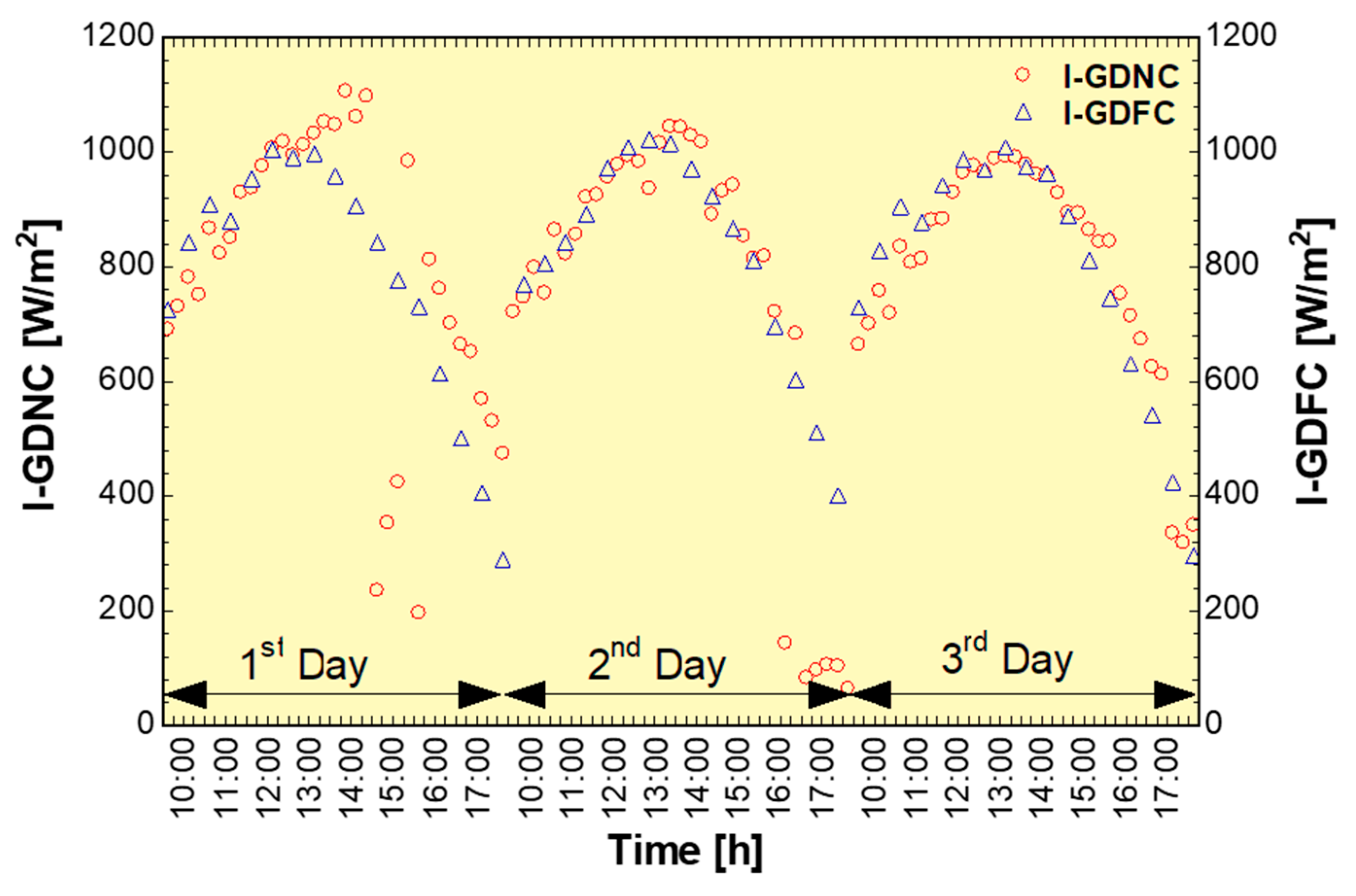
In this study, the product (grape) was dried using natural and forced convection processes in a solar greenhouse dryer. Convective heat transfer coefficient values, which have been paid great attention to in the literature, were calculated for the data obtained from the experiments and especially for designing of the drying systems. Parameters (such as climatic conditions in the greenhouse, product temperature, and the amount of moisture evaporated from the product) used to determine the h_c values are directly affected by radiation in the greenhouse type dryers. In Figure 4, changes in the radiation values of the days of drying in natural (GDNC) and forced (GDFC) convection were given during the drying process. During the drying period, it was observed that the irradiation values in the grape-drying process with GDNC were higher than the radiation values in the grape-drying process with GDFC.

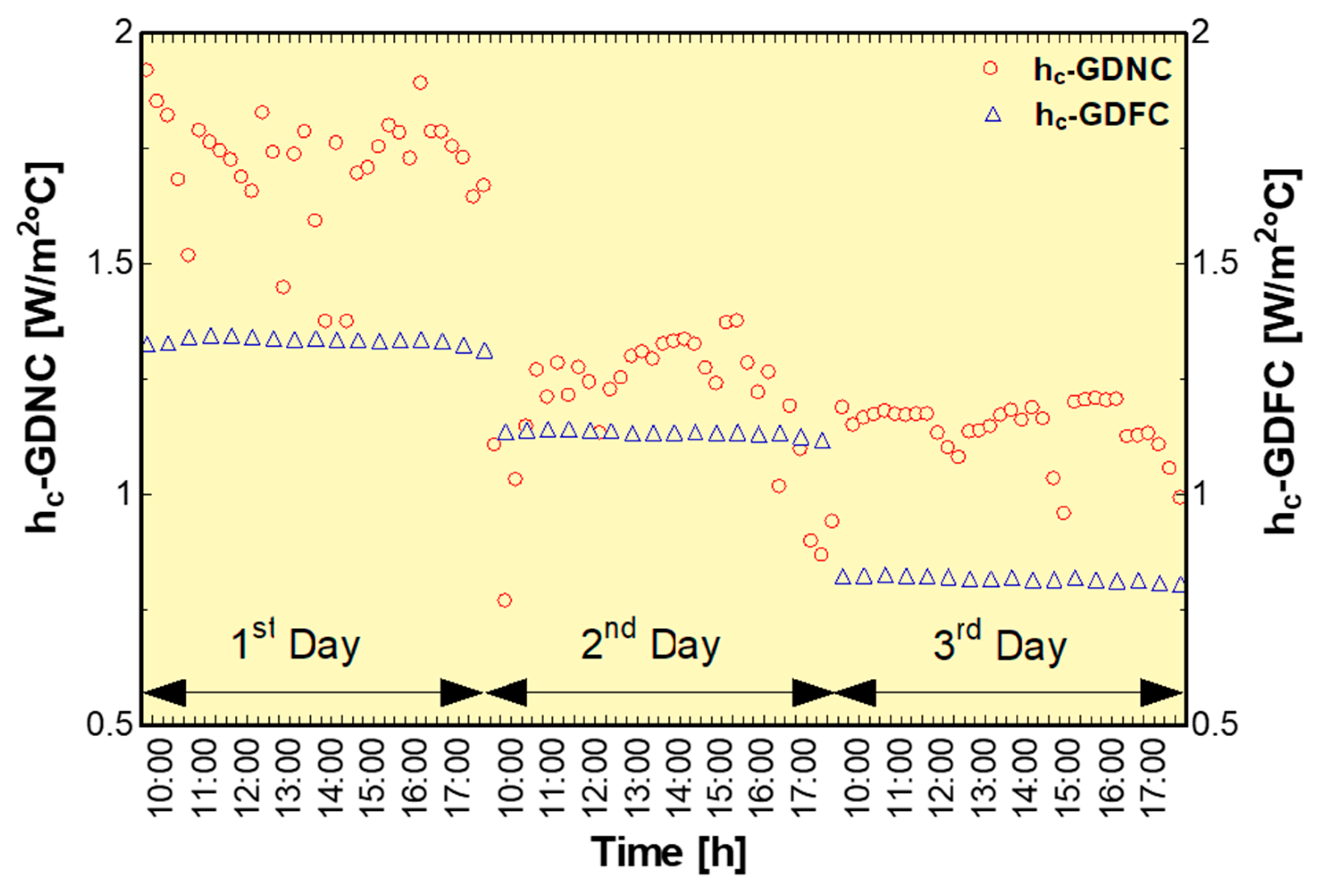
The convective heat transfer coefficient was determined by using the values obtained from the experimental data and the grape dried by different drying processes. Three-day convective heat transfer coefficients of GDNC- and GDFC-dried grape are given in Figure 5. When the graphs were analyzed, it was observed that convective heat transfer coefficient values obtained with GDNC are more volatile than the convective heat transfer coefficients obtained by GDFC. Both drying systems and grape drying showed a day-by-day decrease in h_c values. The highest convective heat transfer coefficient values were obtained with GDNC on the first day. In GDNC and GDFC, grape drying h_c values changed during the drying period: 0.77032–1.89053 W/m²°C and 0.80668–1.34593 W/m²°C, respectively. C and n values in grape drying with GDNC were obtained as 1.65168 and 0.070596, 0.66994 and 0.11680, and 1.10818 and 0.06444 for the first day, second day, and third day respectively. C and n values in grape drying with GDFC were obtained as 1.00479 and 0.11322, 1.00767 and 0.09376, and 0.99128 and 0.05773 for the first day, second day, and third day, respectively. The reasons for the higher h_c values of grapes dried by GDNC can be interpreted as the climatic conditions of the outdoor environment and the predominance of the thermophysical effects caused by natural circulation.

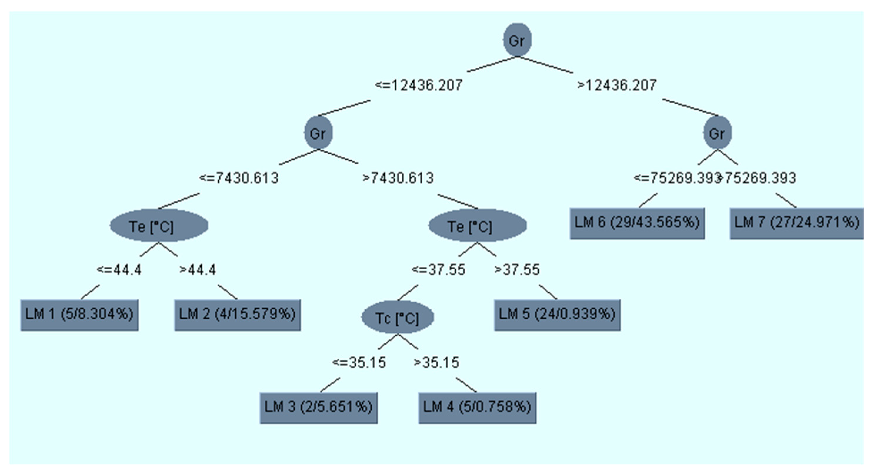
The decision tree structures for predicting the convective heat transfer coefficients obtained by drying grapes in GDNC and GDFC are given in Figure 6 and Figure 7, respectively.

Figure 6 shows the tree structure used by the decision tree algorithm to estimate h_c values. In Figure 6, the heat transfer coefficient was estimated according to the rules in the tree branches, depending on the values of Gr, T_e and T_c in the decision tree. In Figure 6, the Grashof number (Gr) parameter forms the root part of the tree, T_e and T_c form the inner root, and LM1-7 forms the leaves. The DT algorithm continues to apply rules until the data is separated by the decisions in the branches and reaches the LM values. DT algorithm sets the rules and roots randomly.

Figure 7 shows the tree structure used by the decision tree algorithm to estimate h_c values. In Figure 7, the heat transfer coefficient was estimated according to the rules in the branches of trees depending on the values of T_c, T_e, Ɣ and m_ev in the decision tree. In Figure 7, the T_c parameter forms the root part of the tree; Ɣ, T_e and m_ev form the inner root; and LM1-8 forms the leaves. The DT algorithm continues to apply rules until the data is separated by the decisions in the branches and reaches the LM values. The DT algorithm sets the rules and roots randomly. When both DT models were examined, it was seen that although similar input parameters (T_c, T_e, Ɣ and m_ev) are used, except for Re and Gr numbers, the DT tree structures were composed of different parameters.

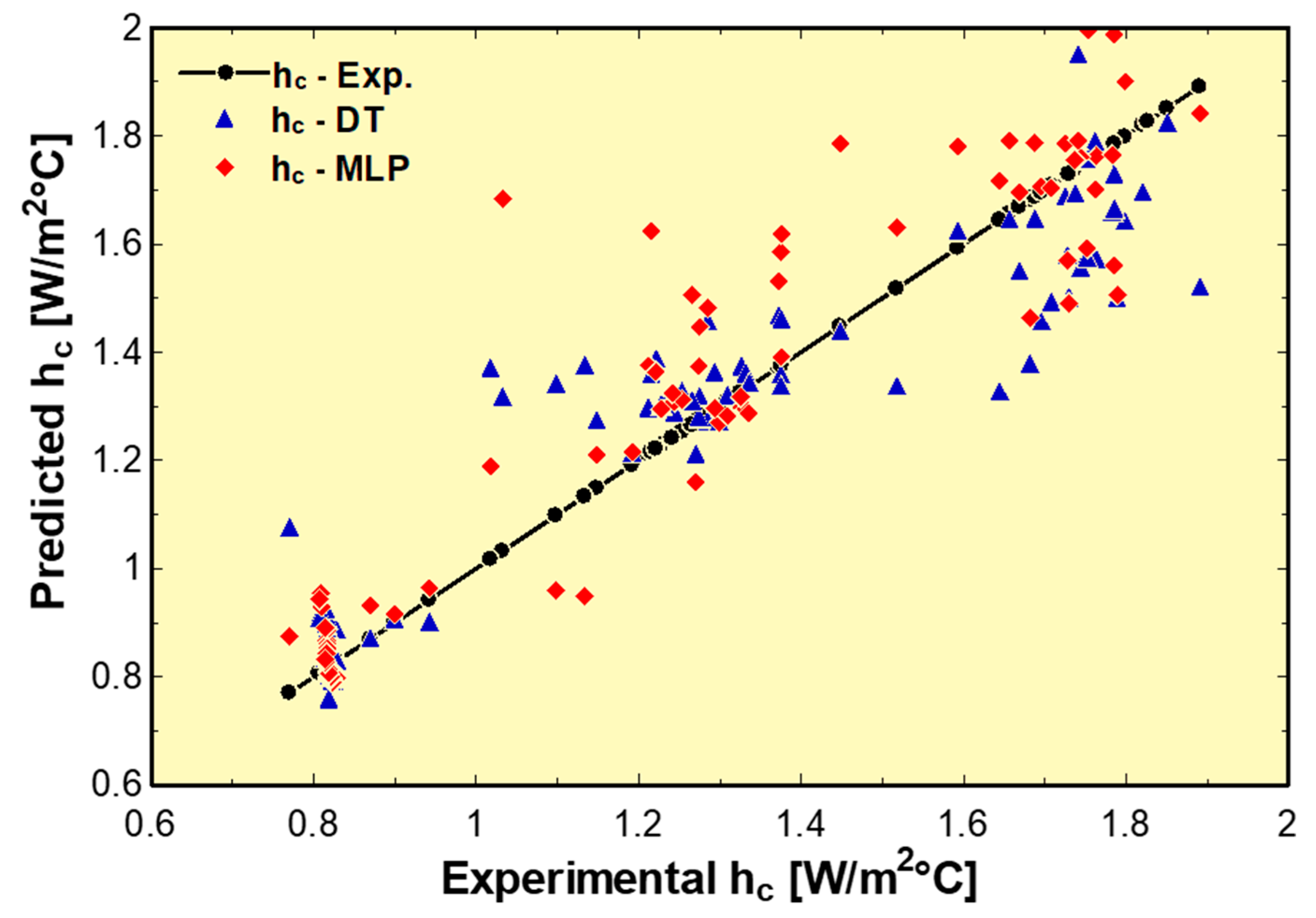
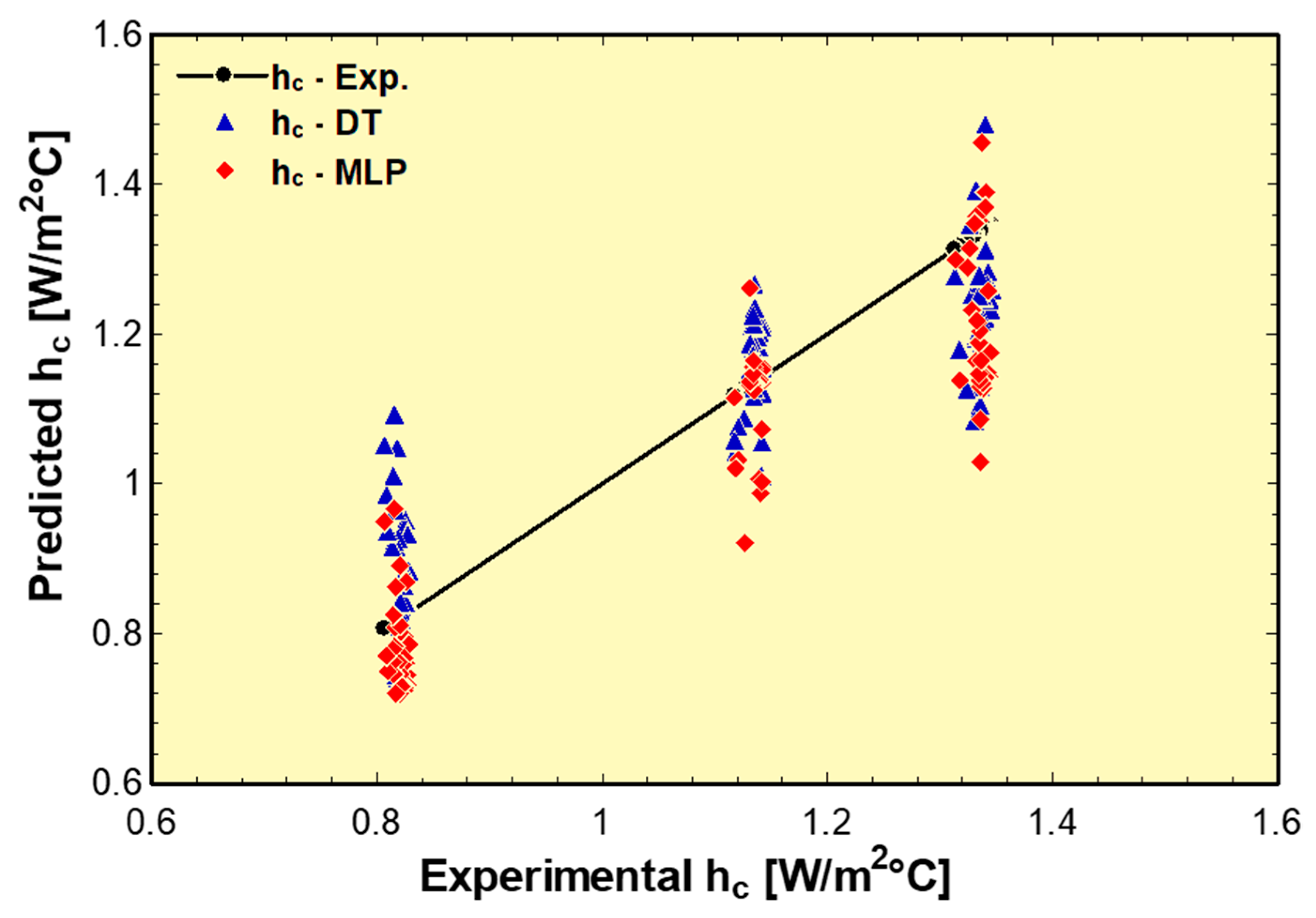
Different estimators were used with the calculated data, in an effort to secure results with faster and higher accuracy. MLP and DT methods were used as predictors. The variation of the convective heat transfer coefficient values obtained by three-day experimental (actual) and predictive methods by GDNC and GDFC is shown in Figure 8 and Figure 9, respectively.

In Figure 8 and Figure 9, the predictive h_c values obtained by the machine algorithms with the h_c values calculated by experimental data are close. The h_c values obtained by two different estimators, DT and MLP, were estimated. Statistical analysis parameters, root mean squared error (RMSE), and relative absolute error (RAE) values were calculated (

Table 5. Error rates for DT and MLP predicts.

Drying Method	Predictor	MAE	RMSE	RAE
GDNC	DT	0.0903	0.1286	0.27
	MLP	0.0990	0.1438	0.29
GDFC	DT	0.0909	0.1098	0.34
	MLP	0.0815	0.1088	0.32

).

Many researchers have obtained the heat transfer coefficient for different applications by means of different estimators. They have considered statistical error rates according to the convective heat transfer coefficients obtained experimentally for the accuracy of the estimators they use. When the results in the literature were examined, it was observed that the error analysis results obtained in the study are consistent (

Table 6. Heat transfer coefficient values and error analysis results obtained using different estimators for different applications in the literature.

Predicted Parameter	System	Total Data	Model	Result	Reference
Thermal Efficiency	Medium-temperature point-focus solar collector	72	ANN	RMSE = 0.4495	[51]
Solar Radiation	The meteorological data	288	MLP RBF	RMSEMLP = 0.351 RMSERBF = 0.401	[52]
Thermal Efficiency	Solar still	720	ANN	RMSE = 1.147	[54]
Heat flux	Pool boiling	1400	DT MLP	RMSEDT = 4.2 RMSEMLP = 4.6	[50]
Viscosity	CuO, pure water, ethanol and ethylene glycol-based nanofluids	1620	DT MLP	RMSEDT = 0.14 RMSEMLP = 0.07	[53]
Convective heat transfer coefficient	Air heated solar collector dryer	600	SVM	RMSE = 0.335	[31]

).

4. Conclusions

The convective heat transfer coefficient is an important parameter in terms of drying speed and drying kinetics, because the temperature difference in air and product varies with it. In this study, natural and forced convection solar greenhouse dryers were designed. Grape was the product to be dried and its convective heat transfer coefficients were calculated.

• The average heat transfer coefficient values of the grapes dried by GDNC and GDFC were obtained as 1.24 W/m²°C and 1.10 W/m²°C, respectively. The convective heat transfer coefficient value of the grape dried by forced convection decreased by 11.3% compared to the convective heat transfer coefficient of the grape dried by natural convection. The average values in the two drying processes were not largely different, the reasons for which could be the outer transparent cover material of the greenhouse, climatic conditions, thermophysical properties of the product, and porosity structure.
• Within the scope of this study, it was observed that a higher convective heat transfer coefficient value (h_c) was obtained with a ventilation chimney, which was formed for the realization of natural convection (GDNC) in the greenhouse without any energy consumption. On doing so, the product was protected from the harmful effects of an outdoor environment, and good heat transfer is achieved for the drying process.
• The predictive models for estimating convective heat transfer coefficient (h_c) were obtained by using computational intelligence algorithms, which is important in terms of the use of computational intelligence methods in solar greenhouse drying systems. MAE, RMSE, and RAE error analyses were performed to determine the accuracy of the obtained models. According to the results of the error analysis, the DT algorithm in GDNC was approximately 10% more accurate than MLP. In the GNFC, the MLP algorithm was approximately 10% more accurately than the DT.
• In addition, although the other input parameters were the same, except the Reynolds and Grashof numbers parameters, the decision tree structures were formed differently for both drying systems. It was observed that these parameters have different values and therefore their effect on convective heat transfer coefficient values are different, and the decision tree structures are different.
• The values of experimental and predictive convective heat transfer coefficients are very close. In different drying systems, different products can be dried, more data obtained, and more successful prediction models created by using different computational intelligence methods.
• It was observed that the coefficient can be used in the DT and MLP models to estimate h_c values, which are of great importance in designing drying cabinets.

References

- Amjad, W.; Munir, A.; Esper, A.; Hensel, O. Spatial homogeneity of drying in a batch type food dryer with diagonal air flow design. J. Food Eng. 2015, 144, 148–155. [Google Scholar] [CrossRef]
- Tiwari, G.N. Greenhouse Technology for Controlled Environment; Narosa Publishing House: New Delhi, India, 2003. [Google Scholar]
- Hossain, M.A.; Amer, B.M.A.; Gottschalk, K. Hybrid solar dryer for quality dried tomato. Dry. Technol. 2008, 26, 1591–1601. [Google Scholar] [CrossRef]
- Fernandez-García, A.; Rojas, E.; Perez, M.; Silva, R.; Hernandez-Escobedo, Q.; Manzano-Agugliaro, F. A parabolic-trough collector for cleaner industrial process heat. J. Clean. Prod. 2015, 89, 272–285. [Google Scholar] [CrossRef]
- Perea-Moreno, A.J.; Juaidi, A.; Manzano-Agugliaro, F. Solar greenhouse dryer system for wood chips improvement as biofuel. J. Clean. Prod. 2016, 135, 1233–1241. [Google Scholar] [CrossRef]
- Tong, X.; Sun, Z.; Sigrimis, N.; Li, T. Energy sustainability performance of a sliding cover solar greenhouse: Solar energy capture aspects. Biosyst. Eng. 2018, 102, 176. [Google Scholar] [CrossRef]
- Rovense, F. A Case of Study of a Concentrating Solar Power Plant with Unfired Joule-Brayton Cycle. Energy Procedia 2015, 82, 978–985. [Google Scholar] [CrossRef] [Green Version]
- Nastasi, B.; di Matteo, U. Solar energy technologies in Sustainable Energy Action Plans of Italian big cities. Energy Procedia 2016, 101, 1064–1071. [Google Scholar] [CrossRef]
- Prakash, O.; Kumar, A. A Solar greenhouse drying: A review. Renew. Sustain. Energy Rev. 2014, 29, 905–910. [Google Scholar] [CrossRef]
- Chauhan, P.S.; Kumar, A. Performance analysis of greenhouse dryer by using insulated north-wall under natural convection mode. Energy Rep. 2016, 2, 107–116. [Google Scholar] [CrossRef] [Green Version]
- Tiwari, G.N.; Barnwal, P. Fundamentals of solar dryers Anamaya; Anamaya Publishers: New Delhi, India, 2011. [Google Scholar]
- Prakash, O.; Kumar, A. Environomical analysis and mathematical modelling for tomato flakes drying in a modified greenhouse dryer under active mode. Int. J. Food Eng. 2014, 10, 669–681. [Google Scholar] [CrossRef]
- Prakash, O.; Kumar, A. Historical review and recent trends in solar drying systems. Int. J. Green Energy 2013, 10, 690–738. [Google Scholar] [CrossRef]
- Tiwari, G.N.; Kumar, A. Evaluation of convective mass transfer coefficient during drying of jaggery. J. Food Eng. 2004, 63, 219–227. [Google Scholar] [CrossRef]
- Leon, M.A.; Kumar, S.; Bhattacharya, S.C. A comprehensive procedure for performance evaluation of solar food dryers. Renew. Sustain. Energy Rev. 2002, 6, 367–393. [Google Scholar] [CrossRef]
- Condori, M.; Saravia, L. Analytical model for the performance of the tunnel-type greenhouse dryer. Renew. Energy 2003, 28, 467–485. [Google Scholar] [CrossRef]
- Singh, S.; Kumar, S. Testing method for thermal performance based rating of various solar dryer designs. Solar Energy 2012, 86, 87–98. [Google Scholar] [CrossRef]
- Sharma, A.; Chen, C.R.; Lan, N.V. Solar-energy drying systems: A review. Renew. Sustain. Energy Rev. 2009, 13, 1185–1210. [Google Scholar] [CrossRef]
- Fudholi, A.; Sopian, K.; Bakhtyar, B.; Gabbasa, M.; Othman, M.Y.; Ruslan, M.H. Review of solar drying systems with air based solar collectors in Malaysia. Renew. Sustain. Energy Rev. 2015, 51, 1191–1204. [Google Scholar] [CrossRef]
- Chauhan, P.S.; Kumar, A.; Tekasakul, P. Applications of software in solar drying systems: A review. Renew. Sustain. Energy Rev. 2015, 51, 1326–1337. [Google Scholar] [CrossRef]
- Kumar, A.; Tiwari, G.N.; Kumar, S.; Pandey, M. Role of greenhouse technology in agricultural engineering. Int. J. Agric. Res. 2006, 1, 364–372. [Google Scholar]
- Condori, M.; Saravia, L. The performance of forced convection greenhouse driers. Renew. Energy 1998, 13, 453–469. [Google Scholar] [CrossRef]
- Kumar, A.; Tiwari, G.N. Thermal modeling of a natural convection greenhosue drying system for jaggery: An experimental validation. Sol. Energy 2006, 80, 1135–1144. [Google Scholar] [CrossRef]
- Prakash, O.; Kumar, A. ANFIS modelling of a natural convection greenhouse drying system for jaggery: An experimental validation. Int. J. Sustain. Energy 2014, 33, 316–335. [Google Scholar] [CrossRef]
- Jain, D.; Jain, R.K. Performance evaluation of an inclined multi-pass solar air heater with inbuilt thermal storage on deep-bed drying application. J. Food Eng. 2004, 65, 497–509. [Google Scholar] [CrossRef]
- Bala, B.K.; Mondol, M.R.A.; Biswas, B.K.; Chowdury, B.L.D.; Janjai, S. Solar drying of pineapple using solar tunnel dryer. Renew. Energy 2003, 28, 83–190. [Google Scholar] [CrossRef]
- Dinçer, İ.; Zamfirescu, C. Drying Phenomena-Theory and Applications; John Wiley & Sons, Inc.: West Sussex, UK, 2016. [Google Scholar]
- Akpinar, E.K. Evaluation of convective heat transfer coefficient of various crops in cyclone type dryer. Energy Convers. Manag. 2005, 46, 2439–2454. [Google Scholar] [CrossRef]
- Akpinar, E.K. Experimental investigation of convective heat transfer coefficient of various agricultural products under open sun drying. Int. J. Green Energy 2005, 1, 429–440. [Google Scholar] [CrossRef]
- Goyal, R.K.; Tiwari, G.N. Heat and mass transfer relations for crop drying. Dry. Technol. 1998, 16, 1741–1754. [Google Scholar] [CrossRef]
- Das, M.; Akpinar, E.K. Investigation of Pear Drying Performance by Different Methods and Regression of Convective Heat Transfer Coefficient with Support Vector Machine. Appl. Sci. 2018, 8, 215. [Google Scholar] [CrossRef]
- Acikgoz, O.; Çebi, A.; Dalkilic, A.S.; Koca, A.; Çetin, G.; Gemici, Z.; Wongwises, S. A novel ANN-based approach to estimate heat transfer coefficients in radiant wall heating systems. Energy Build. 2017, 144, 401–415. [Google Scholar] [CrossRef]
- Hassanpour, M.; Vaferi, B.; Masoumi, M.E. Estimation of pool boiling heat transfer coefficient of alümina water-based nanofluids by various artificial intelligence (AI) approaches. Appl. Eng. 2018, 128, 1208–1222. [Google Scholar] [CrossRef]
- Verma, T.N.; Nashine, P.; Singh, D.V.; Singh, T.S.; Panwar, D. ANN Prediction of an experimental heat transfer analysis of concentric tube heat exchanger with corrugated inner tubes. Appl. Eng. 2017, 120, 219–227. [Google Scholar] [CrossRef]
- Romero-Méndez, R.; Lara-Vázquez, P.; Oviedo-Tolentino, F.; Martín, D.-G.H.; Gerardo, P.-G.F.; Arturo, P.V. Use of Artificial Neural Networks for Prediction of the Convective Heat Transfer Coefficient in Evaporative Mini-Tubes. Ing. Investig. Tecnol. 2016, 17, 23–34. [Google Scholar] [CrossRef] [Green Version]
- Rokach, L.; Maimon, O. Data Mining with Decision Trees: Theory and Applications, 2nd ed.; World Scientific Publishing Co. Pte Ltd.: Singapore, 2015. [Google Scholar]
- Alonso, D.P.; Peña-Tejedor, S.; Navarro, M.; Rad, C.; Arnaiz-González, Á.; Díez-Pastor, J.-F. Decision Trees for the prediction of environmental and agronomic effects of the use of Compost of Sewage Sludge (CSS). Sustain. Prod. Consum. 2017, 12, 119–133. [Google Scholar] [CrossRef]
- Kumar, A.; Tiwari, G.N. Effect of shape and size on convective mass transfer coefficient during greenhouse drying (GHD) of jaggery. J. Food Technol. 2006, 73, 121–134. [Google Scholar] [CrossRef]
- Doymaz, İ. Sun drying of seedless and seeded grapes. J. Food Sci. Technol. 2012, 49, 214–220. [Google Scholar] [CrossRef] [PubMed]
- Kline, S.J.; McClintock, F.A. Describing Uncertainties in Single-Sample Experiments. Mech. Eng. 1953, 75, 3–8. [Google Scholar]
- Holman, J.P. Experimental Methods for Engineers, 5th ed.; Mc-Graw Hill Company: New York, NY, USA, 1989. [Google Scholar]
- Anwar, S.I.; Tiwari, G.N. Evaluation of convective heat transfer coefficient in crop drying under open sun drying conditions. Energy Convers. Manag. 2001, 42, 627–637. [Google Scholar] [CrossRef]
- Anwar, S.I.; Tiwari, G.N. Convective heat transfer coefficient of crop in forced convection drying—An experimental study. Energy Convers. Manag. 2001, 42, 1687–1698. [Google Scholar] [CrossRef]
- Aha, D.W.; Kibler, D.; Albert, M.K. Instance-based learning algorithms. Mach. Learn. 1991, 6, 37–66. [Google Scholar] [CrossRef] [Green Version]
- Guo, W.; Yang, Y.; Zhou, Y.; Tan, Y.; Wei, H.; Song, A.; Pang, G. Influence Area of Overlap Singularity in Multilayer Perceptrons. IEEE Access 2018, 6, 60214–60223. [Google Scholar] [CrossRef]
- Zhai, X.; Ali, A.A.S.; Amira, A.; Bensaali, F. MLP neural network based gas classification system on Zynq SoC. IEEE Access 2016, 4, 8138–8146. [Google Scholar] [CrossRef]
- Eslamian, S.S.; Gohari, S.A.; Zareian, M.J.; Firoozfar, A. Estimating Penman–Monteith reference evapotranspiration using artificial neural networks and genetic algorithm: A case study. Arab. J. Sci. Eng. 2012, 37, 935–944. [Google Scholar] [CrossRef]
- Li, Y.; Tang, G.; Du, J.; Zhou, N.; Zhao, Y.; Wu, T. Multilayer Perceptron Method to Estimate Real-World Fuel Consumption Rate of Light Duty Vehicles. IEEE Access 2019, 7, 63395–63402. [Google Scholar] [CrossRef]
- Safavian, S.R.; Landgrebe, D. A survey of decision tree classifier methodology. IEEE Trans. Syst. Man Cybern. 1991, 21, 660–674. [Google Scholar] [CrossRef]
- Alic, E.; Das, M.; Kaska, O. Heat Flux Estimation at Pool Boiling Processes with Computational Intelligence Methods. Processes 2019, 7, 293. [Google Scholar] [CrossRef]
- Gorjian, S.; Hashjin, T.T.; Ghobadian, B.; Banakar, A.A. Thermal performance evaluation of a medium-temperature point-focus solar collector using local weather data and artificial neural networks. Int. J. Green Energy 2015, 12, 493–505. [Google Scholar] [CrossRef]
- Al-Shamisi, M.H.; Assi, A.H.; Hejase, H.A. Artificial neural networks for predicting global solar radiation in Al Ain city-UAE. Int. J. Green Energy 2013, 10, 443–456. [Google Scholar] [CrossRef]
- Demirpolat, A.B. Investigation of Mass Transfer with Different Models in a Solar Energy Food-Drying System. Energies 2019, 12, 3447. [Google Scholar] [CrossRef]
- Mashaly, A.F.; Alazba, A.A. Comparison of ANN, MVR, and SWR models for computing thermal efficiency of a solar still. Int. J. Green Energy 2016, 13, 1016–1025. [Google Scholar] [CrossRef]
- Demirpolat, A.B.; Das, M. Prediction of Viscosity Values of Nanofluids at Different pH Values by Alternating Decision Tree and Multilayer Perceptron Methods. Appl. Sci. 2019, 9, 1288. [Google Scholar] [CrossRef]
Figure 1.
The experimental setup: (1—Drying Room, 2—Chimney, 3—Fan, 4—Reosta, 5—Digital Thermometer and Channel Selector, 6—Thermocouples, 7—Trays, 8—Scales, 9—Moisture Meter, 10—Solar Radiation Meter).
Figure 2.
Schematic representation of the drying process.
Figure 3.
MLP network structure.
Figure 4.
The change of I values according to time in GDNC and GDFC.
Figure 5.
The change of hc values according to time in GDNC and GDFC.
Figure 6.
Decision tree structure used to predict convective heat transfer coefficients of GDNC-dried grapes.
Figure 7.
Decision tree structure used to predict convective heat transfer coefficients of GDFC-dried grapes.
Figure 8.
Changes of experimental and predicted hc values of grapes dried in GDNC, according to the time taken.
Figure 9.
Changes of experimental and predicted hc values of grapes dried in GDFC, according to the time taken.