Long-Term Distributional Impacts of European Cap-and-Trade Climate Policies: A CGE Multi-Regional Analysis

Abstract

Carbon pricing is a policy with the potential to reduce CO₂ emissions in the household sector and support the European Union in achieving its environmental targets by 2050. However, the policy faces acceptance problems from the majority of the public. In the framework of the project Role of technologies in an energy efficient economy–model-based analysis of policy measures and transformation pathways to a sustainable energy system (REEEM), financed by the European Commission under the Horizon 2020 program, we investigate the effects of such a policy in order to understand its challenges and opportunities. To that end, we use a recursive-dynamic multi-regional Computable General Equilibrium model to represent carbon pricing as a cap-and-trade system and calculate its impacts on consumption of energy goods, incidence of carbon prices, and gross income growth for different income groups. We compare one reference scenario and four scenario variations with distinct CO₂ reduction targets inside and outside of the EU. The results demonstrate that higher emission reductions, compared to the reference scenario, lead to slower Gross Domestic Product growth, but also produce a more equitable increase of gross income and can help reduce income inequalities. In this case, considering that the revenues of carbon pricing are paid back to the households, the gross income of the poorest quintile grows as much as, or even more in some cases, than the gross income of the richest quintile.

1. Introduction

According to the Intergovernmental Panel for Climate Change (IPCC), anthropogenic emission of greenhouse gases has contributed to a global temperature increase, rising sea levels, and more frequent occurrences of extreme weather events [1]. The Paris Agreement puts forward a global plan to limit the growth in global temperature below 2 °C and to pursue the efforts to limit it to 1.5 °C to prevent further negative consequences of climate change [2].

Recent work on the economic consequences of climate change provides quantification on the possible costs if climate change is not controlled. Using detailed data on a global scale where the unit of observation was 1° latitude by 1° longitude cells, Nordhaus [3] finds a negative relationship between economic output and mean surface temperature. Using the estimated parameters and assuming an increase in the average temperature of 3 °C and a decrease in precipitation, he forecasts a reduction of economic activity between 0.9% and 3%. Based on the panel data of 100 most populous countries, Horowitz [4] estimates that a rise in the surface temperature of 1 °C would reduce the world GDP between 2.7% and 4.2%, with the best estimate being 3.8%. Hsiang [5] investigates the impact of variation of surface temperatures on the output of 28 Caribbean basin countries. After controlling for the effect of cyclones, he finds that a 1 °C rise in surface temperature is associated with a simultaneous decrease in GDP of 2.5%. He also finds that higher surface temperature is associated with a statistically significant decrease in economic output in three out of seven economic sectors. Dell et al. [6] find large and negative effects of higher temperatures on economic growth: they estimate that a 1 °C rise in temperature in a given year reduces economic growth in that year by about 1.3%, though the relationship is more ambiguous for rich countries. The possibility that climate change does not harm rich countries has prompted some researchers to investigate this issue further. Burke et al. [7] address this topic through the analysis of historical data to determine whether country-specific deviations from growth trends are related non-linearly to country-specific deviations from temperature and precipitation trends, after accounting for any disparities common to all countries. They find country-level economic production is smooth, non-linear, and concave in temperature, with a maximum at 13 °C. Both rich and poor countries exhibit similar non-linear responses to temperature. Therefore, the link between rich countries and temperature change is weaker primarily because rich countries exhibit lower temperatures. Lemoine and Kapnick [8] also find that future warming could raise the expected rate of economic growth in rich countries, reduce the expected rate of economic growth in poor countries, and increase the fluctuation of growth by increasing the climate’s variability.

To limit the growth of surface temperature caused by anthropogenic emissions of CO₂, policymakers often put either a carbon tax or an emissions trading scheme in place. The application of such mechanisms has proven to have negative economic consequences. Adams [9], by using a Computable General Equilibrium (CGE) model coupled with an electricity generation model, identified that the introduction of an Emissions Trading System (ETS) scheme in Australia would result in a real GDP decrease of 1.3% and a consumption loss of 1.4% by 2030. Real wages would decline by 3.3% and CO₂ emissions would be reduced by 21% compared to the baseline scenario. In a similar study, Adams et al. [10] analyzed the impact of carbon pricing on the Australian economy as part of a global ETS scheme, which resulted in 25% lower emissions in 2030, resulting in a reduction of GDP by 1.1% compared to a base case scenario, together with a reduction in household disposable income by 2.3% and real private consumption by 1.3%. They also show that despite affecting most industries, a carbon pricing policy has positive effects on some sectors, notably forestry, electricity generation from renewables, and electricity generation from gas (due to a move away from coal) as well as iron, steel, and aluminum, which become more internationally competitive due to cheaper raw material. Lu et al. [11] assess the impact of the introduction of a carbon tax on the Chinese economy and find that a carbon tax of up to 300 Chinese Yuan per ton of CO₂ (approximately 30 EUR in 2019) results in a relatively modest reduction of GDP of 1.1% compared to a scenario without a carbon tax. Similarly, Guo et al. [12] investigate the impact of the introduction of a carbon tax and also find negative effects on most of the economic sectors as well as the overall GDP and returns to labor and capital. In the European context, Panagiotis et al. [13] utilized an energy-system model with a CGE model to demonstrate that the Intended Nationally Determined Contribution (INDC) submitted by the European Union (EU-28) can be met with a minor GDP impact of 0.4% in 2030 and 1% in 2050 compared to the reference scenario.

Given research has shown that schemes to limit the emission of CO₂ into the atmosphere such as a carbon tax or an emission trading scheme entail a reduction in GDP growth and consumption, the issue of distributional impacts of such schemes arises. For example, poorer households tend to live in less energy-efficient homes, own energy-inefficient vehicles and appliances, and have lower incomes. Therefore, the increase in prices of energy-related goods hurts poor households disproportionately more than rich ones. In addition, due to the rise in prices of energy-related goods, poor households have to reduce their consumption of other goods. To make carbon tax-related policies acceptable and equitable, it is important to consider how they affect different members of society and to ensure that these policies are not regressive.

Related research includes Goulder [14], who emphasizes the importance of revenue recycling and tax interaction effects, both of which represent a fiscal interaction effect when assessing the cost-effectiveness of climate change policies. Revenue recycling refers to returning the revenues collected through climate change measures back to the economy, whilst tax interactions refer to the impact of climate policies on returns on factors of production. While the principles of revenue recycling effects are self-explanatory, the tax interactions argument states that climate policy measures increase the cost of carbon-related goods, hence driving up prices. This reduces the real wages of workers as well as returns to the owners of capital employing carbon-related inputs, both of which represent an efficiency loss. The efficiency loss could be reduced or even mitigated by applying appropriate fiscal policies such as the reduction of marginal tax rates on labor and capital, providing lump-sum transfers to households, or some combination of the above, depending upon the goals of the policymakers. Caron et al. [15] provide a five-model assessment of distributional impacts of carbon pricing in the U.S. To alleviate distributional impacts on different households they evaluate the efficiency and equity (progressivity) of lump-sum household transfers, capital, and labor tax reductions. They find that lump-sum transfers to the household consumer are progressive, but come at the greatest costs, while capital tax reductions are mostly regressive and help the richest households. Labor tax credits are somewhere in between these two measures. Nevertheless, the authors conclude that by using a creative approach such as lump-sum transfers to the poorest households and capital tax reductions, the policymakers can reduce the progressivity of carbon pricing at a rather low cost. Reaños and Lynch [16] evaluate the impact of a carbon tax in Ireland on sectors not covered by the ETS system. They also find that a carbon tax is regressive, hurting poor households the most. To alleviate the tax burden on households, they evaluate the impact of a flat rate and a targeted revenue recycling mechanism. Here they find poor households are better off receiving targeted support as opposed to a lump-sum payment, i.e., targeted measures are better suited to eliminate income inequality arising from the introduction of a carbon tax. In terms of administrative costs, they posit that a targeted approach would be more efficient as it would be conducted through the existing welfare system channels, while a lump-sum transfer to all households would require the establishment of a new channel to disburse the funds. Work by Tran et al. [17] analyzed the impact of emission reduction in Australia by 2020 by using a static CGE model. Without revenue compensating mechanisms, they find a decline in Australia’s GDP by 0.285%–0.3% by 2020 as well as a decrease in welfare for all 20 household categories. To address the issue of welfare loss in different households, they assess the use of direct lump sum transfers, government transfers, and reductions in income tax. They find a trade-off between efficiency and equity. While income tax policies are the most efficient in the sense that they achieve the highest reductions in the GDP losses, they are the least equitable as they mostly benefit the wealthiest households. On the other hand, lump sum transfers aid the poorest households, while government transfer policy mostly aids middle-income households.

Finally, there is a group of studies focused on a tax reform that shifts the burden of taxation from conventional taxes, such as on labor or value-added tax (VAT), to environmentally damaging activities. Such reform is also known as environmental tax reform (ETR) or green tax (or budget) reform (GTR). Maxim and Zander [18] analyzed the effects of substituting existing taxes by environmental taxes in European and non-European countries and found that an ETR has an average positive impact in employment for the European countries of 0.67% compared to the reference, but this number is highly dependent of the tax being substituted and varies from −0.15% for personal income tax (PIT) to 1.62% for VAT. Freire-González and Ho [19] use a CGE model to assess the effects of an ETR in Spain for three different levels of carbon taxes and four revenue recycling scenarios and discover a positive economic output in all scenarios for a tax level of €10/tCO₂ and some scenarios for a tax level of €20/tCO₂. Streimikiene et al. [20] researched on the impacts of environmental taxes in the Baltic region (Lithuania, Latvia, and Estonia) between 2005 and 2015 and revealed that an increase in the proportion of environmental taxes had a significant positive impact on sustainable energy development in that region.

In summary, the research up to date provides us with the following conclusions:

• The historic effects of climate change on economic growth have been documented, and they affect not only the magnitude but also the rate of economic growth.
• Unmitigated climate change results in significant negative environmental consequences that have negative repercussions on economic growth.
• To mitigate the economic consequences of climate change, policymakers should enact policies that will eliminate and hopefully reverse the effects of climate change. But these policies come at a cost and are regressive in nature, mostly hurting poor households.
• Policymakers have different options of revenue recycling mechanisms which fall in a range between efficient but inequitable (mitigation of negative effects of climate policies on economic output at the lowest costs but hurting poor households) and equitable but inefficient (a measure that supports more poor households than rich but comes at a higher cost).

Our paper adds to the current debate in several aspects. To our knowledge, this is the first comprehensive paper that addresses the consequences of the Paris Agreement on European economies, taking into account different pathways and their impacts on social disparities. In this sense, it expands the existing literature by making a multi-regional analysis of selected European countries between the years 2011 and 2050 while considering different emission targets inside and outside of the EU-28. Additionally, this work gives special attention to the distributional impacts from energy policies on different income groups by analyzing the income development, consumer behavior, and incidence of carbon prices for each income group.

A global multi-region recursive-dynamic CGE model with the household sector disaggregated into five income quintiles, similar to the approach from Bouet et al. [21], was applied for this work. Additionally, we employed one reference scenario and four scenario variations with different degrees of CO₂ emissions cuts. The results indicate that higher emission reductions, compared to the reference scenario, lead to slower GDP growth, but also induce a more equitable increase of gross income. In this case, the gross income of the poorest quintile grows as much as, or even more in some cases, than the gross income of the richest quintile, given that the revenues from pricing carbon are paid back to the households.

2. Materials and Methods

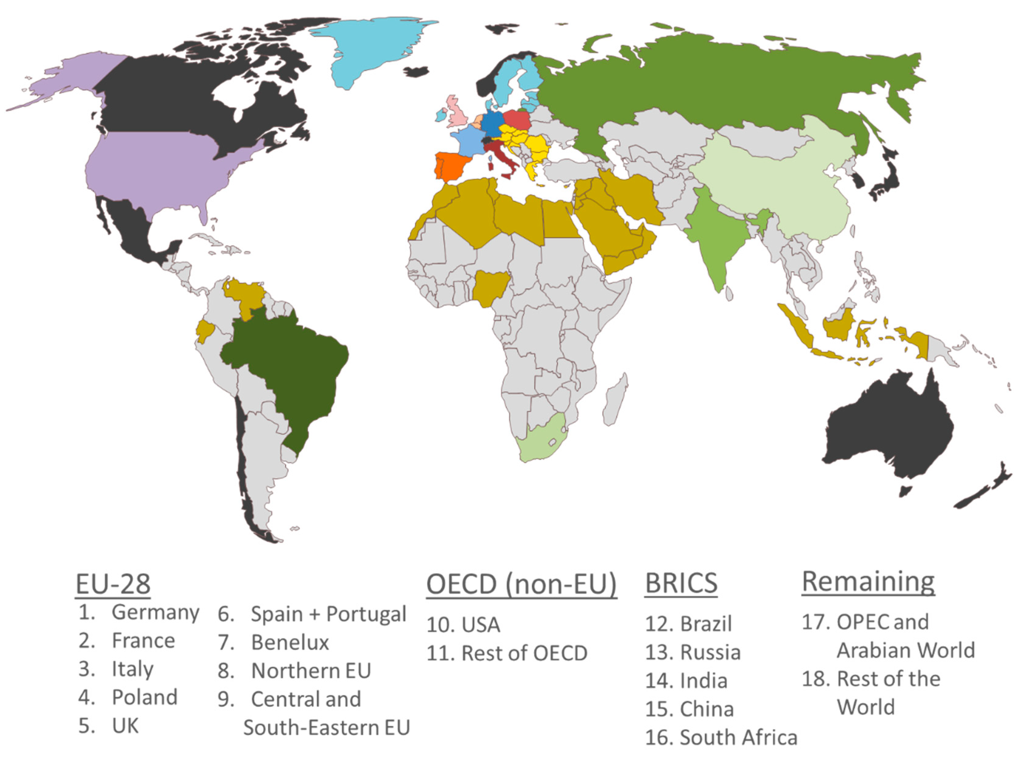
In this work, we use the CGE model NEWAGE (National European World Applied General Equilibrium, for more details about the NEWAGE model, visit https://www.ier.uni-stuttgart.de/forschung/modelle/NEWAGE/index_en.html) to analyze different scenarios. NEWAGE is a multi-region, multi-sector, recursive-dynamic general equilibrium model that depicts the production and distribution of commodities in the global economy. A total of 18 regions of the world are modeled, as shown in Figure A3, from which 9 regions are within EU-28, as shown in

Table 1. National European World Applied General Equilibrium (NEWAGE) Regions in the European Union.

NEWAGE Region	Countries
Germany	Germany
France	France
Italy	Italy
Poland	Poland
United Kingdom	United Kingdom
Spain + Portugal	Portugal, Spain
Benelux	Belgium, Luxembourg, Netherlands
Northern EU	Denmark, Estonia, Finland, Ireland, Latvia, Lithuania, Sweden
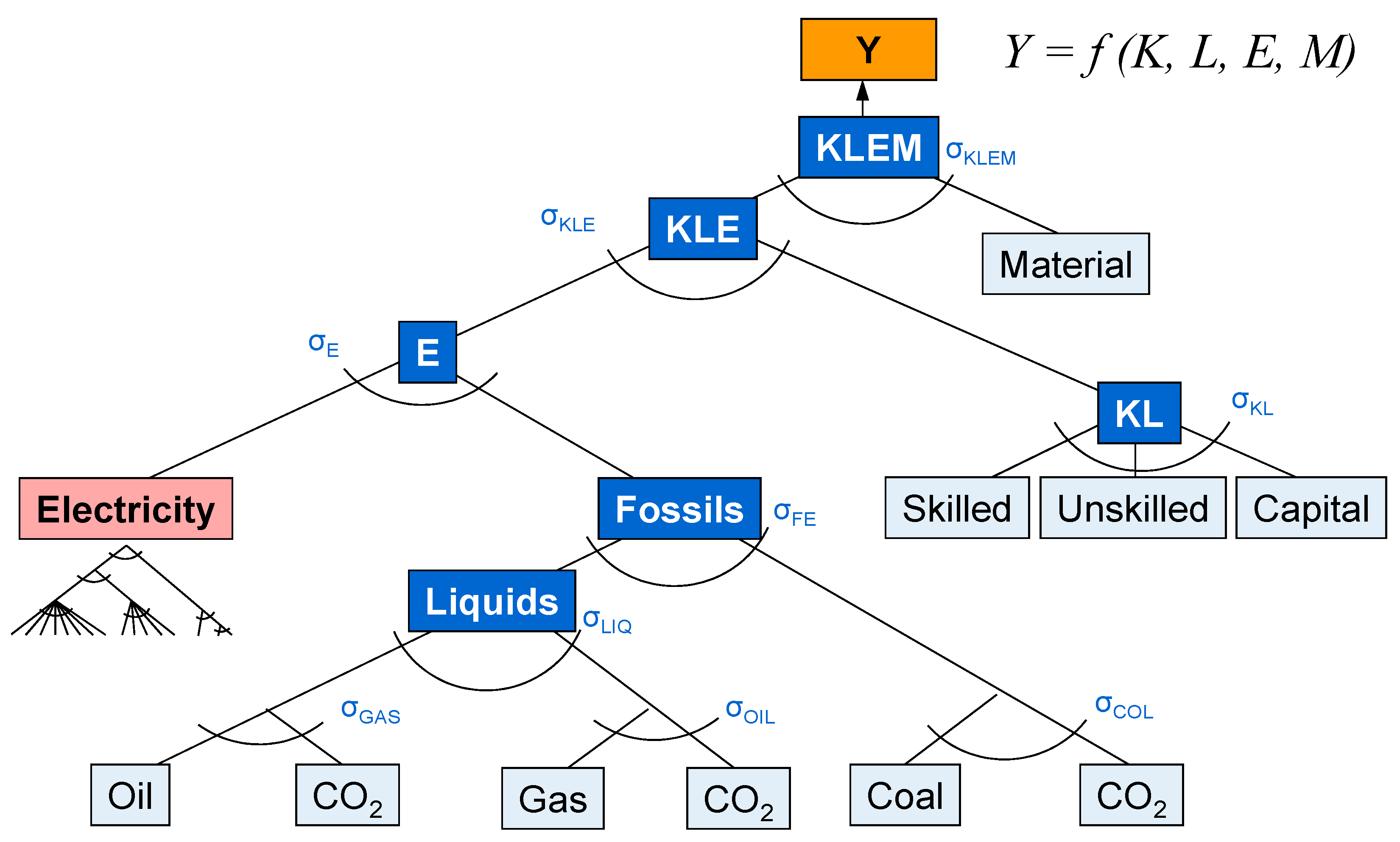
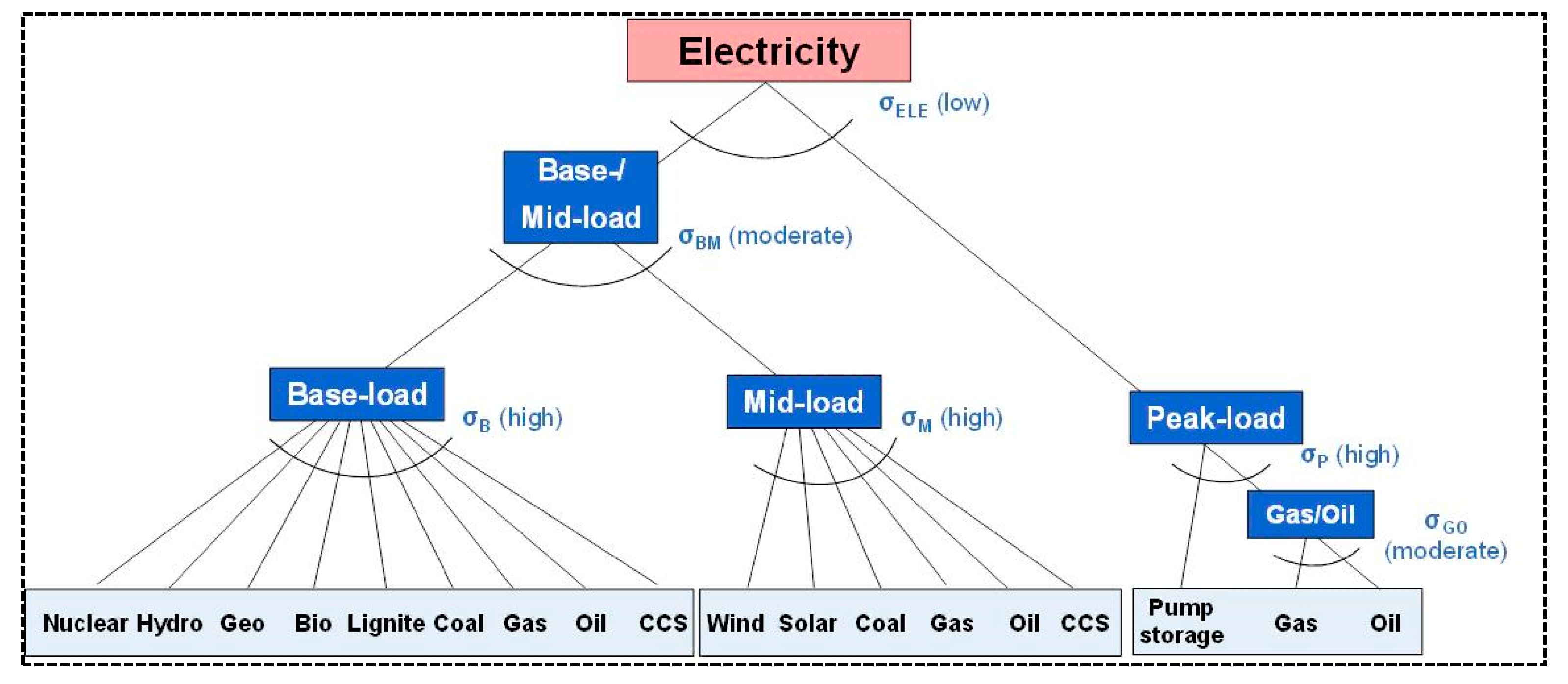
Central and South-Eastern EU	Austria, Bulgaria, Croatia, Cyprus, Czech Rep., Greece, Hungary, Malta, Romania, Slovakia, Slovenia

. The production sector is disaggregated into 5 energy production sectors, 6 energy-intensive industry sectors, 3 sectors representing the rest of the industry, and 4 sectors representing the rest of the economy. Additionally, it has a detailed representation of the electricity sector, consisting of 18 electricity generation technologies. Production possibilities are represented by Cobb-Douglas, Leontief, and Constant Elasticity of Substitution (CES) production functions. Detailed information regarding NEWAGE’s regional and sectoral structure, as well as the CES nesting for sectorial and electricity production, can be found in Appendix A of this paper.

The framework of NEWAGE enables the analysis of the impacts of different political interventions on macro-economic indicators, such as GDP growth, employment, or competitiveness. In contrast, energy system models are usually unable to assess overall macro-economic costs because they usually lack the relationship with other actors of the economy, despite having a richer depiction of the technologies within the energy sector. Therefore, NEWAGE is a valuable tool for the analysis of energy policies and its implications to the rest of the economy, especially regarding effects on the households sector.

Despite being able to represent the relationship among different sectors of the economy, NEWAGE cannot endogenously calculate technology development. The model is capable of substituting energy purchases by capital in the current time-step using CES nesting, however, it is not capable of investing in technology development to improve the energy efficiency of specific production sectors and reduce its sectoral energy consumption in the next time-step. To overcome this limitation, NEWAGE applies exogenous assumptions for the technology development from 2011 to 2050 through the Autonomous Energy Efficiency Index (AEEI) parameter, which was developed based on the energy efficiency improvements provided by the EU Reference Scenario [22]. For this work, the same set of AEEI was applied in all pathways, meaning that regardless of the environmental ambition, the rate of technology development remains the same. Additionally, the figures of electricity generation in the EU-28 between 2011 and 2050 utilized in this work were obtained through an iterative process that coupled the NEWAGE model with the energy system model TIMES-PanEU, as explained in [23].

The present version of NEWAGE model perceives the gains and losses of any policy measure solely as a matter of profit and costs. It means that the model is not capable of accounting the non-financial impacts brought by different pathways, such as increased air quality and lower water pollution, in the cases where emission levels decrease, or higher temperatures, in the case where countries fail to reduce emissions.

A central assumption influencing the choice of production factors and technologies are the Elasticities of Substitution (EoS) of the production functions. They define how easily production factors, e.g., capital and labor, or different technologies, e.g., photovoltaics and wind turbines, can substitute for each other. Figure A1 and Figure A2 show a graphical representation of NEWAGE’s production functions. Substitution parameters vary between zero and infinity, with a value equal to zero meaning substitution is not possible. The higher the elasticity value, the easier it is to substitute the two respective factors. The elasticity parameters in NEWAGE, primarily based on reference [24] and reference [25], are summarized in

Table A3. Substitution elasticities in NEWAGE for consumption.

CES Parameter	Substitution Elasticity Between	Value
σC-ENE	energy and non-energy-goods aggregate	0.5
σC-NE	non-energy-goods	1
σC-E	energy carriers (electricity, gas, oil, coal)	1
σC-GAS	gas and CO2 emissions	0
σC-OIL	oil and CO2 emissions	0
σC-COL	coal and CO2 emissions	0

,

Table A4. Substitution elasticities in NEWAGE for industry production.

CES Parameter	Substitution Elasticity Between	Value
σKLEM	material and capital-labor-energy	0
σKLE	Capital, labor and energy	0.5
σKL	capital, skilled and unskilled labor	1
σKL-refOil	capital, skilled and unskilled labor	0.2
σLAB	skilled and unskilled labor	0.5
σE	electricity and fossil fuels	0.1
σFE	Liquid and solid fossil fuels	0.5
σLQD	gas aggregate and oil aggregate	2
σOIL	oil and CO2 emissions	0
σCOL	coal and CO2 emissions	0
σGAS	gas and CO2 emissions	0

,

Table A5. Substitution elasticities in NEWAGE for electricity production.

CES Parameter	Substitution Elasticity Between	Value
σELE	base-, mid- and peak-load	0.8
σPL	electricity generation technologies peak-load	5
σOG	Peak-load gas and oil turbines	2.5
σBM-EU	base- and mid-load for EU-28 regions	5
σBM-RoW	base- and mid-load for non-EU-28 regions	4
σBL	electricity generation technologies base-load	8
σML	electricity generation technologies mid-load	5

, and

Table A6. Substitution elasticities in NEWAGE for trade.

CES Parameter	Substitution Elasticity Between	Value
σA	Armington Elasticity (substitution between local production and imported goods)	4
σIM	imported goods from different countries	8
σTS	imported good and associated transport service	0

.

In addition to the assumptions above, we use the following data sources for additional input parameters:

• GTAP 9 Data Base [26] for trade and energy data for the year 2011;
• Electricity Information 2013 [27] for electricity generation per country for the year 2011;
• EU Reference Scenario 2016 [22] for GDP growth for the EU-28 regions between years 2011 and 2050 and CO₂ emission for the EU-28 regions between years 2011 and 2050;
• The Great Shift: Macroeconomic projections for the world economy at the 2050 horizon [28] for GDP growth for the non-EU-28 regions between years 2011 and 2050 and CO₂ emissions for the non-EU-28 regions between years 2011 and 2050;
• Household budget survey (HBS) [29] for disaggregation of expenses;
• Survey on income and living conditions (SILC) [30] for income disaggregation.

In the context of CGE models, the representative agent is in many cases a combined depiction of government and households. It collects regional taxes, has a combined consumption of the two economic actors and represents and possesses endowments of three production factors: capital, labor and natural resources. Additionally, NEWAGE differentiates labor into two categories: skilled and unskilled, natural resources are divided into three categories: oil, natural gas, and coal, and adds CO₂ allowances as a fourth production factor for the implementation of cap-and-trade policies.

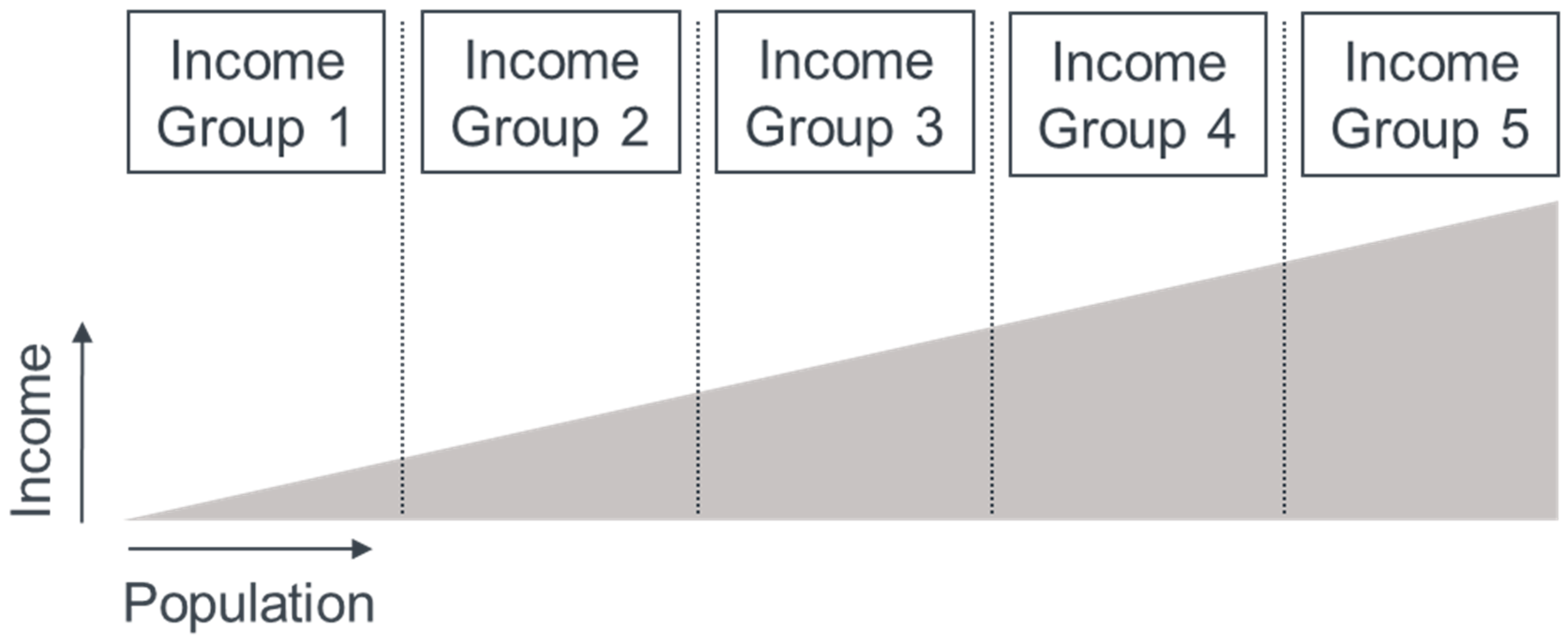
For the task of analyzing distributional effects on households, we amended the present representation of the representative agent in NEWAGE by disaggregation into six new blocks: one for the government and five for each of the income quintiles. More specifically, we divided the households into five equally sized groups, containing 20% of the population each, according to their income sorted from lowest (hh1) to highest income (hh5), as shown in Figure 1. No distinction between urban and rural populations was made and the calculus for income included gains from labor, capital, and government subsidies.

In order to perform the disaggregation of the household sector into five income groups, the first step was to separate the consumption of the representative agent between government and households, creating one block for each of these two agents. This task was executed by accessing the GTAP 9 database [26] to apply the consumption values for both agents and, later, implementing the two blocks replacing the original representative agent. Afterwards, as the data available for consumption and income sources was aggregated on a national level, it was necessary to use Eurostat’s Household Budgets Survey (HBS) [29] and Survey on Income and Living Conditions (SILC) [30] to disaggregate it into income groups. The two later databases were granted to the Lithuanian Energy Institute by Eurostat to be used in the REEEM Project (For more information, see reeem.org), to obtain data regarding the expenditure of households and their sources of income.

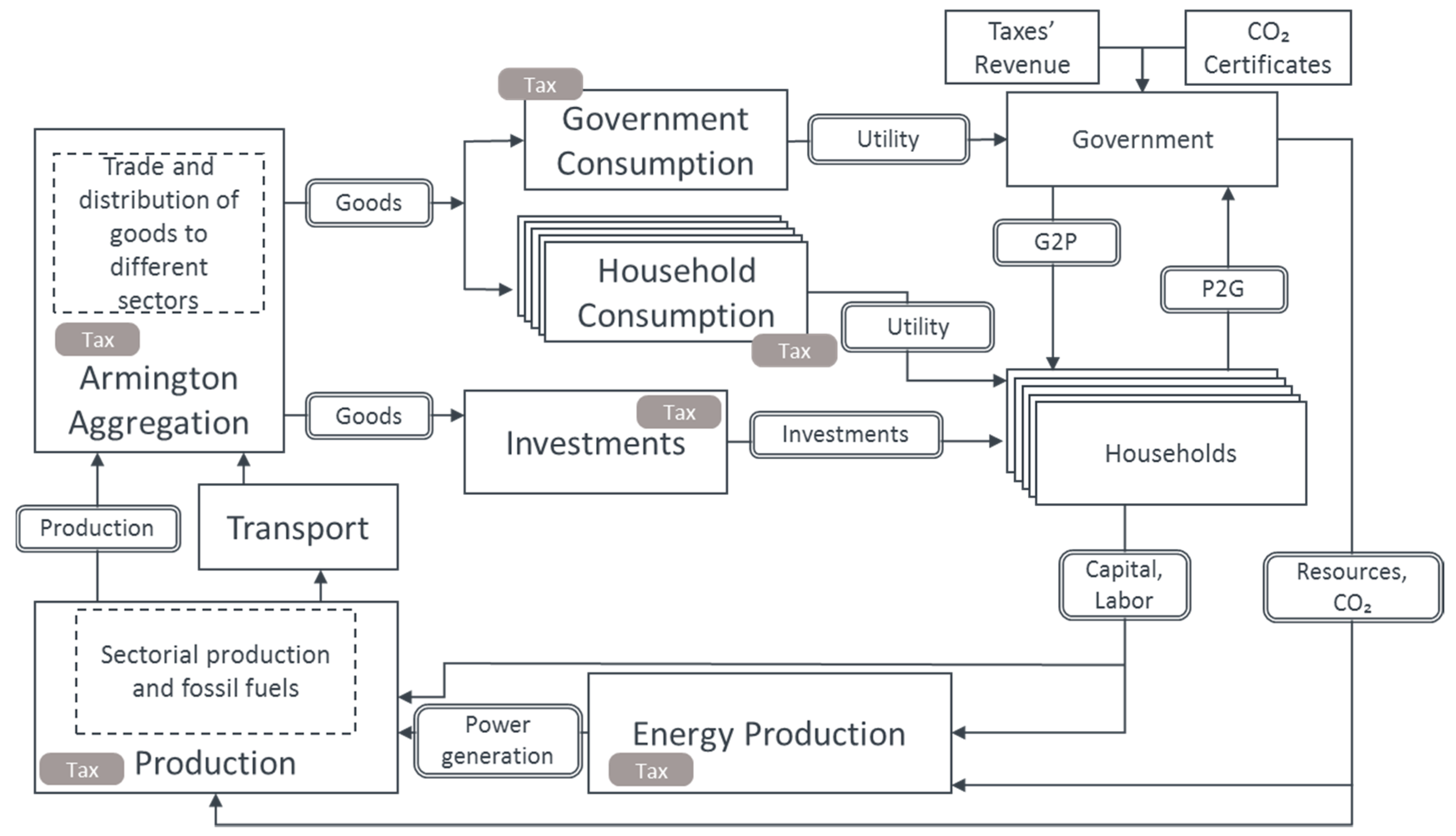
With the implementation of the six blocks representing the government and five income groups, the last step was to add the channels that allow for income flow between these blocks. This flow of income represents the taxation of income, from both labor and capital, from households to the government, and the payment of social benefits and pensions from the government to households. Figure 2 shows a graph of the amended structure of NEWAGE containing a detailed representation of the new process of collecting and distributing tax revenues. The government receives tax revenues, as well as revenues from CO₂ allowances. Income taxes are paid by the households (P2G) and, in return, the government distributes some of the net revenues to the households (G2P) according to the shares that each income group is endowed to receive.

The first data processing step was the calculation of expenditure and income in different household groups of NEWAGE regions. To ensure the confidentiality of respondents and to make our calculations comparable to other datasets, all indicators are calculated at the decile level and, due to project requirements, aggregated to quintiles just before implementation in NEWAGE. To group individuals covered by the dataset to deciles, equivalized disposable income [31] has been calculated by dividing the net income of a household by the equivalized household size (the number of adult equivalents in the household). Equivalized household size has been calculated using a modified OECD scale in which the first adult is equal to 1, the second and each subsequent person aged 14 and over is equal to 0.5, and each child aged under 14 is equal to 0.3. Finally, decile groups were formed taking into account equivalized income, household size, and sample weight.

The same methodology was applied for both SILC and HBS datasets. In the case of the HBS dataset, monetary net income (total monetary income from all sources minus income taxes, EUR_HH095) variable represents households’ disposable income, while for the SILC dataset total disposable household income (HY020) is applied.

The disaggregation of consumption expenditures by deciles was carried out assuming that total expenditure by commodity remains the same as in the aggregated version of NEWAGE. This assumption ensures the consistency of the model that relies on fully balanced GTAP data. Different consumption levels in different deciles were included as proportions of the total consumption expenditure calculated from HBS.

The shares in consumption expenditure on different commodities within each decile suffer mainly from data inconsistency and different classifications: The HBS deals with the classification of individual consumption by purpose (COICOP) [32] categories, while the NEWAGE model uses an aggregated GTAP commodity classification. To gain consistency within the two datasets, a mapping matrix was developed. This matrix maps every commodity in the NEWAGE model with one or more COICOP categories within the HBS dataset. For instance, it is assumed that “oil” in NEWAGE represents “Fuels and lubricants for personal transport equipment” and “Liquid fuels” in the HBS data set. To get a balanced image of consumption structures among decile groups, iterative scaling (an RAS procedure) was performed by fixing total consumption by commodity-based on GTAP data and total consumption expenditure per household decile based on GTAP data on total consumption and consumption shares among deciles obtained from HBS microdata.

Income disaggregation was performed following the income categories represented in the new structure of NEWAGE. For this, we selected the most similar income categories in the SILC survey. In some cases, it was possible to get a rather good fit with the microdata (e.g., for skilled labor income), while in other cases like return on capital, microdata served only as a proxy since the SILC survey covers the income from rental of a property or land and interest, dividends, profit from capital investments in unincorporated business only. To get a more comprehensive and balanced view of income and consumption expenditure, aggregate propensities to consume by income quintile were calculated using HBS microdata. These values were applied as benchmarks with a focus on the poorest quintile and implemented in income disaggregation by using income taxes as a balancing element.

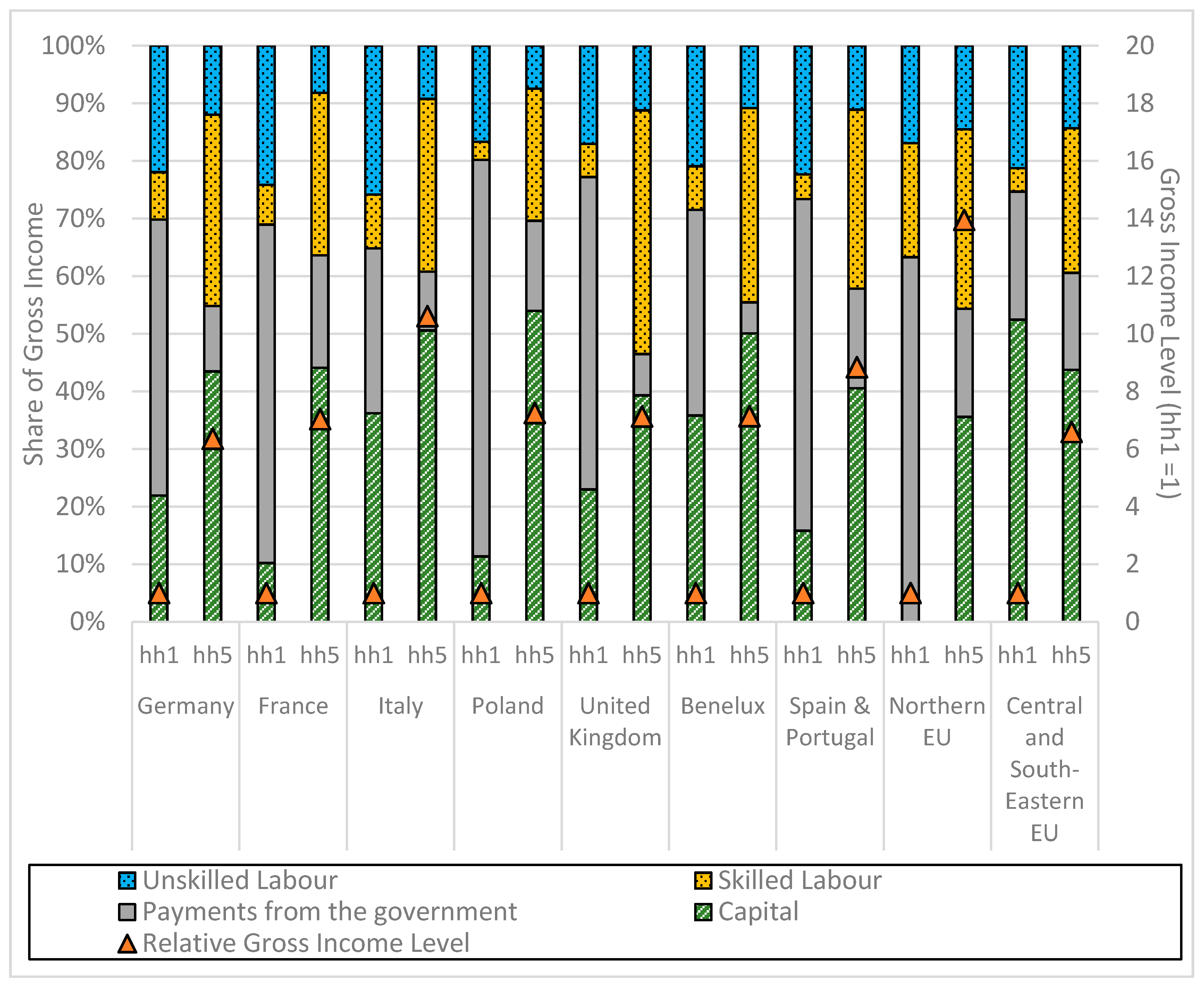
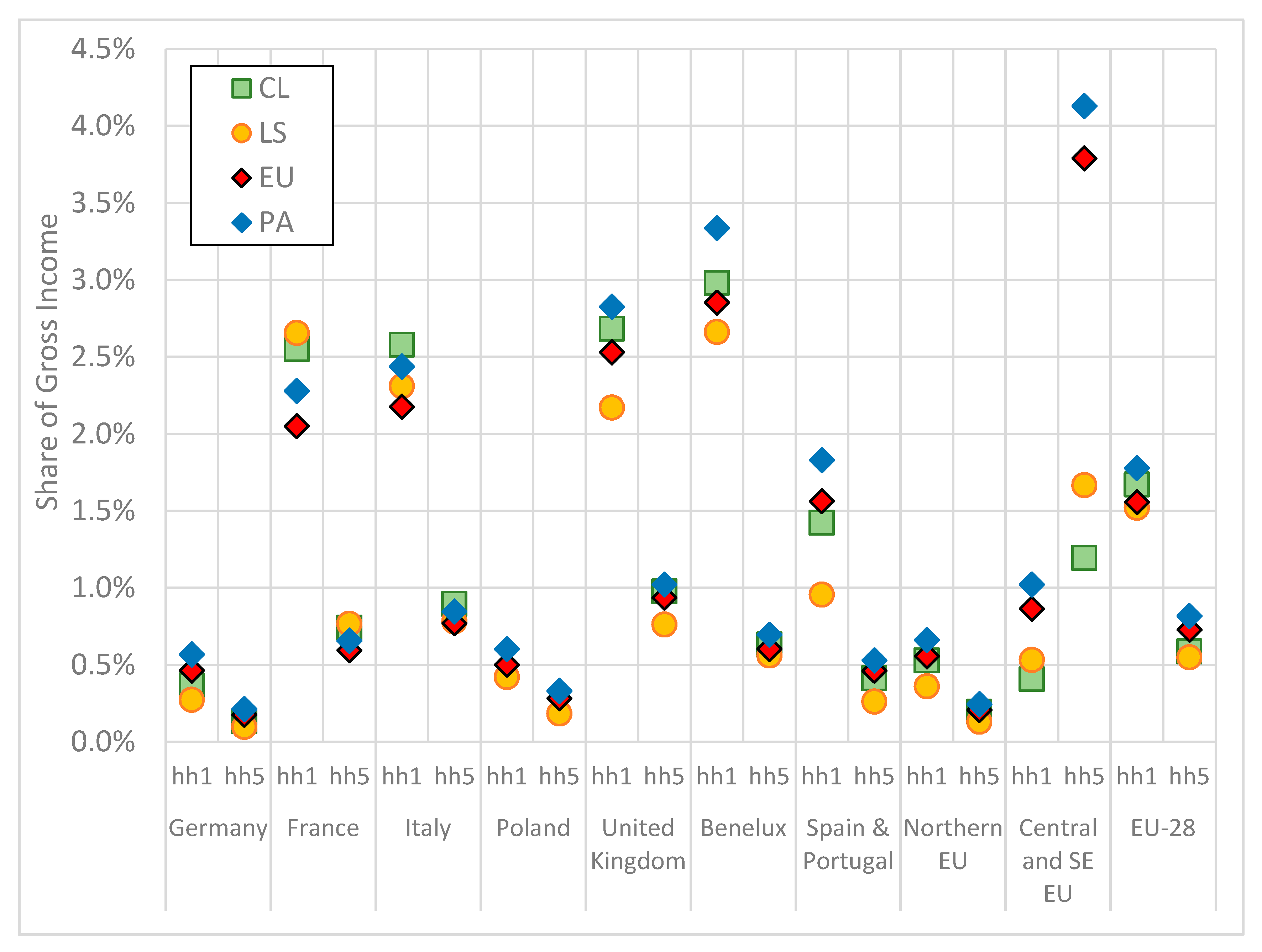
By the end of the disaggregation process, Figure 3 depicts the average composition of the gross income of the five income groups in the EU-28. The figure indicates that the lowest income group has a higher share of gross income from government payments or tax revenues, and the highest income group has the largest share of its gross income from capital revenues, followed by labor payments from skilled labor. Additionally, the regions or countries where the poorest quintile has the highest shares of government payments are the Northern EU, Poland, Spain, and Portugal, i.e., the low-income groups in these regions have the highest potential to benefit from a distribution of revenues from carbon pricing policies.

The disaggregation to quintile groups for each NEWAGE region imposes a methodological issue regarding regions that cover more than one country. This is the case for the region “Central and Eastern Europe”, where the disaggregation into quintile groups within this region means that a household from the lowest income group in the wealthiest country might fall to the highest income group on the regionally aggregated scale. The alternative approach, dealing with country-level income groups within the aggregated region, would result in a diversity of income levels within one group. Despite this disadvantage, we decided for the modeling to keep the actual regional disaggregation in this work, as presented in Table 1, to ensure consistency with previous work conducted in the framework of the REEEM project with NEWAGE, such as [33]. “Northern EU” also represents such a comparable case. Figure 3 depicts the effects of this decision, as it is possible to see that the richest quintile, mostly composed by Sweden and Denmark, has a gross income level roughly 14 times higher than the poorest quintile, mostly composed by the Baltic countries.

3. Results

3.1. Scenarios

There are five distinct scenarios in this work, one reference and four scenario variations, which are applied to analyze the effects of different cap-and-trade strategies on the European economy and its distributional impacts while also considering the influence of factors from outside of the EU-28. The scenarios are classified according to the CO₂ reduction targets within three dimensions: sectors in the EU-28 covered by the actual European Emissions Trading System (EU-ETS) configuration (Power and heat generation, Energy intensive industry (oil refineries, steel, aluminum, etc.) and civil aviation are included in the ETS according to reference [34]), sectors in the EU-28 not covered by the actual EU-ETS configuration, and all sectors or regions outside of the EU-28.

Although formally there is currently one cap-and-trade system in the EU-28 for the sectors covered by the EU-ETS, the other sectors within the EU-28 are modeled as national cap-and-trade systems as well to simplify policy assumptions. The national reduction targets for non-EU-ETS (Residential, commercial, transportation and agriculture are the focus of the Effort Sharing policies according to reference [35]) sectors are set until 2020 according to the Effort Sharing Decision (ESD), and until 2030 according to the Effort Sharing Regulation [35], while for 2050 they are based on specific scenario assumptions, as shown in

Table A7. Emission reduction targets for Coalitions (CL) and Local Solutions (LS) pathways in EU-28.

	Targets for 2020 (Compared to 2005)	Targets for 2030 (Compared to 2005)-Proposal	Target for 2050 (Compared to 2005)-Assumptions
EU-28 ETS	−21%	−43%	−83%
	Effort sharing decision (ESD)	Effort sharing decision (ESD-new)	Effort sharing decision (ESD-new)
France	−14%	−37%	−80%
Portugal	1%	−17%	−80%
Spain	−10%	−26%	−80%
Italy	−13%	−33%	−80%
United Kingdom	−16%	−37%	−80%
Austria	−16%	−36%	−80%
Germany	−14%	−38%	−80%
Netherlands	−16%	−36%	−80%
Belgium	−15%	−35%	−80%
Luxembourg	−20%	−40%	−80%
Austria	−16%	−36%	−80%
Denmark	−20%	−39%	−80%
Sweden	−17%	−40%	−80%
Finland	−16%	−39%	−80%
Ireland	−20%	−30%	−80%
Poland	14%	−7%	−50%
Czech Republic	9%	−14%	−50%
Bulgaria	20%	0%	−60%
Romania	19%	−2%	−60%
Estonia	11%	−13%	−60%
Latvia	17%	−6%	−60%
Lithuania	15%	−9%	−60%
Croatia	11%	−7%	−60%
Hungary	10%	−7%	−60%
Greece	−4%	−16%	−60%
Slovakia	13%	−12%	−60%
Slovenia	4%	−15%	−60%
Cyprus	−5%	−24%	−60%
Malta	5%	−19%	−60%
EU-28	−9%	−30%	−75%

. The regions outside of the EU-28 have specific reduction targets, which are modeled as national (or regional) cap-and-trade systems covering all the sectors of the economy as well. Since official measurements of ETS and non-ETS emissions only started in 2005, reduction targets with sectoral distinctions refer to 2005 as the base year while emission targets without sectoral distinction refer to 1990 as the base year.

The scenarios were developed in the framework of the REEEM project and consider the narratives developed by the white paper on the future of Europe [36].

Table 2. Description of analyzed scenarios.

Coverage	Reference Scenario (REF)	Coalitions Pathway (CL)	Local Solutions (LS)	EU-28 Going Alone (EU)	Paris Agreement (PA)
ETS sectors	62% reduction in 2050 *	83% reduction in 2050 *		95% reduction in 2050 compared to 1990 levels
Non-ETS sectors	No targets	50% to 80% reduction in 2050, see Table A7. Extra European targets: Industry	50% to 80% reduction in 2050, see Table A7. Extra European targets: Residential Transport Services
Non-EU regions	No targets	Norway, Switzerland, Remaining OECD and China: Table A8 Remaining countries: No targets			In line with the 2 °C target

Note: * Compared to 2005 levels.

provides an overview of the scenarios.

3.1.1. Reference Scenario (REF)

REF is a business-as-usual scenario. For CO₂ emissions, emission targets, and GDP within the EU-28, we apply the EU Reference Scenario 2016 [22] as the main data source. The emission figures of the remaining regions are based on the Reference Technology Scenario (RTS) of the Energy Technology Perspectives (ETP) 2017 [37]. In this scenario, we assume a 62% CO₂ emissions reduction target in 2050 compared to 2005 levels for the sectors covered by the EU-ETS and no targets for the remaining sectors, resulting in an overall reduction of CO₂ of 43%. There are no reduction targets for the non-EU-28 regions.

3.1.2. Coalitions (CL) Pathway

The CL Pathway (In other REEEM related publications, this pathway can also be referred to as “Coalitions for a Low Carbon Path”) assumes a more active position of the EU-28 and a few of the remaining regions, however, with different degrees of ambition. In the EU-28, for instance, the overall CO₂ emissions reduction in 2050 is 80% compared to 1990 levels (referring to a 79% reduction compared to 2005), which is reached by two different policies. On the European level, there is an 83% reduction target in 2050 compared to 2005 values for the ETS sectors, while for the remaining sectors national reduction targets are ranging from 50 to 80% resulting in a 75% overall reduction in 2050 compared to 2005 levels. For detailed information regarding the emissions targets, see Table A7.

For the regions outside of the EU-28, the targets are diverse and represent a “Regional Push” scenario. The scenario includes a small group of ambitious regions willing to intensify their efforts decreasing their emissions of GHG. Within this bloc, there are three distinct reduction targets. The first represents regions whose targets are in line with the EU-28 target of reducing 80% of the emissions in 2050 compared to 1990 levels. The second group is formed by the regions willing to reach the necessary emission levels consistent with a 2 °C target and the third group is formed by the regions whose target is the mean average between their current policies and the 2 °C target. For a detailed list of regions that are part of the Regional Push and their targets, see Table A7.

3.1.3. Local Solutions (LS) Pathway

For this scenario, the main assumption is that the primary driver for the energy transition will result from consumers, who will move towards locally generated energy, such as wind turbines and solar panels, due to a sense of urgency towards avoiding climate change. While the ETS and national non-ETS targets remain the same as in the CL pathway, the higher willingness of consumers to produce local and renewable energy is modeled as a tighter emissions cap on the households, and the transportation and commercial sectors.

3.1.4. EU-28 Going Alone (EU) Pathway

This pathway was created to assess the effects on the European economy in case the EU-28 follows the Paris Agreement alone, with a 95% reduction target in 2050 compared to 1990 levels (94.5% compared to 2005), while the remaining regions follow the Regional Push scenario. The objective of this pathway is to enable the assessment of the impacts of higher emission reduction targets on industrial production and consumption in Europe. In this scenario the EU-28 has one cap-and-trade system that covers all the sectors of the economy, which includes not only the EU-ETS sectors, but also residential, transportation, and services.

3.1.5. Paris Agreement (PA) Pathway

Finally, the PA Pathway, as the name suggests, sets the targets for both EU-28 and non-EU-28 regions in line with the commitments signed in the Paris Agreement. More specifically, the emission targets are derived from the 2DS scenario from ETP 2017 [37] defined to limit the rise of global temperature to 2 °C. In this pathway, similar to the previous one, the EU-28 has one cap-and-trade system that covers all the sectors of the economy.

3.2. Gross Domestic Product (GDP)

As the development of the Gross Domestic Product (GDP) is one of the most important economic indicators, the modeled development of this figure for each of the European regions provides a first overview of the changes in the economic situation. To understand the distributional effects, different distributional indicators like the variation in consumer behavior caused by particular policies, the incidence of a carbon price in different income groups, and finally the development of income under each of the scenario variations and REF are shown.

Figure 4 depicts the relative GDP development of the NEWAGE regions inside the EU-28 and the five scenarios between 2011 and 2050 that were analyzed. It shows that, regardless of the scenario, there is positive economic growth in all regions until 2050 and it varies between 30% for Germany in the PA pathway and over 100% for Northern EU in REF. In addition, the average growth in the EU-28 area is the highest for REF at 73%, followed by 67% growth for the EU pathway, 64% for the CL pathway, 62% for the LS pathway and, finally, 55% for PA pathway. These results correspond in principle to the findings of previous studies [10,11,12,13] showing that higher GHG mitigation targets reduce economic growth overall.

Looking more specifically to the scenario variations, we see that the GDP development in the EU pathway is often superior, or at least equal, to the others, although the CO₂ reduction targets for the EU-28 are stricter than in CL or LS pathways. The pattern suggests that maintaining flexibility in distributing the reduction targets to the sectors by submitting all sectors of the economy into one single cap-and-trade scheme is more cost-effective than keeping individual targets for the different sectors as in CL and LS. Furthermore, the PA pathway reveals a significantly lower GDP development in comparison to the EU pathway, although the same strict targets apply for EU-28 in both scenarios. While the European economy becomes more competitive when the other regions of the world follow stricter emission targets, these regions also have to invest more in CO₂ emission abatement measures which decreases their consumption of European produced goods and, as the net effect, end up reducing both European industrial production and GDP growth.

When comparing the CL and LS pathways only, the results show CL to have a higher average GDP development in the EU-28, increasing 64% in 2050 compared to a 62% increase in LS. However, when analyzing specific regions, the same is true for three regions only: Poland, Spain and Portugal, and Central and Southern EU. These results are due to the lower reduction targets on the CL pathway for non-ETS sectors in Poland as well as Central and South-Eastern EU, causing higher GDP growth in this case in these regions. Regarding Spain and Portugal, this happened because the industrial production in this region is lower than in other western European regions and corresponds to 22% of total GDP, while services correspond to 75% [38]. Therefore, its GDP is less affected by the policy portfolio from the CL pathway, which has stricter targets for industry, than by the LS pathway. For comparison, the contribution of the industry for Germany’s GDP is 30.7% and services is 68.6% [38].

The results shown in Figure 4 suggest also that GDP development depends not only on policies but also on the region that is analyzed. Two factors being specific to each region help to explain this behavior: technology development and labor force growth. While the first factor is connected to the ability of companies producing goods requiring fewer resources as time goes on, the second factor is directly connected to the endowment of labor in each region and plays a major role in the regional GDP development. For instance, according to reference [28], Germany is supposed to have one of the lowest growth rates of the labor force in the EU-28, in contrast to the Northern EU with one of the highest. This explains why the first region has a lower GDP growth in the long-term compared to the second. More details regarding the main drivers of economic growth in REF are available in reference [22].

3.3. Share of Consumption Dedicated to Energy Goods

It is expected that CO₂ cap-and-trade policies will increase the final price of fossil fuels paid by households and, in return, increase the consumption of electricity because CO₂ emitting technologies will be penalized with a higher price on their emissions. Therefore, we analyze the impact of such a policy in the four different scenario variations by showing how the consumption of energy goods changes over time. The definition of energy goods in this work aligns itself with the sectoral disaggregation of NEWAGE and covers the following energy carriers: coal, oil products (including heating and transportation), natural gas, and electricity. Additionally, the respective carbon price paid for each fossil fuel is also included in the calculation of energy goods.

Figure 5 depicts the change in the consumption of fossil fuels for each European region in NEWAGE between 2011 and 2050 for the lowest and highest income groups. It shows that in the EU-28 there is, on average, a higher decrease in fossil fuel consumption in the lowest income groups. Additionally, there is a tendency for this consumption to decrease in every scenario and every region, while the only exceptions are for France and the United Kingdom for REF because in these cases, there is an increase of fossil fuel consumption. This effect can be explained due to an already low share of consumption of fossil fuels in the UK and France in 2011 followed by a high increase in gross income in 2050, as shown in Figure 10a. In effect, these countries have the third and second highest income growth, respectively, which then encourages a higher consumption of fossil fuels.

In Figure 5, the effect of carbon pricing can also be perceived as the reduction in consumption is higher for the scenario variations (CL, LS, EU, PA), except for the CL pathway in Poland due to the low reduction targets of this region in this specific scenario.

The linkage between fossil fuel consumption and carbon pricing can be better perceived in Figure 6 where the share of total consumption dedicated to carbon payments is plotted against the difference in the change of fossil fuel consumption compared to REF for the lowest and highest income groups. This picture shows that as the share of carbon payments increases, the consumption of fossil fuel compared to REF decreases. Additionally, the results indicate that regions with highest fossil fuel reduction in REF, such as Germany, Poland, and Northern EU (see Figure 5), tend to dedicate the lowest share of income to carbon payments because the reduction in fossil fuel consumption is achieved through technology development, as shown in reference [22].

On the other hand, regions with the lowest reduction of fossil fuel consumption in REF, such as France and the UK, have to dedicate a higher share of their consumption towards carbon payments.

In parallel to the consumption of fossil fuels shown in Figure 5, Figure 7 depicts the variation in consumption of electricity in the EU-28 between 2011 and 2050. On average, the highest income group has a higher increase on their consumption of electricity than the low-income groups, with the lowest increase being for REF and the highest for the EU pathway. Just as in Figure 5, the effects are strongly dependent on the region and it is possible to see the effects of the carbon price because all the scenario variations (CL, LS, EU, PA) produce a higher consumption of electricity than REF. Additionally, the results indicate electrification of the energy consumption in the household sector, where the reduction of fossil fuel consumption goes in line with an increase in the electricity consumed.

The share of consumption dedicated to energy goods for the richest and poorest income quintiles in the EU-28 can be seen in Figure 8. To create this figure, we calculated the average share of energy goods in total consumption for each of the nine regions in the NEWAGE model and each income group in 2011 and 2050. It is important to note that all scenarios utilize the same technology development assumptions and the higher shares of energy goods in consumption in the scenario variations (CL, LS, EU, PA) compared to REF arise from both carbon payments and substitution of fossil fuels for electricity, which outweighs the lower consumption of fossil fuels.

The results indicate that in 2011, the average share of total consumption for energy goods in the EU-28 varied between 6.8% in the lowest income group (hh1) and 5.9% in the highest income group (hh5). In 2050 the share of energy goods decreases in every scenario for all income groups and varies between 3.9% in REF and 5.4% in the PA pathway for the lowest income groups (hh1) and between 3.1% in REF and 4.8% in the PA pathway for the highest income group (hh5).

As for specific regions, the results indicate that most of them follow the EU-28 average numbers where the share to be spent on energy reduces for all households in all of the scenarios. Even with this reduction, lower-income households still have to spend a higher share of their consumption on energy goods in 2050. Additionally, the largest reduction in the consumption share of energy goods for the lowest income group (hh1) and the highest income group (hh5) are seen on the REF since there are no carbon payments. It is also possible to perceive a connection with the reduction in fossil fuel consumption, as shown in Figure 5, because the regions that managed to reduce the most fossil fuel consumption in the REF for 2050, such as Germany, Northern EU, and Poland, also have the highest reductions in the share of consumption dedicated to energy goods in all scenarios. On the other hand, regions such as the UK and France, with a higher consumption of fossil fuels for REF in 2050, have similar consumption levels of energy goods for the scenario variations (CL, LS, EU, PA) in 2050 compared to 2011 levels.

Another tendency that remains true for most regions is that the consumption shares of energy goods between 2011 and 2050 decrease for all scenarios. The few cases this does not apply to are France, the UK, and Central and South-Eastern EU. For the first two regions, this effect was already discussed above. However, for Central and South-Eastern EU, the consumption shares of energy goods do not reduce for the richest income group (hh5) in both EU and PA pathways between 2011 and 2050, because this group reveals one the highest increases in electricity consumption, shown in Figure 7, and pay the highest shares of consumption for carbon payments, as shown in Figure 6. Therefore, this group maintains a level of consumption share dedicated to energy goods that is nearly unchanged in these two scenarios with a different mix of energy carriers. Nevertheless, it should be noted, that due to the modeling restrictions for Central and South-Eastern EU explained in Section 2, this result might be limited in significance as there are significant disparities within the income groups in the region and the countries represented by the region.

3.4. Incidence of Carbon Pricing in Different Income Groups

Figure 9 shows the share of gross income to be spent on carbon prices on average for the highest and lowest income groups in the NEWAGE regions of EU-28, as well as the aggregated EU-28. The tendency in the EU-28 (right end of Figure 9) is that groups with lower income have to spend a higher share of their income for carbon payments than groups with higher income. Due to the above-mentioned reasoning, that behavior cannot be depicted in the diverse region of Central and South-Eastern EU. Additionally, the results show that while the variation on share of gross income spent on carbon payments is much higher for low-income households, varying between 0.5% for Germany and Northern EU to around 3% for Benelux, the variation for the group with the highest incomes ranges between 0.2% for Germany and Northern EU to 1% for the UK, with Central and South-Eastern EU being an outlier in this case by getting up to 4% for the PA pathway. In summary, this indicates that low-income households are more vulnerable to carbon pricing policies because the range of the variation is higher for them.

It is worth noting that the regions with the lowest decrease in fossil fuel consumption in REF for 2050, as shown in Figure 5, also present the highest shares of income dedicated to the payment of carbon prices. Examples for this case are France, Italy, the UK, and Benelux. At the same time, regions that managed to reduce fossil fuel consumption in REF also tend to use a lower share of their gross income to pay for carbon prices, as in Germany, Poland, and the Northern EU.

3.5. Income Development for Different Income Groups

Figure 10a depicts the development of average gross income across all income groups, where the values are shown relative to 2011. The results indicate that the development of gross income is similar to the growth of GDP for the counterfactual scenarios (CL, LS, EU, PA), indicating higher income growth for the EU pathway as it presents high GDP growth as well, followed by the LS pathway, the CL pathway, and finally the PA pathway. In some cases, such as for Germany, Poland, the Northern EU, and Central and South-Eastern EU, the growth of gross income in the EU pathway even surpasses the growth in REF due to the extra revenue from carbon payments being added to the income of households. In these cases, income also grows more than GDP itself, which can be explained by a higher level of consumption, which positively influences GDP, followed by an increase in imports, which negatively affects GDP. For more details about the growth of different components of GDP, consult

Table A9. Level of GDP components in 2050 (2011 = 100%). In NEWAGE, GDP is the sum of Government’s consumption (1), Households’ consumption (2), Investments (3) and Exports (4) minus Imports (5).

Region	Scenario	1	2	3	4	5	Total GDP
Germany	REF	159.40%	151.57%	152.00%	165.02%	185.73%	145.70%
	CL	154.35%	149.48%	147.75%	157.03%	183.02%	140.38%
	LS	155.90%	149.94%	148.31%	159.63%	184.13%	141.72%
	EU	159.39%	158.43%	153.45%	148.65%	185.47%	143.15%
	PA	141.83%	144.84%	138.73%	144.92%	175.79%	131.23%
France	REF	157.21%	175.58%	175.20%	227.86%	201.71%	176.87%
	CL	150.36%	164.71%	160.13%	197.68%	187.87%	162.02%
	LS	153.73%	167.81%	162.90%	188.32%	188.90%	162.52%
	EU	156.07%	167.42%	165.32%	208.62%	187.05%	169.12%
	PA	141.63%	156.26%	153.02%	215.72%	186.09%	158.67%
Italy	REF	146.72%	156.23%	156.47%	198.93%	193.21%	155.20%
	CL	140.85%	148.72%	145.58%	181.14%	188.98%	143.67%
	LS	143.31%	151.31%	148.29%	183.64%	190.14%	146.64%
	EU	146.42%	154.21%	151.71%	180.76%	183.42%	150.89%
	PA	128.34%	139.48%	135.73%	173.48%	171.74%	136.35%
Poland	REF	225.70%	177.75%	202.12%	243.11%	211.38%	201.94%
	CL	218.42%	169.45%	190.87%	250.48%	211.38%	195.43%
	LS	222.40%	176.55%	195.56%	220.06%	203.96%	193.77%
	EU	229.44%	204.57%	203.29%	183.84%	222.52%	193.73%
	PA	205.65%	187.41%	184.80%	184.34%	214.49%	177.62%
UK	REF	180.04%	198.29%	208.54%	280.48%	240.01%	203.81%
	CL	170.82%	190.20%	188.82%	248.65%	226.04%	189.22%
	LS	172.40%	190.51%	190.05%	246.18%	223.01%	190.34%
	EU	178.33%	195.63%	195.49%	250.45%	225.58%	196.33%
	PA	155.43%	179.97%	175.01%	250.18%	216.72%	180.13%
Benelux	REF	184.03%	181.88%	186.80%	196.75%	201.89%	180.41%
	CL	175.30%	177.57%	170.01%	174.48%	190.27%	166.31%
	LS	177.78%	182.59%	173.21%	170.79%	189.03%	168.90%
	EU	181.53%	180.26%	175.47%	174.88%	190.90%	170.47%
	PA	162.47%	165.75%	158.33%	177.31%	184.33%	159.12%
Spain + Portugal	REF	170.95%	153.25%	157.69%	227.87%	193.69%	165.39%
	CL	163.58%	151.07%	151.27%	192.10%	180.56%	155.75%
	LS	160.72%	146.48%	147.38%	171.14%	173.39%	148.21%
	EU	165.55%	152.36%	152.26%	178.35%	178.30%	154.29%
	PA	150.05%	141.16%	140.06%	186.84%	178.09%	143.80%
Northern EU	REF	193.52%	224.64%	221.85%	224.21%	251.81%	205.62%
	CL	190.32%	220.39%	217.99%	214.03%	244.43%	200.20%
	LS	195.58%	223.70%	221.92%	207.32%	242.40%	201.60%
	EU	194.66%	227.11%	224.11%	208.02%	243.96%	203.20%
	PA	174.24%	208.03%	204.71%	211.38%	239.72%	188.21%
CSE EU	REF	172.88%	154.31%	153.36%	230.56%	192.88%	172.30%
	CL	172.95%	156.81%	156.27%	239.94%	198.53%	175.97%
	LS	168.22%	155.07%	154.56%	180.65%	179.60%	157.06%
	EU	173.38%	159.86%	159.49%	200.41%	190.81%	165.40%
	PA	161.47%	151.52%	151.03%	216.71%	193.91%	161.72%

.

Figure 10b depicts the difference of relative growth between the lowest (hh1) and highest (hh5) income groups for all EU-28 regions in NEWAGE, where positive numbers indicate that the income of the lowest-income households (hh1) grow more than the highest-income households (hh5) and vice versa. For instance, results for REF indicate that between 2011 and 2050, gross income in Germany will grow by 45.6% for the lowest income group and 49.8% for the highest income group, which accounts for a growth difference of −4.3%, as shown in Figure 10b.

The results indicate that the regional average, as shown by the EU-28 values, is that the richest households have a higher growth of gross income with the less strict energy policies of REF, although GDP grows higher in this case. The only case where the poorest households have a higher growth of gross income for REF is in the Northern EU, because the countries within this region already have strong income transfer policies which can be explained by the high-income tax rates, especially in Sweden, Denmark, Finland, and Ireland [39], and a high share of government payments as part of gross income in the low-income group, as shown inFigure 3. As for the scenario variations, the EU and PA pathways usually lead to higher income growth of the poorest households due to the transfer of income that is happening through the carbon payments. Even when the income of the lowest-income group (hh1) does not grow more than the highest-income group (hh5), at least the difference between the two income groups decreases when compared to REF, as can be seen in Poland, the UK, Spain and Portugal, and Central and South-Eastern EU.

4. Discussion

The results indicate the existence of a trade-off between CO₂ reduction and economic growth, as described in references [9,10,11,12,13] due to the GDP level of the scenario variations in 2050 being lower than REF, as seen in Figure 4. Additionally, the results indicate that the selected cap-and-trade scheme is an important factor for economic growth, as the EU pathway presents a higher GDP level in the EU-28 than the other scenario variations, despite resulting in lower CO₂ emissions. Another factor that influences the economic output is the commitment of countries outside of the EU-28 to reduce their emissions because the PA pathway always presented lower GDP values than the EU pathway, despite having the same cap-and-trade scheme, suggesting that decreasing CO₂ emissions in non-EU-28 regions reduce their demand for European goods and therefore lowers the European GDP.

Regarding the distributional impacts, it was shown that the carbon price paid by different income groups is regressive, as also indicated by reference [16], meaning that the share of income dedicated to the carbon payments decreases as income increases. This indicates, that poorer households will have a higher propensity to reduce their emissions than richer as the carbon price will constitute a higher share of their budget. On the other hand, the results demonstrate that redistributing the revenues from carbon certificates in the same proportion that payments from government to households are made today to various income quintiles can work as a tool to decrease income inequality, as shown in references [15,17], because the poorer households derive a higher share of their income from government payments and would, therefore, observe higher gross income growth than richer households.

5. Conclusions

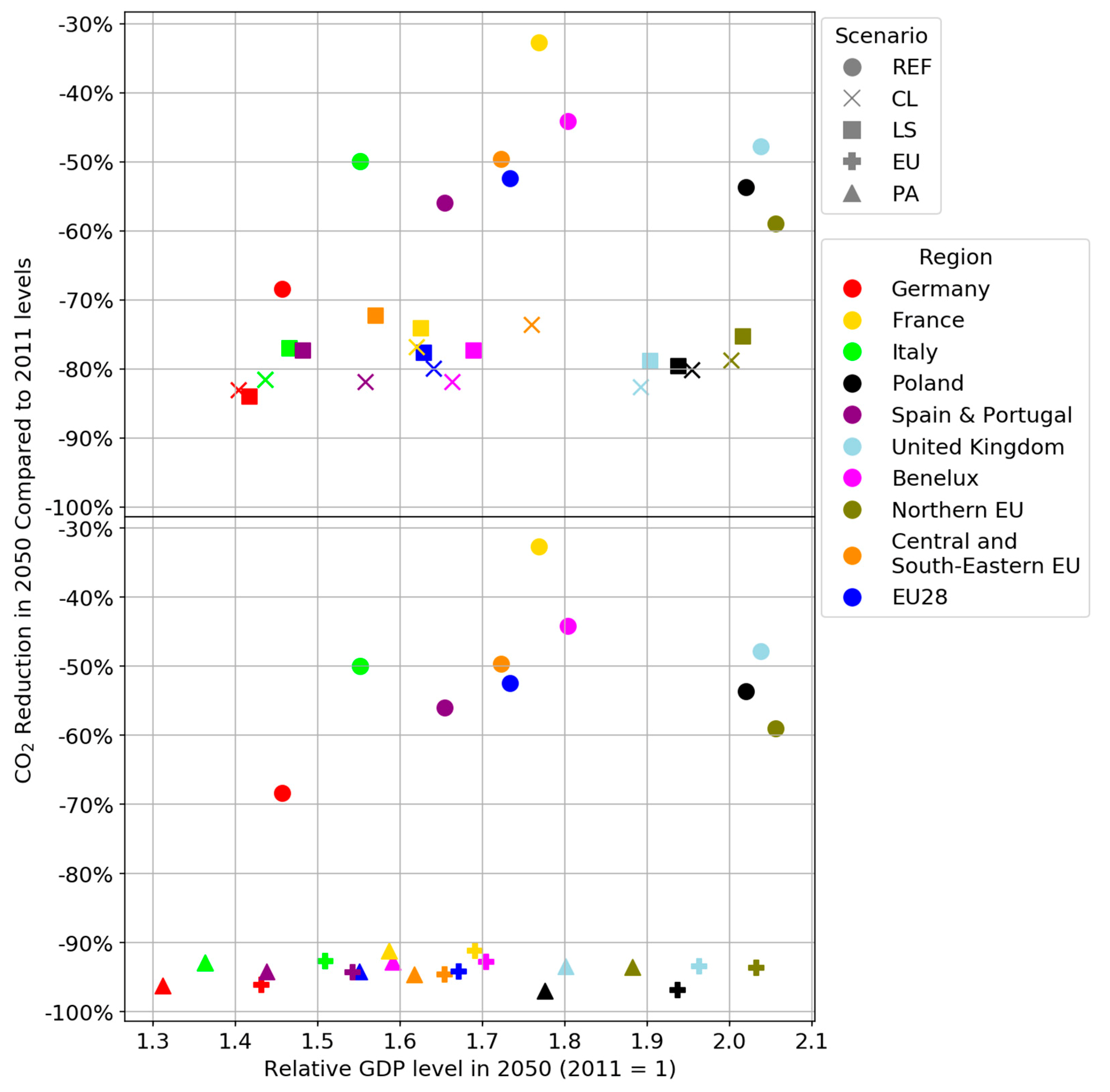
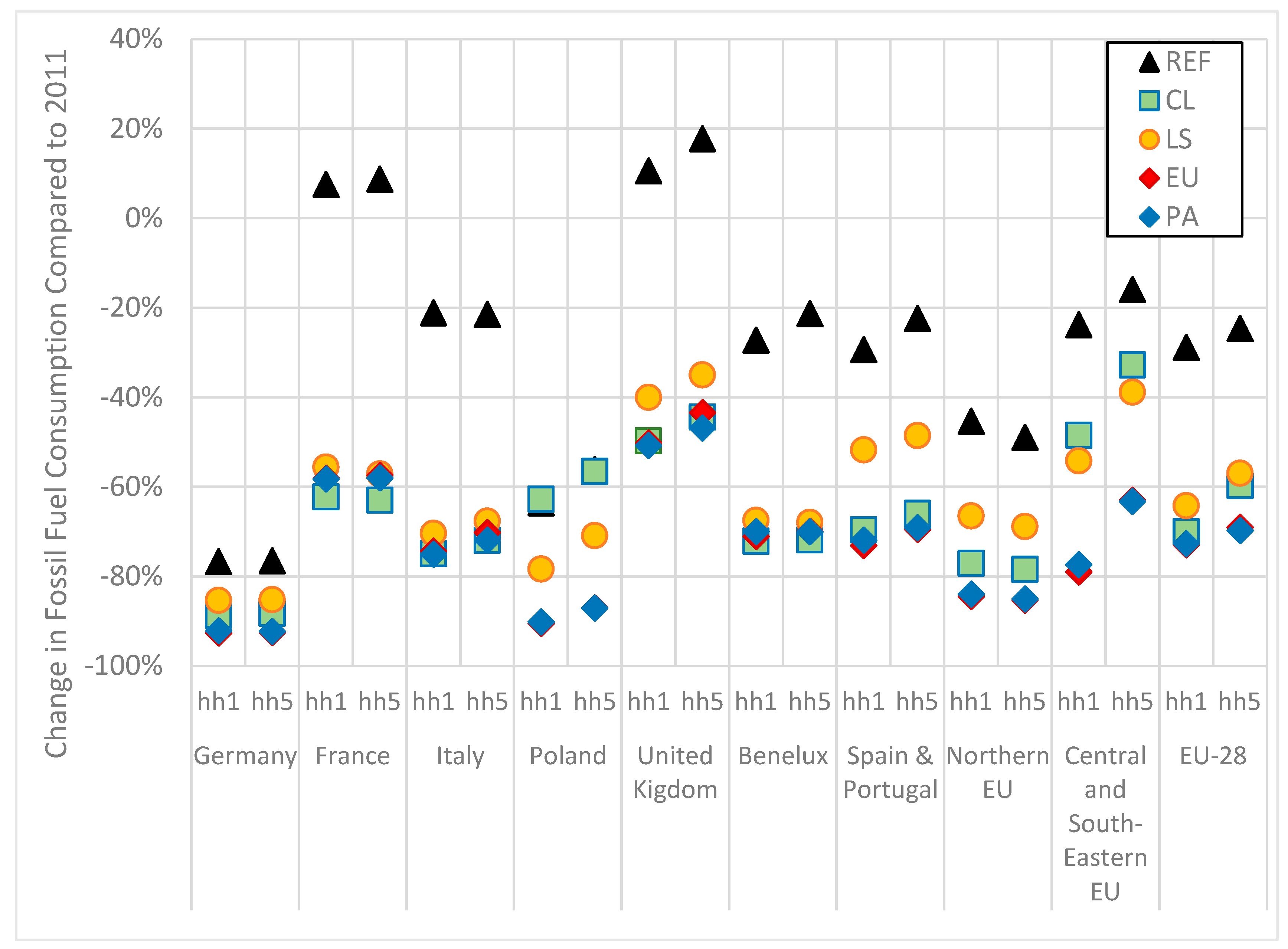
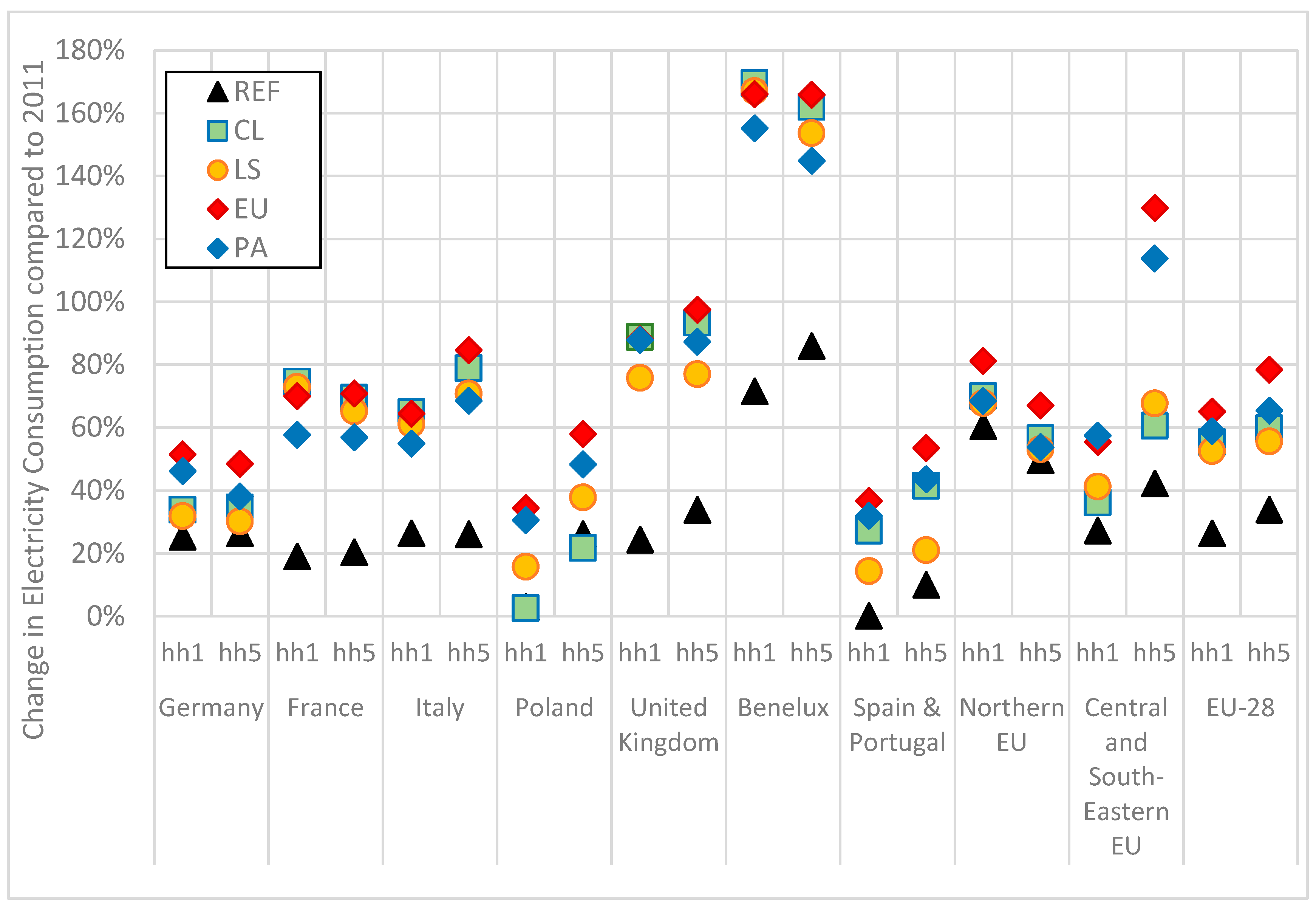
Throughout this work, different effects of energy policies based on the cap-and-trade system were analyzed by different parameters, namely GDP growth, consumption of energy goods, the incidence of a carbon price, and the development of income. The analysis was based on a reference scenario and four scenario variations: Coalitions (CL), Local Solutions (LS), EU-28 Going Alone (EU), and Paris Agreement (PA) pathways. They differed between one another in aspects such as sectoral coverage of carbon cap-and-trade scheme, reduction targets for 2050 and international cooperation against climate change. Additionally, the NEWAGE model had to be further developed to account for income quintiles and be able to assess the effects that carbon pricing has over consumption and income development for different income groups in multiple regions.

The results indicate the existence of a trade-off between economic growth and CO₂ reduction and identified the cap-and-trade scheme and international commitment to reduce CO₂ as key drivers for economic development. More specifically, a European cap-and-trade system where all the sectors of the economy are included produces a higher economic output for the majority of regions in the EU-28 and the higher the commitment of non-EU-28 to reduce their emissions, the lower their capacity to import European goods.

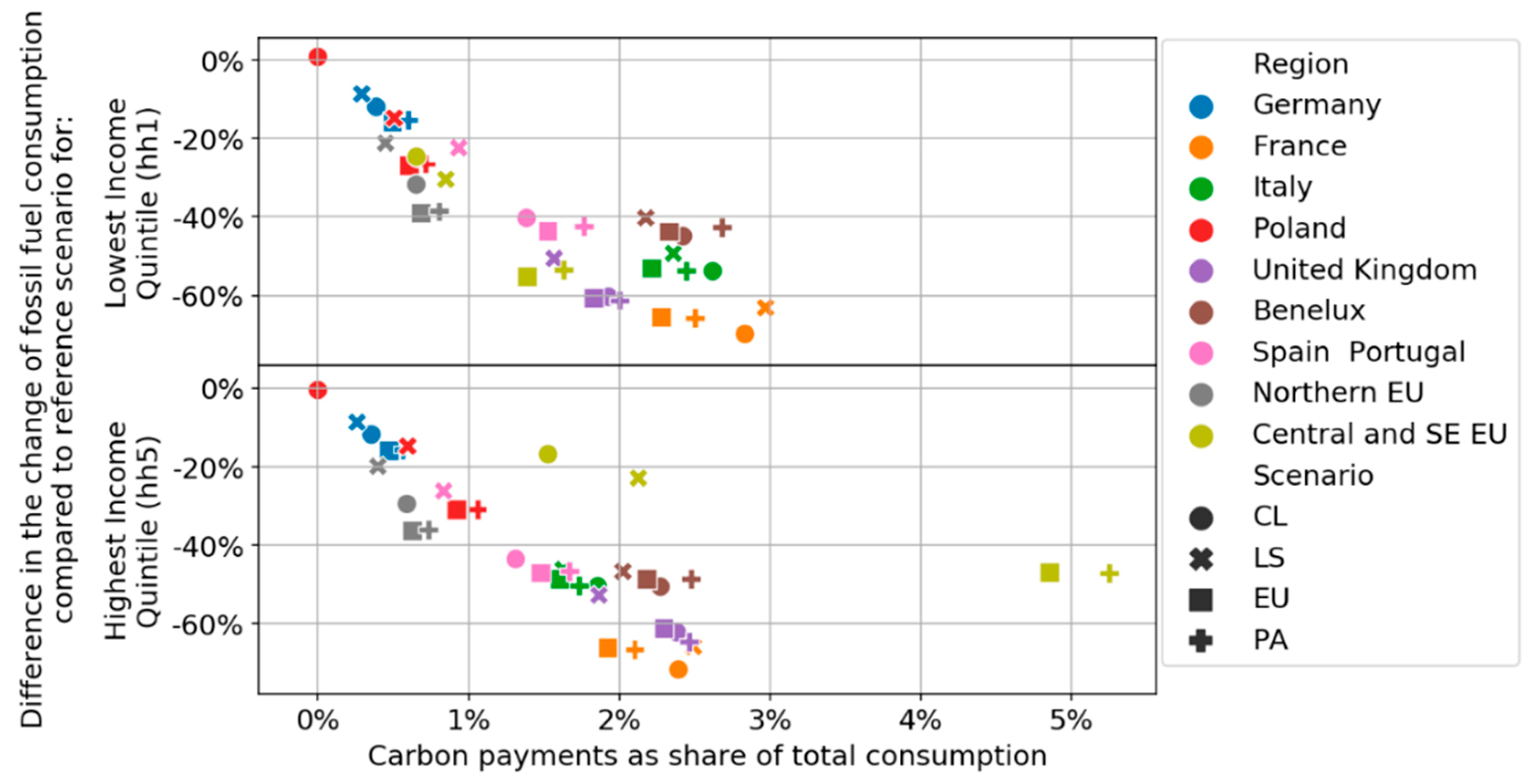
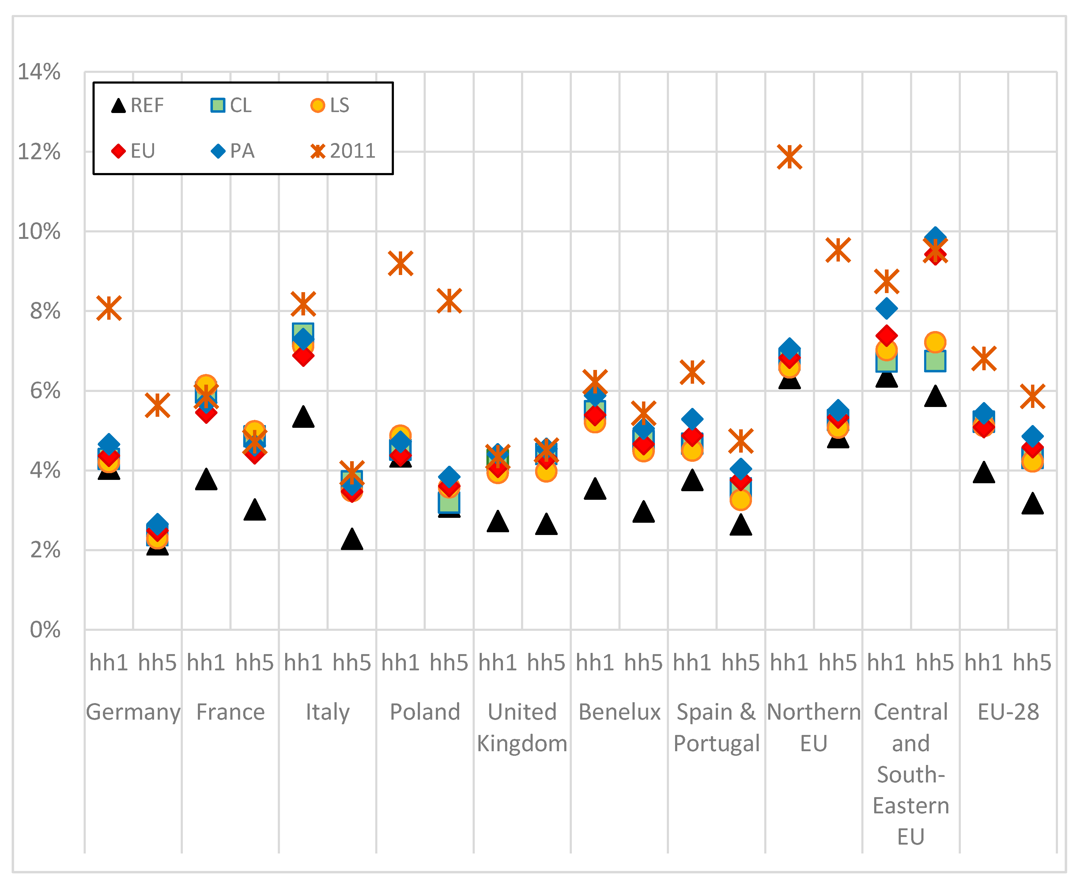
Additionally, it demonstrated that the cap-and-trade schemes analyzed in this work are regressive, but the one presented in EU and PA pathways provide an income increase for low-income households. These findings are relevant for the acceptance of carbon pricing measures in the household sector because they show that poorer households can obtain financial benefits from such energy policies when the revenue is redistributed to households and, as shown by Carattini et al. [40], the proposed strategies to redistribute the revenues from such policies play a key role in obtaining voter acceptance.

As for future research based on the questions raised by this work, there are a few aspects that should be further studied. First, as non-European countries have a major influence over the economic development of the European economy, the development of different pathways regarding environmental policies implemented outside of the EU-28 and how to respond to them appropriately is especially important in a time of political instability and disagreements with countries such as the United States, Russia, and China. Secondly, it is crucial for a better understanding of the real impacts of policies to internalize environmental gains and losses as the costs of environmental measures, or lack thereof, would be more clearly perceived in economic parameters such as GDP and trade balances. Third, an aspect of the energy transition that could not be analyzed in detail is the level of investments made by households in energy efficiency. In the present version of NEWAGE, households can only substitute their fossil fuel consumption directly for electricity. Future work should expand their options to allow for direct investment in different technologies that decrease their energy consumption. Finally, this report considered that all pathways would have the same revenue recycling scheme for the carbon payments and, as it was shown that redistributing this revenue to households can have positive effects on diminishing income inequality, establishing new recycling schemes with a focus on low-income households and the substitution of existing taxes, such as on labor and capital, with environmental taxes through an ETR should be further studied.

References

1. Intergovernmental Panel on Climate Change (IPCC). AR5 Synthesis Report; IPCC: Geneva, Switzerland, 2014; Available online: https://www.ipcc.ch/report/ar5/syr/ (accessed on 14 September 2019).
2. United Nations Framework Convention on Climate Change. The Paris Agreement. Available online: https://unfccc.int/process-and-meetings/the-paris-agreement/the-paris-agreement (accessed on 14 September 2019).
3. Nordhaus, W.D. Geography and macroeconomics: New data and new findings. Proc. Natl. Acad. Sci. USA 2006, 103, 3510–3517. [Google Scholar] [CrossRef] [PubMed] [Green Version]
4. Horowitz, J.K. The income–temperature relationship in a cross-section of countries and its implications for predicting the effects of global warming. Environ. Resour. Econ. 2009, 44, 475–493. [Google Scholar] [CrossRef]
5. Hsiang, S.M. Temperatures and cyclones strongly associated with economic production in the Caribbean and Central America. Proc. Natl. Acad. Sci. USA 2010, 107, 15367–15372. [Google Scholar] [CrossRef] [PubMed] [Green Version]
6. Dell, M.; Jones, B.F.; Olken, B.A. Temperature shocks and economic growth: Evidence from the last half century. Am. Econ. J. Macroecon. 2012, 4, 66–95. [Google Scholar] [CrossRef] [Green Version]
7. Burke, M.; Hsiang, S.M.; Miguel, E. Global non-linear effect of temperature on economic production. Nature 2015, 527, 235–239. [Google Scholar] [CrossRef] [PubMed]
8. Lemoine, D.; Kapnick, S. A top-down approach to projecting market impacts of climate change. Nat. Clim. Chang. 2016, 6, 51–55. [Google Scholar] [CrossRef]
9. Adams, P.D. Insurance against catastrophic climate change: How much will an emissions trading scheme cost Australia? Aust. Econ. Rev. 2007, 40, 432–452. [Google Scholar] [CrossRef] [Green Version]
10. Adams, P.D.; Parmenter, B.R.; Verikios, G. An emissions trading scheme for Australia: National and regional impacts. Econ. Rec. 2014, 90, 316–344. [Google Scholar] [CrossRef] [Green Version]
11. Lu, C.; Tong, Q.; Liu, X. The impacts of carbon tax and complementary policies on Chinese economy. Energy Policy 2010, 38, 7278–7285. [Google Scholar] [CrossRef]
12. Guo, Z.; Zhang, X.; Zheng, Y.; Rao, R. Exploring the impacts of a carbon tax on the Chinese economy using a CGE model with a detailed disaggregation of energy sectors. Energy Econ. 2014, 45, 455–462. [Google Scholar] [CrossRef]
13. Fragkos, P.; Tasios, N.; Paroussos, L.; Capros, P.; Tsani, S. Energy system impacts and policy implications of the European Intended Nationally Determined Contribution and low-carbon pathway to 2050. Energy Policy 2017, 100, 216–226. [Google Scholar] [CrossRef]
14. Goulder, L.H. Climate change policy’s interactions with the tax system. Energy Econ. 2013, 40, S3–S11. [Google Scholar] [CrossRef]
15. Caron, J.; Cole, J.; Goettle, R.; Onda, C.; Mcfarland, J.; Woollacott, J. Distributional implications of a national CO2 tax in the U.S. cross income classes and regions: A multi-model overview. Clim. Chang. Econ. 2018, 9, 1840004. [Google Scholar] [CrossRef] [Green Version]
16. Reaños, M.T.; Lynch, M.Á. Carbon Taxation in Ireland: Distributional Effects of Revenue Recycling Policies; Economic and Social Research Institute (ESRI): Dublin, Ireland, 2019; Available online: https://www.esri.ie/publications/carbon-taxation-in-ireland-distributional-effects-of-revenue-recycling-policies (accessed on 14 September 2019).
17. Tran, T.M.; Siriwardana, M.; Meng, S.; Nong, D. Impact of an emissions trading scheme on Australian households: A computable general equilibrium analysis. J. Clean. Prod. 2019, 221, 439–456. [Google Scholar] [CrossRef]
18. Maxim, M.R.; Zander, K. Can a green tax reform entail employment double dividend in European and non-European countries? A survey of the empirical evidence. Int. J. Energy Econ. Policy 2019, 9, 218–228. [Google Scholar] [CrossRef]
19. Freire-González, J.; Ho, M.S. Carbon taxes and the double dividend hypothesis in a recursive-dynamic CGE model for Spain. Econ. Syst. Res. 2019, 31, 267–284. [Google Scholar] [CrossRef]
20. Streimikiene, D.; Siksnelyte, I.; Zavadskas, E.; Cavallaro, F. The impact of greening tax systems on sustainable energy development in the Baltic States. Energies 2018, 11, 1193. [Google Scholar] [CrossRef] [Green Version]
21. Bouet, A.; Estrades, C.; Laborde, D. Households Heterogeneity in a Global CGE Model: An Illustration with the MIRAGE-HH (MIRAGE-HouseHolds) Model; Laboratoire d’Analyse et de Recherche en Economie et Finances Internationales (LAREFI): Pessac, France, 2013. [Google Scholar]
22. Capros, P.; De Vita, A.; Tasios, N.; Siskos, P.; Kannavou, M.; Petropoulos, A.; Evangelopoulou, S.; Zampara, M.; Papadopoulos, D.; Nakos, C.; et al. EU Reference Scenario 2016: Energy, Transport and GHG Emissions—Trends to 2050; Publications Office of the European Union: Luxembourg, 2016; ISBN 978-92-79-52374-8. [Google Scholar]
23. Korkmaz, P.; Blesl, M.; Fahl, U.; Balyk, O.; Petrović, S.; Simonsen, M.B.; Henke, H. REEEM-D6.1_Integrated Energy System Model; REEEM Project: Stockholm, Sweden, 2019. [Google Scholar] [CrossRef]
24. Beestermöller, R. Die Energienachfrage Privater Haushalte und Ihre Bedeutung für den Klimaschutz : Volkswirtschaftliche Analysen zur Deutschen und Europäischen Klimapolitik mit Einem Technologiefundierten Allgemeinen Gleichgewichtsmodell; Universität Stuttgart: Stuttgart, Germany, 2017. [Google Scholar]
25. Montenegro, R.C.; Fahl, U. Carbon leakage and competitiveness: Socio-economic impacts of greenhouse gas emissions decrease on the European area until 2050. In Proceedings of the 2017 14th International Conference on the European Energy Market, Dresden, Germany, 6–9 June 2017; pp. 1–5. [Google Scholar]
26. Aguiar, A.; Narayanan, B.; McDougall, R. An overview of the GTAP 9 data base. J. Glob. Econ. Anal. 2016, 1, 181–208. [Google Scholar] [CrossRef]
27. International Energy Agency. Electricity Information 2013; Electricity Information; OECD: Paris, France, 2013; ISBN 978-92-64-20308-2. [Google Scholar]
28. Fouré, J.; Bénassy-Quéré, A.; Fontagné, L. The Great Shift: Macroeconomic Projections for the World Economy at the 2050 Horizon; Centre d’Études Prospectives and d’Informations Internationales (CEPII): Paris, France, 2012. [Google Scholar]
29. Eurostat. HBS Household Budget Survey Microdata. Survey 2010; Eurostat: Brussels, Belgium, 2017. [Google Scholar]
30. Eurostat. EU-SILC European Union Statistics on Income and Living Conditions Microdata; Eurostat: Brussels, Belgium, 2017. [Google Scholar]
31. Eurostat. Glossary: Equivalised Disposable Income. Available online: https://ec.europa.eu/eurostat/statistics-explained/index.php?title=Glossary:Equivalised_disposable_income (accessed on 17 September 2019).
32. Eurostat. Glossary: Classification of Individual Consumption by Purpose (COICOP). Available online: https://ec.europa.eu/eurostat/statistics-explained/index.php/Glossary:Classification_of_individual_consumption_by_purpose_(COICOP) (accessed on 17 September 2019).
33. Cunha Montenegro, R.; Lekavičius, V.; Brajković, J.; Fahl, U.; Hofer, C.; Bobinaitė, V. REEEM-D3.2_Case Study on Carbon Leakage and Competitiveness; REEEM Project: Stockholm, Sweden, 2019. [Google Scholar] [CrossRef]
34. European Commission. The EU Emissions Trading System (EU ETS)—Factsheet; European Commission: Brussels, Belgium, 2016; Available online: https://ec.europa.eu/clima/sites/clima/files/factsheet_ets_en.pdf (accessed on 8 September 2019).
35. European Commission. Effort Sharing: Member States’ Emission Targets. Available online: https://ec.europa.eu/clima/policies/effort_en (accessed on 20 August 2019).
36. Juncker, J.-C.; European Commission. White Paper on the Future of Europe: Reflections and Scenarios for the EU27 by 2025; European Commission: Brussels, Belgium, 2017; ISBN 978-92-79-67652-9. [Google Scholar]
37. International Energy Agency (IEA). Energy Technology Perspectives 2017; OECD: Paris, France, 2017; ISBN 978-92-64-27597-3. [Google Scholar]
38. Central Intelligence Agency. The World Factbook 2016–17. Available online: https://www.cia.gov/library/publications/the-world-factbook/index.html (accessed on 27 September 2019).
39. Organisation for Economic Co-operation and Development (OECD). Table I.7. Top Statutory Personal Income Tax Rate and Top Marginal Tax Rates for Employees. Available online: https://stats.oecd.org/Index.aspx?DataSetCode=TABLE_I7 (accessed on 18 September 2019).
40. Carattini, S.; Kallbekken, S.; Orlov, A. How to win public support for a global carbon tax. Nature 2019, 565, 289–291. [Google Scholar] [CrossRef] [PubMed]
Figure 1. Graphical representation of the income groups division.
Sustainability 11 06868 g001
Figure 2. Diagram representation of NEWAGE’s production and demand blocks with disaggregation of Government and Income Groups.
Sustainability 11 06868 g002
Figure 3. Average composition of gross income from the poorest (hh1) and richest (hh5) income groups in EU-28 NEWAGE regions.
Sustainability 11 06868 g003
Figure 4. GDP development of the EU-28 regions in 2050 relative to 2011 versus CO2 reductions in the same period.
Sustainability 11 06868 g004
Figure 5. Variation in fossil fuel gross consumption in the EU-28 for different income groups between 2011 and 2050.
Sustainability 11 06868 g005
Figure 6. Difference in the change of fossil fuel consumption compared to REF versus share of carbon payments as part of total consumption for hh1 and hh5 in 2050.
Sustainability 11 06868 g006
Figure 7. Variation in electricity consumption in the EU-28 for different income groups between 2011 and 2050.
Sustainability 11 06868 g007
Figure 8. Consumption share dedicated to energy goods in Europe in the year 2011 and for REF and the scenario variations in 2050 according to income levels.
Sustainability 11 06868 g008
Figure 9. Share of gross income dedicated to the payment of carbon prices in 2050 for the EU-28 and specific income groups.
Sustainability 11 06868 g009
Figure 10. (a) Average development of gross income per region in 2050 compared to 2011 and (b) difference between gross income growth for the lowest (hh1) and highest (hh5) income groups in the EU-28.
Sustainability 11 06868 g010