Incorporating Smart Card Data in Spatio-Temporal Analysis of Metro Travel Distances

1
School of Transportation, Southeast University, 2 Sipailou, Nanjing 210096, China
2
Jiangsu Province Collaborative Innovation Center of Modern Urban Traffic Technologies, 2 Southeast University Road, Nanjing 211189, China
*
Author to whom correspondence should be addressed.
Sustainability 2019, 11(24), 7069; https://0-doi-org.brum.beds.ac.uk/10.3390/su11247069
Submission received: 8 October 2019
/
Revised: 26 November 2019
/
Accepted: 4 December 2019
/
Published: 10 December 2019
(This article belongs to the Collection Sustainable Rail and Metro Systems)
Abstract
:The primary objective of this study is to explore spatio-temporal effects of the built environment on station-based travel distances through large-scale data processing. Previous studies mainly used global models in the causal analysis, but spatial and temporal autocorrelation and heterogeneity issues among research zones have not been sufficiently addressed. A framework integrating geographically and temporally weighted regression (GTWR) and the Shannon entropy index (SEI) was thus proposed to investigate the spatio-temporal relationship between travel behaviors and built environment. An empirical study was conducted in Nanjing, China, by incorporating smart card data with metro route data and built environment data. Comparative results show GTWR had a better performance of goodness-of-fit and achieved more accurate predictions, compared to traditional ordinary least squares (OLS) regression and geographically weighted regression (GWR). The spatio-temporal relationship between travel distances and built environment was further analyzed by visualizing the average variation of local coefficients distributions. Effects of built environment variables on metro travel distances were heterogeneous over space and time. Non-commuting activity and exurban area generally had more influences on the heterogeneity of travel distances. The proposed framework can address the issue of spatio-temporal autocorrelation and enhance our understanding of impacts of built environment on travel behaviors, which provides useful guidance for transit agencies and planning departments to implement targeted investment policies and enhance public transit services.
1. Introduction
The transit-oriented development (TOD) strategy, proposed to maximize the number of residential, business, and leisure spaces within the catchment area of high-quality public transit system, has been implemented to reduce automobile usage and improve the sustainability of transportation activities by many cities worldwide in the past few decades. The metro (urban rail) system, as a high-capacity carrier, has become the fastest-growing mode in public transportation in major Chinese cities and contributed to creating an accessible, livable, sustainable, and vibrant environment. By the end of 2018, 36 cities had built and operated metro systems in China. In the context of rail-based TOD, the metro now accounts for the largest share of public transit ridership in many metropolises of China, such as Nanjing, Beijing, and Shanghai [1,2,3]. Due to its efficient and reliable characteristics, researchers have found metro system can inhibit people’s enthusiasm to drive and reduce automobile dependency for mobility [4,5]. Thus, considering the boost in metro ridership, it is crucial to investigate metro travel behavior and identify the spatio-temporal influences of the built environment on station-based travel distances at the station level. It contributes to developing targeted investment practice and creating compact, mixed land-use, and pedestrian-friendly communities.
In the field of research on metro trip and urban travel distance, several research gaps need to be filled. First, studies exploring the influences of built environment on station-based travel distance remain scarce. Research on vehicle miles traveled (VMT) or vehicle kilometers traveled (VKT) has been a major focus in the existing literature [6,7,8,9,10,11]. Trip distances accomplished by metro differ from those accomplished by the automobile. A previous study found that car ownership (number of cars per household) is positively correlated with travel distances [12]. People who own a car are inclined to have a long-distance trip [13]. In contrast, as metro provides mobility for almost all ages with or without a car, trip distance by metro is more diverse, which may have less car ownership self-selection bias. In addition, the existing literature on travel distance has mainly been conducted in Western countries characterized by high car ownership. However, in a high-density city with rail-based TOD, metro is more attractive for travelers than other modes and takes the largest share of public transit ridership in developing countries. In this sense, research on station-based travel distance could be more important for policymaking in the context of TOD planning movement.
Second, revealed preference (RP) and stated preference (SP) investigations have been widely adopted to collect descriptive data in the existing literature [7,14,15,16,17,18]. Due to the limited sample size and subjective tendencies of interviewees, these descriptive data probably have inaccurate information and bias. Smart card data from metro automated fare collection (AFC) system provides an alternative to investigating metro travel behavior in urban space [19]. By virtue of its large sample size, the quality of trip data can be substantially improved with comprehensive spatial and temporal coverage. However, efforts have been mainly made on enhancing the understanding of transit ridership patterns using smart card data in the existing literature [20,21,22,23]. As smart card data does not include the information of the distance between the origin and destination, station-based travel distance has rarely been taken into account in past studies. In conjunction with metro route data that contain detailed geographical information of metro service, the continuous mixed dataset could provide us with an alternative to studying consistent travel distances over space and time.
Third, spatial and temporal issues (e.g., spatio-temporal autocorrelation and heterogeneity) of travel distances from origin locations have been scarcely examined in previous studies. In the process of urban development, regional agglomeration is gradually shaped by adjacent areas sharing similar land use. Households’ behaviors may be interacted with other households in the geographical proximity [11]. It results in certain areas with longer travel distances and some areas with shorter travel distances. Moreover, influenced by non-commuting and commuting demand, travel distance exhibits a similar pattern during a certain period and its overall pattern varies over time throughout a day. Global models, such as ordinary least squares (OLS) regression model and structural equation model (SEM) were widely applied to explore impacts of built environment on travel distances in the existing literature [10,12,15,18,24]. However, these studies did not consider the spatial and temporal issues of travel distance, which may influence the empirical results. As global models are based on the assumption that travel behavior is spatially and temporally stationary, the non-stationarity of travel behaviors will cause calibrated coefficients of potentially contributing factors vary over space and time. Some existing studies have indicated that erroneous conclusions could be drawn if spatial relationship in travel behavior modeling is not fully examined [9,16]. As to the temporal variability of travel behaviors, it is imperative to account for the temporal autocorrelation and heterogeneity when analyzing the relationship between travel distance and built environment.
This study attempts to fill these research gaps and model the potential effects of built environment on station-based travel distances at the spatial and temporal scale using smart card data. Specifically, this study proposed a comprehensive framework that integrates the geographically and temporally weighted regression (GTWR) and Shannon entropy index (SEI). GTWR model was used to examine spatio-temporal dynamics of travel distances that are related to built environment configurations. To measure the spatio-temporal heterogeneity of impacts of built environment on travel distances, SEI was applied to decompose estimated coefficients of built environment at the spatial and temporal scale. An empirical study in Nanjing was conducted to validate the GTWR model by incorporating smart card data with metro route data and built environment data. This study could enhance the understanding of characteristics of urban mobility and influences of built environment on people’s daily travel distances for transit agencies and planning departments. It may help them find feasible solutions to reduce daily travel distances in commuting and non-commuting activities, which is expected to be conducive to the sustainable development of cities.
The remainder of the paper is organized as follows. The second section presents the literature review on travel distances and theoretical methods. Study area and data preparation are presented in the third section. The fourth section introduces the methodology to model metro travel distances at the station level. The results, including model calibrations, comparative analysis of different models, GTWR estimates, as well as spatial and temporal heterogeneity, are described in the fifth section. The final section concludes the paper.
2. Literature Review
In the context of TOD, urban built environment transformation coupled with soaring metro ridership and decreasing automobile dependency has offered a great opportunity for studying station-based travel distances and potentially contributing factors. Sun, Ermagun, and Dan [18] investigated the commuting choice and found that the share of transit travel was over 60% and commuting distances in transit were the most diverse among all commuting modes, which was consistent with the results of the fourth comprehensive traffic survey in Shanghai, China. Holz-Rau, Scheiner, and Sicks [15] examined different types of travel distances and found that distances traveled on daily trip and long-distance trips were influenced by socio-demographic factors in much the same way, while the effects of built environment characteristics on travel distances significantly varied in different directions. Chen, Wu, Chen, and Wang [25] found that the differences of travel distances in TOD and non-TOD neighborhoods are much more a matter of built environment than residential choice. Nearby built environment plays an important role in determining urban travel distance [6,8,9,14,17,26]. Hong, Shen, and Zhang [16] modeled the relationship between travel behavior and built environment at different geographical scales. Their findings indicated that people are inclined to choose metro over driving where transit services are well provided. Singh et al. [11] analyzed the contributing factors to household VMT and concluded that dense urban environment could reduce household VMT and even the need for owning a car or driver’s license, by transferring daily trip mode to mass transit. Choi [7] investigated household VKT in Calgary, Canada, and the modeling result revealed that rail transit coverage and station density are key factors in reducing VKT in the established area of the city.
The data of previous studies on travel distance were mainly collected from descriptive investigations. Most studies were based on national or urban household survey data sources that provide mobility information for studying travel behaviors [7,11,15,16,27,28]. Some studies designed and delivered the questionnaires randomly in the neighborhood and public parks to collect commuting and non-commuting behaviors [17,18]. Due to its large sample size, smart card data has received increasing interest for discovering the spatio-temporal dynamics of transit ridership based on its large-scale space and time records. Loo, Chen, and Chan [21] analyzed the impacts of land use, station characteristics, and other factors on weekday metro ridership using citywide smart card data at the station level. Tao, Rohde, and Corcoran [22] created flow-comaps to explore the spatio-temporal pattern of boarding and alighting ridership at a network level by extracting the trip information from the smart card data. Zhong et al. [23] measured the variability of ridership pattern at aggregated and individual levels through correlation and network-based clustering methods based on smart card data. Gong, Lin, and Duan [20] used the eigendecomposition method to capture temporal trip pattern for different passenger groups and spatial heterogeneity of dynamic urban space for metro stations using smart card data.
Global models are widely used to identify the impacts of built environment on travel distance in previous studies. Multiple OLS regression is the most representative method among global analytical methods, which was developed by many researchers to analyze travel distance and its determinants [7,10,15,29]. To explore indirect and total effects of built environment on travel behaviors, the application of SEM gained great popularity in simultaneously estimating the relationship between endogenous and exogenous variables [27,28]. However, the spatial distribution of residences and work places has a great impact on determining household travel distances, along with other contributing built environment, such as leisure services [8]. Spatial issues cannot be addressed by global models, which may cause significant biases in modeling travel distance. Multilevel/hierarchical modeling frameworks were then proposed by some studies to solve the spatial autocorrelation and model VMT by estimating the coefficients in different geographical levels [9,16]. Other studies also used spatial lag model and spatial error models to investigate how household VMT are dependent on each other geographically in different locations by constructing distance-based weighting matrix [8,11].
Similar to spatial issues, temporal autocorrelation and heterogeneity also exist in daily travel behaviors. The existing literature has identified the dynamic variations in transit ridership by time of day and day of the week using smart card data [20,22]. For travel distance, some studies focused on impacts of built environment on commuting VMT during peak periods in order to investigate the commuter trip between residence and workplaces [9,10]. Other studies extended the range of research on travel distance to cover both commuting and non-commuting periods. Ma et al. [30] measured the spatio-temporal regularity of individual travel behavior and found a clear disparity in transit travel distance for commuting and non-commuting travel. However, they did not conduct further research on its determinants at the spatial and temporal scale. Ding et al. [27] observed the influences of built environment on VMT that significantly vary between commuters and non-commuters when controlling personal and household variables.
To sum up, there are inherent limitations in the existing literature. (1) Although numerous studies have quantified the external influencing factors to VMT/VKT, impacts of built environment on station-based travel distance have not yet been thoroughly addressed. In the context of TOD, some studies have found that larger transit service coverage and high service quality have a strong appeal for travelers, especially in high-density areas, which spurs metro use and decreases VMT/VKT. (2) Almost all previous studies on travel distance relied on descriptive data from traffic surveys, which are not sufficiently large to establish analytical models differentiate spatial and temporal effects in great details. Smart card data was mainly applied to identify the ridership pattern, but metro travel distance has arguably yet to be taken into account. (3) The spatial and temporal issues of urban travel distance have been discussed independently but has not been addressed in one unified model. More importantly, spatial and temporal issues cannot be explained with the traditional global models under the stationary assumption.
3. Study Area and Data Preparation
3.1. Study Area
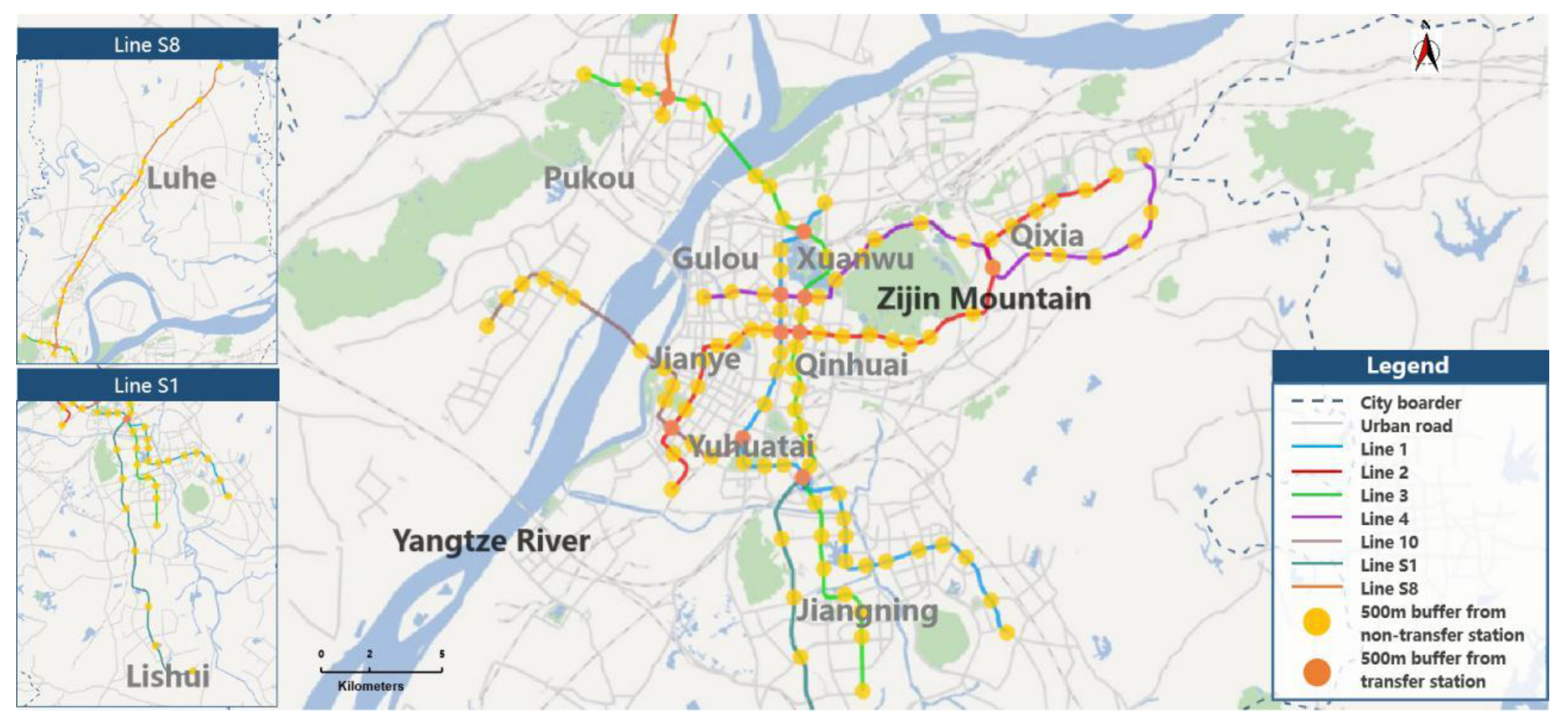
Nanjing, the capital city of Jiangsu province, is the second largest city in East China, after Shanghai. It has a prominent place in Chinese politics, culture, history, education, and commerce. As of 2016, Nanjing accommodated 10.23 million citizens within an area of 6600 km2. The Yangtze River, the longest river in China, flows through Nanjing. Historical relics, monuments, mountains, natural scenic lakes, the Olympic Sports Center, and much more are situated in this both ancient and modern city. Besides, the city also boasts an efficient metro system. With the successful operation of Metro Line 1, Nanjing metro service first started in 2005. By the end of May 2019, the total length of metro lines was 378 km, ranked fourth in China, and seventh in the world. By 2023, fifteen metro lines will be built in Nanjing, with a total length of 578 km [31]. The metro system carried a daily average of 2.7 million passengers in 2017 [2]. The system consists of seven metro lines, covering 118 non-transfer stations and 10 transfer stations, as shown in Figure 1. According to the administrative districts of Nanjing, urban, suburban, and exurban areas were then designated [32,33]. Gulou, Xuanwu, and Qinhuai districts were designated as urban areas. Jianye, Yuhuatai, Pukou, Jiangning, and west of Qixia were suburban areas. Luhe, Lishui, and east of Qixia were exurban areas.
3.2. Data Source
The AFC system records every ride of the metro passenger and provides a large quantity of detailed information concerning passenger ID, card type, payment, boarding and alighting stations, boarding and alighting time, and count of card usage. Three weeks of smart card data with over 20 million records, collected from 4 September 2017 to 24 September 2017, were used in this study. Smart card data are stored in the Oracle database and we could obtain a complete origin-designation (O-D) pair of each trip through data transformation. Passenger rides of each station were aggregated by station number and card swiping time.
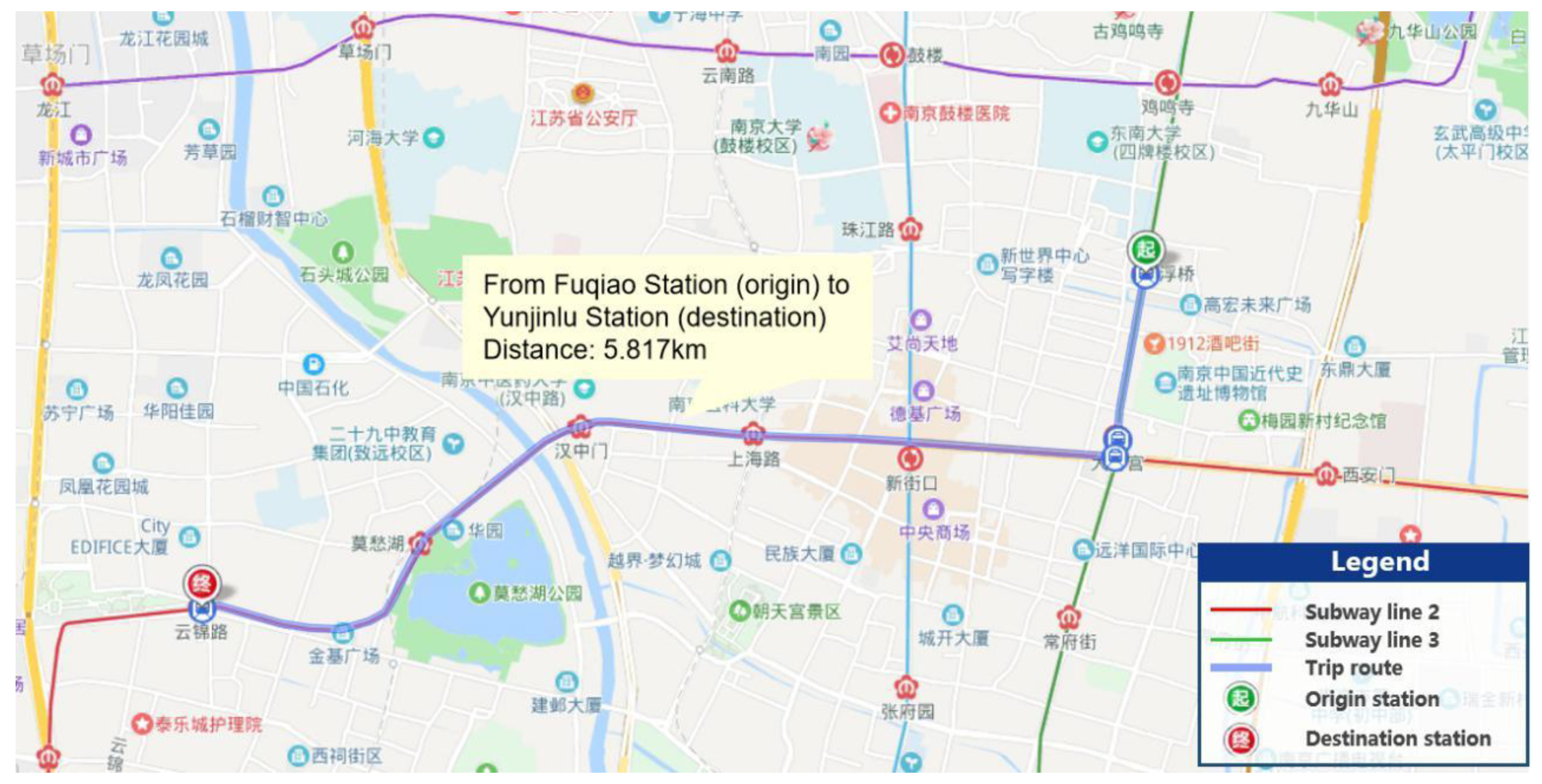
Baidu Map, one of the largest digital maps in China, could provide the route of each trip in its “route search” module based on the shortest path [34]. We may obtain the network distance of each trip by inputting the origin station and the destination station. Researchers have found this module is very reliable and intelligent in outputting up-to-date traffic information [35]. We thus designed a program to connect massive O-D pairs with the “route search” module and automatically calculated the network distance of each trip through the Baidu Map application programming interface (API). Figure 2 shows an example of a typical search. The network distance from Fuqiao Station (origin) in Subway Line 3 to Yunjinlu Station (destination) in Subway Line 2 is 5.817 km.
In recent years, point of interest (POI) data characterizing built environment have been used in some studies [36,37,38]. Generally, each POI record includes its own classification, name, address, coordinate, postcode, and administrative area [39]. Compared to traditional land use data, POI data have a greater flexibility in scale transportation. Massive POI data could fully reflect urban functions and greatly improve the explanatory power in modeling impacts of built environment on travel behaviors. Considering the pedestrian-friendly transit network in the planning of TOD, the radius of a pedestrian catchment area (PCA) was set to 500 m in many previous studies [37,40,41]. A PCA is generally defined as a geographical circle area where a great majority of pedestrians arrive on foot. It is determined by the maximum walking distance of passengers from/to the metro station [42,43]. Detailed information of POI data within a 500 m radius circle of each metro station was fetched through Gaode Map, a popular digital map service in China. A crawling program was written in Python to automatically gain POI data through the Gaode Map API. The date of crawling time was 12 September 2017, which remained consistent with the time of smart card data.
3.3. Variability of Station-Based Travel Distance
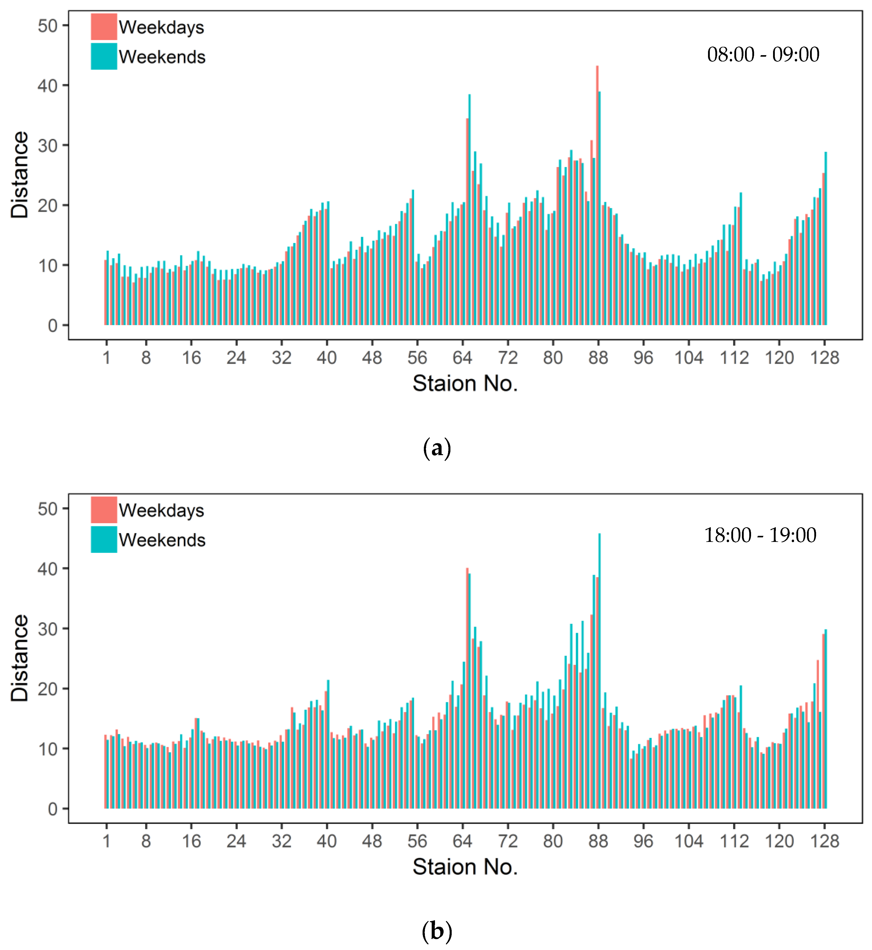
The variability of station-based travel distances is of fundamental importance to understand mobility patterns and the influences of the built environment. To identify the travel distance from place to place and from time to time, each trip record was projected into the spatial and temporal scale by aggregating station number and swiping time, respectively. Due to the space limitation, Figure 3 shows the bar graphs of travel distances from 08:00 to 09:00 and from 18:00 to 19:00 on weekdays and weekends. The x-axis is the station number and the y-axis is the average travel distance from the metro station in three weeks.
The overall tendencies of travel distances were similar on weekdays and weekends. Travel distances at some stations reached the highest during different periods. Spatial distributions of metro stations may be a major factor influencing the travel distances. In addition, there also existed moderate temporal variations. Travel distances on weekends were larger than those on weekdays at most stations. Free of work pressure, people were more willing to have long-distance travel with plenty of time on weekends, which was consistent with previous studies [15,44]. Meanwhile, as a station serves different groups of people throughout a day, differences in travel distance also exist during different periods. For example, boarding time for commuters is mainly distributed in the morning and afternoon. A station may serve a group of people from home to work in the morning and another group of people from work to home in the afternoon.
3.4. Dimensions of the Built Environment
Built environment data used in this study are derived from POIs. Based on our insights and determinants identified by previous studies, built environment variables were divided into two types to reflect the land use and transport facility. Land use is closely connected to travel behaviors, which has been proved by many studies [6,8,11,14]. According to the category of POI, this study extended the explanatory variables characterizing land use to a commuting group of variables and a non-commuting group, respectively. Within the commuting group, employment, residential buildings, education areas, and accommodation services were considered. In large cities, non-commuting activities also constitute an integral part of city life. Catering services, shopping services, leisure services, medical services, and scenic spots were thus included in this study. In addition, a dummy variable indicating whether a station is in the central business district (CBD) was also added to reflect the mixed land use.
Transport facility is also an important category that influences travel distance. Considering the multi-modal transferring completed by travelers, transport facilities relating to private car, bus, and public bicycle were all taken into account to explore the influences on metro travel distances. Thus, the number of public parking lots, public bicycle stations, bus stops, and bus lines within the catchment area of the station were calculated, respectively. Enhancing the level of connectivity is also significantly connected to metro use [43]. Urban roads and intersections were added to reflect the connectivity of metro stations. In addition, the characteristics of metro stations were also investigated by introducing the transfer dummy variable and the terminal dummy variable.
4. Methodology
4.1. Geographically and Temporally Weighted Regression
Station-based travel distances from the metro station vary over space and time. It is important to investigate spatial and temporal characteristics of travel behaviors in one unified model. The GTWR model is an expansion of the GWR model, which extends the traditional regression to address spatial and temporal heterogeneity simultaneously by estimating coefficients locally [45]. In this study, we applied the GTWR model to examine the spatio-temporal relationship between station-based travel distance and built environment. The fundamental formula of the GTWR model can be expressed as follows:
where yi is the average travel distance from the ith metro station. (ui, vi, ti) denotes the spatio-temporal coordinate of the ith station; βi0(ui, vi, ti) and βik(ui, vi, ti) are the intercept value and the local regression coefficients between travel distance and the kth built environment variable (explanatory variable), respectively; xik and εi are the value of the kth built environment variable and the random error, at station i, respectively.
Based on the assumption that closer observation to station i has a greater influence on the estimation of local coefficients, the estimated parameter βi(ui, vi, ti) is expressed as
where W(ui, vi, ti) = diag[wi1, …, wim] is the diagonal weighting matrix calibrated for station i. βi(ui, vi, ti) = (βi0, βi1, …, βim)T is the vector of m + 1 local regression coefficients for an intercept and m built environment variables. X = [x1T, …, xnT]T is the matrix of built environment variables. Y denotes the vector of travel distances. Decay-based Gaussian distance is employed as the kernel function to calculate the weighting matrix, which is defined as follows:
where wij is the calculated weighting parameter in the diagonal weighting matrix. Different from the GWR model, b and dij measure the spatial and temporal distance simultaneously. b is the bandwidth which determines the spatio-temporal range in the kernel function by producing a decay of influence with distance dij between stations i and j. dij is calculated as follows:
If the parameter λ equals zero, no spatial variation is estimated in the weighting function. This transforms the GTWR to the temporally weighted regression (TWR). On the other hand, if µ is set to zero, only spatial heterogeneity is analyzed in the model. This will lead to the traditional GWR model. Considering neither λ nor µ equals zero in most cases, this paper models the effect of built environment variables at both the spatial and temporal scales [45].
Let τ be the ratio parameter of µ/λ with λ ≠ 0. Then, the above equation can be transformed as follows:
To reduce computational complexity, λ can be set to one. τ is an essential parameter, which determines spatio-temporal effects of built environment on travel distances. wij depends on the bandwidth b that is an important parameter in calibrating the model. The minimum cross-validation (CV) criterion was employed to select an optimal value for the above parameter. The general mathematical form can be written as follows:
where is the predicted distance of yi referred as the function of bandwidth b in the GTWR model.
4.2. Spatial and Temporal Autocorrelation Test
In statistics, Moran’s I is used to detect the spatial autocorrelation of station-based travel distances and built environment variables among adjacent metro stations. For example, if stations are attracted by each other, it means nearby observations are spatially dependent. Moran’s I is defined as
where N is the number of metro stations. cij is an element of a spatial weighting matrix with zeros on the diagonal, which indicates the relationship of observations between two adjacent stations. zi and denote the variable of interest at station i, and the mean of z, respectively. The values of Moran’s I range from −1 to 1. If the observed value is significantly lower than −1/(N − 1), then it will represent spatial dispersion. When values are significantly larger than −1/(N − 1), it indicates a greater degree of spatial autocorrelation, suggesting a good GWR fit.
To detect the temporal autocorrelation of station-based travel distances throughout a day, this study applied Durbin-Watson (DW) test to measure the first-order temporal autocorrelation that is characterized by the similarity of a time series over successive time intervals [46,47]. The DW test, developed to test the null and alternative hypotheses, is shown as follows:
where the null hypothesis means that the errors of travel distances are not serially correlated. This will lead to no first-order autocorrelation. The alternative hypothesis of Ha means that the error item is correlated to the other error item in the previous period. The test statistic is formulated with the following equation:
where d is the DW statistic with a value from zero to four, and n is the number of observations. et and et−1 are the residuals from the ordinary least squares regression in the time period t and the time period t − 1, respectively. Each time period is set to an hour. When d-values equal to 2, there exists no autocorrelation in station-based travel distances. If d-values range from 0 to 2 (less than 2), positive temporal autocorrelation exists in the dataset. If d-values are between 2 (larger than 2) to 4, negative temporal autocorrelation is present in station-based travel distances.
4.3. Shannon Entropy Index
The Shannon entropy index (SEI), also known as Shannon’s diversity index, has been a popular quantitative index to study the level of heterogeneity in many fields [48]. The GTWR generally produced positive and negative local coefficients at different spatial and temporal scales after model estimations. Only using average values may not be enough to analyze spatial and temporal variations in built environment impacts, because positive and negative impacts may be compensated when coefficients were averaged. To overcome the problem, this paper thus used SEI to decompose the spatial and temporal heterogeneity of the coefficients estimated by GTWR models. This method could measure different types of built environment impacts and calculate how evenly built environment impacts are distributed among these types. The general equation of the SEI can be expressed as
where p1 is the proportion of coefficients of built environment variables above zero, and p2 is the proportion of coefficients below zero. The larger the h-value is, the greater the heterogeneity is. According to the theory of Limits, h approaches zero based on the above equation, if all coefficients are concentrated to one type of impacts and the other type is rare. As ln(0) is undefined, SEI is defined to be zero when p1 or p2 equals one.
5. Results
5.1. Model Calibrations
The GTWR models were calibrated based on the dependent and explanatory variables shown in Table 1. Before the weighted regression was developed, a stepwise regression was conducted based on the Akaike Information Criterion (AIC), in order to reduce multicollinearity and acquire a properly specified OLS model. Then, Moran’s I was calculated to identify spatial autocorrelation among metro stations. As shown in Table 1, coefficients of Moran’s I were significantly greater than expected values for all dependent variables and explanatory variables, with p-values being 0.000. This indicated that the values of dependent and explanatory variables were positively autocorrelated at the spatial scale. To further measure the temporal autocorrelation of traveling distance, a DW test was conducted to calculate the statistic parameters. d-values for travel distances on weekdays and weekends equaled 0.492 and 0.454, respectively. d-values were all between zero and two, with p-values being 0.000. Positive temporal autocorrelations existed for travel distances over successive time intervals. In addition, we conducted the Two-Sample t-test to examine the difference in station-based travel distances on weekdays and weekends. The result shows travel distances on weekdays are significantly different from ones on weekends at the 0.01 level.
5.2. Comparative Analysis of Different Models
When exploring the potential effects of built environment on metro travel distances, OLS, GWR, and GTWR were all developed to compare the performance of different models for each scenario. Parameters estimated in the OLS represent the general effects of the explanatory variables on travel distances. One direct model was developed for all metro stations. While using GWR and GTWR, different distance prediction models were developed simultaneously for each station. Meanwhile, GTWR considers the temporal variation throughout a day, compared to the GWR. Coefficients for each variable have spatially and temporally variations in GTWR.
The goodness-of-fit for each model are summarized in Table 2. It is observed that 37.8% of the variation in the travel distance values can be explained by the global OLS models in light of R2. Taking the weekday as an example, it should be noted that the proportion of explanation of variation in the travel distance increased from 0.378 in the global OLS model to 0.874 in GWR, and 0.894 in GTWR. By comparing the AICc in these models, the values decreased from 12867.41 in the global OLS model to 9637.35 in GWR, and 9399.63 in GTWR. Taking the residual sum of squares (RSS) into account, GTWR produced more accurate predictions. It is posited that GTWR captured the spatial and temporal heterogeneity of travel distances with better predictions. Simultaneously, comparative results also indicate that the improvement of GTWR over GWR was less than that of GWR over OLS in the model performance. A possible explanation for this finding is that the temporal heterogeneity of travel distance is less significant than spatial heterogeneity.
5.3. GTWR Estimates
The summaries of model estimates in the GTWR are shown in Table 3. Local parameters for travel distances of each scenario are described by four statistics that represent minimum values, mean values, maximum values and variables’ significance, respectively. Most variables were statistically significant at the 1% level, except for the three explanatory variables. It should be noted that the terminal dummy variable had no significant influence on travel distances for all scenarios. Travel distances from the terminal stations were not significantly different from ones at non-terminal stations. The positive/negative signs of the mean coefficients are similar for most variables on weekdays and weekends. The signs of the mean coefficients of shopping services, leisure services, public parking lots, bus stops, urban roads, and intersections were positive, which indicated that they were positively correlated to travel distances on weekdays and weekends. The signs of the mean coefficients of employment, scenic spots, and residential buildings were negative, which suggested that increasing their densities would decrease travel distance from the station. However, the absolute values of mean coefficients on weekends were greater than ones on weekdays, particularly for leisure services and scenic spots. Free of work pressure, people were more willing to undertake long distance travel for entertainment purposes on weekends [15,44]. Thus, the influences of these services on travel distances on weekends were far greater than weekdays.
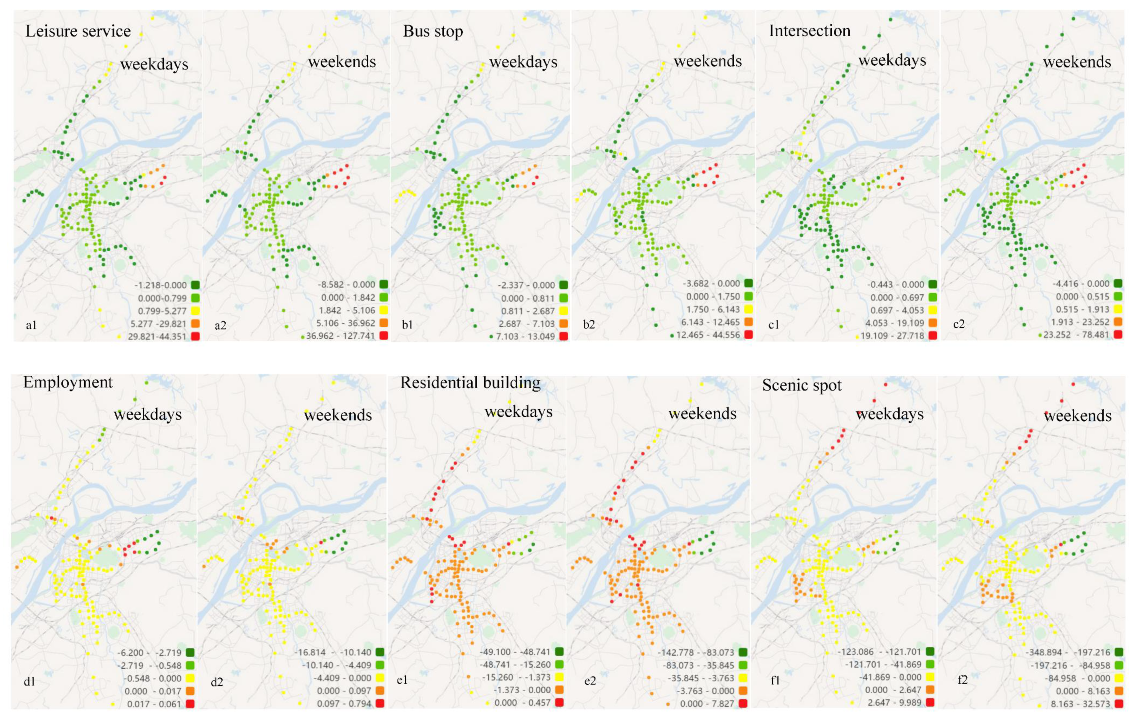
Spatial relationships between travel distances and built environment can be depicted for visual analysis through local coefficient estimates. Due to space limitation, leisure services, bus stops, intersections, employment, residential buildings, and scenic spots were visualized to reflect the effects of built environment, as shown in Figure 4. In this paper, the Jenks natural breaks classification method was used to determine the best arrangement of estimated coefficients into different classes. This method can minimize the average deviation of coefficients within classes and maximize the deviation between classes. Based on this method, the paper also manually sets zero as a breakpoint to differentiate the positive effects and negative effects. The general spatial variations of these six variables were similar between weekdays and weekends. It indicated that the positive and negative effects of built environment on travel distances were consistent in a week. Suburban and exurban areas imposed greater influences on travel distances, as depicted by the color of stations in Figure 4. Different from the mixed land use in the urban areas, suburban and exurban areas are usually characterized by single land use. Travel distances of people who live in remote areas are more sensitive than those living in the urban area.
The coefficients for leisure services were mostly positive in urban areas and exurban areas. Leisure services were densely distributed in urban areas, which attracted people to travel a long distance from other areas, especially on weekends. Due to the long distance from the urban areas, people in exurban areas might not travel a long way to urban areas while leisure services were rare. With cheaper land prices and less traffic congestion, suburban areas (e.g., Pukou) have ushered in a rapid development to reduce the pressure of urban areas and increase the city vitality in recent years. They usually have more attractions to exurban areas than urban areas in terms of geographical position. This also explains why the coefficients in urban areas were relatively small and the coefficients in some suburban areas were negative. Increasing leisure services in sub-centers would be an effective tool to decrease travel distance. The coefficients for bus stops were positive in most urban areas and exurban areas. Although urban areas had a high density of bus stops and population, metro travel distances were not necessarily short. People who had short-distance travel in the urban area could choose a public bicycle, bus or taxi. Considering travel time and costs, people who have long-distance travel might recognize metro as a better choice. As metro travels on segregated tracks, it has no competition for space with motor vehicles or buses. Efficient operations and low prices may attract long-distance travel. In most exurban areas, people often take the feeder bus to transfer to the metro, which takes passengers from an exurban area to an urban area. Thus, more bus stops contributed to longer travel distances. It should also be noted that the coefficients of some suburban and exurban areas were negative, probably because traffic conditions in these areas were better than urban areas. As a result, the bus then accounted for a large percent of long travel distance. The density of intersections was usually used to represent the street network connectivity [8]. If the number of intersections is larger within the PCA of a metro station, the catchment area then has greater connectivity. The coefficients of intersections were positive in Gulou, Xuanwu, Qinhuai, Qixia, and Pukou. It indicated that people tended to travel a longer distance in these districts, starting from stations with more connected street networks nearby. However, other districts (e.g., Jianye, Yuhuatai, Jiangning, and Lishui) exhibited the opposite results. A possible reason for this evidence is that people who travel in these three districts don’t need to cross the Yangtze River or Zijin Mountain. Other traffic modes (e.g., private car, bus, and taxi) may also be a good choice in terms of travel time if the connectivity of streets around the station is high.
The coefficients of the employment were mostly negative, which coincided with the previous study about VMT in North America [16]. It indicated that increasing job opportunities around residential buildings would reduce the travel distance between housing and work places. With higher coefficients, employment imposed greater influences on travel distances in the exurban areas. Few stations exhibited positive effects on travel distance, but, the corresponding coefficients were so small that they can be ignored. For residential buildings, the coefficients were also mostly negative in the city, except for some areas north of Pukou and Gulou. A possible explanation is that urban sprawl results in the dispersion of residential buildings [49]. Influenced by the problem of the separations between houses and work places, new areas with high residence densities are usually equipped with a low level of employment density. For stations with positive coefficients, they are not far away from urban areas and the land prices are relatively cheaper. High-density residential buildings are often distributed in these areas. With the limitations of land use, it is difficult to achieve an absolute balance between residence and employment. Some areas with high-density residence districts in the outer urban areas thus had long-distance travel characteristics. As the two most important commuting factors, there also existed some differences between employment and residence. The absolute coefficients of residential buildings were greater than those of employment, which indicated that the residence had more influence on travel distances than the employment. This is the image of other cities worldwide [7,50]. The coefficients of scenic spots were mostly negative, except for Jianye, Yuhuatai, and Luhe. The negative effects indicated that increasing scenic spots could also reduce travel distances to some degree. People usually go to scenic spots to alleviate work pressure and recharge the mind, body, and spirit. The influences of scenic spots on weekends were thus more significant, with the absolute values of coefficients being greater. Jianye, Yuhuatai, and Luhe districts all have positive effects on travel distances. A possible explanation is that many famous scenic spots in Nanjing are centered in these districts, such as Nanjing Olympic Center, Yuhuatai Scenic Park, Memorial Hall of the Victims in Nanjing, and Jinniu Lake. Different branches of these main scenic spots are distributed around those stations, which attract people from a long way away.
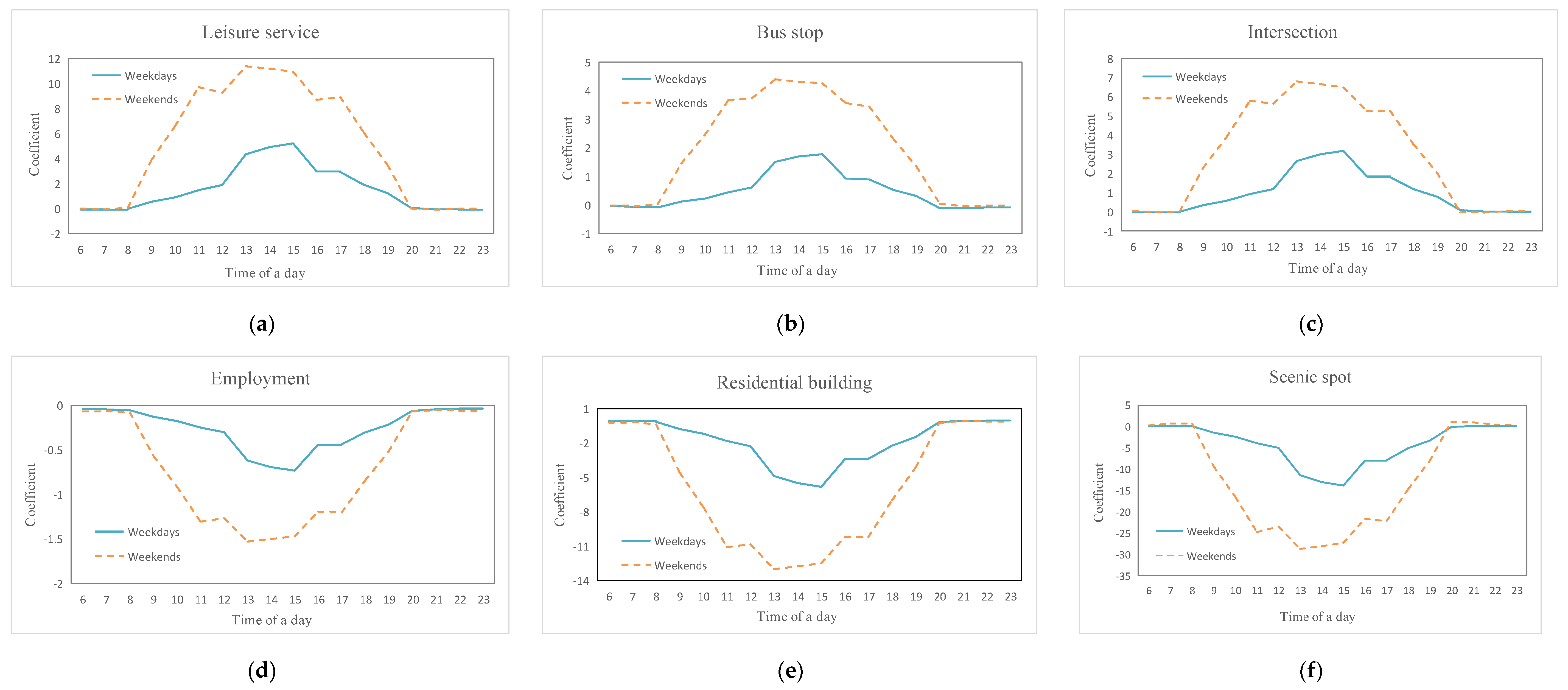
As an improvement to the GTWR model, a temporal dimension was incorporated into the traditional geographical dimension. Time series of coefficients can be obtained through data transformation. The temporal variations of the effects of built environment on travel distances are then depicted in Figure 5. Tendencies in the variations of leisure services, bus stops, and intersections were similar. Almost all coefficients for the three variations were positive in a week. Influenced by commuting characteristics, values of coefficients began to increase at 8:00. Peak values of travel distances appeared from 12:00 to 15:00 when built environment had the largest influence on travel distance. For the rest of the noon, the rate of change was relatively stable. After 15:00, values of coefficients started to decline until approaching zero at 20:00. During the afternoon, people are not willing to have long-distance travel, compared to the morning, probably because long-distance travel is time-consuming. The time they have left in the day may not be enough to satisfy their needs. Short-distance travel is a better choice for them. After 20:00, many retail services and other amenities are going to be closed. Thus, the effects of built environment approached to zero. In addition, the dashed lines in Figure 5 are all above solid lines for positive coefficients. It also indicates that built environment on weekends has greater influences than weekdays, which is consistent with the above findings. Different from the weekends, the values of coefficients of weekdays still increased at noon and began to decline after 15:00. The increasing demand for long-distance travel is more rigid on weekdays. In addition, employment, residential buildings, and scenic spots all have negative influences on travel distances in a week. Particularly, the absolute values of employment, residential buildings, and scenic spots have the same tendencies as the above variables. Given the similarities, the details will not be discussed.
5.4. Spatial and Temporal Heterogeneity
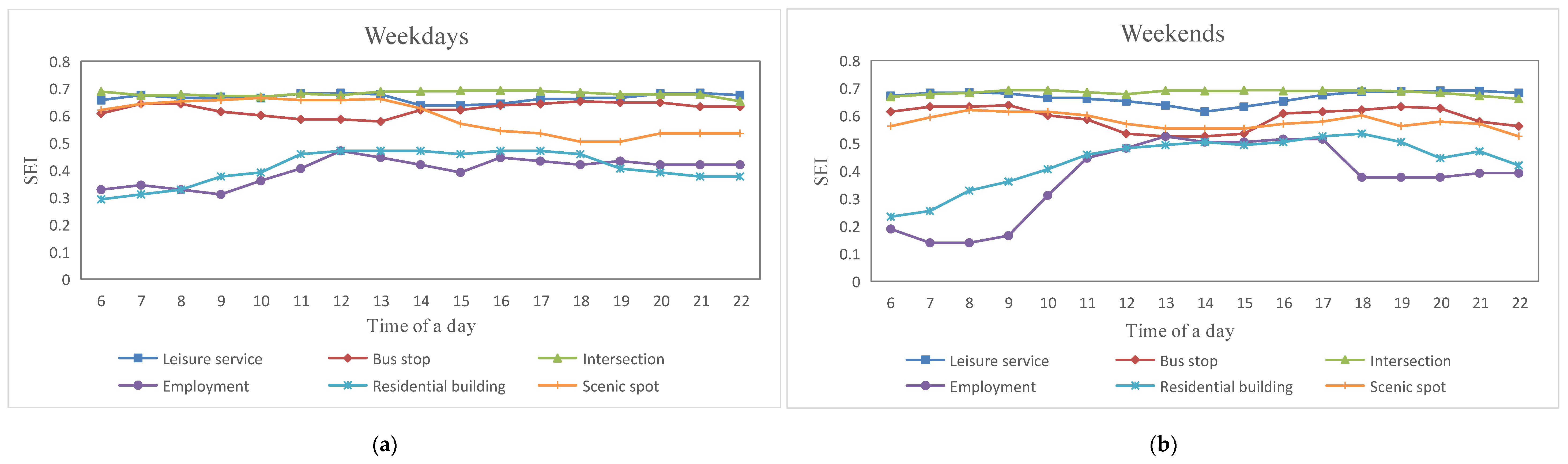
Average spatial and temporal features of coefficients were studied and discussed in previous sections. As positive and negative effects may be compensated by averaging, SEI was used in this paper to further quantify the degree of heterogeneity of built environment effects. The results of spatial and temporal heterogeneity are shown in Figure 6 and Figure 7, respectively. As to spatial heterogeneity at the temporal scale, leisure services and intersections both had significant spatial heterogeneity. The influence of intersections on travel distances remained stable without obvious fluctuations. The positive and negative effects of intersections around metro stations varied throughout the day. Different from other variables, connectivity represented by intersections generally did not vary with time. SEI of leisure services, bus stops, and scenic spots all declined at the beginning and rose up later. SEI of employment and residential buildings all exhibited an upward trend, then a downward trend. The findings reflect an obvious difference between non-commuting activities and commuting activities. The effects of non-commuting activity on travel distances are more heterogeneous than commuting activity at the spatial dimension. Meanwhile, the commuting activity on weekends also indicated a different fluctuation range, probably because many people do not have to work as usual on weekends. Others going to work may not necessarily obey the working time that is more flexibility on weekends.
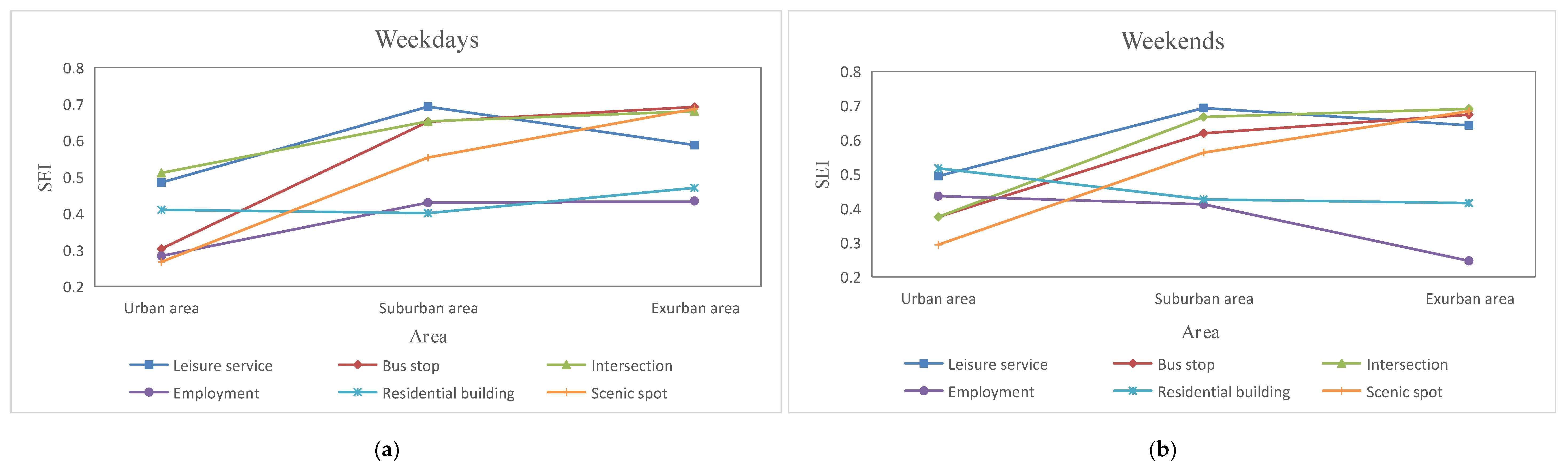
As for temporal heterogeneity at the spatial scale, the temporal heterogeneity of variables was projected into the urban, suburban, and exurban areas. SEIs of exurban areas were generally greater than other areas, followed by suburban areas. This means that higher temporal heterogeneity existed in exurban areas. Due to inconvenience in exurban areas, people’s demand for travel at different distances changed significantly throughout a day. As urban areas are equipped with relatively better facilities and services, people’s travel behaviors are relatively fixed throughout a day.
In addition, employment exhibited a different trend in a week. A possible explanation is the uneven distribution of industries in different areas. Some industries, such as financial, consulting and high-tech companies, still require people to work on weekends while others do not. Employment thus has a different pattern, compared to other variables.
6. Conclusions
This study offers additional analyses and implications for the connections between station-based travel distances and built environment by applying a framework that integrates GTWR and SEI. Unlike Western countries characterized by high car ownership, many cities in China are implementing TOD strategies. Understanding the influence of the built environment on metro travel behaviors is of vital importance to provide effective guidance for planning departments and transit agencies to alleviate traffic congestion and reduce transport emissions. Thus, the paper investigated the built environment and the mechanisms of the differences in station-based travel distances over space and time.
To the best of our knowledge, no previous study has analyzed travel distance based on smart card data. This paper used smart card data in modeling station-based travel distances in a broad view instead of survey data from previous studies. POI data characterizing built environment were also employed to reflect the land use and the transport facility, which shed light on the detailed information of urban land use and the understanding of transport facilities used by travelers. Results of the spatial and temporal autocorrelation tests indicate that it is necessary to take space and time into account in modeling travel distances. Space and time are two important dimensions for studying travel distances. To accommodate the spatial and temporal context where people make travel decisions, a GTWR model was applied to identify the spatial and temporal heterogeneity. The GTWR model showed a better performance of goodness-of-fit and achieved more accurate predictions, compared to the traditional OLS and GWR model.
According to the signs of mean coefficients, leisure services, shopping services, public parking lots, bus stops, urban roads, and intersections were positively correlated to travel distances. Employment, scenic spots, and residential buildings had negative effects on travel distance on weekdays and weekends. Meanwhile, the influences of these services on travel distances on weekends were far greater than weekdays. To visualize the variation patterns of the built environment effects on travel distances in GTWR models, average values of local coefficients were calculated based on space and time. People who live in exurban areas tended to travel in a long distance throughout the day. Built environment had more influences on metro travel distance at midday. Considering positive and negative effects may be compensated when coefficients were averaged, the paper further proposed SEI to quantify the degree of heterogeneity of built environment effects at the spatial and temporal scale. The effects of other factors, such as leisure services, on metro travel distances were more heterogeneous than residence and employment. Exurban and suburban areas with high heterogeneity can promote the mixed-use development to increase urban functionality and reduce travel distances and enhance community connections.
Living environment determines the spatial and temporal distribution of urban vitality as well as the dynamics of individual activities. On the other hand, the results in this study illustrate that the spatial and temporal variations of travel distances influenced by built environment also have significant implications in planning practices that can effectively improve land use and transport facilities at the local level. Reducing travel distances contributes to effectively cutting travel time, decreasing energy consumption, and playing a key role in the economy. Our findings from the perspective of travel behaviors can be used by planning departments to guide urban planning and neighborhood design. Based on the empirical study, transit agencies can optimize the metro operation to satisfy people’s need of traveling at different stations and during different periods. According to individual mobility and our findings, this study also helps residents choose the location of their home and enhance the accessibility to daily activities.
It should also be noted that the study only considered metro travel. Although the metro has accounted for the largest share of public transit ridership in Nanjing, bus and public bicycle modes should also be considered in future studies. As there is no need to swipe card to alight, the integrated circuit system in bus transit only records boarding time in most cities in China. Thus, it is difficult to acquire a complete and accurate O-D trip to calculate the travel distance. To solve this problem, future studies will focus on optimizing an algorithm of bus O-D pair inference and calculating multimodal transit travel distances based on smart card data.
Author Contributions
Conceptualization, E.C. and Z.Y.; Methodology, E.C.; Formal Analysis, E.C. and H.B.; Data Curation, E.C.; Writing-Original Draft Preparation, E.C.
Funding
This research was funded by the National Key R&D Program of China (No. 2018YFB1601000), the Scientific Research Foundation of Graduate School of Southeast University (No. YBPY1976), and the Jiangsu Transportation Science and Technology Project (No. 2019Y52).
Acknowledgments
We are grateful for the comments and suggestions from the editor and four anonymous reviewers who helped improve the paper.
Conflicts of Interest
The authors declare no conflict of interest.
References
- Beijing Municipal Transportation Commission. Transportation Statistics. Available online: http://www.jtw.beijing.gov.cn (accessed on 20 March 2019).
- Nanjing Transportation Bureau. Transportation Statistics. Available online: http://www.jtj.nanjing.gov.cn (accessed on 20 March 2019).
- Shanghai Municipal Transportation Commission. Transportation Statistics. Available online: http://www.jt.sh.cn/jtw/index.html (accessed on 20 March 2019).
- Cao, X. Examining the effect of the Hiawatha LRT on auto use in the Twin Cities. Transp. Policy 2018, 81, 284–292. [Google Scholar] [CrossRef]
- Huang, X.; Cao, X.; Yin, J.; Cao, X. Effects of metro transit on the ownership of mobility instruments in Xi’an, China. Transp. Res. Part D Transp. Environ. 2017, 52, 495–505. [Google Scholar] [CrossRef] [Green Version]
- Cervero, R.; Murakami, J. Effects of built environments on vehicle miles traveled: Evidence from 370 US urbanized areas. Environ. Plan. A 2010, 42, 400–418. [Google Scholar] [CrossRef]
- Choi, K. The influence of the built environment on household vehicle travel by the urban typology in Calgary, Canada. Cities 2018, 75, 101–110. [Google Scholar] [CrossRef]
- Diao, M.I.; Ferreira, J., Jr. Vehicle miles traveled and the built environment: Evidence from vehicle safety inspection data. Environ. Plan. A 2014, 46, 2991–3009. [Google Scholar] [CrossRef] [Green Version]
- Ding, C.; Mishra, S.; Lu, G.; Yang, J.; Liu, C. Influences of built environment characteristics and individual factors on commuting distance: A multilevel mixture hazard modeling approach. Transp. Res. Part D Transp. Environ. 2017, 51, 314–325. [Google Scholar] [CrossRef]
- Manaugh, K.; Miranda-Moreno, L.F.; El-Geneidy, A.M. The effect of neighbourhood characteristics, accessibility, home–work location, and demographics on commuting distances. Transportation 2010, 37, 627–646. [Google Scholar] [CrossRef]
- Singh, A.C.; Astroza, S.; Garikapati, V.M.; Pendyala, R.M.; Bhat, C.R.; Mokhtarian, P.L. Quantifying the relative contribution of factors to household vehicle miles of travel. Transp. Res. Part D Transp. Environ. 2018, 63, 23–36. [Google Scholar] [CrossRef]
- Ding, C.; Wang, D.; Liu, C.; Zhang, Y.; Yang, J. Exploring the influence of built environment on travel mode choice considering the mediating effects of car ownership and travel distance. Transp. Res. Part A Policy Pract. 2017, 100, 65–80. [Google Scholar] [CrossRef]
- Van Acker, V.; Witlox, F. Car ownership as a mediating variable in car travel behaviour research using a structural equation modelling approach to identify its dual relationship. J. Transp. Geogr. 2010, 18, 65–74. [Google Scholar] [CrossRef] [Green Version]
- Anastasopoulos, P.C.; Bin Islam, M.; Perperidou, D.; Karlaftis, M.G. Hazard-Based Analysis Travel Distance in Urban Environments: Longitudinal Data Approach. J. Urban Plan. Dev. 2012, 138, 53–61. [Google Scholar] [CrossRef]
- Holz-Rau, C.; Scheiner, J.; Sicks, K. Travel distances in daily travel and long-distance travel: What role is played by urban form? Environ. Plan. A 2014, 46, 488–507. [Google Scholar] [CrossRef]
- Hong, J.; Shen, Q.; Zhang, L. How do built-environment factors affect travel behavior? A spatial analysis at different geographic scales. Transportation 2014, 41, 419–440. [Google Scholar] [CrossRef]
- Wu, W.; Hong, J. Does public transit improvement affect commuting behavior in Beijing, China? A spatial multilevel approach. Transp. Res. Part D Transp. Environ. 2017, 52, 471–479. [Google Scholar] [CrossRef] [Green Version]
- Sun, B.; Ermagun, A.; Dan, B. Built environmental impacts on commuting mode choice and distance: Evidence from Shanghai. Transp. Res. Part D Transp. Environ. 2017, 52, 441–453. [Google Scholar] [CrossRef]
- Pelletier, M.P.; Trépanier, M.; Morency, C. Smart card data use in public transit: A literature review. Transp. Res. Part C Emerg. Technol. 2011, 19, 557–568. [Google Scholar] [CrossRef]
- Gong, Y.; Lin, Y.; Duan, Z. Exploring the spatiotemporal structure dynamic urban space using metro smart card records. Comput. Environ. Urban Syst. 2017, 64, 169–183. [Google Scholar] [CrossRef]
- Loo, B.P.; Chen, C.; Chan, E.T. Rail-based transit-oriented development: Lessons from New York City and Hong Kong. Landsc. Urban Plan. 2010, 97, 202–212. [Google Scholar] [CrossRef]
- Tao, S.; Rohde, D.; Corcoran, J. Examining the spatial–temporal dynamics of bus passenger travel behaviour using smart card data and the flow-comap. J. Transp. Geogr. 2014, 41, 21–36. [Google Scholar] [CrossRef]
- Zhong, C.; Manley, E.; Arisona, S.M.; Batty, M.; Schmitt, G. Measuring variability of mobility patterns from multiday smart-card data. J. Comput. Sci. 2015, 9, 125–130. [Google Scholar] [CrossRef]
- Helminen, V.; Ristimaki, M. Relationships between commuting distance, frequency and telework in Finland. J. Transp. Geogr. 2007, 15, 331–342. [Google Scholar] [CrossRef]
- Chen, F.; Wu, J.; Chen, X.; Wang, J. Vehicle kilometers traveled reduction impacts of transit-oriented development: Evidence from Shanghai city. Transp. Res. Part D Transp. Environ. 2017, 55, 227–245. [Google Scholar] [CrossRef]
- Wang, D.; Zhou, M. The built environment and travel behavior in urban China: A literature review. Transp. Res. Part D Transp. Environ. 2017, 52, 574–585. [Google Scholar] [CrossRef]
- Ding, C.; Liu, C.; Zhang, Y.; Yang, J.; Wang, Y. Investigating the impacts of built environment on vehicle miles traveled and energy consumption: Differences between commuting and non-commuting trips. Cities 2017, 68, 25–36. [Google Scholar] [CrossRef]
- Maat, K.; Timmermans, H.J.P. A causal model relating urban form with daily travel distance through activity/travel decisions. Transp. Plan. Technol. 2009, 32, 115–134. [Google Scholar] [CrossRef] [Green Version]
- Klinger, T.; Lanzendorf, M. Moving between mobility cultures: What affects the travel behavior of new residents? Transportation 2016, 43, 243–271. [Google Scholar] [CrossRef]
- Ma, X.; Liu, C.; Wen, H.; Wang, Y.; Wu, Y.J. Understanding commuting patterns using transit smart card data. J. Transp. Geogr. 2017, 58, 135–145. [Google Scholar] [CrossRef]
- General Office of the People’s Government of Nanjing. Nanjing “13th Five-Year” Public Transport Development Planning; General Office of the People’s Government of Nanjing: Nanjing, China, 2017.
- Yang, M.; Wu, J.; Rasouli, S.; Cirillo, C.; Li, D. Exploring the impact of residential relocation on modal shift in commute trips: Evidence from a quasi-longitudinal analysis. Transp. Policy 2017, 59, 142–152. [Google Scholar] [CrossRef]
- Yang, S.; Fan, Y.; Deng, W.; Cheng, L. Do built environment effects on travel behavior differ between household members? A case study of Nanjing, China. Transp. Policy. 2019, 81, 360–370. [Google Scholar] [CrossRef]
- Baidu Open Platform. Available online: http://lbsyun.baidu.com/ (accessed on 20 November 2017).
- Yang, Y.; Wang, C.; Liu, W.; Zhou, P. Understanding the determinants of travel mode choice of residents and its carbon mitigation potential. Energy Policy 2018, 115, 486–493. [Google Scholar] [CrossRef]
- Bao, J.; Xu, C.; Liu, P.; Wang, W. Exploring Bikesharing Travel Patterns and Trip Purposes Using Smart Card Data and Online Point of Interests. Netw. Spat. Econ. 2017, 17, 1231–1253. [Google Scholar] [CrossRef]
- Wang, Y.; Correia, G.H.d.A.; de Romph, E.; Timmermans, H.J.P. Using metro smart card data to model location choice of after-work activities: An application to Shanghai. J. Transp. Geogr. 2017, 63, 40–47. [Google Scholar] [CrossRef] [Green Version]
- Jappinen, S.; Toivonen, T.; Salonen, M. Modeling the potential effect of shared bicycles on public transport travel times in Greater Helsinki: An open data approach. Appl. Geogr. 2013, 43, 13–24. [Google Scholar] [CrossRef]
- Gaode Open Platform. Available online: http://lbs.amap.com (accessed on 12 September 2017).
- Lee, S.; Yi, C.; Hong, S.P. Urban structural hierarchy and the relationship between the ridership of the Seoul Metropolitan Subway and the land-use pattern of the station areas. Cities 2013, 35, 69–77. [Google Scholar] [CrossRef]
- Pan, H.; Li, J.; Shen, Q.; Shi, C. What determines rail transit passenger volume? Implications for transit oriented development planning. Transp. Res. Part D Transp. Environ. 2017, 57, 52–63. [Google Scholar] [CrossRef]
- Jun, M.; Choi, K.; Jeong, J.; Kwon, K.; Kim, H. Land use characteristics of subway catchment areas and their influence on subway ridership in Seoul. J. Transp. Geogr. 2015, 48, 30–40. [Google Scholar] [CrossRef]
- Zhao, J.; Deng, W.; Song, Y.; Zhu, Y. What influences Metro station ridership in China? Insights from Nanjing. Cities 2013, 35, 114–124. [Google Scholar] [CrossRef]
- Bekhor, S.; Cohen, Y.; Solomon, C. Evaluating long-distance travel patterns in Israel by tracking cellular phone positions. J. Adv. Transp. 2013, 47, 435–446. [Google Scholar] [CrossRef]
- Huang, B.; Wu, B.; Barry, M. Geographically and temporally weighted regression for modeling spatio-temporal variation in house prices. Int. J. Geogr. Inf. Sci. 2010, 24, 383–401. [Google Scholar] [CrossRef]
- Abdulhafedh, A. How to Detect and Remove Temporal Autocorrelation in Vehicular Crash Data. J. Transp. Technol. 2017, 7, 133–147. [Google Scholar] [CrossRef] [Green Version]
- Hilbe, J. Modeling Count Data; Cambridge University Press: Cambridge, UK, 2017. [Google Scholar]
- Palan, N. Measurement of Specialization the Choice of Indices; Research Centre International Economics (FIW): Vienna, Austria, 2010. [Google Scholar]
- Ta, N.; Chai, Y.; Zhang, Y.; Sun, D. Understanding job-housing relationship and commuting pattern in Chinese cities: Past, present and future. Transp. Res. Part D Transp. Environ. 2017, 52, 562–573. [Google Scholar] [CrossRef]
- Nasri, A.; Zhang, L. The analysis of transit-oriented development (TOD) in Washington, DC and Baltimore metropolitan areas. Transp. Policy 2014, 32, 172–179. [Google Scholar] [CrossRef]
Figure 1.
Nanjing metro network and study area.

Figure 2.
An example of route search in Baidu Map.

Figure 3.
Variability of travel distances at different times: (a) 08:00–09:00; (b) 18:00–19:00.

Figure 4.
Spatial distribution of the coefficients for built environment.

Figure 5.
Temporal distribution of the coefficients for built environment: (a) leisure service; (b) bus stop; (c) intersection; (d) employment; (e) residential building; (f) scenic spot.
Figure 5.
Temporal distribution of the coefficients for built environment: (a) leisure service; (b) bus stop; (c) intersection; (d) employment; (e) residential building; (f) scenic spot.

Figure 6.
Spatial heterogeneity at the temporal scale: (a) weekdays; (b) weekends.

Figure 7.
Temporal heterogeneity at the spatial scale: (a) weekdays; (b) weekends.


Table 1.
Descriptions of variables and descriptive statistics.
| Category | Variable | Description | Min | Max | Mean | S.D. | Moran’s I | Expected Value | p |
|---|---|---|---|---|---|---|---|---|---|
| Travel distance | DIS_WD | Travel distance from the metro station on weekdays (km) | 0 | 43.426 | 15.242 | 5.865 | 0.207 | −0.00046 | 0.000 |
| DIS_WK | Travel distance from the metro station on weekends (km) | 0 | 46.327 | 15.740 | 6.164 | 0.217 | −0.00046 | 0.000 | |
| Land use | Catering service | Number of Chinese, foreign restaurants, etc. | 0 | 840 | 121 | 167 | 0.150 | −0.00046 | 0.000 |
| Shopping service | Number of supermarkets, stores, appliance stores, etc. | 0 | 888 | 161 | 228 | 0.136 | −0.00046 | 0.000 | |
| Leisure service | Number of entertainment venues, gymnasiums, etc. | 0 | 186 | 17 | 27 | 0.160 | −0.00046 | 0.000 | |
| Medical service | Number of hospitals, clinics, pharmacies, etc. | 0 | 44 | 5 | 7 | 0.174 | −0.00046 | 0.000 | |
| Accommodation service | Number of hotels and guest houses | 0 | 187 | 19 | 31 | 0.109 | −0.00046 | 0.000 | |
| Employment | Number of government agencies, corporations, etc. | 0 | 974 | 110 | 182 | 0.213 | −0.00046 | 0.000 | |
| Scenic spot | Number of parks, plazas, tourist attractions, etc. | 0 | 20 | 3 | 6 | 0.259 | −0.00046 | 0.000 | |
| Residential building | Number of residential buildings | 0 | 22 | 6 | 6 | 0.156 | −0.00046 | 0.000 | |
| Education area | Number of schools, universities, etc. | 0 | 80 | 6 | 10 | 0.084 | −0.00046 | 0.000 | |
| CBD station | Station in the CBD (1 = yes, 0 = no) | 0 | 1 | N/A | N/A | 0.054 | −0.00046 | 0.000 | |
| Transport facility | Public parking lot | Number of parking lots | 0 | 120 | 27 | 24 | 0.235 | −0.00046 | 0.000 |
| Public bicycle station | Number of docked public bicycle stations | 0 | 10 | 2 | 2 | 0.104 | −0.00046 | 0.000 | |
| Bus stop | Number of bus stops | 0 | 10 | 4 | 2 | 0.070 | −0.00046 | 0.000 | |
| Bus line | Number of bus lines | 0 | 78 | 24 | 17 | 0.102 | −0.00046 | 0.000 | |
| Urban road | Number of roads | 0 | 20 | 5 | 5 | 0.222 | −0.00046 | 0.000 | |
| Urban intersection | Number of intersections | 0 | 57 | 13 | 12 | 0.194 | −0.00046 | 0.000 | |
| Transfer station | Transfer station (1 = yes, 0 = no) | 0 | 1 | N/A | N/A | -0.005 | −0.00046 | 0.000 | |
| Terminal station | Terminal station (1 = yes, 0 = no) | 0 | 1 | N/A | N/A | -0.004 | −0.00046 | 0.000 |
Table 2.
Comparison of goodness-of-fit for each scenario.
| Scenario | Goodness-of-Fit | OLS | GWR | GTWR |
|---|---|---|---|---|
| Weekdays | R2 | 0.378 | 0.874 | 0.894 |
| AICc | 12867.41 | 9637.35 | 9399.63 | |
| RSS | 46528.97 | 9430.47 | 7920.91 | |
| Weekends | R2 | 0.378 | 0.865 | 0.889 |
| AICc | 13084.41 | 9979.75 | 9747.19 | |
| RSS | 51361.15 | 11169.70 | 9202.34 |
Table 3.
Summaries of local parameters in the geographically and temporally weighted regression (GTWR) for each scenario.
Table 3.
Summaries of local parameters in the geographically and temporally weighted regression (GTWR) for each scenario.
| Variable | DIS_WD | DIS_WK | |||||||
|---|---|---|---|---|---|---|---|---|---|
| Min | Mean | Max | Significance | Min | Mean | Max | Significance | ||
| (Constant) | −30.996 | 14.898 | 32.955 | 0.000 ** | −56.485 | 14.015 | 44.886 | 0.000 ** | |
| Catering service | |||||||||
| Shopping service | −13.486 | 0.845 | 1.518 | 0.006 * | −18.612 | 1.488 | 4.836 | 0.004 * | |
| Leisure service | −5.922 | 1.654 | 161.564 | 0.005 * | −29.474 | 5.305 | 216.444 | 0.004 * | |
| Medical service | |||||||||
| Accommodation service | −6.241 | 0.069 | 10.200 | 0.005 * | |||||
| Employment | −21.640 | −0.271 | 0.296 | 0.002 * | −28.164 | −0.749 | 3.483 | 0.002 * | |
| Scenic spot | −425.749 | −4.398 | 12.171 | 0.005 * | −591.881 | −12.982 | 85.866 | 0.005 * | |
| Residential building | −174.579 | −1.957 | 6.043 | 0.003 * | −240.097 | −6.181 | 28.199 | 0.004 * | |
| Education area | −4.116 | −0.028 | 3.459 | 0.006 * | −10.053 | 0.073 | 8.132 | 0.004 * | |
| CBD station | −52.147 | 11.625 | 1486.557 | 0.142 | −296.008 | 35.604 | 2190.444 | 0.142 | |
| Public parking lot | −3.235 | 0.083 | 2.072 | 0.007 * | −2.968 | 0.022 | 1.877 | 0.007 * | |
| Public bicycle station | |||||||||
| Bus stop | −6.051 | 0.503 | 54.410 | 0.003 * | −10.739 | 2.055 | 76.644 | 0.004 * | |
| Bus line | |||||||||
| Urban road | −5.341 | 0.048 | 7.729 | 0.006 * | −8.312 | 0.689 | 17.946 | 0.008 * | |
| Urban intersection | −2.491 | 1.035 | 97.418 | 0.005 * | −16.863 | 3.164 | 132.275 | 0.003 * | |
| Transfer station | −17.295 | 0.898 | 240.860 | 0.130 | −113.909 | 5.704 | 284.608 | 0.131 | |
| Terminal station | −261.987 | −0.028 | 29.934 | 0.083 | −356.690 | −7.095 | 52.647 | 0.082 | |
| Goodness-of-fit | R2 | 0.894 | 0.889 | ||||||
| AICc | 9399.63 | 9747.19 | |||||||
Note: * refers to a value significant at the 0.01 level; ** refers to a value significant at the 0.001 level.
© 2019 by the authors. Licensee MDPI, Basel, Switzerland. This article is an open access article distributed under the terms and conditions of the Creative Commons Attribution (CC BY) license (http://creativecommons.org/licenses/by/4.0/).
Share and Cite
MDPI and ACS Style
Chen, E.; Ye, Z.; Bi, H. Incorporating Smart Card Data in Spatio-Temporal Analysis of Metro Travel Distances. Sustainability 2019, 11, 7069. https://0-doi-org.brum.beds.ac.uk/10.3390/su11247069
AMA Style
Chen E, Ye Z, Bi H. Incorporating Smart Card Data in Spatio-Temporal Analysis of Metro Travel Distances. Sustainability. 2019; 11(24):7069. https://0-doi-org.brum.beds.ac.uk/10.3390/su11247069
Chicago/Turabian StyleChen, Enhui, Zhirui Ye, and Hui Bi. 2019. "Incorporating Smart Card Data in Spatio-Temporal Analysis of Metro Travel Distances" Sustainability 11, no. 24: 7069. https://0-doi-org.brum.beds.ac.uk/10.3390/su11247069
Note that from the first issue of 2016, this journal uses article numbers instead of page numbers. See further details here.