Emissions and External Environmental Costs from the Perspective of Differing Travel Purposes


Institute of Transport Economics, University of Münster, Am Stadtgraben 9, 48143 Münster, Germany
*
Author to whom correspondence should be addressed.
Sustainability 2019, 11(24), 7233; https://0-doi-org.brum.beds.ac.uk/10.3390/su11247233
Submission received: 18 November 2019
/
Revised: 6 December 2019
/
Accepted: 12 December 2019
/
Published: 17 December 2019
(This article belongs to the Special Issue Sustainability Issues in Transport Pricing)
Abstract
:Comparisons of emissions and external environmental costs between transport modes usually focus on a distance-based approach. Emissions, and consequently the external costs of transport modes, are measured either per kilometer or passenger kilometer. For travel purposes such as holiday or leisure, however, this approach is not appropriate, as destinations are determined endogenously and thus distances vary across transport modes. In this study, we present a novel methodology to correctly and accurately measure leisure emissions and external costs. The new metric is called “full-price emissions”. Full-price emissions calculate the ratio of a transport mode’s emissions or external costs and its full price. The results show that the relative climate damage imposed by aircraft, calculated according to full-price emissions, is approximately four times larger than distance-based approaches reveal. We further observe that, in contrast to distance-based emission comparisons, environmental costs of petrol cars are lower than that of diesel cars. Additionally, full-price emissions display unintended substitution effects of environmental policies that can contribute to climate damage.
1. Introduction
Pollutant emissions and environmental effects attributed to climate change have received considerable attention in public debate. The global collective movement “Fridays for Future” brings millions of people around the world together to demonstrate against rising emissions, thus further promoting climate change. While improvements can be observed in several sectors, such as energy, emissions and environmental impacts caused by the transport sector continued to increase (especially CO2 emissions) over the last few decades [1]. In the European Union (EU), the transport sector accounts for around one quarter of total CO2 emissions, of which more than 55 % are from passenger transport [1,2,3].
The estimation and assessment of emissions is widely established and emission comparisons between transport modes regularly follow a distance-based approach. Emissions are measured either per kilometer or passenger kilometer (pkm), so that destinations are assumed to be exogenous. While this approach is appropriate for business trips or visiting family and friends, it may fail for other travel purposes like leisure or holiday, where destinations are determined endogenously. Consequently, distances can vary between transport modes and thus emissions can diverge even more. While research on distance-based transport emissions and environmental costs is extensive (see e.g., References [4,5,6,7]), there has been less research on whether these estimations are appropriate for different travel purposes.
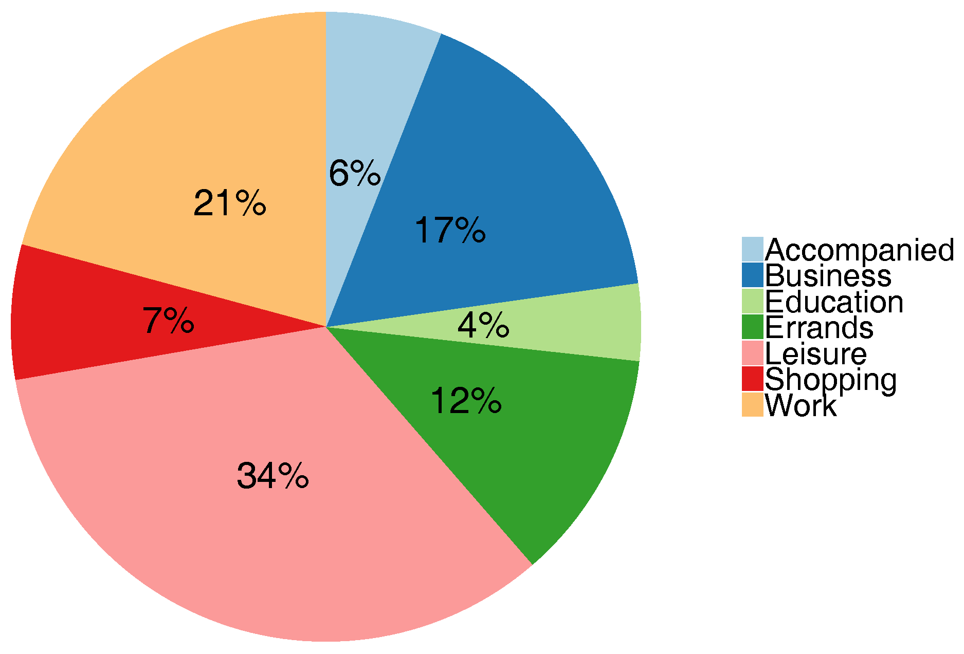
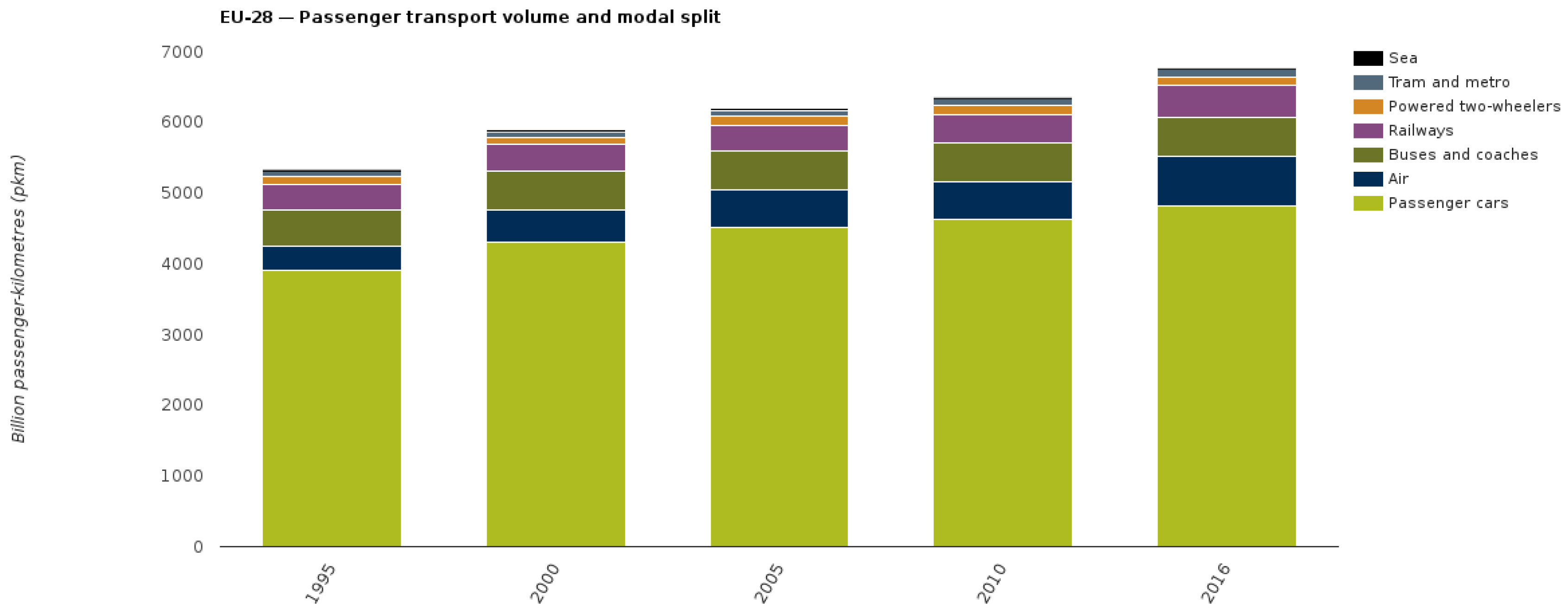
As leisure (and holiday, which is a subset of leisure trips) accounts for a large part of total passenger kilometers (e.g., 34% in Germany, see Figure 1), the estimation of emissions related to these travel purposes is important in order to reveal the climate impact that different journeys can impose. As mentioned, the characteristic feature of holiday or leisure trips is that destinations are often determined endogenously. However, this depends on the preferences of a consumer. If a consumer wants to visit a specific city, for example Berlin, then implicitly the destination is no longer endogenous. There is partial endogeneity if a consumer wants a beach holiday but does not know the exact destination. Our assumption of (full) endogeneity, however, refers to cases where a consumer decides to spend some time away from home in order to relax or have a good time. This applies especially to leisure activities or short holidays, since the main determinants are the monetary as well as the time budget (see for example González-Savignat [8] for factors influencing leisure travellers). For such travel purposes, consumers can choose between various alternatives, for example, a holiday at the Baltic Sea (by car) or on Mallorca (by aircraft). Thus, the distance/destination choice is actually part of the choice set, in addition to the choice of the transport mode. Therefore, distance-based emission comparisons cannot correctly represent the environmental impacts of such travel purposes. Consequently, the aim of this paper is to fill this research gap and develop an approach to estimating emissions and (external) environmental costs for travel purposes with endogenously determined destinations. Accordingly, this research project provides an innovative methodology for estimating transport emissions related to travel purposes that represent a significant proportion of total passenger kilometers. We refer to this approach as full-price emissions. The approach builds on our prior research [9] but is extended to further emission categories and external costs. As indicated by its name, full-price emissions treat the full price of transport, which is defined as the sum of ticket price and time cost (i.e., the monetary value or the “price” of travel time, see for example References [10,11]), as the decision variable. For example, a consumer going on vacation decides to spend an extended weekend and determines a budget of 600 Euros (EUR). Implicitly, part of this budget of money and time is reserved for transport. Given a fixed full-price budget for transport, the climate impact of each transport mode is different. Building the ratio of emissions and full-price budget yields the metric for full-price emissions, which is designed to calculate the relative climate impact of each transport mode, related to travel purposes like leisure or holiday [9].
While in principle, we confirm the results of prior research in this field, we also add new insights by showing that the negative climate impact of aviation is even more pronounced when destinations are endogenous, compared to when they are exogenous. That is, for a given full-price budget, aviation emissions are 10 to 12 (moderate scenario) up to 30 (extreme scenario) times higher than for coaches (most environmentally friendly transport mode). If destinations are assumed to be exogenous, this factor reduces to 8. Additionally, we show that environmental costs of diesel cars are higher compared to petrol cars (assuming average size fleets), whereas traditionally diesel cars are assumed to be more environmentally friendly. The new full-price emissions approach enables us to display possible environmental effects of environmental tax or pricing policies. More specifically, full-price emissions demonstrate that environmental policies focusing on one specific transport mode can cause an increase in environmental damages related to leisure/holiday trips. In this way, full-price emissions contribute to evaluating the effects of different policy measures.
The remainder of this paper is structured as follows. Section 2 contains an overview of the literature on (distance-based) emissions, as well as on the external environmental costs of transport. The data and methodology for calculating full-price emissions are outlined in Section 3. In Section 4, the analysis and results are presented. Section 5 discusses the results and Section 6 draws some conclusions.
2. Literature Review
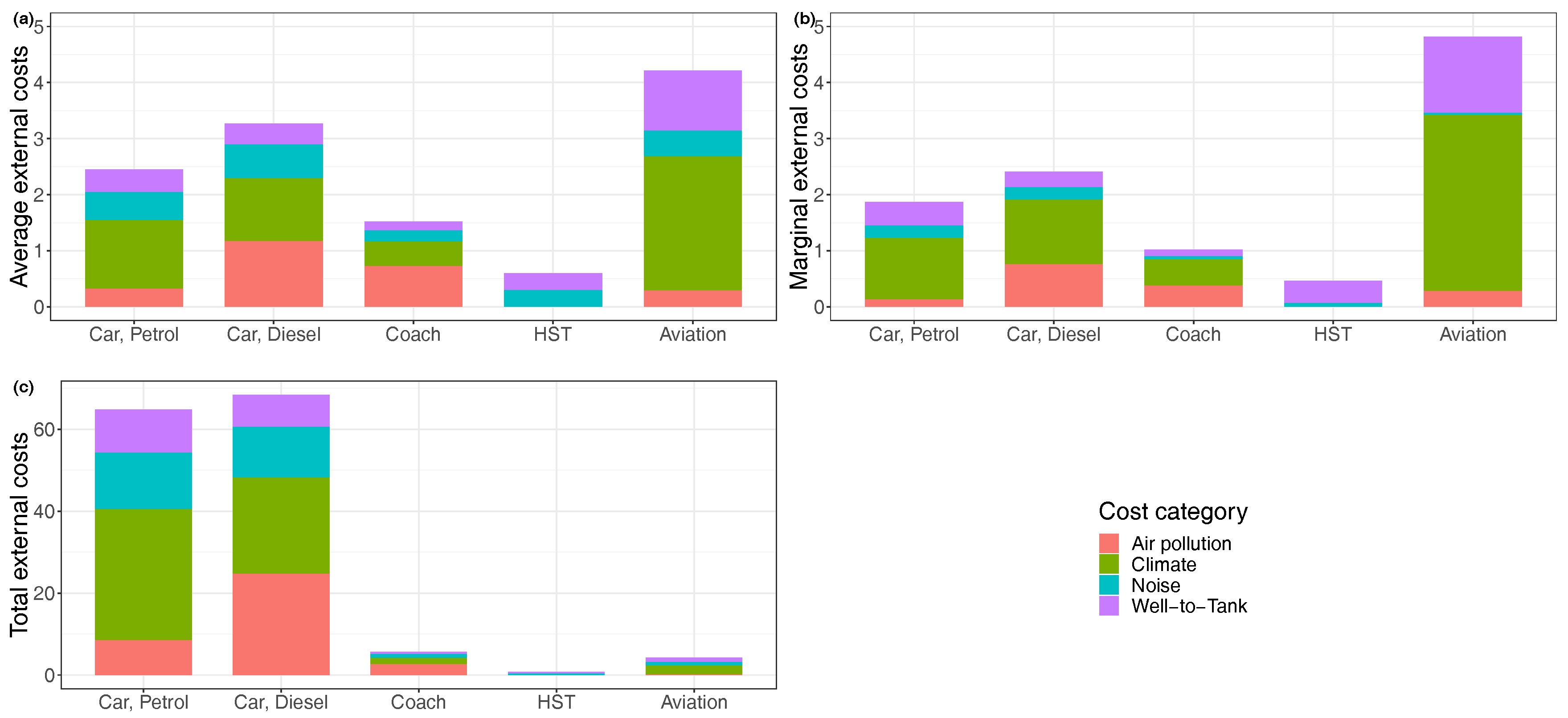
At a European level, the most relevant study dealing with external costs of transport, and thus with external environmental costs, is the Handbook on the External Costs of Transport by CE Delft [4], which was updated in early 2019. In this study, the total, average and marginal external costs of different transport modes and vehicle types are calculated for 2016. External environmental costs include noise costs, air pollution costs, climate change costs and costs of well-to-tank emissions. To determine emissions and external costs, the study relies mainly on data from Eurostat and the emissions model COPERT. Additional data is derived from port authorities and the Handbook of Road Transport Emission Factors (HBEFA 3.3). The study finds that road transport causes by far the highest external environmental costs and cars account for a large part of total external environmental costs (see Figure 2c). When looking at average external costs, that is, the ratio of total external costs and (passenger) transport performance, the results change (see Figure 2a). This difference can be explained partly by the high share of trips made by car (modal split > 70%, see Figure A1). Nevertheless, the study concludes that there are more environmentally friendly means of transport than travelling by car. Especially, high-speed train (HST) or coach travel only cause moderate average external costs compared to other transport modes. The figures for aviation are an average of short, medium and long-haul flights. Thus, average external costs are likely to be underestimated; especially if the figures are used for a comparison between transport modes. Since competition between the transport modes takes place primarily on short-haul journeys (see References [8,13]), the difference in average external environmental costs will be larger than depicted in Figure 2a. This can be explained by the larger share of the landing and take-off cycle as well as the smaller aircraft size (less efficient) and its lower occupancy rate.
Moreover, the study calculates marginal external costs. “Marginal external costs are the additional external costs occurring due to an additional transport activity” [4]. They are relevant for assessing the economically efficient internalisation of external costs for different transport modes (referred to as 1st best or marginal cost pricing). Cost factors are presented for different Euronorm categories of each vehicle type (see Figure 2b). The study finds that marginal external environmental costs through air pollution and climate change do not depend on the traffic density, as the amount of air pollutant emissions does not depend on whether a car enters a dense or a thin traffic flow (assuming that other factors, for example speed and location, remain the same). However, marginal noise costs depend to a high degree on local factors, for example population density, existing noise levels and time of day. Thus, they are subject to higher variation [4].
Besides the European studies, there are several national ones estimating passenger transport emissions or environmental costs. In general, the results do not differ excessively from the abovementioned. For example, the German Environment Agency conducted a study calculating marginal environmental costs in Germany. They use data from the TREMOD model (Transport Emission Model) as well as emission factors from HBEFA 3.3 to determine the vehicle emissions [5]. The study considers air pollutants, greenhouse gases, noise, energy supply as well as other infrastructure/pre-process-related environmental costs (e.g., land consumption and fragmentation). Cost factors are, similar to the abovementioned study, reported for different Euronorm categories of each vehicle type. Differences in the results are due to the use of a higher carbon dioxide cost rate of €180/t CO2 (compared to €100/t CO2 in Reference [4]) or from other ways of calculating the emissions (e.g., different emission models).
The German Environment Agency also provides estimates of emission factors (see Table 1) [6]. These express kilometer-related emissions, assuming an average occupation of each transport mode (i.e., grams per pkm (g/pkm)). They represent the traditional approach to determining emissions, since distances/destinations are assumed to remain exogenous. Usually, this approach is also used for emission-calculating programmes, which calculate emissions for specific distances or routes by using emission factors. Often, they focus only on emissions of CO2, as other pollutants make up a smaller share of total transport emissions. For example, the “Verkehrsclub Deutschland” (German Transport Club) estimates the emissions of CO2 of different transport modes on the Berlin-Frankfurt link [7]. Both emission comparisons identify coaches as the most environmentally friendly transport mode, followed by HST, whereas aviation exhibits the highest average emission factors.
3. Data and Methodology
While the abovementioned studies focus on the estimation of emissions and environmental damages, we now want to analyse emissions and the resulting external costs for travel purposes characterized by endogenous destinations. Therefore, we basically rely on two data components. First, we have to determine emission and external cost factors, which we use to estimate emissions and the external environmental costs of different transport modes. Second, we have to calculate full prices, which capture monetary costs of the journey as well as time-related (opportunity) costs. These two parts are described in Section 3.1 and Section 3.2. Section 3.3 deals with the new methodological approach to determining full-price emissions.
3.1. Emission and External Cost Factors
To estimate emissions and external costs, we build on the data described in Section 2, that is, we use the external cost factors from CE Delft [4] to calculate environmental impacts. The approach used in their study is widely established and therefore can be regarded as valid. The study is also continuously improved methodologically, as it is updated regularly. However, one drawback is that the database (level of transport-mode-specific emissions) is not freely accessible. As a consequence, it is not possible to determine the emission factors used in Reference [4] from the external cost estimates and damage-cost factors. Thus, we estimate emissions on the basis of average emission factors from the German Environment Agency (see Table 1) [6]. Additionally, we use greenhouse gas emission factors as reported by an emissions calculator [14], which uses data based on the same emission model (TREMOD) as the data from the German Environment Agency. This enables us to provide estimations for coaches offering scheduled transport services, as well as for both diesel and petrol cars. As can be seen in Table 1, petrol cars produce equivalent greenhouse gas emissions to diesel cars, despite their higher average fuel consumption. This reveals that indirect emissions from fuel production (well-to-tank emissions) are higher for diesel cars, which is to a large extent a result of the transformation of diesel fuel [16]. Hydrocarbon (HC) and particulate matter (PM) emission factors are considered to be identical across vehicle types (petrol and diesel cars), either because PM emissions mainly result from tyre, brake and road abrasion or because emissions of HC are relatively low and do not vary significantly between petrol and diesel cars. As the emission factors of the German Environment Agency are not differentiated between petrol and diesel cars, we rely on nitrogen oxide (NOX) emission factors from the Austrian Environment Agency [17]. These are comparable to other studies which calculate NOX emission factors [18,19]. Since emission factors of the Austrian Environment Agency are given in grams per vehicle kilometer, we divide them by the load factor to obtain emission factors in g/pkm. The factors reflect that diesel cars emit significantly higher NOX than petrol cars, due to higher combustion temperatures, which are necessary for the fuel efficiency of diesel engines. Due to missing data, we estimate the emissions of carbon monoxide (CO) on the basis of the average value for passenger cars published by the German Environment Agency. Accordingly, we assume that the emissions of diesel and petrol cars are evenly/uniformely distributed around the mean value and take the share of passenger kilometers made by diesel and petrol cars into account [20]. This assumption seems reasonable, as the limit values for CO emissions (which are regulated by the european authorities) of petrol cars are twice as high as those of diesel cars (1 g/km for petrol cars, 0.5 g/km for diesel cars [21]).
In determining the external costs we rely on marginal external cost factors, as one aim of this paper is to stress the problems resulting from (additional) transport activities and the potential environmental effects of different policy measures. As applied in Section 2, we focus on external costs from air pollution, greenhouse gases and energy or fuel supply (well-to-tank emissions). We ignore noise costs, as they are subject to higher uncertainties than the other pollutants due to a larger dependency on local factors.
The assessment of air pollution costs follows a damage-cost approach. Thus, damages caused by air pollutant externalities are valued by applying emission factors to cost factors per pollutant. Environmental impacts through air pollution are estimated by an impact-pathway approach. This approach calculates environmental impacts through modeling the atmospheric dispersion of emissions as well as their concentration [4]. The resulting cost figures are presented in Table 2, where the figures within each regional area are averaged over different road types. Although some information might get lost, we can reasonably argue that this approach is valid, as the figures within each regional area do not differ excessively. Additionally, in this section we focus on representative vehicles of each transport mode rather than on the average fleet.
Climate-change costs are another source of environmental cost. These costs place a value on emissions of greenhouse gases like CO2, N2O and CH4. The respective emissions are converted into CO2-equivalent emissions by using Global Warming Potentials (GWP), such that total greenhouse gas emissions can be determined. External costs due to climate change are then estimated by using an avoidance-cost approach. This approach focuses on the cost of achieving a specified policy target (e.g., EU CO2 reduction targets). Therefore, an avoidance-cost function is determined, which calculates the cost of a reduction of one additional tonne of CO2. Ultimately, the minimum of the cost function is estimated (so as to meet the policy target) [4]. The results for marginal climate change costs are presented in Table 3.
Environmental costs also include those of well-to-tank emissions, that is the external costs resulting from energy production. These cover both the environmental impacts of electricity production as well as of fossil fuel production. The production process involves the extraction, processing, transport and transmission of electricity and fossil fuels. Especially the costs of electricity production are country-specific, as they depend on the electricity generation mix in each country. Thus, the EU28-average values presented in Table 4 should not be considered as representative for specific countries. However, as the focus of this study is on the methodological approach for determining emissions for various travel purposes, average values will not bias the results significantly.
3.2. Full Prices
For leisure and holiday trips, there are various determinants of the decision to travel to a certain destination. Among others, these include the budget, type of trip (city trip, beach holiday, etc.) and/or the availability of transport mode alternatives [22]. In general, a consumer is not constrained in his travel decision. If he chooses to determine one factor of those mentioned above, the decision problem reduces. For example, if the consumer decides on a beach holiday, destinations are constrained. On the other hand, if the consumer determines a vacation budget, he will be able to choose the transport mode as well as the destination. This implies that both decisions become endogenous. Following the line of reasoning of Adler et al. [13], Behrens/Pels [23], Eisenkopf et al. [22] and González-Savignat [8], the price is the main determinant of leisure or holiday trips. Concerning travel time as a determinant of leisure or holiday trips, the studies yield diverging results. While Behrens/Pels [23] find no signifcant effect of travel time for leisure travellers, González-Savignat [8] shows that leisure travellers are sensitive to travel time, although not to the same degree as business travellers. We stick to the result of González-Savignat and argue that travel time is a relevant determinant of leisure or holiday trips, because consumers usually want to spend as much time as possible at the destination and thus derive disutility from travel time. Therefore, we can reasonably assume that consumers determine an amount of money and time for an activity or vacation for leisure or holiday trips. Note that this way of thinking for leisure and holiday trips is markedly different to business trips or visiting family and friends, where destinations are exogenous and thus partly also the transport mode (as some destinations can be reached only with certain transport modes due to infrastructure restrictions). Note further that the endogeneity of destination and transport-mode choice for leisure and holiday trips implies the following: First, consumers can decide among a choice set consisting of different transport-mode-destination combinations. Second, to restrict the choice set of a (representative) consumer, we need to determine a decision variable. As argued above, this is the full price of a journey, since a consumer usually determines the duration and budget of a journey before making decisions. The full price is the product of the distance and the full-price factor , where the latter is the sum of ticket-price factor (travel cost per pkm) and time-cost factor (per pkm).
Time costs are a passenger’s cost of ”suffering” from travel time (opportunity costs). The time-cost factor is the product of a transport mode’s average speed (h/km) and distance-based travel-time cost factors (€ per person and hour, see Appendix B, Table A1).
Average speeds of different transport modes are obtained from TREMOD (see Appendix B, Table A2 for input values) [24]. However, there are no data for average speeds of trains and (short-haul) aviation. Thus, we rely on estimates based on our own calculations for several relations and on prior research [25]. (We collected a sample of approximately 20 German inter-urban rail connections. Travel times were obtained from the travel information of Deutsche Bahn. Distances were calculated by manually mapping the routes using OpenStreetMap within the open source software Qgis. For aviation, we applied a comparable approach by selecting approximately 20 routes originating from different German airports. We then calculated the ratio of aerial distance and travel time.) Furthermore, as there were no major developments or technical improvements over the last decade, average speeds will not have significantly changed. Besides, the calculated values seem to be in line with observations in prior literature [26]. Following González-Savignat [8] and Adler et al. [13], we consider additional time costs at airports as occurring due to check-in and check-out processes. We therefore apply a value of 1.5 h as the overall pre- and post-process operations for each flight. In order to assess the opportunity costs, we weight this additional time by the value of time estimates for non-business trips (€ 15.54) which is used for Cost-Benefit Analysis of transport infrastructure investments [27].
Ticket-price factors of public transport (including aviation and coaches) are approximated by using yields (i.e., revenues per pkm). These enable us to calculate full-price emissions independent of destinations. They also reflect that, on average, travel costs increase with distance, that is, the further away a destination, the more expensive the journey. Yields were collected from (annual) financial reports of transport companies and crosschecked with several studies on fare factors [28,29,30].
For passenger cars, an equivalent approach is to calculate distance-based travel costs, that is, we approximate the marginal costs of car usage. These include fuel cost, kilometer-related depreciation and maintenance and repair costs [9]. The calculation of car costs is based on three car segments (small, compact, midsize) and two fuel types (petrol, diesel). The chosen car segments account for the highest share in Germany’s car stock in 2018. We assign a representative car model to each combination of car segment and fuel type, based on the best selling models in Germany in 2018. (The following representative car models for petrol are chosen: Volkswagen Polo VI 1.0 MPI (small), Volkswagen Golf VII 1.0 TSI (compact), BMW 320i (midsize); and for diesel: Volkswagen Polo VI 1.6 TDI (small), Volkswagen Golf VII 1.6 TDI (compact), BMW 318d (midsize).) We obtain maintenance and repair costs from the car cost calculator of the German Automobile Club (ADAC) [31]. As indicated by Reference [32], we assume an average useful life of 12 years for privately used vehicles and that half of the depreciation is attributable to mileage. To calculate the depreciation per vehicle kilometer, we use vehicle prices derived from the car cost calculator and an average annual mileage of 15,000 km, which is approximately equal to the value reported in the German mobility survey Mobilität in Deutschland [12]. Fuel costs are determined using operating costs as reported in the car cost calculator. We then determine the marginal costs of car usage by weighting the model-specific costs by the proportion of the models in the total vehicle fleet. Finally, we divide the resulting value by the load factor to obtain a figure in €-Cent/pkm.
3.3. Methodological Approach for Full-Price Emissions
The basic input factors necessary for estimating full-price emissions were presented above. These are used to calculate a full price according to Formula (1). As we specified the full price as the exogenous decision variable for leisure and holiday trips, destinations and consequently transport modes remain endogenous. Our approach to assessing full-price emissions now proceeds as follows: A (representative) consumer determines a full-price budget for transport. This budget allows the consumer to choose between various combinations of distance and transport mode. Due to the different levels of full-price factors (see Appendix B, Table A2) a consumer can reach different distances with each transport mode. Imagine that a consumer wants to spend €100 on transport to go on holiday. Now, both lower ticket prices as well as lower travel time costs (due to higher average speeds) promote higher distances for aviation, compared to other modes of transport. We operationalize this approach by rearranging Equation (1) to obtain maximum mode-specific distances that can be reached with a given full-price budget :
We thereby assume that a consumer invests the whole amount of €100 in transport and chooses for each transport mode those destinations that are furthest away. Consumers might determine a budget for the entire holiday and thus react not only to changes in travel costs but also to changes in hotel prices. Since considering the budget for the entire holiday would cause an additional variability which is not related to the transport modes, full-price emissions ignore this fact. Additionally, we rely on this assumption, as we wish to emphasize the possible effects of deviations from the 1st-best pricing and especially low air fares.
Finally, we determine full-price emissions by calculating the ratio of the product of maximum mode-specific distances and average emission factors and the fixed full-price budget.
4. Analysis and Results
In this section, we present the results of our calculations for two different travel purposes, business trips (exogenous destination) as well as leisure/holiday trips (endogenous destination). We proceed in two steps. First, we estimate emissions per person from the average emission factors in Table 1. The second step is to weight the resulting emissions by the damage-cost factors of the respective pollutants (see Appendix B, Table A3) to obtain (external) environmental costs. Additionally, we then compare the results with values that are computed directly from (marginal) external cost factors as reported in the EU study [4] (see Section 3.1). Finally, we compare the new metric for full-price emissions with the traditional distance-based emission metric.
4.1. Emissions
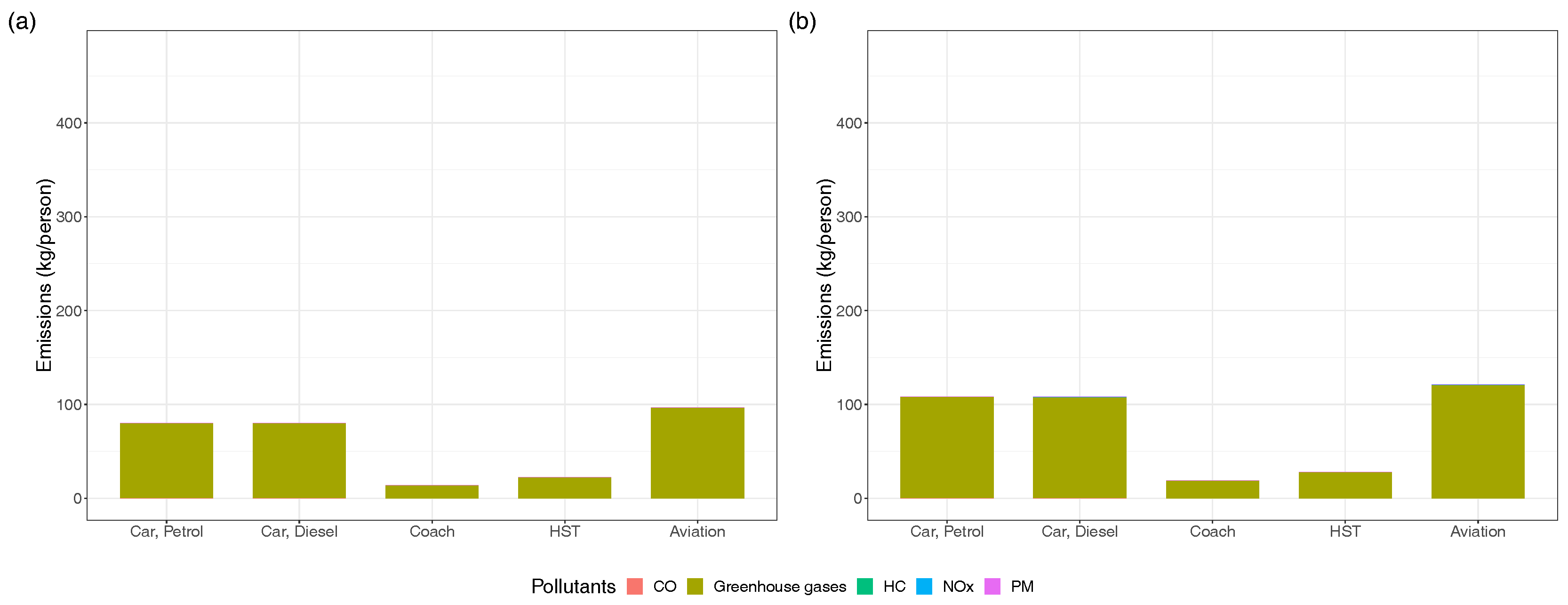
We compute emissions per person for both travel purposes by calculating the product of emission factor and distance travelled. For holiday trips, the results of aviation are further differentiated between two different carriers, low-cost carriers (LCCs) and ultra-low cost carriers (ULCCs). If we look at the European airport market, this might correspond to Eurowings and Ryanair, respectively. Thus, we use the average fares of these carriers to calculate the corresponding full prices. The aim is to compare emissions between two carriers that offer low-cost flights (to a different extent) and especially to emphasize the effects that low air fares impose on emissions. For each travel purpose, we investigate the emissions on two routes (distance-based approach) or two scenarios (full-price emissions). We start by displaying the emissions per person that represent the reference scenario or the ‘standard case’, as applied in the literature. Transport emissions are compared on two different routes (see Figure 3). This applies to the case of business trips where destinations are determined exogenously.
Therefore, we select two routes which represent a typical business trip. The first route extends from Cologne/Bonn to Berlin, which is a typical trip for members of federal ministries who commute between Bonn and Berlin (as some ministries are located either in both cities or in one city). The results of the corresponding calculations are reported in Figure 3a. For all transport modes, emissions of greenhouse gases are the main source of pollution. Other pollutant emissions (CO, HC, NOX, PM) account for a negligible share of total emissions. Coaches exhibit the lowest emissions per person, whereas cars and aviation produce approximately 6 times more. Especially the small difference between cars and aviation is striking. Possible explanations are on the one hand lower load factors of cars (resulting in higher emission factors) and on the other hand larger distances, as the cars actual travel distance is larger than the aerial distance. The results can be confirmed when looking at the second route from Hamburg to Munich (see Figure 3b).
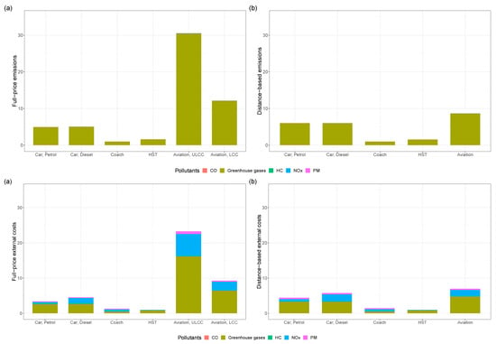
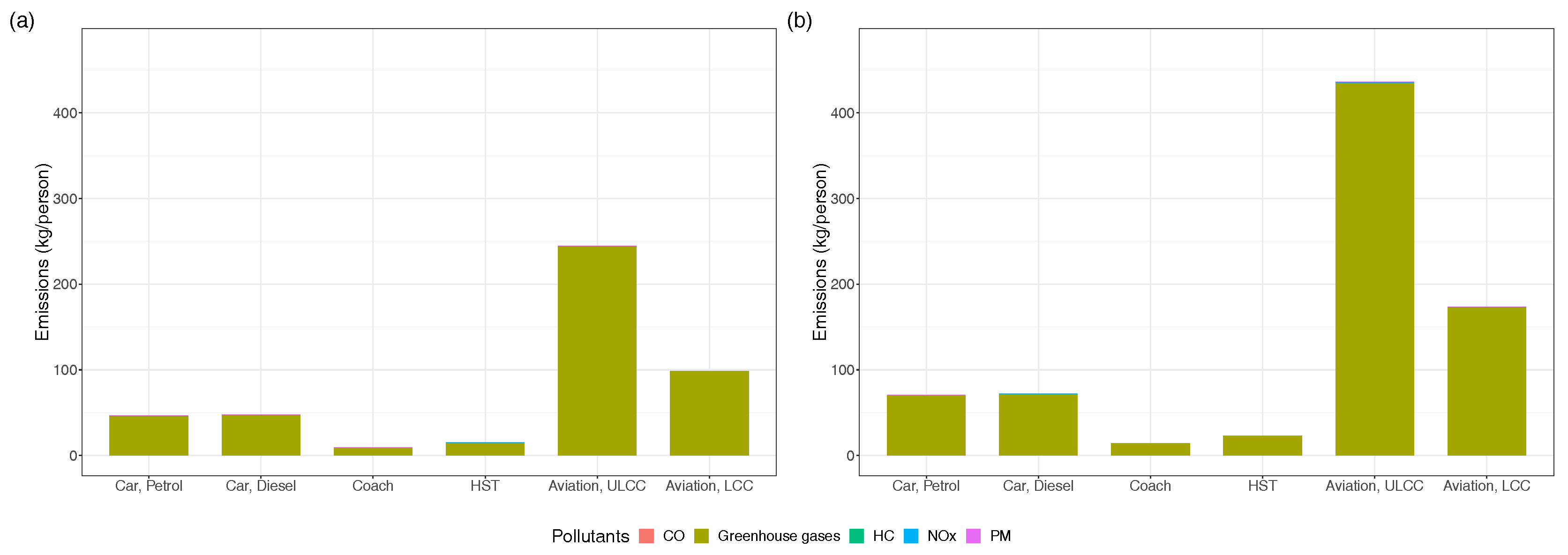
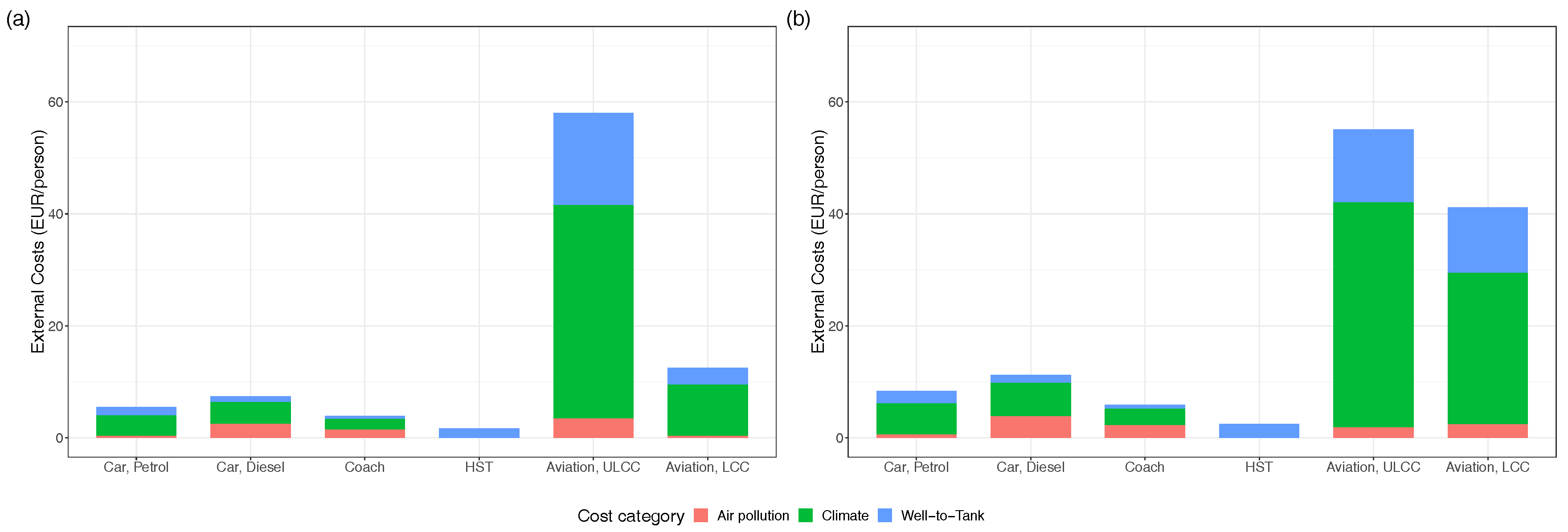
Figure 4 depicts the results of the full-price approach, assuming endogenous destinations and average load factors. Because one might reasonably argue that holiday trips are made with the family, so that using average load factors (especially for cars) is not suitable, we present an analysis of a “family scenario” at the end of this subsection. However, we first stick to the approach of using average load factors in order to obtain an unbiased comparison between distance-based and full-price emissions. Furthermore, several national travel surveys show that the difference in average occupancy rates between various travel purposes is not very significant [33,34,35]. We find that, given a fixed budget, emissions per person are much higher for aviation and lower for other modes of transport compared to Figure 3 (this depends however, on the determined full-price budget). In Figure 4a, for example, we calculate emissions per person for a full-price budget of = €100 per person. On this basis, we proceed as explained in Section 3.2 and Section 3.3.
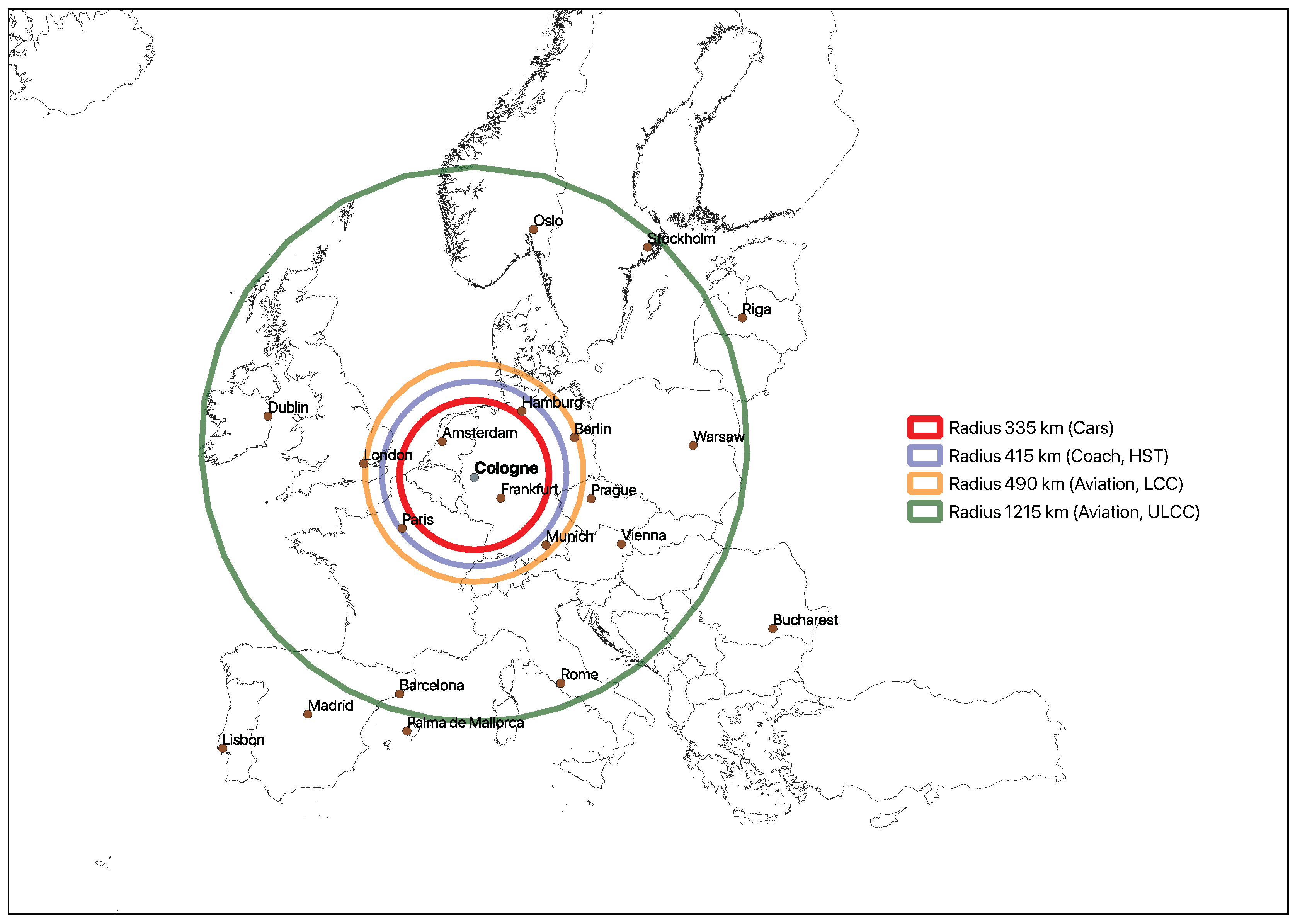
That is, we firstly determine maximum transport-mode-specific distances. For the purpose of illustration, we display these distances in Figure 5, where we summarize the results for cars as well as coaches and HST in one category each, as their maximum distances differ only by 10 to 15 km. For all radii, Cologne was chosen as the point of departure. The outer edge of the circles around the starting point then display the maximum transport-mode-specific distances for the given full-price budget. We find that a consumer can travel the largest distance by aviation (∼1215 km ⇔ Mallorca), whereas all other transport modes yield similar distances (∼330–420 km ⇔ North Sea/Baltic Sea). Consequently, this contributes to a higher climate disadvantage of aviation.
It is also useful to investigate the composition of the full-price budgets. While for cars and HST, the full prices are split approximately equally between travel costs and time costs, the full price of coaches reveal an imbalance, with a stronger weight on time costs (70 to 30 %). This is a consequence of the low average speed of coaches. Considering aviation, we see a difference between the two carriers. While full prices for ULCCs reveal a stronger weight on time costs than on travel costs (60 to 40 %), there is a stronger weight on travel costs for LCCs (63 to 37 %). As average speeds are assumed to be identical, this result is mainly driven by higher travel-cost factors of LCCs, compared to ULCCs. These lead to a significant difference in emissions between the two types of carriers, which indicates the severely negative environmental effects of low air fares.
In general, the findings confirm the intuition that lower travel costs and higher average speeds work to increase distances and therefore emissions. Especially average speeds have a considerable influence on the results, as they implicitly determine the distances. Since aircraft exhibit significantly higher average speeds than other modes of transport, they can travel larger distances in less time. And, as emissions accumulate with distance, aircraft produce significantly higher emissions for equivalent budgets. Other determinants that affect the results are related to the emission factors. These are average emissions and load factors, which determine the level of the emission factors. Consequently, lower average emissions as well as higher load factors decrease average emission factors and thus improve the environmental performance.
As mentioned above, various factors can impact on environmental performance. Among others, these include average load factors, which might also be linked to the travel purpose. In particular, it can be expected that average load factors for holiday trips are higher than for business trips (this holds true especially for cars) [33,34,35]. Consequently, this has an impact on the results. To account for this issue, we investigate a scenario for families. The average load factors directly affect the ticket-price factor and the average emission factor . However, the effect is restricted to cars, since travelling with a family, using a coach, HST or aviation, has no significant influence on the average price per pkm. For the same reason, average emission factors of these transport modes are not, or are only minimally affected. Furthermore, an additional family member might simply take up a seat that would otherwise be used by another passenger, thus not affecting the average occupation. There are, however, differences if we look at cars. The ticket-price factors which are approximated by the marginal cost of car usage can now be split among more passengers, thus reducing the average price per pkm. This implies that, given a fixed full-price budget, people can travel larger distances by car. Additionally, a higher load factor reduces the average emission factor accordingly. The effects work in opposite directions. While larger distances increase emissions per person, lower average emission factors reduce them. We find that the positive effect of lower average emission factors is stronger than the negative effect of larger distances. This follows from the composition of the full price. Since the full price is the sum of ticket and time costs and occupation only affects the ticket-price factor, the total effect on the full-price factor is rather small. By contrast, a higher load factor unfolds its full impact on the average emission factors. Consequently, this yields lower emissions per person for cars, compared to the average-occupancy scenario displayed in Figure 4. Considering a family of four, the reduction amounts to approximately 50% (see Appendix D, Figure A2 for the results). As expected, we observe a positive effect of average occupation on emissions per person, that is, the higher the occupation of a car, the lower the emissions per person, given a fixed full-price budget per person.
4.2. (External) Environmental Costs
In addition to comparing the emissions related to both travel purposes, we also investigate (external) environmental costs of those travel purposes. Thereby, we use two approaches. First, we use the above calculated emissions, which we value with damage-cost factors to obtain environmental costs. Second, we calculate external environmental costs directly from external cost factors as given in Reference [4]. By doing so, we are able to verify the calculations within this section.
4.2.1. External Costs through Weighting Emissions with Damage-Cost Factors
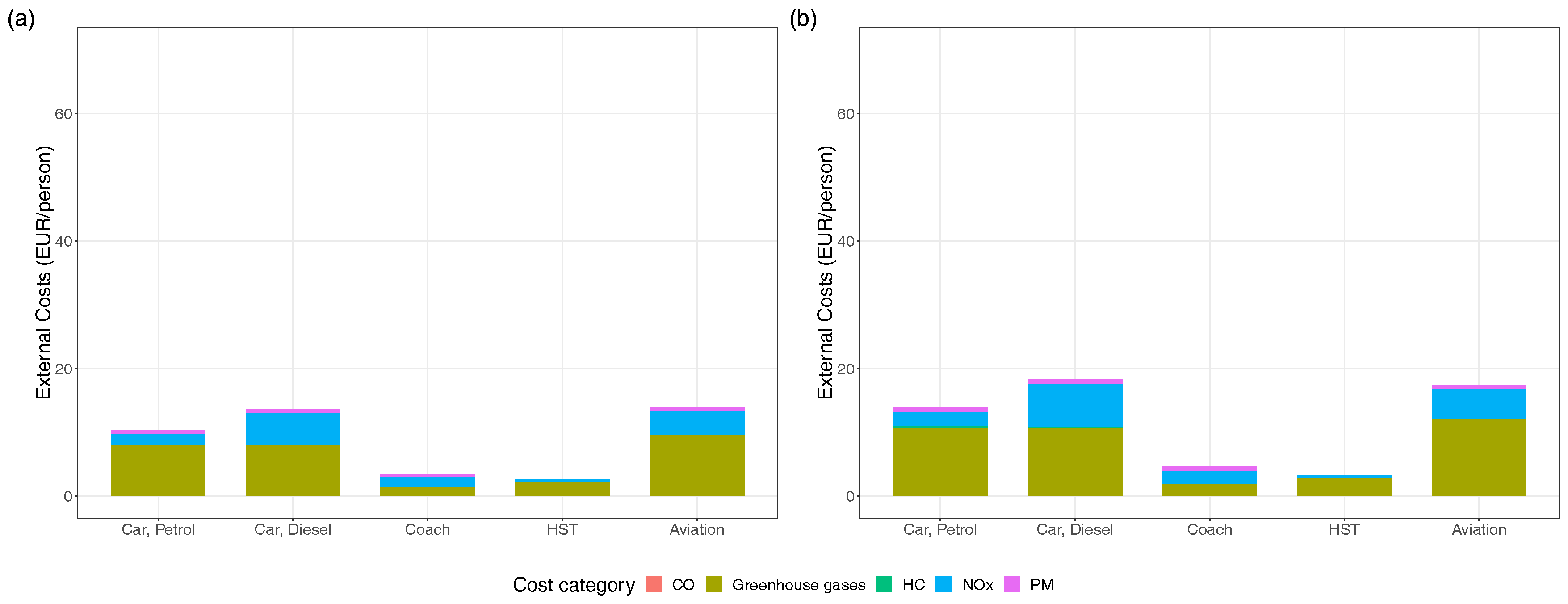
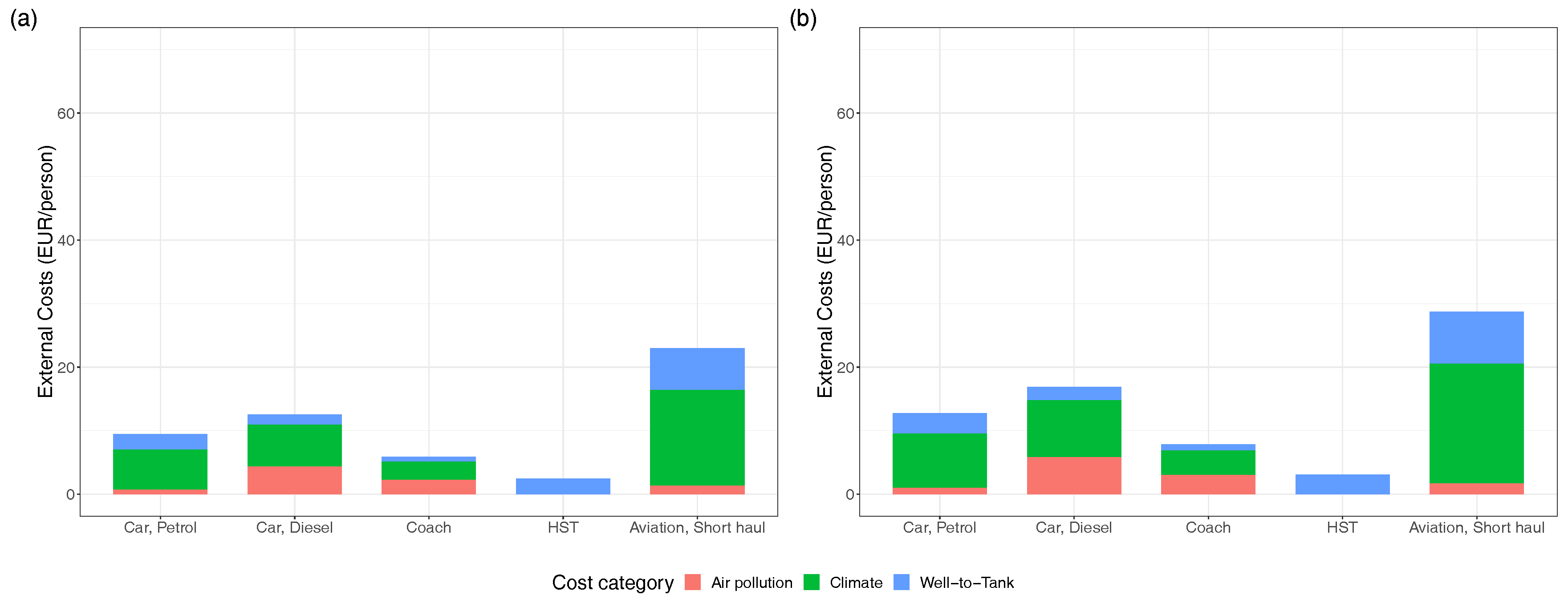
The first approach to determining environmental costs is to use damage-cost factors (see Appendix B, Table A3), which are multiplied by the emissions per person calculated in the previous section. The results for business trips are shown in Figure 6. Greenhouse gases again account for the highest share of environmental costs produced by different transport modes. Nevertheless, it becomes obvious that the share of environmental costs due to other air pollutants, especially NOX, significantly increase. The reason is the different levels of damage-cost factors. A possible explanation for these different damage-cost factors is that the pollutants affect environment, health and other damages to a varying degree. All in all, this leads to changes in the ranking of environmental performance. Diesel cars and coaches are found to cause more environmental costs than petrol cars and HST, whereas the analysis of emissions in the previous section revealed the opposite. The higher environmental costs of these vehicles stem from the fact that diesel engines (coaches are usually operated with diesel fuel) emit higher levels of NOX, which are valued at a significantly higher damage-cost factor than greenhouse gases or CO (see Appendix B, Table A3). This has the consequence that the environmental cost performance of diesel cars is nearly as poor as aviation in this comparison. Their performance is 5 to 6 times poorer than that of the HST.
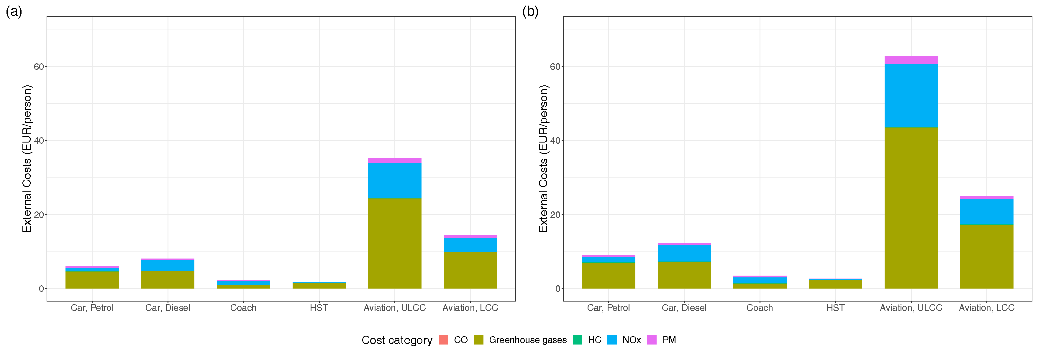
Figure 7 displays the results for holiday trips. Again, environmental costs due to greenhouse gases represent the highest share of total environmental costs. In this comparison, the environmental costs of aviation are highest for the same reasons mentioned in Section 4.1. First, higher average speeds and second, lower ticket prices promote longer trips resulting in higher emissions and consequently, higher environmental costs per person. Furthermore, it can be observed that within each emission category (except CO), aviation causes the highest environmental costs per person. Again, the difference between the two air carriers is remarkable and thus emphasizes the negative effect of low air fares. Considering the scenario of a family, the results of Section 4.1 apply to the comparison of environmental costs as well, that is, the higher the occupation of a car, the lower the environmental costs per person.
4.2.2. External Costs through Marginal External Cost Factors from CE Delft [4]
The second approach to calculating external environmental costs uses the marginal external cost factors as reported in CE Delft (for selected values, see Section 3.1). We weight the factors by the share of EURO classes within each vehicle category, so as to obtain weighted marginal external cost factors (see Appendix C, Table A6). Cost factors are given in €-Cent/pkm. These are multiplied by the distance, so as to obtain external environmental costs per person.
The results for business trips are shown in Figure 8. It is evident that external costs are slightly higher than the above results. Nevertheless, the ranking of transport modes does not change, as aviation still causes the highest, and HST the lowest, external costs per person.
In Figure 9, the results for holiday trips are displayed. In general, the results presented in Figure 7 can be confirmed. However, the following differences should be noted. First, environmental costs for a full-price budget of €160 concerning an ultra-low cost flight are lower compared to the lower budget of €100. This is due to medium-haul cost factors, which have to be applied as the distance increases (i.e., if the distance > 1500 km). These are significantly lower, as emissions are passed on to more passengers. Second, in this particular case, this leads to a higher environmental cost disadvantage of aviation for lower-budget travellers (6 to 30 for = €100, 14 to 19 for = €160).
4.3. Comparison between Distance-Based Emissions and Full-Price Emissions
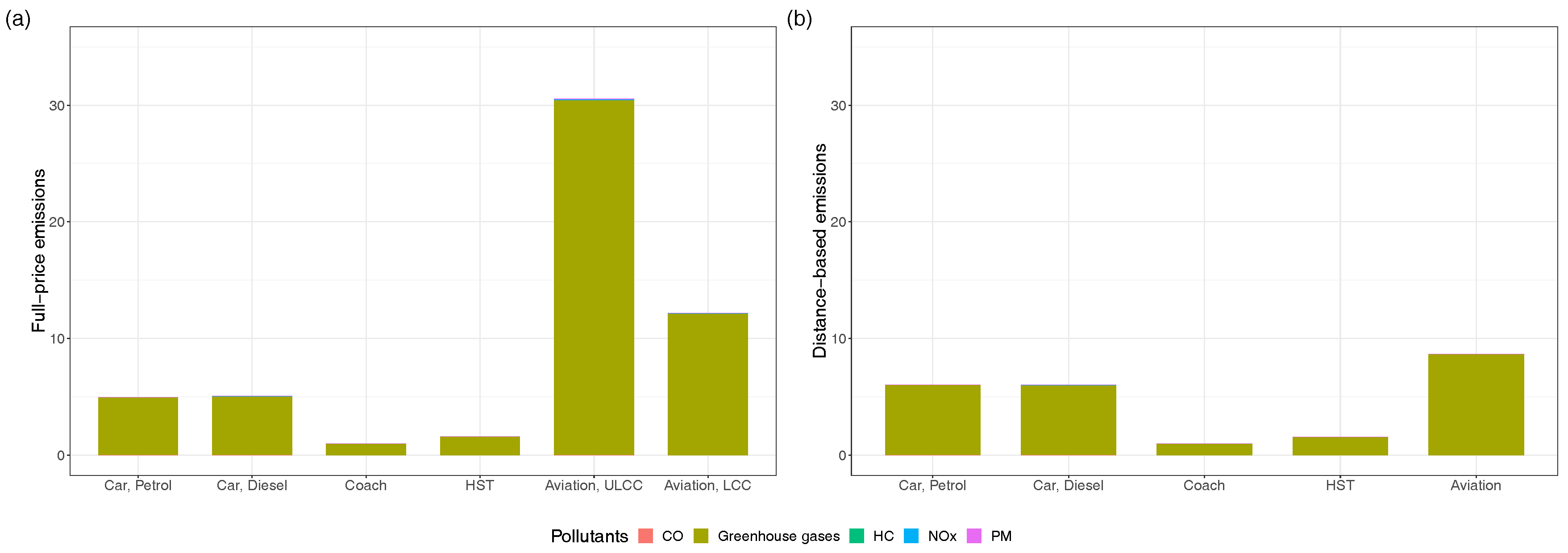
In the previous sections, we analysed the different scenarios separately. That is, we investigated the level of emissions for business trips on specific routes and then applied the methodological approach of full-price emissions so as to calculate emissions for holiday trips. The same procedure was applied when determining environmental costs. What remains in the end, is to calculate the (relative) metric for full-price emissions and to compare it with the emission factors which represent the traditional distance-based approach. The two metrics have the following potential interpretations: on the one hand, the average emissions per person and Euro full-price invested are measured and on the other hand, the average emissions per person and kilometer. The results are displayed in Figure 10, where the metric for the most environmentally friendly transport mode (coach) is normalized to 1. It is clear that, in the case of full-price emissions, the climate disadvantage of aviation is much more pronounced. In the extreme scenario (Aviation, ULCC), the climate disadvantage of aviation is larger than 30, compared to coaches. In the moderate scenario (Aviation, LCC), the climate disadvantage is still at a high level with a factor of 12 (see Figure 10a). By comparison, for the traditional approach, the factor amounts to 8 (see Figure 10b). For all other transport modes (except HST), the relative climate damage declines when considering full-price emissions due to higher travel-cost factors and/or lower average speeds. Average emissions per person and Euro full price are lowest for coaches. If we look at the “family scenario”, it can be concluded that family travel improves the environmental performance of cars, whereas other transport modes are not affected (see Appendix D, Figure A3).
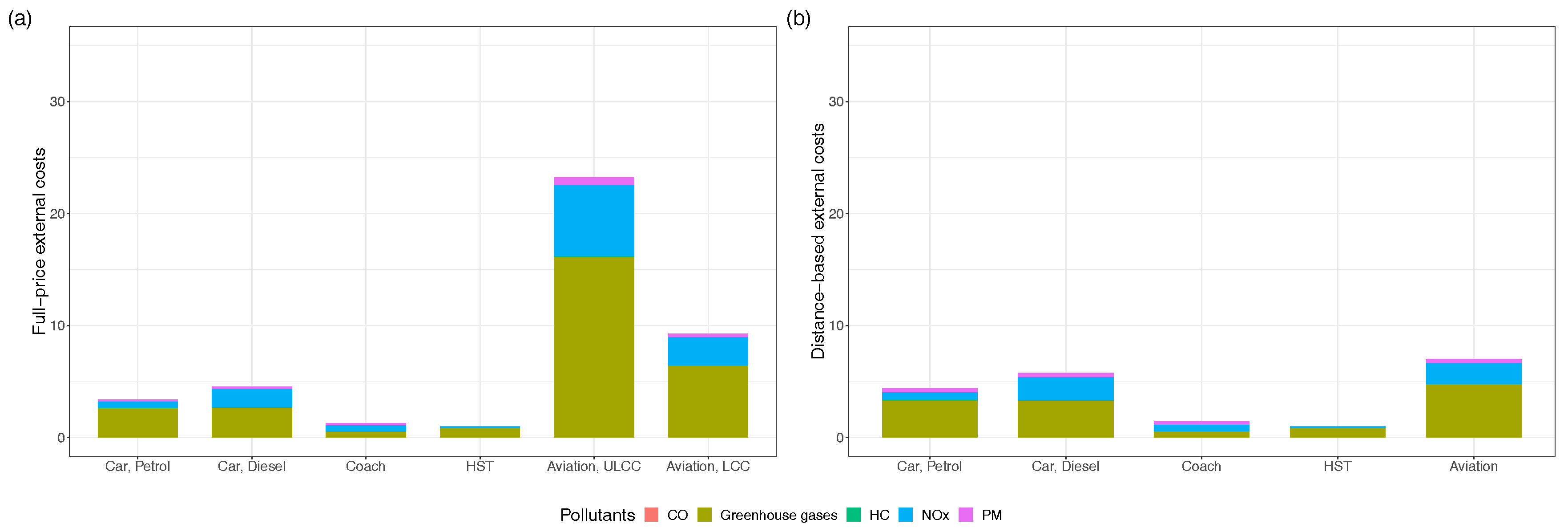
If we apply this comparison to environmental costs, the results change in that HST exhibit the lowest external costs per person and Euro full-price, for the reasons explained in Section 4.2, as for example, resulting from the interplay between the level of damage-cost factors and the level of emissions of different pollutants. The environmental cost advantage of HST amounts to a factor of 9 (moderate scenario, LCC) to 23 (extreme scenario, ULCC), compared to a factor of 7 when applying the traditional approach (see Appendix E).
5. Discussion
In general, our results confirm prior research in this field, as stated in Section 2. Nevertheless, some differences should be mentioned. For example, the German Transport Club [7] employs an analysis of CO2 emissions on the Berlin-Frankfurt link. The link can be characterized as a typical business trip and thus represents the traditional approach for determining emissions, where destinations remain exogenous. Whereas the German Transport Club finds that car emissions on this link are highest, followed by emissions from aviation [7], our results, by contrast, show a different environmental performance ranking. CO2 emissions are highest for aviation, regardless of the travel purpose. The main reason is that we use average emission factors that include a Radiative Forcing Index, which takes the greater greenhouse gas effects of aviation into consideration, whereas the German Transport Club ignores this effect. It should be mentioned that there is an ongoing debate on the contribution of aviation to radiative forcing. For example, Righi et al. [36] show that there might be negative effects for aviation with respect to aerosol radiative forcing. However, several other studies indicate that aviation rather contributes to a positive radiative forcing of climate than not (see e.g., References [37,38,39]), which is why we use factors that include a Radiative Forcing Index. Moreover, we show that the extent of the climate disadvantage of aviation increases significantly, if we look at full-price emissions. This is the consequence of the approach which incorporates a decision-making process. As we argue, holiday/leisure travellers determine a budget of money and time for holiday trips and thus implicitly for transport. Consequently, destinations become endogenous and thus distances can differ between transport modes. Therefore, transport modes which are characterized by low average ticket prices and high average speeds, both of which apply to aviation, achieve larger distances. And since aviation has also the highest average emission factor, aviation emissions increase significantly.
CE Delft [4] and the German Environment Agency [6] estimate the environmental costs of transport modes and find that these are highest for aviation and lowest for coaches. Our own study is thus in line with these findings. Additionally, our study emphasizes that environmental costs are significantly higher if we consider full-price emissions.
As passenger transport accounts for more than half of total CO2 emissions from the transport sector and several other pollutant emissions, environmental policies designated for the (passenger) transport sector have become an important issue in mitigating global climate change. From a theoretical point of view, an emissions trading system including the transport sector as well as an overall CO2 tax are appropriate environmental policy instruments. In reality, however, policy measures focusing on single transport modes are commonly discussed. While these measures may get closer to 1st-best pricing from a transport-mode-specific perspective, environmental effects of the passenger transport sector can worsen, due to suboptimal pricing of other transport modes, that is, deviations from 1st-best pricing [40]. Consequently, the 2nd-best solution is to determine the optimal price for emissions subject to the constraint that alternative transport modes are not priced at 1st best [41]. Therefore, if measures focus on single transport modes, economic theory suggests substitution effects to occur. If the price of one transport mode rises (e.g., due to higher environmental taxes), consumers might simply choose another mode of transport. As suggested by full-price emissions, a holiday trip by car (to the Baltic Sea), for example, may then be substituted for a holiday trip by air (to Mallorca). This would imply an increase in environmental pollution by a factor of 6 to 7 (moderate scenario factor 3). However, these effects are often ignored in the political debate. One possible explanation for this is that the established comparisons of emissions between transport modes (which are distance-based) ignore substitution effects, because price is not a decision variable. Consequently, our approach is able to model potential effects of environmental policies, such as a CO2 tax but comes at the cost of restricted applicability. More specifically, applying this approach to countries with a different environmental policy is not possible, as full-price emissions depend on the (environmental) policy and thus respond to a change in policy. By contrast, the distance-based metric focuses on a “technically” correct estimation of emissions and thus the transport mode decision and therefore the destination/distance remain exogenous. Thus, it might represent emissions of business trips adequately but may well fail for travel where destinations are determined endogenously and consequently the price is part of the decision-making process.
6. Conclusions
We use a full-price emissions approach to estimate emissions accruing from holiday trips. The results show that the relative climate damage of aviation is much more pronounced when destinations are endogenous, compared to when they are exogenous. This result is in particular determined by the endogeneity of destinations. Considering fixed full-price budgets, consumers can travel larger distances by air, because on the one hand, lower ticket prices and on the other hand lower travel times, apply. This is also influenced by intense intramodal competition in the aviation sector. Furthermore, it can be observed that the relative climate damage of aviation increases with the budget (up to the point where distances exceed the medium-haul threshold, because lower emission factors then apply). Thus, lower budgets imply a less pronounced relative climate disadvantage of aviation. This can be explained partly by the higher share of time costs from check-in and out processes in the total full-price budget, which decrease viable distances.
We further observe that differences in emissions between petrol and diesel cars are rather low. Given that diesel cars were promoted as more environmentally friendly, it should be expected that they emit significantly less emissions than petrol cars. However, if we take well-to-tank emissions into account, the emissions of the average petrol car compared to the average diesel car are approximately equal. Full-price emissions even show that the environmental performance of petrol cars is better than that of diesel cars. The results are driven by higher greenhouse gas emissions from fuel production (higher well-to-tank emissions), higher NOX emissions and lower travel-cost factors of diesel cars (due to lower fuel prices). Moreover, the analysis of a “family scenario” reveals that cars benefit significantly from higher occupation. That is, car emissions per person decrease, as the positive effect on the average emission factors overcompensates the negative effect on travel costs per pkm.
Although our research does not provide real-time emissions data, it develops a methodology to evaluate emissions for holiday trips, in which a decision-making process including a price variable is incorporated. Consequently, policy measures can be evaluated. In particular, it becomes obvious that policy measures (especially measures which affect pricing and taxation) have to be evaluated taking into account all possible effects (which differ between travel purposes) in order to avoid unintended and climate-damaging substitution effects. In this way, full-price emissions can serve as the appropriate instrument.
Author Contributions
T.H. contributed to all aspects of the paper (research design, methodological choices, analysis) and wrote the manuscript text; G.S. provided the idea of full-price emissions, supervision and a critical revision of the manuscript.
Funding
This research received no external funding.
Acknowledgments
The author would like to thank two anonymous referees for helpful comments, Christina Brand for her helpful comments and suggestions contributing to this research paper, Jan Wessel for a critical revision of the manuscript, and Brian Bloch for his editing services.
Conflicts of Interest
The authors declare no conflicts of interest.
Abbreviations
The following abbreviations are used in this manuscript:
| COPERT | Computer Programme for calculating Emissions from Road Transport |
| CO | Carbon monoxide |
| EUR | Euros |
| g | Grams |
| GWP | Global Warming Potentials |
| HBEFA | Handbook of Road Transport Emissions Factors |
| HC | Hydrocarbon |
| HST | High-speed train |
| kg | Kilograms |
| LCC | Low-cost carrier |
| NOX | Nitrogen oxide |
| pkm | Person-kilometers/ passenger kilometers |
| PM | Particulate matter |
| TREMOD | Transport Emission Model |
| ULCC | Ultra-low cost carrier |
Appendix A
Figure A1.
Development of Passenger kilometers in EU-28 [2].
Figure A1.
Development of Passenger kilometers in EU-28 [2].

Appendix B

Table A1.
Distance-based travel-time cost factors [27].
Table A1.
Distance-based travel-time cost factors [27].
| Distance (km) | (€ Per Person and Hour) |
|---|---|
| ⋮ | ⋮ |
| 45 | 8.17 |
| 55 | 8.70 |
| ⋮ | ⋮ |
| 95 | 10.20 |
| 112.5 | 10.66 |
| 137.5 | 11.18 |
| 162.5 | 11.82 |
| 187.5 | 12.24 |
| 212.5 | 12.53 |
| 275 | 12.79 |
| 325 | 13.17 |
| 375 | 13.71 |
| 425 | 14.07 |
| 475 | 14.42 |
| 600 | 14.77 |
| >600 | 15.54 |
Table A2.
Input factors used for calculating full-price emissions.
| Vehicle Type | Average Speed (km/h) | Travel-Cost Factor (€/pkm) | Full-Price Factor (€/pkm) a |
|---|---|---|---|
| Car, Petrol | 82.16 | 0.1412 | 0.3303 |
| Car, Diesel | 82.16 | 0.1345 | 0.3236 |
| Coach | 79.39 | 0.0740 | 0.2697 |
| HST | 110.00 | 0.1094 | 0.2507 |
| Aviation, ULCC (Ryanair) | 522.19 | 0.0334 | 0.0632 |
| Aviation, LCC (Eurowings) | 522.19 | 0.1289 | 0.1586 |
a Full-price factor for distances > 600 km.
Table A3.
Damage-cost factors of air pollutants (€/t) [27].
Appendix C
Calculation of weighted marginal external cost factors:
Table A4.
Breakdown of mileage by vehicle category a [5].
Table A4.
Breakdown of mileage by vehicle category a [5].
| Transport Mode | Urban | Suburban | Rural | Motorway |
|---|---|---|---|---|
| Car | 0.26 | 0.205 | 0.205 | 0.33 |
| Coach | 0.09 | 0.29 | 0.29 | 0.34 |
| HST b | 0.1942 | 0.3503 | 0.4431 | 0.0000 |
| Aviation | no differentiation across road types | |||
a We divide the share of kilometers travelled out of town equally between suburban und rural; b For HST no data were available. Thus, we rely on our own calculations performed with Qgis. We used Census data for population densities and then manually mapped routes (using OSM) for several German long-distance tracks to obtain the kilometers driven within each regional/road area.
In order to calculate (weighted) marginal external cost factors of road transport, we assume average size fleets. Thus, we determine the share of cars in the vehicle stock across each emission class. We consider cars of medium size (1.4–2.0 l). The number of cars in the vehicle stock is reported by the German Federal Office for Motor Transport (Kraftfahrt-Bundesamt) [42]. We then convert the figures into relative shares (see Table A5), which enable us to calculate an average vehicle type emission factor.
Table A5.
Share of vehicles according to emission classes in the vehicle stock in Germany 2018 [42].
Table A5.
Share of vehicles according to emission classes in the vehicle stock in Germany 2018 [42].
| Emission Class | ||||||
|---|---|---|---|---|---|---|
| Vehicle Type | EURO I | EURO II | EURO III | EURO IV | EURO V | EURO VI |
| Car, Medium, Petrol | 0.0300 | 0.1496 | 0.1105 | 0.3905 | 0.1737 | 0.1457 |
| Car, Medium, Diesel | 0.0036 | 0.0204 | 0.0872 | 0.2170 | 0.4049 | 0.2668 |
| Buses/Coaches | 0.0 | 0.0 | 0.1949 | 0.0848 | 0.3896 | 0.3307 |
Table A6.
(Weighted) Marginal external cost factors.
| Vehicle Type | Air Pollution a | Climate Change | Well-to-Tank |
|---|---|---|---|
| (€-Cent/pkm) | (€-Cent/pkm) | (€-Cent/pkm) | |
| Car, Petrol | 0.1351 | 1.1006 | 0.4144 |
| Car, Diesel | 0.7627 | 1.1528 | 0.2689 |
| Coach | 0.3807 | 0.4719 | 0.1094 |
| HST | 0.0020 | 0.0000 | 0.3900 |
| Aviation, Short Haul | 0.2900 | 3.1400 | 1.3500 |
| Aviation, Medium Haul | 0.0900 | 1.8550 | 0.6000 |
a Metropolitan area is not considered.
Appendix D
Results for a “familiy scenario” (= four persons):
- Emissions on a holiday trip:
Figure A2.
Holiday trips – “family scenario”. (a) Emissions for ; (b) Emissions for .

- Comparison between full-price emissions and distance-based emissions:
Figure A3.
“Family scenario”. (a) Full-price emissions; (b) Distance-based emissions.

Appendix E
Comparison between full-price external costs and distance-based external costs:
Figure A4.
(a) Full-price (external) environmental costs; (b) Distance-based (external) environmental costs.
Figure A4.
(a) Full-price (external) environmental costs; (b) Distance-based (external) environmental costs.

References
- International Energy Agency. CO2 Emission Statistics. Available online: https://www.iea.org/statistics/co2emissions/ (accessed on 8 August 2019).
- European Environment Agency. Passenger Transport Volume and Modal Split. Available online: https://www.eea.europa.eu/data-and-maps/daviz/passenger-transport-volume-5 (accessed on 26 August 2019).
- European Environment Agency. Energy Efficiency and Specific CO2 Emissions. Available online: https://www.eea.europa.eu/data-and-maps/indicators/energy-efficiency-and-specific-co2-emissions/energy-efficiency-and-specific-co2-9 (accessed on 29 November 2019).
- Van Essen, H.; van Wijngaarden, L.; Schroten, A.; Sutter, D.; Bieler, C.; Maffii, S.; Brambilla, M.; Fiorello, D.; Fermi, F.; Parolin, R.; et al. Handbook on the External Costs of Transport; European Commission: Delft, The Netherlands, 2019. [Google Scholar]
- Matthey, A.; Bünger, B. Methodological Convention 3.0 for the Assessment of Environmental Costs-Cost Rates; Umweltbundesamt: Dessau-Roßlau, Germany, 2019.
- Umweltbundesamt. Vergleich der Durchschnittlichen Emissionen Einzelner Verkehrsmittel im Personenverkehr. Available online: https://www.umweltbundesamt.de/bild/vergleich-der-durchschnittlichen-emissionen-0 (accessed on 2 September 2019).
- Verkehrsclub Deutschland. Intelligent Mobil-Verkehrsmittel im Vergleich. Available online: https://www.vcd.org/themen/klimafreundliche-mobilitaet/verkehrsmittel-im-vergleich/ (accessed on 26 September 2019).
- González-Savignat, M. Competition in Air Transport—The Case of the High Speed Train. J. Transp. Econ. Policy 2004, 38, 77–108. [Google Scholar]
- Hagedorn, T.; Sieg, G. Treibhausgasemissionen im fahrzweckbezogenen Verkehrsmittelvergleich. Int. Verkehrswesen 2019, 71, 56–60. [Google Scholar]
- Kidokoro, Y.; Zhang, A. Airport congestion pricing and cost recovery with side business. Transp. Res. Part A 2018, 114, 222–236. [Google Scholar] [CrossRef]
- Zhang, A.; Zhang, Y. Airport capacity and congestion when carriers have market power. J. Urban Econ. 2006, 60, 229–247. [Google Scholar] [CrossRef]
- infas; DLR; IVT; infas360. Mobilität in Deutschland-MiD Ergebnisbericht; Bundesministerium für Verkehr und digitale Infrastruktur: Bonn, Germany, 2019.
- Adler, N.; Pels, E.; Nash, C. High-speed rail and air transport competition: Game engineering as tool for cost-benefit analysis. Transp. Res. Part B 2010, 44, 812–833. [Google Scholar] [CrossRef]
- Quarks. CO2-Rechner für Auto, Flugzeug und Co. Available online: https://www.quarks.de/umwelt/klimawandel/co2-rechner-fuer-auto-flugzeug-und-co/ (accessed on 5 September 2019).
- Karlsruher Institut für Technologie. Deutsches Mobilitätspanel (MOP)-Wissenschaftliche Begleitung und Auswertungen Bericht 2017/2018: Alltagsmobilität und Fahrleistung; Bundesministerium für Verkehr und digitale Infrastruktur: Karlsruhe, Germany, 2019.
- Edwards, R.; Larivé, J.-F.; Rickeard, D.; Weindorf, W. Well-To-Tank Report Version 4a; European Commission: Luxembourg, 2014. [Google Scholar]
- Umweltbundesamt. Emissionskennzahlen Datenbasis 2017. Available online: https://www.umweltbundesamt.at/fileadmin/site/umweltthemen/verkehr/1_verkehrsmittel/EKZ_Fzkm_Verkehrsmittel.pdf (accessed on 27 September 2019).
- MKC Consulting; IVT; INFRAS. HBEFA Version 3.3; Hintergrundbericht: Bern, Switzerland, 2017. [Google Scholar]
- Kumar Pathak, S.; Sood, V.; Singh, Y.; Channiwala, S.A. Real world vehicle emissions: Their correlation with driving parameters. Transp. Res. Part D 2016, 44, 157–176. [Google Scholar] [CrossRef]
- Kraftfahrt-Bundesamt. Verkehr in Kilometern. Available online: https://www.kba.de/DE/Statistik/Kraftverkehr/VerkehrKilometer/pseudo_verkehr_in_kilometern_node.html (accessed on 17 October 2019).
- European Commission. Commission Regulation (EU) No 459/2012; European Commission: Brussels, Belgium, 2012. [Google Scholar]
- Eisenkopf, A.; Hahn, C.; Schnöbel, C. Marktabgrenzung und Wettbewerb im Personenverkehr-zur Bedeutung des intermodalen Wettbewerbs aus der Perspektive des Schienenpersonenverkehrs. Z. für Verkehrswissenschaft 2008, 79, 35–73. [Google Scholar]
- Behrens, C.; Pels, E. Intermodal competition in the London-Paris passenger market: High-Speed Rail and air transport. J. Urban Econ. 2012, 71, 278–288. [Google Scholar] [CrossRef] [Green Version]
- Notter, B.; Wüthrich, P.; Heidt, C.; Knörr, W.; Melios, G.; Papadimitriou, G.; Kouridis, C. Vergleich COPERT—TREMOD; Bundesanstalt für Straßenwesen: Bergisch Gladbach, Germany, 2016.
- Wilkerson, J.T.; Jacobson, M.Z.; Malwitz, A.; Balasubramanian, S.; Wayson, R.; Fleming, G.; Naiman, A.D.; Lele, S.K. Analysis of emission data from global commercial aviation: 2004 and 2006. Atmos. Chem. Phys. 2010, 10, 6391–6408. [Google Scholar] [CrossRef] [Green Version]
- Kirnich, P. Fernbus vs. Bahn—Fernbusse: Günstig, Aber Langsamer. Berliner Zeitung, 15 September 2013. [Google Scholar]
- PTV Group. Methodenhandbuch zum Bundesverkehrswegeplan 2030; Bundesministerium für Verkehr und digitale Infrastruktur: Bonn, Germany, 2016.
- Steer Davies Gleave. Study on the Prices and Quality of Rail Passenger Services; European Commission, Directorate General for Mobility and Transport: Brussels, Belgium, 2016. [Google Scholar]
- Statista. Entwicklung der Kilometerpreise für Fernbuskunden in Deutschland von 2002 bis 2018. Available online: https://de.statista.com/statistik/daten/studie/380601/umfrage/kilometerpreise-fernbuslinien-in-deutschland/ (accessed on 20 September 2019).
- DB Fernverkehr AG. Stellungnahme der DB Fernverkehr AG Anlässlich der Öffentlichen Anhörung des Ausschusses für Verkehr und Digitale Infrastruktur des Deutschen Bundestages am 15. Februar 2017; Deutscher Bundestag, Ausschuss für Verkehr und digitale Infrastruktur: Bonn, Germany, 2017.
- ADAC. ADAC Autokosten. Available online: https://www.adac.de/infotestrat/autodatenbank/autokosten/ (accessed on 10 September 2019).
- Intraplan Consult GmbH; Planco Consulting GmbH, TUBS GmbH. Grundsätzliche Überprüfung und Weiterentwicklung der Nutzen-Kosten-Analyse im Bewertungsverfahren der Bundesverkehrswegeplanung; Bundesministerium für Verkehr und digitale Infrastruktur: Bonn, Germany, 2015.
- McGuckin, N.; Fucci, A. Summary of Travel Trends: 2017 National Household Travel Survey; U.S. Department of Transportation: Washington, DC, USA, 2018.
- Scottish Government. Private Transport—Car Occupancy. Available online: https://www2.gov.scot/Topics/Statistics/Browse/Transport-Travel/TrendCarOccupancy (accessed on 28 November 2019).
- European Environment Agency. Occupancy Rates. Available online: https://www.eea.europa.eu/publications/ENVISSUENo12/page029.html (accessed on 28 November 2019).
- Righi, M.; Hendricks, J.; Sausen, R. The global impact of the transport sectors on atmospheric aerosol: Simulations for year 2000 emissions. Atmos. Chem. Phys. 2013, 13, 9939–9970. [Google Scholar] [CrossRef] [Green Version]
- Penner, J.E.; Lister, D.H.; Griggs, D.J.; Dokken, D.J.; McFarlandm, M. Aviation and the Global Atmosphere—Summary for Policymakers; Intergovernmental Panel on Climate Change: Geneva, Switzerland, 1999. [Google Scholar]
- Sausen, R.; Isaksen, I.; Grewe, V.; Hauglustaine, D.; Lee, D.S.; Myhre, G.; Köhler, M.O.; Pitari, G.; Schumann, U.; Stordal, F.; et al. Aviation radiative forcing in 2000: An update on IPCC (1999). Metereologische Z. 2005, 14, 555–561. [Google Scholar] [CrossRef] [PubMed] [Green Version]
- Lee, D.S.; Fahey, D.W.; Forster, P.M.; Newton, P.J.; Wit, R.C.N.; Lim, L.L.; Owen, B.; Sausen, R. Aviation and global climate change in the 21st century. Atmos. Environ. 2009, 43, 3520–3537. [Google Scholar] [CrossRef] [Green Version]
- Tscharaktschiew, S. Shedding light on the appropriateness of the (high) gasoline tax level in Germany. Econ. Transp. 2014, 3, 189–210. [Google Scholar] [CrossRef]
- O’Flaherty, B. City Economics; Harvard University Press: London, UK, 2005. [Google Scholar]
- Kraftfahrt-Bundesamt. Fahrzeugzulassungen-Bestand an Kraftfahrzeugen nach Umwelt-Merkmalen; Kraftfahrt-Bundesamt: Flensburg, Germany, 2018.
Figure 1.
Share of passenger kilometers in Germany in 2017 related to different travel purposes [12].
Figure 1.
Share of passenger kilometers in Germany in 2017 related to different travel purposes [12].

Figure 2.
(a) Average external environmental costs (in €-Cent/pkm); (b) Marginal external environmental costs (in €-Cent/pkm); (c) Total external environmental costs 2016 for EU28 (in Billions € per year) [4]. Different scales are used. For marginal costs the following vehicle types were assumed: Car, Petrol, Medium, 1.4–2.0 l, EURO V; Car, Diesel, Medium, 1.4–2.0 l, EURO V; Coach, Diesel, Standard <= 18 t, EURO V; High-speed train; Aviation, Short Haul.

Figure 3.
Business-trip emissions (a) on the Cologne-Berlin link; (b) on the Hamburg-Munich link. Emissions of CO, HC, NOX and PM are so low (relative to greenhouse gases) that they are nearly insignificant, and thus invisible.
Figure 3.
Business-trip emissions (a) on the Cologne-Berlin link; (b) on the Hamburg-Munich link. Emissions of CO, HC, NOX and PM are so low (relative to greenhouse gases) that they are nearly insignificant, and thus invisible.

Figure 4.
Holiday-trip emissions (a) for ; (b) for . Emissions of CO, HC, NOX and PM are so low (relative to greenhouse gases) that they are nearly insignificant, and thus invisible.
Figure 4.
Holiday-trip emissions (a) for ; (b) for . Emissions of CO, HC, NOX and PM are so low (relative to greenhouse gases) that they are nearly insignificant, and thus invisible.

Figure 5.
Maximum transport-mode-specific distances for .

Figure 6.
Business trips. (a) (External) environmental costs on the Cologne-Berlin link; (b) (External) environmental costs on the Hamburg-Munich link.
Figure 6.
Business trips. (a) (External) environmental costs on the Cologne-Berlin link; (b) (External) environmental costs on the Hamburg-Munich link.

Figure 7.
Holiday trips. (a) (External) environmental costs for ; (b) (External) environmental costs for .
Figure 7.
Holiday trips. (a) (External) environmental costs for ; (b) (External) environmental costs for .

Figure 8.
Business trips. (a) (External) environmental costs on the Cologne-Berlin link, (b) (External) environmental costs on the Hamburg-Munich link (on the basis of Reference [4]).
Figure 8.
Business trips. (a) (External) environmental costs on the Cologne-Berlin link, (b) (External) environmental costs on the Hamburg-Munich link (on the basis of Reference [4]).

Figure 9.
Holiday trips. (a) (External) environmental costs for , (b) (External) environmental costs for (on the basis of Reference [4]). In (b) external costs of ultra-low cost carriers (ULCCs) consider a medium-haul flight and are therefore lower.
Figure 9.
Holiday trips. (a) (External) environmental costs for , (b) (External) environmental costs for (on the basis of Reference [4]). In (b) external costs of ultra-low cost carriers (ULCCs) consider a medium-haul flight and are therefore lower.

Figure 10.
(a) Full-price emissions; (b) Distance-based emissions. Emissions of CO, HC, NOX and PM are so low (relative to greenhouse gases) that they are nearly insignificant, and thus invisible.
Figure 10.
(a) Full-price emissions; (b) Distance-based emissions. Emissions of CO, HC, NOX and PM are so low (relative to greenhouse gases) that they are nearly insignificant, and thus invisible.

Table 1.
Average emission factors (in g/pkm) of different transport modes.
| Pollutant | Car, Petrol | Car, Diesel | Coach a | Long-Distance Train | Aviation |
|---|---|---|---|---|---|
| Greenhouse gases | 139 b | 139 c | 23 | 36 | 201 |
| CO | 0.80 d | 0.39 d | 0.04 | 0.02 | 0.13 |
| HC | 0.14 | 0.14 | 0.01 | 0.00 | 0.04 |
| NOX | 0.19 b | 0.56 c | 0.17 | 0.04 | 0.51 |
| PM | 0.004 | 0.004 | 0.003 | 0.000 | 0.004 |
| ∑/Emission factor | 140.134 | 140.164 | 23.223 | 36.060 | 201.684 |
| Load factor | 1.5 Pers./Car | 1.5 Pers./Car | 60 % | 56 % | 83 % |
a Coaches contain occasional as well as scheduled transport services. For greenhouse gases, only emission factors of scheduled transport services are considered [14]; b Car, Petrol, Medium, Average fuel consumption: 7.5 l/100 km [15]; c Car, Diesel, Medium, Average fuel consumption: 6.6 l/100 km [15]; d Emission factors are calculated on the basis of the mean value published by the German Environment Agency. We assume that these are approximately evenly distributed around the mean for petrol and diesel cars, thereby taking into account the share of passenger kilometers made by both vehicle types.
Table 2.
Marginal air pollution costs for EU28 in 2016, in €-Cent per pkm.
| Vehicle | Specification | Metropolitan Area a | Urban Area a | Rural Area a |
|---|---|---|---|---|
| Car, Petrol | 1.4–2.0 l, EURO V | 0.117 | 0.100 | 0.075 |
| Car, Diesel | 1.4–2.0 l, EURO V | 0.903 | 0.945 | 0.500 |
| Coaches, Diesel | Standard ≤ 18 t, EURO V | 0.940 | 1.015 | 0.250 |
| HST | Electric | 0.010 | 0.010 | 0.010 |
| Aviation, Short Haul | 0.290 b | |||
a Values are averaged over different road types (Motorway, Urban/Rural roads); b Values are not differentiated across regional areas.
Table 3.
Marginal climate change costs for EU28 in 2016, in €-Cent per pkm.
| Vehicle | Specification | Metropolitan Area | Urban Area | Other Area |
|---|---|---|---|---|
| Car, Petrol | 1.4–2.0 l, EURO V | 1.11 | 1.29 | 1.02 |
| Car, Diesel | 1.4–2.0 l, EURO V | 1.18 | 1.31 | 1.03 |
| Coaches, Diesel | Standard ≤ 18 t, EURO V | 0.40 | 0.80 | 0.44 |
| HST | Electric | 0.00 | 0.00 | 0.00 |
| Aviation, Short Haul | 3.14 a | |||
a Values are not differentiated across regional areas. Average value for two different aircraft types.
Table 4.
Marginal costs of well-to-tank emissions for EU28 in 2016, in €-Cent per pkm.
| Vehicle | Specification | Motorway | Urban Road | Other Road |
|---|---|---|---|---|
| Car, Petrol | 1.4–2.0 l, EURO V | 0.42 | 0.49 | 0.38 |
| Car, Diesel | 1.4–2.0 l, EURO V | 0.28 | 0.30 | 0.24 |
| Coaches, Diesel | Standard ≤ 18 t, EURO V | 0.09 | 0.19 | 0.10 |
| HST | Electric | 0.39 a | ||
| Aviation, Short Haul | 1.35 b | |||
a Values are not differentiated across regional areas; b Values are not differentiated across regional areas. Average value for two different aircraft types.
© 2019 by the authors. Licensee MDPI, Basel, Switzerland. This article is an open access article distributed under the terms and conditions of the Creative Commons Attribution (CC BY) license (http://creativecommons.org/licenses/by/4.0/).
Share and Cite
MDPI and ACS Style
Hagedorn, T.; Sieg, G. Emissions and External Environmental Costs from the Perspective of Differing Travel Purposes. Sustainability 2019, 11, 7233. https://0-doi-org.brum.beds.ac.uk/10.3390/su11247233
AMA Style
Hagedorn T, Sieg G. Emissions and External Environmental Costs from the Perspective of Differing Travel Purposes. Sustainability. 2019; 11(24):7233. https://0-doi-org.brum.beds.ac.uk/10.3390/su11247233
Chicago/Turabian StyleHagedorn, Thomas, and Gernot Sieg. 2019. "Emissions and External Environmental Costs from the Perspective of Differing Travel Purposes" Sustainability 11, no. 24: 7233. https://0-doi-org.brum.beds.ac.uk/10.3390/su11247233
Note that from the first issue of 2016, this journal uses article numbers instead of page numbers. See further details here.