On the Pricing of Urban Rail Transit with Track Sharing Freight Service

Abstract

Transporting parcels on urban passenger rail transit is gaining growing interest as a response to the increasing demand and cost of urban parcel delivery. To analyze the welfare effects of different fare regimes when allowing parcel services on an urban rail transit, this paper models the optimal service problem where the transit operator chooses the number of trains and the departure intervals. By introducing a reduced form train timetable problem, the passenger train crowding model is extended to incorporate the effect of freight train scheduling. We show that the freight users are better off in the time-varying optimal fare regime, while passengers are worse off, and that the time-varying optimal fare regime calls for more trains than the optimal uniform fare regime. However, the reduction in passenger trains due to the introduction of freight service can eliminate the welfare gain from passenger time-varying fare. If the price elasticity of freight demand is relatively high, implementing road toll can generate welfare loss when rail transit is privately operated.

1. Introduction

Parcel delivery demand boosted by online retail incurs greater congestion, emission and labor cost [1,2]. As a response to the challenge, more initiatives are focusing on moving parcels on passenger rail transit (see Diziain et al. [3] and Cochrane et al. [4] for the reviews of recent practices). Kikuta et al. [5] report a survey resulting from a pilot project of freight on subway implemented in Japan. Positive feedback from various stakeholders are received. Intergrated transit systems have also been proposed to meet dynamic demand of both passenger and freight (e.g., Fatnassi et al. [6]). In most practices and studies, passenger and freight services are planned to be provided in designated time intervals, usually with passenger service in priority. The welfare effects of deciding such time intervals have not explored in depth.

The objective of this paper is to analyze the welfare effects of rail transit pricing when the freight on transit (FOT) service is provided. In particular, our analysis focuses on two questions, one concerning equity between user groups and the other optimal capacity. First, how does the time-varying transit fare affect the consumer surplus of passenger and freight users? Are they better off or worse off than in a flat fare regime? Second, does the freight service affect the optimal service capacity? Is it the case that, as when only passenger service is provided, more trains are needed when a time-varying fare is implemented?

The problem of optimal scheduling for mixed types of trains is usually treated separately in two stages. The first stage is to construct an optimal timetable for each type of train, typically with the objective to minimize the user scheduling cost or maximize the operating revenue (e.g., de Palma and Lindsey [7]). The second stage is to schedule (or path) different types of trains to minimize the deviation from the designated optimal timetable, subject to track and headway constraints (e.g., Carey and Lockwood [8], Carprara et al. [9], and Cacchiani and Toth [10]). As a variant of the second stage scheduling problem, Behiri et al. [11] develop a model for optimal train scheduling specifically in the context of FOT, assuming that the departure times of passenger trains are unaffected. Recently, Robenek et al. [12] made an effort to integrate the two stages of the optimal timetable problem, where the second stage of train scheduling also affects passengers’ departure time choice. However, passengers’ behavior of trading-off between crowding and scheduling cost is not considered in the above literature. The effects of freight service on passengers’ departure time choice are therefore not taken into account.

In contrast, dynamic model that accounts for road travelers trip-timing decision has been studied rigorously based on the bottleneck model introduced by Vickrey [13]. Analogous to a road bottleneck, Kraus and Yoshida [14] consider a bottleneck at the departure station. They assume that passengers have to wait for the next train if boarded passengers exceed train capacity, and that no late arrivals are allowed. In such cases, the departure time choice of passenger is made by trading scheduling cost due to early departures for queuing cost. Tian et al. [15] treat a more realistic scenario where the crowding cost varies with the number of boarded passengers. They also allow both early and late arrivals. The equilibrium cost of passengers then consists of crowding cost and scheduling cost. Recently, de Palma et al. [16] develop a more general model of passenger transit crowding. They discuss how the convexity of crowding cost function affects the welfare gain from introducing time-dependent fare. In addition, they find that rail transit requires more capacity investment in the social optimal fare regime, which contradicts with the conventional knowledge from road congestion pricing.

Our analysis builds on the previous works mainly in two ways. First, the two-stage optimal timetable problem is formulated in a reduce form, given the fact that the number of departure intervals is limited in the practices of FOT. The reduced form optimal timetable problem is then applied to extend the dynamic trip-timing models by de Palma et al. [16]. Second, we adopt the bottleneck model of road congestion (e.g., Vickrey [13] and Arnott et al. [17]) to model the queuing behavior of freight loading. By combining these two modeling features, we have a novel model that allows for an analysis of the optimal service problem where both the number and the departure time intervals of passenger trains are decided endogenously with that of freight trains. Our analysis parallels much of that in de Palma et al. [16], but is distinct in the following ways. We derive the optimal number of trains for both passenger and freight service type for four fare regimes: No-fare, optimal uniform-fare, optimal time-varying fare and private profit maximization fare. We highlight the welfare distributional effects between passenger and freight user, and remark the similarities and differences before and after the introduction of FOT service. The effect of an unpriced road as an alternative to rail transit is assessed, and the welfare loss due to private transit operation and unpriced road traffic is then compared as two types of market distortions. The role of scheduling preferences in welfare gain and the optimal service order is also discussed.

As the answer to the questions in the second paragraph, our results show that freight users are better off in the best time-varying fare regime, while passenger users are worse off. Therefore, a sophisticated fare rebate design is needed in order to achieve Pareto improvement. In the time-varying optimal fare regime, the total optimal number of total trains is higher than in the uniform fare regime. The number of passenger trains, however, can be lower, and the welfare gain from the time-varying fare of passengers can also be negative.

The layout of the paper is as follows. Section 2 reviews the passenger transit crowding model, and the conventional bottleneck model is adopted to capture the loading congestion of freight users in the departure station. The optimal timetable problem with fixed demand is treated in Section 3, and the problem is extended in Section 4 to consider elastic demand and the number of trains can be varied by the operator in the long run. In Section 6, numerical analysis is presented, and Section 7 concludes. A summary table of notations and proofs may be found in the Appendix.

2. A Model of Rail Transit Line with Track Sharing Services

In this section, we introduce a model of implementing freight service over a crowding rail transit line. Transit user type is indexed by $\eta =i,j$, where i for passenger and j for freight. The model of passenger crowding with only passenger service is firstly explained, followed by a model of freight loading congestion at the same departure station.

2.1. Passenger Service

Consider a single rail transit line connects the origin and the destination stations without intermediate stops. There are $m_i$ trains with the same capacity s operating over the line. As per a timetable, train k is scheduled to leave at $t_k,k=1,\cdots ,m_i$. The travel time T between the two stations is constant. A fixed number, $N_i$, of identical commuters take the line from home to work, and no other transportation modes are available. The situation is illustrated in Figure 1. The timetable information is fully available to the commuters, and the crowding costs $g\left(n_k\right)$ on train k, in terms of the discomfort of staying in a restricted space, are the same among boarded passengers $n_k$, i.e., no merit from early arrival in order to secure a more preferable place in the train. Then on each of train k, user incurs a crowding disutility $g\left(n_k\right)>0$. The boarding time is assumed independent of the number of boarding passengers, and is normalized to zero without loss of generality.

The limited capacity of a single train, from which the crowding cost stems, also entails scheduling cost for users. The dynamics of scheduling cost, introduced by Vickrey [18], is modeled with the assumption that the utility of one’s activity depends on the time spent on each place: Home and work. The total utility u gained by a user taking train k, usually has the following form:

$$u\left(t_k\right)={\int }_{t_h}^{t_k}h\left(t\right)dt+{\int }_{t_k+T}^{t_w}w\left(t\right)dt-g\left(n_k\right),$$

where $h\left(t\right)$ and $w\left(t\right)$ are the utility rate or Marginal Utility of Time (MUT) at time t when an individual being at home or at workplace, respectively. The constant $t_h$ denotes the start time of a day and $t_w$ the end time of work. Both function h and w are often assumed to be positive on their domains, and function h is non-increasing while w to be increasing, i.e., $h>0,h^{\prime }\le 0$ and $w>0,w^{\prime }>0$. The assumption is in line with the intuition that a trip to work is more beneficial to an individual than staying at home. Over the time of day being considered, the utility rate at work strictly increases from less to higher than the utility rate at home, before intersecting w at some time $t^{\ast }$. If there is a train scheduled to depart at $t^{\ast }$ with unlimited capacity, and travel time T is zero, all users would choose to take this train to arrive at the work place and achieve the maximum utility $u^{max}={\int }_{t_h}^{t^{\ast }}h\left(t\right)dt+{\int }_{t^{\ast }}^{t_w}w\left(t\right)dt$. Therefore $t^{\ast }$ is usually referred as the preferred arrival time (PAT). The scheduling cost of user i taking train k is therefore defined by

$${\delta }_i\left(t_k\right)=u^{max}-u\left(t_k\right)={\int }_{t_k}^{t^{\ast }}h\left(t\right)dt+{\int }_{t^{\ast }}^{t_k+T}w\left(t\right)dt.$$

(1)

When the train capacity is limited, and travel time is not zero, only users take the train departing at the the optimal departure time $t_k^{\ast }$ achieve the minimum scheduling cost, when they equalize the utility rate at home $h\left(t_k^{\ast }\right)$ and that at the workplace $w(t_k^{\ast }+T)$, as illustrated in Figure 2. In general, they suffer combined travel cost $c_i\left(t_k\right)={\delta }_i\left(t_k\right)+g\left(n_k\right),k=1,\cdots ,m_i$, where $n_k$ is the number of users boarded on the same train k. To simplify notations, ${\delta }_i\left(t_k\right)$ is written ${\delta }_{ik}$, and $c_i\left(t_k\right)$ is written $c_{ik}$.

In literature of departure time choice, two types of scheduling preferences have been utilized to represent the most common specifications for h and w, namely: Linear MUT and constant-step MUT (also known as $\alpha -\beta -\gamma$ preferences). Linear MUT preferences were introduced by Vickrey [18]. They have the formulation as follows: $h\left(t\right)={\beta }_0+{\beta }_{1}t$ and $w\left(t\right)={\gamma }_0+{\gamma }_{1}t$, with the assumption that ${\beta }_1\le 0$ and ${\gamma }_1>0$. The functions h and w intersect at the preferred arrival time $t^{\ast }=\frac{{\beta }_0-{\gamma }_0}{{\gamma }_1-{\beta }_1}$. The $\alpha -\beta -\gamma$ preferences were firstly introduced by Vickrey [13], and later restated by Tseng and Verhoef [19] by a constant function for h and a step function for w: $h\left(t\right)=\alpha ,w\left(t\right)=\alpha -\beta +(\beta +\gamma )·{𝟙}_{t\ge t_{\ast }}\left(t\right)$, where ${𝟙}_x$ is the indicator function with ${𝟙}_x=1$ if x is true, and ${𝟙}_x=0$ otherwise. Later in this subsection, we discuss the effect of scheduling preferences on welfare gain and the optimal service start time.

With travel cost defined, we are ready to introduce the departure time choice behavior in user equilibrium (UE). An extensive exposition of trip-timing decision in rail transit context is due to de Palma et al. [16]. Here we present mainly the result for better understanding the remaining text. Let the superscript e denote the no-fare user equilibrium. When no fare applied by the operator, users distribute themselves across trains by trading-off between scheduling cost ${\delta }_{ik}$ and crowding cost $g\left(n_k\right),k=1,\cdots$. When the equilibrium state established, the private travel cost of user on train k equals to the equilibrium cost

$$c_i^e={\delta }_k+g\left(n_k\right).$$

(2)

Since the crowding cost function depends on passengers’ preferences, the shape of $g\left(n\right)$ can differ between cities and user groups. To simplify the matters, the crowding cost throughout the text is assumed to be a linear function of boarded passengers on trains k, i.e., $g\left(n_k\right)=\lambda n_k/s$. (See de Palma et al. [16] for the effects of crowding cost function specification.) Define $\overline{{\delta }_i}\equiv \frac{1}{m_i}{\sum }_{k=1}^{m_i}{\delta }_{ik}$ as the average scheduling cost between train k. Using the identity ${\sum }_{k=1}^{m_i}{n}_k^e=N_i$, $n_k^e$ and $c_i^e$ can be derived by solving Equation (2):

$$\begin{array}{cc}\hfill n_k^e& =\frac{N_i}{m_i}+\frac{s}{\lambda }(\overline{{\delta }_i}-{\delta }_{ik}),\hfill \end{array}$$

(3)

$$\begin{array}{cc}\hfill c_i^e& =\overline{{\delta }_i}+\frac{\lambda N_i}{m_{i}s}.\hfill \end{array}$$

(4)

When the total number demand of passenger trip $N^i$ is inelastic, transit operator is not able to restrict transit usage by applying a uniform fares regime. The marginal social cost of a trip, $MS{C}_i$, is derived by differentiating the total equilibrium cost, $c_i^e{N}^i$, with respect to $N^i$:

$$MS{C}_i^e=\overline{{\delta }_i}+2\frac{\lambda N_i}{m_{i}s}.$$

(5)

Then elastic demand (as assumed in Section 4) can be regulated to the efficient level by an fare equal to the average marginal external cost:

$${\tau }_i^u=MS{C}_i^e-c_i^e=\frac{\lambda N_i}{m_{i}s},$$

(6)

where the superscript “u” denotes the optimal uniform fare regime. Then the total travel cost net of the fare in optimal uniform fare regime is:

$$T{C}_i^u=\overline{{\delta }_i}{N}_i+\frac{\lambda {\left(N_i\right)}^2}{m_{i}s}.$$

(7)

If the operator is allowed to charge train-dependent fare, users can then be distributed optimally between trains to minimize total travel cost. Let superscript o denote the social optimal (SO) fare regime, and the fare minimizes total travel cost is called SO-fare. Instead of a sum of equilibrium cost, the total travel cost is now given as $T{C}_i^o={\sum }_{k=1}^{m_i}{c}_{ik}{n}_k$. Treating ${\sum }_{k=1}^{m_i}{n}_k=N_i$ as the constraint of minimizing $T{C}_i^o$, the first order conditions gives that the marginal social cost of using each train k, $MS{C}_{ik}$ equals to the marginal social cost of a trip $MS{C}_i^o$:

$$MS{C}_{ik}=\frac{\partial c_{ik}{n}_k}{\partial n_k}={\delta }_{ik}+2\frac{\lambda }{s}{n}_k=MS{C}_i^o,$$

(8)

where

$$MS{C}_i^o=\frac{\partial T{C}_i^o}{\partial N_i}=\overline{{\delta }_i}+2\frac{\lambda N_i}{m_{i}s}.$$

(9)

Jointly solving Equations (8) and (9) for $n_k$ gives:

$$n_k^o=\frac{N_i}{m_i}+\frac{s}{2\lambda }(\overline{{\delta }_i}-{\delta }_{ik}).$$

(10)

Then the marginal external cost of usage, or the SO-fare is derived as

$${\tau }_{ik}^o=MS{C}_k-c_k=\frac{\lambda }{s}{n}_k^o.$$

(11)

Given Equations (10) and (11), total revenue from the SO-fare is

$$R_i^o=\sum _{k=1}^{m_i}{n}_k^o{\tau }_{ik}^o=\frac{\lambda }{m_{i}s}{N}_i^2+R{V}^o,$$

(12)

where

$$R{V}^o\equiv \frac{s}{4\lambda }\left(\sum _{k=1}^{m_i}{\delta }_{ik}^2-m_i{\overline{{\delta }_i}}^2\right).$$

(13)

By comparing Equations (6) and (12), it is easy to see that $R{V}^o$ is the variable part of revenue collecting from the time-varying SO-fare. Following de Palma et al. [16], we call it variable revenue. Now the total travel cost net of the SO-fare can be written as

$$T{C}_i^o=\overline{{\delta }_i}{N}_i+\frac{\lambda {N_i}^2}{m_{i}s}-R{V}^o,$$

(14)

where the first two terms are the total travel cost in UE, $T{C}_i^e=c_i^e{N}_i$; therefore, $R{V}^o$ gives the welfare gain from imposing SO-fare $G^{eo}$, defined as the difference of total travel cost between UE and SO fare regimes, i.e., $G^{eo}=R{V}^o=T{C}_i^e-T{C}_i^o$. Note that $R{V}^o$ is only a function of $m_i$ when all the trains are occupied. Since the train with the highest schedule delay cost has the lowest usage, the condition of minimum $N_i$ for all the trains are used in UE, and SO can be found by making Equations (3) and (10), respectively, positive for $max[{\delta }_1,{\delta }_{m_i}]$.

Next we show how scheduling preferences affect the way that the optimal service time $t_1^{\ast }$ and $R{V}^{o\ast }$ change with the number of trains $m_i$. For a given $m_i$, a public operator chooses a start time of the service that minimizes total travel cost. Assuming that the headway between trains is a constant h, it is straightforward to find the start time by differentiating $\overline{{\delta }_i}$ with respect to the departure time of first train $t_1$. With $t_1^{\ast }$ solved, the optimal value $\overline{{\delta }_i}$ and $R{V}^o$ are also decided. The results are summarized along with the specifications of scheduling preferences in

Table 1. Summary table of scheduling preferences, optimal service start time, optimal average schedule delay cost and optimal variable revenue.

	Linear MUT	Constant-Step MUT [16]
$h\left(t\right)$	${\beta }_0+{\beta }_{1}t$	$\alpha$
$w\left(t\right)$	${\gamma }_0+{\gamma }_{1}t$	$\alpha -\beta +(\beta +\alpha )·{𝟙}_{t\ge t^{\ast }}\left(t\right)$
$t_1^{\ast }$	$t^{\ast }-\frac{{\gamma }_1}{{\gamma }_1-{\beta }_1}T-\frac{(m-1)h}{2}$	$t^{\ast }-\left(\frac{\gamma m}{\beta +\gamma }+\frac{1}{2}\right)h$
${\overline{\delta }}^{\ast }$	≃$\frac{({\gamma }_1-{\beta }_1)h^2}{24}{m}^2$	$\simeq \frac{\beta \gamma }{\beta +\gamma }\frac{h}{2}m$
$R{V}^{o\ast }$	$\simeq \frac{({\gamma }_1-{\beta }_1)h^{2}s}{2880\lambda }{m}^5$	$\simeq \frac{s}{48\lambda }\left(\frac{\beta \gamma }{\beta +\gamma }\right)h^{2}m(m^2-1)$

. The superscript i is omitted in the table for conciseness. Here m is treated as a continuous variable. The sign of approximately equal is used when some terms do not vary with m or are relatively small as m is large and thus are ignored in the presented results.

Note that $R{V}^o$ varies approximately with the fifth power of $m_i$ in linear MUT. To see the reason, we consider an example where the passengers are being redistributed between only two trains, 1 and 2, with respective schedule delay cost ${\delta }_{i1}$ and ${\delta }_{i2}$, where ${\delta }_{i1}<{\delta }_{i2}$. The user distribution of SO pattern can be achieved by moving passengers from the over-used train 1 to train 2. Then the change of crowding cost due to the redistribution on train 1 is ${(n_1^o-n_1^e)}^2\lambda /s$, and that on train 2 is ${(n_2^o-n_2^e)}^2\lambda /s$. Then change of total scheduling delay costs is $({\delta }_{i2}-{\delta }_{i1})(n_2^o-n_2^e)$. The welfare gain or the change in total travel costs by redistributing passengers between two trains is then $\frac{s}{4\lambda }{\left({\delta }_{i1}-{\delta }_{i2}\right)}^2$. Note that $\overline{{\delta }_i}$ for linear MUT is proportional to $m_i^2$, then the average difference in schedule delay cost is also proportional to $m_i^2$. Therefore the welfare gain varies with $m_i^4$. By contrast, $\overline{{\delta }_i}$ is proportional to $m_i$ in constant-step MUT, then the welfare gain varies with $m_i^2$. In addition, there are approximately $m_i/2$ pairs trains between which passenger can be redistributed, the total welfare gain varies approximately with $m^5$ and $m^3$, respectively.

2.2. Freight Service

This subsection describes our model of freight loading congestion at the origin station. We base our analysis on the works of pure bottleneck congestion [13,17], by extending the road bottleneck model to the case where congestion occurs at the departure station used by parcel carriers.

The freight users usually have a preferred arrival time, similar to passengers, from which arises the schedule delay cost. Then the schedule delay cost of freight users can be interpreted in a natural way where early arrivals require the carrier to collect a particular amount of parcels within a shorter time and thus have higher input factors (either labor or capital), while late arrivals simply reduce the possible amount of parcels to be delivered in the subsequent working hours.

Consider $N_j$ parcels shipped by a continuum of small carriers are assumed to be loaded at the same departure station as passengers’, as shown in Figure 1. The operator utilizes the same type of train as the passenger service, therefore the operating and maintenance cost per train is assumed to be the same as passenger’s. The carriers’ warehouses are assumed to be based on the premises of the station, and no travel time is needed before the parcels are loaded. The time required to load parcels onboard is independent of departure time, and is normalized to zero without loss of generality. The loading service capacity per headway then equals to the train capacity s, as the loading for a subsequent train cannot be started until the current train leaves. As usual in the freight rail literature (e.g., Kuo et al. [20]), we assume that the load factor is 1. For a fixed demand of $N_j$ the total number of occupied trains $m_j$ is then given as $N_j/s$. When the arrival of parcels within an headway is larger than s, a queue is generated. Assume that no utility can be generated after the parcels leave the warehouse and start to queue, before arriving at the destination. Queue length is noted $Q\left(t_k\right)$. The travel time for a freight user is:

$$T_j\left(t_k\right)=T+\frac{Q\left(t_k\right)}{s}.$$

(15)

We first characterize user equilibrium in zero fare. Each carrier decides when to leave the warehouse and join the queue. In doing so, he trades off travel time and schedule delay cost. Throughout the text, we treat travel time cost and scheduling delay cost of a single freight user as the sum of a small batch of parcel that occupies equivalent train carriage capacity of a passenger. The designated capacity per user is usually practically measured by the standing area of a passenger which differs between cities. If trains are always available and freight user can depart at any time, which is analogous to the road case, there is a unique departure pattern in no-fare equilibrium that the user cost on every train is $c_j^e$, and this defines the scheduling behavior of parcel carriers. Following the notation in the passenger case, the scheduling cost on train k is denoted as ${\delta }_{jk}$. The equilibrium condition, where all the carriers are indifferent between all the trains, is then given by:

$$c_j^e={\delta }_{jk}(t_k,T_j\left(t_k\right)),$$

(16)

where freight users choose departure times $t_k$ for different travel time $T_j\left(t_k\right)$ until all the users have the same travel cost $c_j^e$. Denote $t_1^{je}$ as the (endogenous) departure time of the first occupied train, and $t_m^j$ as that of the last occupied train. With the equilibrium departure pattern defined, the parcels on the first train are loaded at $t_1^{je}$, and leave the station at the same time, incurring zero queuing cost. The same holds for the parcels on the last train. If the first train departs after the equilibrium peak start time $t_1^{je}$, there exist a mass departure of users waiting to be loaded when the first train leaves at $t_1^j$, or if the last train departs before $t_m^{je}$, there exists a period of time during which no one joins the queue. Such period lasts until the queue dissipates when the last train leaves at $t_m^j$. This behavior is simply a special case when applying coarse toll on a road bottleneck [17,21], where the period when no train is available can be viewed as a period when the toll is so high that no one chooses to depart.

Regardless of the queuing time of freight users on the first or the last trains, the bottleneck is continuously utilized. The duration of the peak period has to be $m_{j}h$, the number of parcels $m_j$ multiplied the headway h. Following the the notation of passengers, the average scheduling cost of freight users over trains is denoted as $\overline{{\delta }_j}=\frac{1}{m_j}{\sum }_{k=1}^{m_j}{\delta }_{jk}$. Then the equilibrium generalized cost $c^e$, total schedule delay cost, $SDC$, total queuing time cost $QC$, and total travel cost $T{C}_j$, are given by

$$c_j^e=max[{\delta }_{j1},{\delta }_{jm}],SD{C}_j^e=m_{j}s\overline{{\delta }_j},Q{C}^e=m_{j}s\left(max[{\delta }_1^j,{\delta }_{m_j}^j]-\overline{{\delta }_j}\right),T{C}_j^e=m_{j}s{c}_j^e.$$

(17)

As in the road case, the queue can be eliminated by charging a time-variant fare and achieve the social optimal (SO) departure pattern [17]. In SO, the first and last user’s departure time does not change. The private cost of a freight user consists only schedule delay cost, then total schedule delay cost now equals to total travel cost. They are given by:

$$c_j^o={\delta }_{jk},SD{C}_j^o=T{C}_j^o=m_{j}s\overline{{\delta }_j},Q{C}^o=0.$$

(18)

In literature of urban delivery, parcel carrier’s schedule delay cost is often assumed to have constant-step MUT preferences (see Taniguchi and Thomopson [22], for example). Empirical evidence, however, show the possibility that parcel carrier’s MUT during a delivery tour varies with time of day, especially when unattended delivery facilities are not available. Niels et al. [23] observes 46 percent first-time failure deliveries when parcels being delivered to a private consumer, while Schocker et al. [24] reports an improved deliver rate after a second delivery on the same day, resulting in an average first-day delivery rate of 75 percent to 95 percent. Since the presence of a receiver is usually not pre-defined, it is clear that the successful delivery rate can be increased when parcels are delivered in a time that more receivers are available in the designated area. As observed by Cherrett et al. [25], carriers’ arrival rate increases from 9 am to 11 am, while decreases after 1 pm, in a specific receiver’s location. These observations indicate that carriers’ preferred arrival times, at an aggregate level, are likely to be neither concentrated in a short period of time nor uniformly distributed across time of day, though the reason may not be to improve delivery rate but depends on the types of receivers, land use and road network structure, etc. In the following, section we discuss the effect of scheduling preferences on the optimal timetable with passenger and freight services.

3. The Optimal Timetable for Track Sharing Services

In this section, we discuss the optimal timetable when both passenger and freight service are provided, assuming inelastic demands and fixed number of trains. In practical railway operation and literature of freight train scheduling (e.g., Behiri et al. [11]), either passenger or freight trains are commonly departing in a concentrated time interval. Such service pattern does not necessarily to be optimal in terms of social cost. A nontrivial sufficient condition when this type of service pattern also hold in the optimal timetable is given in Proposition A1. Since the condition is not collectively exhaustive, Proposition A1 does not establish the departure pattern for all types of scheduling preference. Nevertheless, given the aforementioned practical tractability, the following assumption that ensures a concentrated departure interval are necessary.

Assumption 1.

In the optimal timetable, at the most one continuous freight (respective passenger) departure interval exist between passenger (respective freight) departure intervals.

With Assumption 1, we define $t_0$ as the end time of first passenger train departure interval, namely the first service switching time from passenger to freight. Following the results in Table 1, for given number of trains m, denote the optimal service start time as $t_1^{\eta \ast }\left(m\right)=t_{\eta }^{\ast }-\frac{{\gamma }_1^{\eta }}{{\gamma }_1^{\eta }-{\beta }_1^{\eta }}T-\frac{(m-1)h}{2},\eta =i,j$. When the service start time holds its optimal value $t_1^{\eta \ast }\left(m\right)$, the scheduling delay cost of the respective user group, is therefore only a function of $t_0$. Define the set of departure pattern $\mathbb{P}=\{PFP,FPF\}$, where passenger (resp. freight) trains depart first in $PFP$ (resp. $FPF$). To economize on notation, for a given number of trains m, the optimal service start time $t_1^{i\ast }\left(m\right)$ is written $t_1^i$, and $t_1^{j\ast }\left(m\right)$ is written $t_1^j$, unless the train number dependence is required for clarity.

Table 2. Summary of departure intervals change with service switching time.

	Passenger Interval(s)	Freight Interval(s)	Range of ${\mathit{t}}_0$	Pattern
$t_1^i<t_1^j$	$[t_1^j,t_0]\cup [t_0+m_{j}h,t_{m_j^{\prime }}]$	$[t_0,t_0+(m_i-1)h]\cup [t_{m_j^{\prime }}+h,t_1]$	$[t_1^j+h,t_1^j+m_{i}h[$	$FPF$
	$[t_0-(m_i-1)h,t_0]$	$[t_1^j,t_0-m_{i}h]\cup [t_0+h,t_{1^{\prime }}^j]$	$[t_1^j+m_{i}h,t_{m_i^{\prime }}]$	$PFP$
$t_1^i\ge t_1^j$	$[t_1^i,t_0]\cup [t_0+m_{j}h,t_{1^{\prime }}^i]$	$[t_0+h,t_0+m_{j}h]$	$[t_1^i+h,t_1^i+m_i^{\prime }h]$	$PFP$
	$[t_0-(m_i-1)h,t_0]\cup [t_{m_i^{\prime }}+h,t_{1^{\prime }}^i]$	$[t_1^i,t_0-(m_i^{\prime }-1)h]\cup [t_0+h,t_{m_i^{\prime }}]$	$]t_1^i+m_i^{\prime }h,t_{m_i^{\prime }}]$	$FPF$

summarizes our findings on how optimal departure patterns change with $t_0$.

We present the intuition in the case $t_1^i\ge t_1^j$. Figure 3 gives a graphical solution to the reduce form optimal timetable problem by moving $t_0$ along the time horizon. Consider $m_i$ trains are scheduled to depart since the optimal service start time $t_1^i$, and the last train leaves at $t_{1^{\prime }}^i=t_1^i+(m_i-1)h$. After a given service switching time $t_0\in [t_1^i,t_{1^{\prime }}^i]$, the transit operator “inserts” a number of $m_j$ fright trains, and the rest of passenger trains follow. The optimal start time and end time of the entire service is now $t_i^s=t_1^i(m_i+m_j)$ and $t_i^e=t_{1^{\prime }}^i(m_i+m_j)$, respectively. Note that $t_i^s$ and $t_i^e$ are independent of $t_0$. The start and end time of freight train departure interval are denoted as $t_j^s$ and $t_j^e$, respectively, in Figure 3. Now start to move $t_0$ along the time horizon from $t_i^s+h$, the earliest possible time with only one passenger train departs before freight trains, as shown by the left panel of Figure 3. If $t_1^i\ge t_1^j$, consider $m_i^{\prime }$ as a fraction of $m_i$. Such $m_i^{\prime }$ exists that $t_1^i(m_i+m_j)=t_1^j(m_i^{\prime }+m_j)$. When $m_i$ is large enough, then the latest possible time of freight train to leave before a passenger train is $t_j^e$ of the middle panel of Figure 3. To schedule any freight trains after $t_j^e$ is more costly than before $t_0$. Therefore the departure pattern is switched to $FPF$ when $t_0>t_1^i+m_i^{\prime }h$, with a fixed number of $m_i-m_i^{\prime }$ passenger trains leave after $t_j^e$, as shown by the right panel of Figure 3. The logic in the case $t_1^i<t_1^j$ is analogous: A portion of freight trains $m_j^{\prime }$ exists, which solves $t_1^i(m_i+m_j^{\prime })=t_1^j(m_i+m_j)$.

Next we show the conditions of deciding the uniqueness of optimal timetable and the departure order therein. In the following two propositions in this subsection, we present the case that both passenger and freight users have linear MUTs. Similar properties for constant-step MUT and mixing cases can be derived in similar manner, which is not presented for conciseness.

Proposition 1.

In the no-fare and optimal uniform fare regimes, the optimal timetable uniquely exists, if

$$({\gamma }_1^i-{\beta }_1^i)\frac{N_i}{m_i}-({\gamma }_1^j-{\beta }_1^j)s>0,$$

(19)

in which passenger trains are the second group to depart, freight trains the first and the third; otherwise the uniqueness of the optimal timetable and the departure order are undefined.

Proof. 

See Appendix.  □

Proposition 1 indicates that if passengers’ average usage across trains and the increasing rate of MUT at the destination are sufficiently high, comparing with train capacity s and the increasing rate of MUT for freight users ${\gamma }_1$, it is optimal to schedule freight trains before and after the passenger trains. This proposition is intuitive in the sense that keeping the trains with higher scheduling cost and higher usage travel in an interval closer to $t^{\ast }$ generates higher social surplus.

Proposition 2.

Assume the freight and passenger users have the same preferred arrival time, and their respective MUTs at the bases are constant: $t_{\ast }^i=t_{\ast }^j,{\beta }_1^i={\beta }_1^j=0$. Then in social optimal fare regime, the optimal timetable uniquely exists, if

$${\gamma }_1^i\frac{N_i}{m_i}+\frac{h^2(m_i^2+3m_i{m}_j){\left({\gamma }_1^i\right)}^2}{48\lambda }s-{\gamma }_1^{j}s<0,$$

(20)

in which freight trains are the second group to depart, the passenger trains the first and the third, or if

$${\gamma }_1^i\frac{N_i}{m_i}-\frac{h^2{m}_i^2{\left({\gamma }_1^i\right)}^2}{24\lambda }s-{\gamma }_1^{j}s>0,$$

(21)

in which passenger trains are the second group to depart, freight trains the first and the third, otherwise the uniqueness of the optimal timetable and departure order are undefined.

Proof. 

See Appendix.  □

Compared with the no-fare and optimal uniform fare regimes, the condition for freight trains depart the second is tightened in the SO fare regime, due to the existence of variable revenue from the time-varying fare in social optimal fare regime. The second terms in Equations (20) and (21) are induced by the second order derivative of $R{V}^o$ with respect to $t_0$. With this term presenting in Equation (20), larger MUT at the workplace ${\gamma }_1$ of the third term is required to maintain the inequality, where freight users depart the second in the optimal timetable. Accordingly, higher average passenger train usage is required to ensure passenger trains a departure interval closer to $t^{\ast }$.

4. Long Run Optimal Track Sharing Services with Elastic Demands

So far it has been assumed that both passenger and freight usage are exogenous. To admit practical possibilities, we now assume that the passenger and freight demands, respectively, follow linear inverse demand functions:

$$p^{\eta }\left(N_{\eta }\right)=A_{\eta }-B_{\eta }{N}_{\eta },\eta =i,j.$$

(22)

With elastic demands, we now consider the optimal service in the long run when the public transit operator maximizes social surplus by choosing the numbers of trains $m_i$, $m_j$, in addition to the optimal train timetable discussed in the last section. The capacity costs per train of passenger and freight users are assumed to be the same and are denoted by ${\upsilon }_0$. Other usage-dependent operating cost is ignored. The assumption is practically valid, because the freight service on transit often utilize the same type of train as the passengers’ [4]. In contrast to the passenger service, the operator can directly choose the level of freight usage by the number of trains. There is no such regime that the number of trains is overused, like passenger service in the no-fare regime. Let superscript r denote the pricing regime, $r=e,u,o$, ${\upsilon }_0$ the operating cost per train, ${\upsilon }_1$ the fixed cost of transit service. Social surplus net of capacity costs is

$$\begin{array}{cc}\hfill S{S}^r={\int }_0^{N_i}{p}^i\left(n\right)dn& -\left(\overline{{\delta }_i}{N}_i+\frac{\lambda {N_i}^2}{m_{i}s}-R{V}^r(t_0,m_i,m_j)\right)+\hfill \\ & {\int }_0^{m_{j}s}{p}^j\left(n\right)dn-\left(\overline{{\delta }_j}{m}_{j}s+Q{C}^r(t_0,m_i,m_j)\right)-(m_i+m_j){\upsilon }_0-{\upsilon }_1,\hfill \end{array}$$

(23)

where $R{V}^e=R{V}^u=0$, and $R{V}^o$ is a function of $t_0$, $m_i$ and $m_j$, but $R{V}^r$ does not depend on passenger usage. $Q{C}^o=0$, while $Q{C}^n>0$ and $Q{C}^u>0$ is a function of $m_i,m_j$ and $t_0$. As discussed in Section 3, $\overline{{\delta }_i}$ is a function of $t_0,m_i$ and $m_j$ in the departure pattern $PFP$, and independent of $m_j$ in the $FPF$ pattern. Similarly, $\overline{{\delta }_j}$ does not depend on $m_i$ in $PFP$ pattern, but varies with both $t_0,m_i$ and $m_j$ in the $FPF$ pattern. To economize on notation, let $R{V}_{m_i}^r$, $R{V}_{m_j}^r$, $R{V}_{t_0}^r$, $Q{C}_{m_i}^r$, $Q{C}_{m_j}^r$ and $Q{C}_{t_0}^r$ denote the derivatives of $R{V}^r$ and $Q{C}^r$ with respect to $m_i$, $m_j$ and $t_0$, respectively, and $p_{N_{\eta }}^{\eta }$ the derivative of $p^{\eta }$ with respect to $N_{\eta }$.

Proposition 3.

First-order conditions for a maximum of social surplus are

$$\begin{array}{cc}\hfill \mathit{For}{m}_i:& \left(\frac{\lambda N_i}{m_i^{2}s}-\frac{\partial \overline{{\delta }_i}}{\partial m_i}\right)N_i·D^r={\upsilon }_0-R{V}_{m_i}^r+\frac{\partial \overline{{\delta }_j}}{\partial m_i}{m}_{j}s+Q{C}_{m_i}^r,\hfill \end{array}$$

(24)

$$\begin{array}{cc}\hfill \mathit{For}{m}_j:& s{p}^j\left(m_j\right)=\frac{\partial m_j\overline{{\delta }_j}}{\partial m_j}s+Q{C}_{m_j}^r+{\upsilon }_0+\frac{\partial \overline{{\delta }^i}}{\partial m_j}{N}_i·D^r-R{V}_{m_j}^r,\hfill \end{array}$$

(25)

$$\begin{array}{cc}\hfill \mathit{For}{t}_0:& -\frac{\partial \overline{{\delta }_i}}{\partial t_0}{N}_i·D^r=\frac{\partial \overline{{\delta }_j}}{\partial t_0}{m}_{j}s+Q{C}_{t_0}^r-R{V}_{t_0}^r,\hfill \end{array}$$

(26)

where $D^o=\frac{p_{N_i}^i}{p_{N_i}^i-\frac{\lambda }{m_{i}s}}<1$ and $D^e=D^o=1$.

Proof. 

See Appendix.  □

Proposition 3 is a counterpart to Proposition 6 in de Palma et al. [16]. Consistent with their findings, the marginal benefit of adding a passenger train, the LHS of Equation (24), is diluted by $D^n<1$ in the no-fare regime. To see this, note the LHS of Equation (24) that the terms in the parenthesis are the marginal benefit from additional train if the usage remains fixed. Such benefit for each of $N_i$ users is the decrease in crowding cost $\lambda N_i/{m_i}^{2}s$ minus the increase in the marginal average schedule delay cost $\partial \overline{{\delta }_i}/\partial m_i$. The RHS of Equation (24) is the marginal cost of adding a passenger train. The marginal cost can be affected by two factors, the optimal departure pattern and the pricing regimes. First, if the optimal departure pattern is $PFP$, the marginal cost of an additional $m_i$, conditional on $t_0$ and $m_j$, remains unchanged as in the case without FOT. To see this, note that the sum of the last two terms in Equation (24) equals to zero in all pricing regimes. Second, if the optimal departure pattern is $FPF$, then the marginal cost of freight users due to an additional passenger train is given by the last two terms in the RHS of Equation (24), where $m_{j}s·\partial \overline{{\delta }_j}/\partial m_i+Q{C}_{m_i}^r>0,r=e,u,o$. Conditional on $t_0$ and $m_j$, the optimal $m_i^{r\ast }$ for all the three pricing regimes is then less than when only passenger service is provided. However the rankings of optimal $m_i$ between pricing regimes, $m_i^{e\ast },m_i^{u\ast }$ and $m_i^{o\ast }$, are ambiguous in general. In particular, the conclusion from the passenger only case, where $m_i^{u\ast }<m_i^{o\ast }$ does not necessarily hold in the case with FOT. To see this, note that $m_{j}s·\partial \overline{{\delta }_j}/\partial m_i-Q{C}_{m_i}^u$ can outweigh $R{V}_{m_i}^o$, depending on the number of both types of trains and the schedule delay costs of both types of users. This effect is also observed in the numerical example of Section 6 by comparing the case with and without FOT.

Equation (25) gives the social optimal number of freight trains. By directly setting the number of trains, freight service is priced efficiently at marginal social cost in both regimes e and u, where queuing cost equals to $Q{C}^e$. Conditional on $N^i$ and $m_i$, the generalized prices of freight users are the same in regimes e and u. Since the freight users do not directly impose cost on passenger users, but the operator does, the marginal cost of adding a freight trains consists of two parts. As the RHS of Equation (25), the first two terms are the sum of marginal schedule delay cost and queuing cost of freight users when adding a freight train. The third term gives the marginal capacity cost. The last two terms of Equation (25) show the trade-offs made by the operator between providing two types of service, where $\partial \overline{{\delta }_i}/\partial m_j·N_i{D}^r\ge 0$ is the marginal passengers’ schedule delay cost of an additional freight train (the equality holds in $FPF$ pattern), and $R{V}_{m_j}^r$ is the marginal effect of an additional freight train on the variable revenue from the time-dependent passenger fare. The effect of departure patterns on the marginal cost of adding a freight train is similar to the case in Equation (24). In $FPF$ pattern, the last two term of Equation (25) equal to zero, regardless of fare regime. The marginal cost of an additional freight train remains unchanged as when only freight service is provided. Since $QC$ is removed in the SO, generalized price of freight users is effectively decreased, which indicates more $m_j$ is needed. In the $PFP$ pattern, given $\partial \overline{{\delta }_i}/\partial m_j·N_i{D}^r>0,r=e,u$, and $R{V}_{m_j}^r=0,r=e,u$ the marginal cost of an additional freight train is then increased in regime e and u. Conditional on $t_0$ and $m_i$, the optimal $m_j^{\ast }$ decreases in no-fare and optimal uniform fare regime, compared with the case when only freight service is provided. In the social optimal, however, the sign of $R{V}_{m_j}^o$ is undefined in general, which leaves the RHS either increasing or decreasing when adding a freight train.

The LHS of Equation (26) gives the marginal average schedule delay cost of delaying service switching time for each of $N_i$ passenger users. In the no-fare regime, it is diluted by the same factor $D^n<1$, as in Equation (24). The RHS is the marginal total freight user travel cost minus the marginal change of variable revenue of delaying service switching time. If the departure pattern is $FPF$, both terms on the RHS are equal to zero in regime e and u; the optimal switching time $t_0$ then holds at the optimal service start time when only passenger service is provided, i.e., $t_0=t_1^i\left(m_i\right)+(m_i-1)h$. While in the $PFP$ pattern, or in regime o, such property does not necessarily hold.

5. Market Distortions

5.1. Private Operation of Rail Transit

We now turn to the case where railway is operated by a single private operator. First, consider the operator provides only passenger service. The operator’s profit is $\pi =p^i\left(N_i\right)N_i-T{C}_i-m_i{\upsilon }_0$. Let the superscript m denote the regime of monopoly private operation. Then the first-order condition for profit maximization is

$$\frac{\partial \pi }{\partial N_i}=p_{N_i}^i{N}_i+p^i\left(N_i\right)-\frac{\partial T{C}_i^m}{\partial N_i}=0.$$

The generalized price of a passenger is now

$$p^i\left(N_i\right)=\frac{\partial T{C}_i^m}{\partial N_i}-p_{N_i}^i{N}_i.$$

(27)

The first term is marginal social cost, which is the same as $MS{C}_i^o$ in Equation (9) for the SO regime. Since the private cost of users is a pure loss of profit, the private operator internalizes the external cost by charging passengers a time-variant fare, as a public operator does, and also a time invariant monopoly markup ${\widehat{\tau }}_i=-p_{N_i}^i{N}_i$. The markup ${\widehat{\tau }}_i$ is time-invariant, the passengers then distribute themselves between trains in the same way as in the SO regime.

Given the load factor of freight train is fixed, we continue to consider the private operator provides track sharing passenger and fright services in the long run. The operator can choose the numbers of trains $m_i$ and $m_j$, and the timetable. The profit maximization problem now turns to be

$$\pi =p^i\left(N_i\right)N_i-\left(\overline{{\delta }_i}{N}_i+\frac{\lambda {N_i}^2}{m_{i}s}-R{V}^o(t_0,m_i,m_j)\right)+p^j\left(m_j\right)m_{j}s-m_{j}s\overline{{\delta }_j}-(m_i+m_j){\upsilon }_0.$$

(28)

Compared with Equation (23), the queuing cost $QC$ is now eliminated in Equation (28), since the private operator internalizes the queuing cost by charging the carriers time-variant toll to maximizes profit. Taking the derivative with respective to $m_j$, and comparing with the first-order conditions of Equation (23) with respect to $m_j$, one can find that the monopoly markup for freight users has the same formulation as passengers’, which gives as

$${\widehat{\tau }}_j=-p_{N_j}^j{N}_j.$$

(29)

5.2. Mode Choice

So far it has been assumed that any alternatives to rail transit are priced at marginal social cost, so that none pricing policies discussed is distorted by the congestion in other modes. Now we examine how the congestion in an unpriced alternative mode affects optimal transit fares. To facilitate the matters, we assume that the road congestion follows the flow congestion technology and treat transit and road as perfect substitutes for all the users, both passenger and freight. Since the marginal utility of time is homogeneous within each user group, we allow the corner solution of equilibrium to exist, when the group with higher MUT use only one of the modes. Let the superscript $R,A$ denote the rail and road, respectively, $N^A$ the total volume on road, $N_i^A$ the number of passenger road trips, $N_j^A$ the number of freight road trip, and $N^A=N_i^A+N_j^A$. User costs for mode v, $v=R,A$, are noted as general function $C_v\left(N_v\right)$. Let $T_0$ be the free flow travel time, and K the road capacity. The road travel time and the corresponding travel cost on road are given as

$$T^A=T_0+\frac{N^A}{K},C_{\eta }^A={\delta }_{\eta }\left(T^A\right),\eta =i,j.$$

Note that ${\delta }_{\eta }$ is now only a function of travel time $T^A$, since no schedule delay cost is considered by the assumption of flow congestion. In linear MUT specification, road user departs at their respective optimal departure time $t_D^{\ast }\left(T^A\right)=\frac{{\gamma }_1^{\eta }}{{\gamma }_1^{\eta }-{\beta }_1^{\eta }}{T}^A,\eta =i,j$, while in constant step specification users incur only travel time cost $a_{\eta }{T}^A,\eta =i,j$, with no schedule delay cost. The usages $N_i^R,N_i^A,N_j^R$, and $N_j^A$ can be solved by treating the identities $N_{\eta }=N_{\eta }^R+N_{\eta }^A,\eta =i,j$, and the equilibrium conditions of each pricing regime as the constraints to Equation (23). In no-fare regime, the conditions are

$$p^{\eta }\left(N_{\eta }\right)=C_{\eta }^A\left(N^A\right)=C_{\eta }^R\left(N_{\eta }^R\right),\eta =i,j.$$

In the uniform fare regime, the equilibrium conditions are

$$p^{\eta }\left(N_{\eta }\right)=C_{\eta }^A\left(N^A\right)=C_{\eta }^R\left(N_{\eta }^R\right)+{\tau }_{\eta }^u,\eta =i,j.$$

By finding first-order conditions for the constrained maximization problem of social surplus, it is straightforward to show that the second-best optimal uniform fare is

$${\tau }_{\eta }^u=C_{\eta }^R{}^{\prime }\left(N_{\eta }^R\right)N_{\eta }^R+\overline{\tau },\eta =i,j,$$

(30)

where

$$\overline{\tau }=-\left(N_i^A{C}_i^A{}^{\prime }\left(N^A\right)+N_j^A{C}_j^A{}^{\prime }\left(N_A\right)\right)\frac{p_{N_i}^i}{p_{N_i}^i-\left(C_i^A{}^{\prime }\left(N_A\right)+\frac{p_{N_i}^i}{p_{N_j}^j}{C}_j^A{}^{\prime }\left(N_A\right)\right)}.$$

(31)

The prime (${}^{\prime }$) symbols in Equations (30) and (31) denote first-order derivatives. The time-independent part $\overline{\tau }$ is a fraction of the optimal uniform toll for the road. It shows the extent to which the second-best transit fare is adjusted to compensate for unpriced road traffic congestion. In the SO regime, the same time-independent component can also be derived for the fare of each train. Note that here the passenger and freight users share the same fare adjustment component, which is subject to the congestion technology of road traffic.

6. Numerical Analysis

The numerical analysis in this section is to show the working of the model and illustrate sensitivity analysis properties. It is not the purpose of this paper to accurately describe a real-life network and cost structure; we draw the empirical estimates from Hjorth et al. [26] for the parameters of passenger MUTs and from de Palma et al. [16] for crowding costs to ensure the cost structure does not deviate too much from real cases. Since the parameters of MUTs and crowding costs are synthetic from different sources, all the units of monetary parameters are set to a numeraire with unit price 1. For the base case, we assume that all users have linear MUT preferences.

Table 3. Parameters for the base case.

	User Perferences		Rail		Road
	Passenger [16,26]	Freight
$t^{\ast }$	9.0	9.0	h [hour]	0.05	$T_0$ [hour]	0.6
${\beta }_0$	8.87	1.77	s [passenger equiv.]	1000	K [vehicle/hour]	5000
${\beta }_1$	0	0	T [hour]	0.7	$s_v$ [passenger equiv.]	8
${\gamma }_0$	−46.03	−53.13	${\upsilon }_0$	2880
${\gamma }_1$	6.1	6.1	${\upsilon }_1$	214,066
$\lambda$	4.4	-

summarizes the values of base case parameters. By setting $t_i^{\ast }=9.0$, the parameters for passenger MUTs by Hjorth et al. [26] yield the following values: ${\beta }_0^i=8.87$, ${\beta }_1^i=0$, ${\gamma }_0^i=-46.03$ and ${\gamma }_1^i=6.1$, as shown in Table 3. The crowding cost parameter $\lambda$ is set to 4.4 per user according to de Palma et al. [16]. This combination of scheduling and crowding cost parameters ensures that the crowding cost retain approximately 50 percent of total travel cost, which is inline with empirical studies (e.g., Xie and Fukuda [27]). For freight users, scheduling cost parameters are adjusted to retain in a reasonable percentage of passenger ones. ${\beta }_0^j$ is set to 20 percent of ${\beta }_0^i$, which ensures that when freight is transported in a middle-sized freight van with capacity $s_v$ of 8 passenger equivalent, the value of travel time (VTT) is about 1.6 times as high as a passenger car, which is within the range of the average ratios between light goods vehicle and car commuter from worldwide estimates [28]. ${\gamma }_0^j$ is adjusted to $-53.13$ to yield the same PAT as passengers. Other parameters of freight users’ MUTs and the preferred arrival time $t_j^{\ast }$ are assumed to be the same as those of passengers’. Parameters of rail transit are: $h=0.05$ [hour], $s=1000$ [passenger equivalent], $T=0.7$ [hour], ${\upsilon }_0=2880$ and ${\upsilon }_1=214066$, as shown in the middle panel of Table 3. To show the extent of operating and capacity cost covered by transit fare, fare recovery rate $\rho$ is defined as $\frac{R}{{\upsilon }_0(m_i+m_j)+{\upsilon }_1}$, where R is the total fare revenue. The operating cost parameter ${\upsilon }_0$ and ${\upsilon }_1$ are chosen to yield a 100 percent fare recovery rate in the optimal uniform fare regime when the transit serves only passengers, which ensures the user total travel cost stays in a reasonable portion of operation cost. This setting is adopted for easier comprehension and does not affect the result of interests. As a benchmark of pricing regimes, the relative efficiency of regime r is defined as ${\omega }^r=(S{S}^r-S{S}^e)/(S{S}^o-S{S}^e)$.

The parameters for road traffic are: $T_0=0.6$ [hour] and $K=5000$ [vehicle/hour]. As mentioned in the setting for rail transit, we assume that a batch of parcels that occupies an area equivalent to eight passengers are transported by each freight van on the road. The scheduling costs per user for both passenger and freight are assume to be the same as in rail transit. In the base case, the road is efficiently priced. Parameters $A_{\eta }$ and $B_{\eta }$ are adjusted to the values so as to keep the price elasticities equal to −0.33 in optimal uniform regime of both passenger and fright users, which is a mid-range of empirical estimates [29] for passenger transit users. Results of the base case are reported in

Table 4. Comparison of no-fare, optimal uniform fare, social optimal (SO) and private profit maximization fare regimes: Base-case parameter values, freight on transit (FOT) allowed.

	No-Fare (e)	Optimal Uniform (u)	Social Optimum (o)	Profit Maximization (m)
$m_i$	44.42	42.41	37.97	26.68
$m_j$	15.01	16.0	30.11	20.25
$N_i^1$	69,158	62,950	61,879	32,934
$N_i^2$	0	0	0	0
$N_j^2$	144,590	143,873	133,365	140,680
$t_0$	9.39	9.34	9.22	8.94
$p^i$	14.31	20.41	21.47	49.91
$p^j$	13.89	13.82	12.88	13.55
$R_i/user$	0.0	6.53	7.19	37.82
$R_j/user$	6.14	6.3	6.13	9.66
$R_i/train$	0.0	9693.65	11,724.36	46,699.52
$R_j/train$	6144.48	6300.77	6134.44	9656.45
$TC{C}_i$	486,494	421,193	445,166	179,157
$SD{C}_i$	503,402	452,734	437,995	218,883
$T{C}_i$	989,896	873,927	883,160	398,040
$SD{C}_j$	96,337	97,993	203,094	78,768
$QC$	20,012	22,354	0	0
$T{C}_j$	116,349	120,347	203,094	78,768
R	92,250	511,903	629,868	1,441,313
$\rho$	0.242	1.356	1.556	4.172
$C{S}_i/user$	33.98	30.93	30.4	16.18
$C{S}_j/user$	20.92	20.95	21.42	21.09
$CS$	5,688,173	5,296,337	5,383,390	3,926,984
$SS$	6,327,812	6,348,470	6,395,504	59,00916
Pattern	$FPF$	$FPF$	$FPF$	$FPF$
Total gain	0	20,658	67,692	−426,896
$G_i$	0	13,798	−5433	−521,696
$G_j$	0	6860	73,125	94,800
$G_i$/user	0.0	0.219	−0.088	−15.841
$G_j$/user	0.0	0.043	0.447	0.589
Rel.eff	0.0	0.305	1.0	−6.306

, and the result with the same setting as the base case but without FOT is shown in Appendix F. Throughout the numerical analysis, the numbers of trains is assumed to be continuous variables. Sensitivity test result by restricting number of trains to integer values shows only minor change on the social surplus and the interest solutions. To be concise, the result is not presented here, but available from the authors upon request.

6.1. Pricing Regimes

6.1.1. No Fare

With no fare, the equilibrium private cost for passenger users is 14.31 with zero revenue. By design, the generalized price for freight user is 13.89, in which 6.14 is charged as fare that covers average marginal external cost. In total 69,158 passengers occupy 44.42 trains. The average usage per train is thus 156 percent of train capacity. With the assumption of ${\gamma }_1^i={\gamma }_1^j$, an average usage higher than the designated capacity results in the $FPF$ departure pattern, as predicted by Proposition 1. Crowding cost accounts for about 49 percent of passenger total travel cost, and schedule delay cost the rest. For freight users, 83 percent of total travel cost is schedule delay cost, and 17 percent queuing cost.

6.1.2. Optimal Uniform Fare

With the optimal uniform fare, the private cost for passengers is increased to 20.41, and the passenger usage drops to 62,950. Accordingly, two trains are removed from the timetable, compared with no fare regime. Smaller number of passenger trains in the example, does not translate to a later service switching time but an earlier one due to the increase of freight trains, as a result of the slightly lowered $p^j=13.82$. The moving direction of $t_0$ depends on the $p_{N_i}^i$ and $m_i$, given $\lambda$ and s fixed. To see the reason, recall the LHS of Equation (26), $N_i^e>N_i^u$ and $D^e<D^u$. This inconsistency of inequality sign between regime e and u leaves the change of $\partial \overline{{\delta }_i}/\partial t_0$ ambiguous. A natural finding is that the fare cover rate $\rho$ is increased to above 1, in contrast to the case with no freight service. The reason is twofold. First, the marginal external cost, which turns to the revenue of operator, is charged to freight users in additional to the operation cost per user ${\upsilon }_0/s$ and the private travel cost ${\delta }_{jk}$. Second, the existence of freight service increases the marginal cost of an additional passenger train, then the optimal $m_i$ decreases, compared with the case without FOT. This is in line with the conclusion of Proposition 3. Note that $R_i^u=\lambda N_i/m_{i}s$. A smaller $m_i$ does not necessarily generate higher revenue, but possibly a lower one depending on the demand sensitivity. By design, the relatively inelastic demand (−0.33) facilitates the increase of $\rho$ when $m_i$ decreases.

6.1.3. Social Optimum

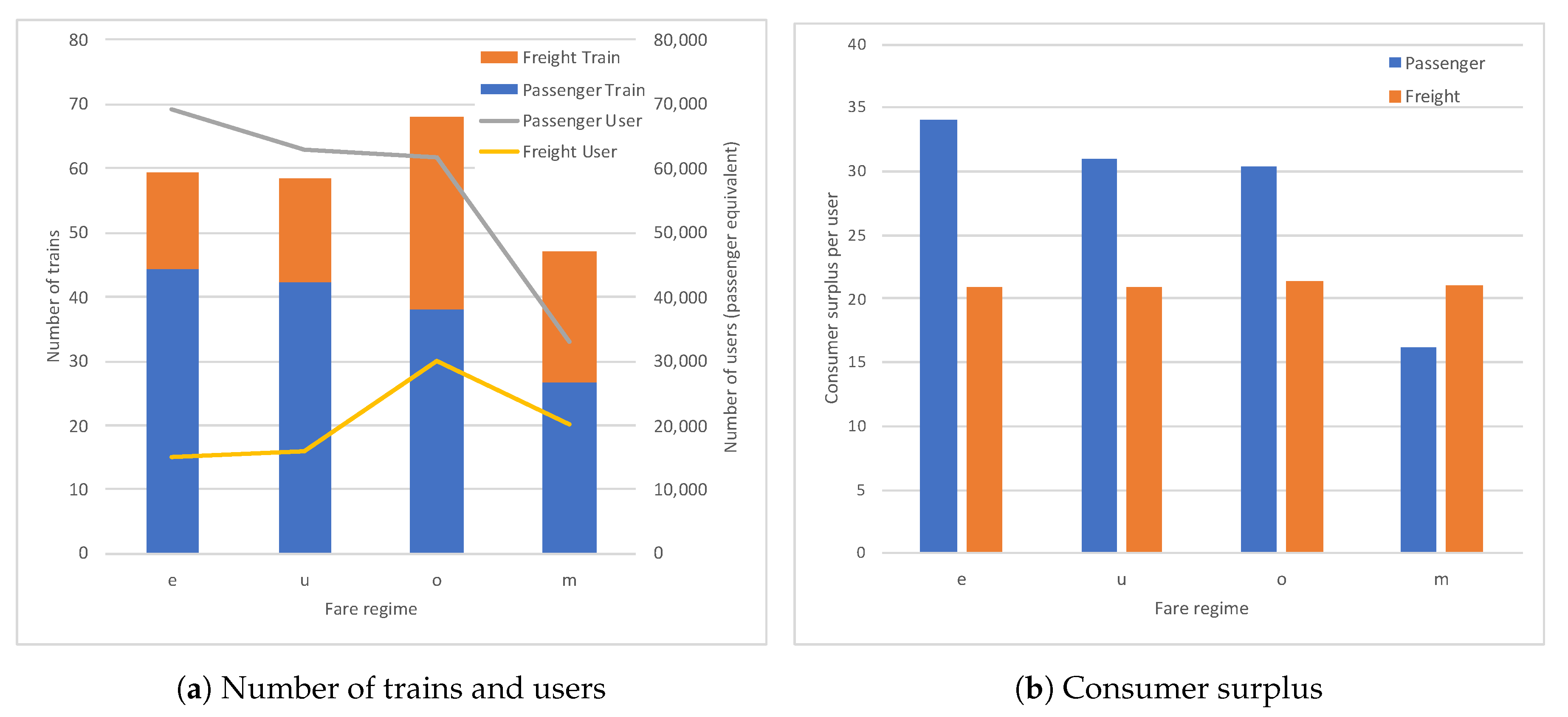
The social optimum utilizes more freight but less passenger trains, which causes the number of passenger trains in the SO the least in regime $e,u$ and o. The ranking of $m_i^{u\ast }$ and $m_i^{o\ast }$ is reversed, compared with the case in which no FOT is allowed where $m_i^{u\ast }<m_i^{o\ast }$. In the example, the time-variant fare removes the queuing cost of freight users, the demand of FOT is boosted to 30.11 trains, and the cost recovery ratio further improved to 1.556. The RHS of Equation (24) then increases in the SO regime, as mentioned in Section 4, the optimal $m_i$ in SO therefore decreases. Figure 4a highlights the number of trains and users among different fare regimes. Two consequences are to be noted due to the decreased $m_i$. First, an earlier $t_0=9.22$, which also contributes to a lower $p^j=12.88$, in addition to the removal of $Q{C}^u$. Note that the changing direction of $t_0$ is again conditional on the schedule delay costs, $p_{N_i}^i$ and $m_i$, similar to the case of the optimal uniform regime. Second, a negative gain per passenger user (−0.088). The consumer surplus of passenger users in the SO ranks the lowest among regimes $e,u$ and o, as shown in Figure 4b. The operator chooses to trade welfare gain from passenger users for that of freight users, as the time-varying fare for freight users generates 0.447 welfare gain per user by eliminating the queuing cost. Recall that in Equation (24), to add or to reduce the number of passenger trains when switching the fare regime from optimal uniform to SO is decided by the sign of $m_{j}s·\partial \overline{{\delta }_j}/\partial m_i-Q{C}_{m_i}^u-R{V}_{m_i}^o$. Given the optimal departure pattern is $FPF$, the sum of the first two terms $m_{j}s·\partial \overline{{\delta }_j}/\partial m_i-Q{C}_{m_i}^u$ is proportional to ${(m_i+m_j)}^2$ in linear MUT specification, and $R{V}_{m_i}^o$ varies with ${m_i}^4$. The number of freight trains $m_j$ is relatively large so that the sign of the three terms turns positive, as in the current example. One may expect that if the freight users have constant-step MUT, where the first two terms vary with proportionally with $m_i+m_j$, it is less likely $m_{j}s·\partial \overline{{\delta }_j}/\partial m_i$ exceeds the sum of $Q{C}_{m_i}^u$ and $R{V}_{m_i}^o$, and the number of passenger trans increases in the SO regime. We verify this expectation in Section 6.4.

As just noted, the trade-off between providing passenger and freight train in the SO regime, to a large extent, is determined by the relative size of demand of the two user groups. By the design of the base case, the initial ratio between the number of passenger and freight trains in the no-fare regime is about 3:1. Ultimately, if the freight demand is small enough, such trade-offs become unnecessary, and the resulting optimal number of passenger train would eventually approach to the case with only passenger service, where the SO regime calls for more passenger trains than the optimal uniform regime. However, our result suggests that the optimal number of passenger trains can be reduced in the SO regime, given reasonable level of freight demand. The passengers are likely to be worse-off in the SO regime than in both no-fare and optimal uniform fare regime, which contradict to conclusion of the case with only passenger service. Considering the freight users have the highest consumer surplus (21.42) in the SO regime, it is clear that an equal rebate of the fare to all passenger and freight users may not necessarily be a Pareto improvement.

6.1.4. Private Profit Maximization

As discussed in Section 5.1, the private operator charges users a monopoly markup decided by the multiplication of the demand sensitivity and the demand level of the respective user group. The results show that the generalized price of passengers and freight users in profit maximization regime is increased to 49.91 and 13.55, respectively, along with a 46% drop in passenger usage and 33% in freight. In contrast to the similar fare levels for the two user groups in the optimal uniform fare regime, the average fare of passenger (37.82) is now about 4 times as high as the freight fare (9.66). The distorted generalized price causes the average consumer surplus of passengers to drop significantly to 16.18, well below that of all the fare regimes by a public operator. By contrast, the average consumer surplus of freight users almost remains unchanged compared with the SO regime. The reason is that lower supply in the number of passenger trains lessens the scheduling cost of freight users, which balances freight users’ loss in consumer surplus. As a result of the lower scheduling cost, the welfare gain from freight users in profit maximization is even higher than in the SO regime, despite of the welfare loss of passengers greatly increases. In the following subsection, we continue to investigate how the welfare loss due to private rail operation can be affected by road pricing.

6.2. Unpriced Road Traffic Congestion

To compare the relative welfare loss by the unpriced road traffic congestion and by the private rail operation, the relative efficiency is recalculated by treating the second-best optimal transit fare as the base scenario, but not the no-fare regime in the last section. Note $o^{\prime }$ and $m^{\prime }$ as the optimal and profit maximization transit fare regimes when the road is not tolled. The relative efficiency of regime r is given as $W^r=(S{S}^r-S{S}^{o^{\prime }})/(S{S}^o-S{S}^{o^{\prime }})$. Negative relative efficiency indicates a lower surplus than in the base regime $o^{\prime }$. The negative relative efficiencies in

Table 5. The relative efficiency in different types of market distortion (absolute level of social surplus given in the parentheses).

	Public Rail	Private Rail
No road toll	0 (6,217,436)	−1.18 (6,007,346)
With road toll	1 (6,395,504)	−1.78 (5,900,916)

show that private rail operation generate more welfare loss than the absence of road toll. The sizes of the relative efficiency relate, to a lager extent, with the share of the two modes. As per the design of the base case, the rail transit shares 41 percent of the total passenger and freight demand in the SO regime. Such share is not extreme but enough to show the possibility that the private operation in rail can incur greater deadweight loss than the unpriced road congestion.

In the right column of Table 5, the figure indicates that the welfare loss due to private rail operation also depends on whether the road is efficiently priced. One may expect that the pricing on road corrects part of the distortion from private rail operation, our result, however, suggests that the welfare loss, when the road toll is in place, is larger. One of the reason is that the mode choice equilibrium in our example is a corner solution, where passenger users only use the rail. The deadweight loss from road traffic congestion comprises a smaller share of the total loss of welfare, compared with an interior equilibrium where passengers use both of the modes. Another reason is that the welfare loss also depends on how much the FOT demand decreases when the generalized price increased in the best pricing regime. As the results in Section 6.1.4, the freight service generates higher welfare gain in the private profit maximization than in the SO fare regime, due to the lower supply of passenger trains, which implies that lower freight transit demand can lead to lower social surplus. We continue to analyze this effect in the next subsection.

6.3. Demand Elasticity

The base case in the Section 6.1.3 shows that the operator chooses to supply less number of passenger trains in the SO regime, which is a result of lowered generalized price of freight users. Given the freight demand elasticity depends on various factors, including upper stream transportation mode, parcel type, receivers’ preferences and so on [30], this naturally raises a question of how the demand elasticity of freight users can affect such trade-offs between supplying passenger and freight trains. Given the demand for passenger transit tends to be inelastic [29], we focus the sensitivity analysis on freight demand elasticity. To maintain the usage at the optimal uniform regime in the base case, the parameter $A_{\eta }$ and $B_{\eta }$, $\eta =i,j$ are adjusted with demand elasticity.

The changes of number of trains with freight demand elasticity are presented in Figure 5. As expected, the number of freight trains utilized in the SO regime decreases with the elasticity. This is because the freight users become insensitive to the decrease in generalized price by the removal of queuing cost. With the demand hold fixed in the optimal uniform regime, the gap of the number of freight trains between the SO and the optimal uniform regime gradually decreases. It is less costly to supply a passenger train when the number of freight trains decreases. The number of passenger trains thus slightly increases in the SO regime. In private operation, we find that the number of trains are more sensitive to the price elasticity. Since we maintain the demand at the optimal uniform regime, the increase in markups, which leads to the decrease of number of freight trains, is a straightforward result of increasing in the demand sensitivity parameter $B_j$. It is noteworthy that in the no fare regime the freight users are priced in the same way as in the optimal uniform, and the difference of the number of freight trains between the two fare regimes owes to the efficient pricing of passenger train usage in the optimal uniform regime. As the price elasticity of passengers remains unchanged in the experiment, the difference is not affected when the price elasticity of freight users varies. All in all, we find the total number of trains is higher in the SO regime than in the optimal uniform regime, regardless of the price elasticity of freight demand. The finding is in line with the case for only passenger service, where the optimal time-varying transit fare calls for more trains than the optimal uniform fare. All the changes in consumer surplus increase as the elasticity decreases except for the freight users in the profit maximization fare regime.

Figure 6 shows how the welfare gains vary with freight demand elasticity. The gain from freight users falls and that from passenger users increase when freight demand becomes inelastic. Since less elastic demand means less deadweight loss from queuing in the optimal uniform fare regime, it is less beneficial to implement the social optimal fare. Recall that the gain from passenger SO fare is only a function of $m_i$, and that $m_i$ increases in Figure 5, one could explain the increase of welfare gain from passengers. Given the total gain in regime o slightly decreases and the welfare gain in regime u is otherwise unaffected, the relative efficiency of regime u increases.

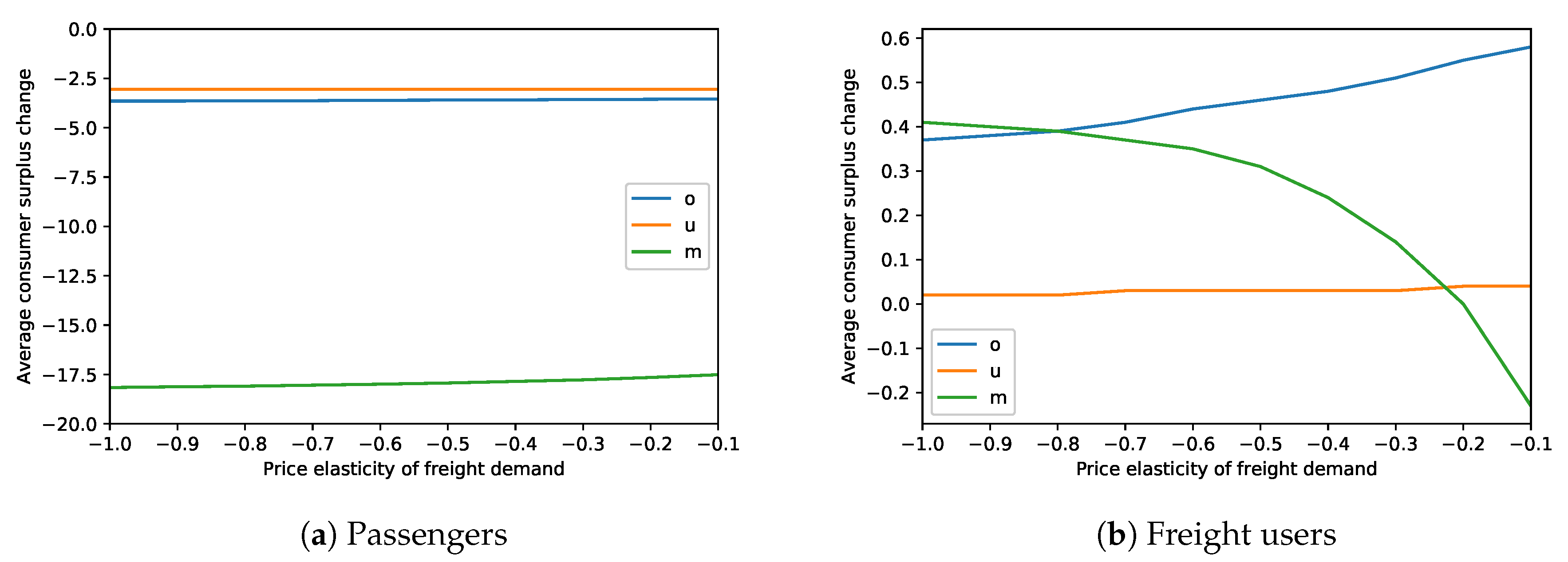
The changes of average consumer surplus compared with the regime e are shown in Figure 7a,b, respectively, for passenger and freight users. All the changes in consumer surplus increase as freight demand becomes less elastic, except for the freight users in profit maximization fare regime. The reason is that the increased consumer surplus of less elastic demand is converted to producer surplus through the monopoly markup $\widehat{\tau }$. Freight users are even worse-off than regime e, as the elasticity drops below −0.2. Such dwindled and even negative change in average consumer surplus of freight users due to the profit maximization fare is indeed accompanied by a mitigated loss in average consumer surplus of passenger users; the absolute change, however, remains negative, compared with the no-fare regime. In the SO regime, the increase of freight users’ consumer surplus change is enlarged as a result of higher willingness to pay. The drop in consumer surplus of passenger users is also slightly increased, though remains negative, because the less elastic freight demand calls for smaller increase of freight trains and then lower marginal cost of adding a passenger train in the SO regime when the queuing cost is removed. It is now clear that our finding from the base case, where passenger transit user is prone to be worse-off in the social optimal fare regime than in the no fare regime, remains valid when the price elasticity of freight demand varies, and when the initial share of freight demand is relatively significant.

Next we expect that the second best FOT fare decreases when freight demand becomes inelastic, as derived by Equation (31). The average revenue per user in the best and the second best optimal time-variant fares are presented in Figure 8, where widened difference can be found between the best and the second best fares, which corresponds to ${\overline{\tau }}_i$ and ${\overline{\tau }}_j$, as the elasticity decreases. A less straightforward result is that the increase in the average revenue per passenger user with the second-best fare, as shown by the line on the top, compared with the lower one for the best SO fare. The reason can be seen by checking the share of freight and passenger trains. If the elasticity hold the same as the base case (−0.33), for example, the ratio between freight and passenger trains is as high as 1.61, compared with about 0.79 in the SO regime of base case. The boosted supply in freight trains entails very high marginal cost of supplying a passenger train, which turns to outweigh the fare reduction due to the second-best fare adjustment $\overline{\tau }$.

Finally, we examine how the welfare loss due to private rail operation is affected by freight demand elasticity. In the last subsection, the result shows that the effective road pricing leads to an lower social surplus than without road pricing in the base case setting of price elasticity. Here we observe the ranking is reversed when the price elasticity of freight demand is relatively high, as shown in Figure 9. As the freight demand becomes elastic, the welfare loss from untolled road increases, and the market power that a private operator can exploit become less, the deadweight loss from road congestion then turns to be a more significant source of loss compared with the private rail operation. Therefore, for relatively elastic demand, the private rail operation with an untolled road tends to generates more welfare loss than that with a tolled road.

6.4. Scheduling Preferences

To illustrating the effect of scheduling preferences regarding welfare gain and optimal service, we consider four types of heterogeneity, linear MUT, constant-step MUT and two mixed cases. For passengers, the parameters of constant-step MUTs for passengers are: $\alpha =8.87$, $\beta =7.45$, $\gamma =11.33$. The MUT parameters for freight users are again set to 20 percent of passengers’. The Parameters of linear MUTs for both types of user are set as the same as the base case. Since the total scheduling cost of each type of user varies with their respective specifications of scheduling preferences, parameter $A_{\eta }$ and $B_{\eta }$ are again calibrated by maintaining the demand in the optimal uniform fare regime, so that all the four cases have the same price elasticities −0.33 in the regime u. The welfare gains and the optimal number of trains in regime o and u are presented in

Table 6. The welfare gains and the optimal numbers of trains in various types of scheduling preferences.

	${\mathit{G}}^{\mathit{oe}}$	${\mathit{G}}_{\mathit{i}}^{\mathit{oe}}/\mathit{User}$	${\mathit{G}}_{\mathit{j}}^{\mathit{oe}}/\mathit{User}$	${\mathit{m}}_{\mathit{i}}^{\mathit{o}}$	${\mathit{m}}_{\mathit{j}}^{\mathit{o}}$	${\mathit{m}}_{\mathit{i}}^{\mathit{u}}$	${\mathit{m}}_{\mathit{j}}^{\mathit{u}}$
Linear-Linear	67,692	−0.089	0.448	37.96	30.15	42.41	16.00
Step-Step	362,054	4.797	0.827	15.72	54.35	12.06	50.63
Linear-Step	111,213	1.981	−0.068	54.40	96.15	43.38	63.87
Step-Linear	193,532	3.694	0.054	16.52	39.03	23.56	22.18

.

In Section 6.1.3, we anticipate that if the freight user have constant-step MUT, the number of passenger trains in the SO regime may not be less than the optimal uniform regime. Our experiment here indeed shows expected result. In the combinations of scheduling “Step-Step” and “Linear-Step”, where freight users have constant-step MUT, the optimal number of passenger trains in the SO regime increases, i.e., $m_j^o>m_j^u$. This is because that the average schedule delay cost of freight users varies more slowly with the number of trains than with linear MUT, the operator does not have to trade the number of passenger trains for that of freight trains any more. Consequently, the average gain per passenger, which is negative in the base case due to the trade-off between the two types of trains, now turns to positive in the two combinations where freight users have constant-step MUT. It is also noteworthy that as result of removing deadweight loss from both passenger and freight users, the total number of trains in the SO regime is larger than the optimal uniform regime in all the combinations of preferences. Another finding is that if either user group has constant-step MUT, the total welfare gain is higher than the case where both groups have linear MUTs. This is in line with the intuition that the users with constant-step MUT tend to have a more concentrated departure pattern in the no-fare regime, it is then more gainful to redistribute the passengers and the freight users to less congested departure times by reducing the crowding cost of passengers and the queuing cost of freight users, respectively.

7. Conclusions

We have analyzed the passenger and freight transit users’ scheduling behavior and their interaction with operator’s fare regimes. Users’ departure time choices are depicted by a transit crowding model for passenger and a deterministic bottleneck model for freight users, respectively.

Under plausible assumptions, we find that the time-varying social optimal fare can make passenger users worse off, but freight users better off, which suggests the fare rebate should not be equal in order to achieve Pareto improvement. The social optimal time-varying fare also calls for more trains than other inefficient fare regimes. The finding is in line with the conclusion when only passenger service is provided, but is contradictory to the conventional understanding gained from road traffic where capacity investments and efficient pricing are substitutes for mitigating congestion. In particular, we find that the number of passenger trains can be reduced in the social optimal fare regime to allow more freight trains, if freight demand is large enough or if freight users have linear MUT preferences.

We show that the congestion toll on an alternative road plays an important role in deciding transit fare. A public transit operator has to adjust the fare level to a lower level in order to compensate the uninternalized congestion on the road. While for a private operator, the loss from monopoly markup is related with whether road pricing is in place. If the freight demand is relatively inelastic, the implementation of road toll can lead to further loss of welfare in private rail operation. Such effect should be considered in transit fare policy assessment.

Our findings are subject to several caveats, which require future work to validate if they are directly applicable in practice. First, in this paper we assume that the number of departure intervals in the optimal timetable is limited. For each service type, only single continuous service window is allowed between another type of service. However, the optimal timetable of track sharing services depends on how many number of freight service windows are allowed in a timetable of passenger trains. The degree of heterogeneity in scheduling preferences of users would actually affect the optimal number of departure intervals. It can be anticipated that low degree of heterogeneity tends to have less separated departure times, then the number of departure intervals in the optimal timetable would increase. In such cases, it is possible that with our single service window assumption the operating cost and the welfare gain of fare regimes are overestimated. We generally did not consider the case when the assumption of single service window is lifted, but we do conduct an experiment in which the optimal timetable problem is modeled as an mixed integer non-linear programming (MINLP), as discussed by Carey et al. [8] and Behiri et al. [11]. While the result shows that the single service window is still the optimal departure pattern when the parameters of scheduling preferences slightly violate the condition of proposition A1, it is in no sense collectively exhaustive. Without the assumption of single service window, a problem specific MINLP solving algorithm is complex, as indicated by Caprara et al. [9] and Cacchiani and Toth [10]. To include the trip-timing choice of users in the model would make the computation of the optimal timetable and the number of trains more difficult. It would be more appropriate to be investigated in a separate study.

Second, our numerical analysis is solely based on synthetic data. On one hand, we assume passenger crowding cost to be linear. Despite the fact that several estimates from European countries [31,32] support this assumption, the crowding cost function ultimately become very steep when the density of passenger approaches the physical limit. Empirical study from Japanese survey data [27] shows that the crowding cost function is approximately quadratic. As the shape of crowding cost function affects welfare gain of passenger fare [16], it is natural to extend the discussion of welfare distributional effect between passenger and freight users to other shapes of crowding cost function. On the other hand, the magnitude of these estimates can affect the optimal number of passenger and freight trains for the respective type of service, although the general requirement of more trains in the social optimal fare regime does not like to change. More robust conclusions rely on the precise estimation of user preferences. Future works that obtain such estimates require specific care in the survey design where the FOT service is provided, and would validate the robustness of our current conclusion.

Third, we assume that the operating cost is a linear function of number of trains and that the capacity per train is fixed. As indicated by Kraus and Yoshida [14], variable train capacity leads to variable operating cost per train. The capacity cost per train can also be a linear function, compared with a constant in our assumption. Given the fact that increasing the capacity of existing trains can be more convenient for users than an additional train, extensions that allow variable train capacity adds another dimension to the long run optimal service problem. It would provide further insight on the optimal fleet capacity in different fare regimes, and permit consideration of self-financing transit capacity with track sharing freight service provided, as the analysis by de Palma et al. [16] for passenger service.

Fourth, scheduling and crowding preferences are assumed to be homogeneous within user group. If we allow passengers and freight users to differ their scheduling and crowding preferences, the current solution of mode choice equilibrium would change, and may result in equity implications different from our current findings. In addition, with heterogeneous users, it is more likely that the time window for the daily maintenance of the rail transit operator is affected. This adds the scheduling preference of the operator, which is different from the users’, to the optimal timetable problem. It also brings more challenges to future work that develops comprehensive MINLP solving algorithms.

Finally, we have considered deterministic travel time, and the service reliability of both modes is ignored. Since rail transit and road generally provide different levels of service reliability, the mode choice behavior of the user can be affected if their valuation of travel time is reliability heterogeneous, and the effect of reliability become significant in large networks. To incorporate the effect of service reliability in the model is not a simple extension of the current analysis, and would require particular attention in the trade-offs between tractability and realism.

References

- Visser, J.; Nemoto, T.; Browne, M. Home Delivery and the Impacts on Urban Freight Transport: A Review. Procedia Soci. Behav. Sci. 2014, 125, 15–27. [Google Scholar] [CrossRef] [Green Version]
- Holguín-Veras, J.; Wang, C.; Browne, M.; Hodge, S.D.; Wojtowicz, J. The New York City Off-hour Delivery Project: Lessons for City Logistics. Procedia Soci. Behav. Sci. 2014, 125, 36–48. [Google Scholar] [CrossRef] [Green Version]
- Diziain, D.; Taniguchi, E.; Dablanc, L. Urban Logistics by Rail and Waterways in France and Japan. Procedia Soci. Behav. Sci. 2014, 125, 159–170. [Google Scholar] [CrossRef] [Green Version]
- Cochrane, K.; Saxe, S.; Roorda, M.J.; Shalaby, A. Moving freight on public transit: Best practices, challenges, and opportunities. Int. J. Sustain. Transp. 2017, 11, 120–132. [Google Scholar] [CrossRef]
- Kikuta, J.; Ito, T.; Tomiyama, I.; Yamamoto, S.; Yamada, T. New Subway-Integrated City Logistics Szystem. Procedia Soci. Behav. Sci. 2012, 39, 476–489. [Google Scholar] [CrossRef] [Green Version]
- Fatnassi, E.; Chaouachi, J.; Klibi, W. Planning and operating a shared goods and passengers on-demand rapid transit system for sustainable city-logistics. Transp. Res. Part B Methodol. 2015, 81, 440–460. [Google Scholar] [CrossRef]
- de Palma, A.; Lindsey, R. Optimal timetables for public transportation. Transp. Res. Part B Methodol. 2001, 35, 789–813. [Google Scholar] [CrossRef]
- Carey, M.; Lockwood, D. A Model, Algorithms and Strategy for Train Pathing. J. Oper. Res. Soc. 1995, 46, 988–1005. [Google Scholar] [CrossRef]
- Caprara, A.; Fischetti, M.; Toth, P. Modeling and Solving the Train Timetabling Problem. Oper. Res. 2002, 50, 851–861. [Google Scholar] [CrossRef]
- Cacchiani, V.; Toth, P. Nominal and robust train timetabling problems. Eur. J. Oper. Res. 2012, 219, 727–737. [Google Scholar] [CrossRef]
- Behiri, W.; Belmokhtar-Berraf, S.; Chu, C. Urban freight transport using passenger rail network: Scientific issues and quantitative analysis. Transp. Res. Part E Logist. Transp. Rev. 2018, 115, 227–245. [Google Scholar] [CrossRef]
- Robenek, T.; Azadeh, S.S.; Maknoon, Y.; de Lapparent, M.; Bierlaire, M. Train timetable design under elastic passenger demand. Transp. Res. Part B Methodol. 2018, 111, 19–38. [Google Scholar] [CrossRef] [Green Version]
- Vickrey, W.S. Congestion theory and transport investment. Am. Econ. Rev. 1969, 59, 251–260. [Google Scholar] [CrossRef]
- Kraus, M.; Yoshida, Y. The Commuter’s Time-of-Use Decision and Optimal Pricing and Service in Urban Mass Transit. J. Urban Econ. 2002, 51, 170–195. [Google Scholar] [CrossRef]
- Tian, Q.; Huang, H.J.; Yang, H. Equilibrium properties of the morning peak-period commuting in a many-to-one mass transit system. Transp. Res. Part B Methodol. 2007, 41, 616–631. [Google Scholar] [CrossRef]
- de Palma, A.; Lindsey, R.; Monchambert, G. The economics of crowding in rail transit. J. Urban Econ. 2017, 101, 106–122. [Google Scholar] [CrossRef]
- Arnott, R.; de Palma, A.; Lindsey, R. Economics of a bottleneck. J. Urban Econ. 1990, 27, 111–130. [Google Scholar] [CrossRef]
- Vickrey, W. Pricing, metering, and efficiently using urban transportation facilities. In Proceedings of the 52nd Annual Meeting of the Highway Research Board, Washington, DC, USA, 22–26 January 1973; pp. 36–48. [Google Scholar]
- Tseng, Y.Y.; Verhoef, E.T. Value of time by time of day: A stated-preference study. Transp. Res. Part B Methodol. 2008, 42, 607–618. [Google Scholar] [CrossRef] [Green Version]
- Kuo, A.; Miller-Hooks, E.; Mahmassani, H.S. Freight train scheduling with elastic demand. Transp. Res. Part E Logist. Transp. Rev. 2010, 46, 1057–1070. [Google Scholar] [CrossRef]
- Knockaert, J.; Verhoef, E.T.; Rouwendal, J. Bottleneck congestion: Differentiating the coarse charge. Transp. Res. Part B Methodol. 2016, 83, 59–73. [Google Scholar] [CrossRef] [Green Version]
- Taniguchi, E.; Thompson, R.G. Modeling city logistics. Transp. Res. Rec. J. Transp. Res. Board 2002, 1790, 45–51. [Google Scholar] [CrossRef]
- Niels, T.; Hof, M.T.; Bogenberger, K. Design and Operation of an Urban Electric Courier Cargo Bike System. In Proceedings of the 2018 21st International Conference on Intelligent Transportation Systems (ITSC), Maui, HI, USA, 4–7 November 2018; pp. 2531–2537. [Google Scholar] [CrossRef]
- Schocke, K.O.; Höhl, S.; Quitta, A.; Schäfer, P. Commercial traffic 2.0—analysis and recommendations of delivery strategies for the package delivery industry in urban areas. In Urban Freight Transportation Systems; Elsevier: Amsterdam, The Netherlands, 2020; pp. 79–100. [Google Scholar] [CrossRef]
- Cherrett, T.; Dickinson, J.; McLeod, F.; Sit, J.; Bailey, G.; Whittle, G. Logistics impacts of student online shopping—Evaluating delivery consolidation to halls of residence. Transp. Res. Part C Emerg. Technol. 2017, 78, 111–128. [Google Scholar] [CrossRef] [Green Version]
- Hjorth, K.; Börjesson, M.; Engelson, L.; Fosgerau, M. Estimating exponential scheduling preferences. Transp. Res. Part B Methodol. 2015, 81 Pt 1, 230–251. [Google Scholar] [CrossRef] [Green Version]
- Xie, C.; Fukuda, D. Scheduling Preference Modeling of Rail Passengers in the Tokyo Metropolitan Area and Evaluation of Time-Varying Fare Policy for a Congested Urban Railway Line. J. Jpn. Soc. Civil Eng. Ser. D3 2014, 70, I_535–I_548. [Google Scholar] [CrossRef] [Green Version]
- Kato, H. Value of Travel Time: Theory and Practice; Gihodo Shuppan: Tokyo, Japan, 2013. [Google Scholar]
- Oum, T.H.; Waters, W., II; Fu, X. Transport Demand Elasticities. In Handbook of Transport Modelling; Hensher, D.A., Button, K.J., Eds.; Emerald Group Publishing Limited: West Yorkshire, UK, 2007; Volume 1, pp. 239–255. [Google Scholar] [CrossRef]
- Beuthe, M.; Jourquin, B.; Urbain, N. Estimating Freight Transport Price Elasticity in Multi-mode Studies: A Review and Additional Results from a Multimodal Network Model. Transp. Rev. 2014, 34, 626–644. [Google Scholar] [CrossRef]
- Whelan, G.; Crockett, J. An investigation of the willingness to pay to reduce rail overcrowding. In Proceedings of the First International Conference on Choice Modelling, Harrogate, UK, 30 March–1 April 2009; Volume 30. [Google Scholar]
- Wardman, M.; Whelan, G. Twenty years of rail crowding valuation studies: Evidence and lessons from British experience. Transp. Rev. 2011, 31, 379–398. [Google Scholar] [CrossRef]
Figure 1.
A single track rail transit with passenger and freight service.
Figure 2.
Graphical solution to utility maximization by departure time choice.
Figure 3.
Graphical solution to optimal timetable by service switching time .
Figure 4.
Comparison of main figures between fare regimes: Base-case, FOT allowed.
Figure 5.
Influence of the price elasticity of freight demand on the optimal number of trains.
Figure 6.
Influence of the price elasticity of freight demand on welfare gain.
Figure 7.
Average consumer surplus change.
Figure 8.
Best and second-best transit fares.
Figure 9.
Welfare loss from private rail operation with and without road toll.