Towards Sustainable Urban Spatial Structure: Does Decentralization Reduce Commuting Times?

1
Housing Urban Finance Institute, Korea Housing & Urban Guarantee Corporation (HUG), BIFC, 40 Munhyeon-geumyung-ro, Nam-gu, Busan 48400, Korea
2
Department of Public Administration, Kangwon National University, 1, Gangwondaehak-gil, Chuncheon-si, Gangwon-do 24341, Korea
*
Author to whom correspondence should be addressed.
Sustainability 2019, 11(4), 1012; https://0-doi-org.brum.beds.ac.uk/10.3390/su11041012
Submission received: 31 December 2018
/
Revised: 6 February 2019
/
Accepted: 7 February 2019
/
Published: 15 February 2019
(This article belongs to the Special Issue Spatial Analysis of Urbanization towards Urban Sustainability)
Abstract
:This paper contributes to the existing debate on the co-location hypothesis, by devising a proximity measure and controlling for a set of other urban form measures. Utilizing the LEHD (Longitudinal Employer–Household Dynamics) Origin-Destination Employment Statistics (LODES) data that provide the number of jobs by a finer geography, this paper measured the degree of centralization, proximity, and job–housing mismatch. Multiple regression analysis revealed that the job–worker proximity leads to a shorter commuting time. In addition, the results focusing on suburban areas revealed that the impact of the job–worker imbalance and the impact of job–worker mismatch on the commuting time are greater in the suburb in comparison with the city center.
1. Introduction
The evolution of spatial structure plays a significant role in shaping interactions among decision-making agents in cities. The development of transportation technologies transformed old port city centers and connected inland areas to each other. As the railway system came into existence, firms that had been locked in the port center could move along the rail lines. Around 1910, trucks appeared, and the network of roads made it possible for firms to move goods to further inland locations at lower shipping costs. Residential suburbanization was in line with the relocation of firms because workers wanted to locate close to their employers. The flattening of the density gradients for firms and residences continued to gain momentum as retailers and office employment decentralized. Most urban economists view the spatial transformation from monocentric to polycentric structures as an adjustment process that mitigates negative externalities, whereas many urban planners blame excessive decentralization and sprawl for more congestion and longer commuting distances.
The modern theory of urban spatial structure was developed by Alonso [1], Muth [2] and Mills [3], in order to explain the residential location pattern in a monocentric city, where people commute to work to the city center. The critical element of the theory is the spatial (no) arbitrage condition: there are no economic rents to be extracted from switching locations within a city. In detail, the theory argues that (1) the marginal rate of substitution between land consumption and other goods equals the rental price of land, and (2) the land rent reflects a trade-off between land consumption and transportation cost. In a monocentric city, where employment is concentrated on a single point of the city and all residents commute to the center point, the residential density decreases with the distance from the center, because (1) the rental price of land decreases with the distance from the center, and (2) thus as the distance from the city center increases, there is a decrease in the capital–land ratio in housing production (Mills [3] and Kraus [4]).
While it serves as the cornerstone for understanding the economics of cities, the early theory of monocentric cities has two critical limitations. The standard consumer utility maximization problem and its dual problem of the aggregate land value maximization assume that the transportation cost is exogenously given. If we introduce congestion externalities into our monocentric city model, the location of residences may influence the commuting cost (Wheaton [5]). In this setting, the travel cost becomes endogenous, and accordingly, the travel cost and residential density must be determined simultaneously. This land-use–transportation interaction model was suggested by Mills [3] and Solow [6]. Wheaton [5,7] presented a model on how the market equilibrium and socially optimal density differ in a monocentric city when the congestion externalities exist.
By contrast, the multicenter equilibrium configuration hypothesis is empirically supported by Timothy and Wheaton [8] from the worker’s perspective. Timothy and Wheaton, using the U.S. Census’ Public Use Micro Sample (PUMS) data, estimated an earnings equation by place of work (PWPUMA), controlling for other variables that might influence the worker’s payroll—the demographic and occupational characteristics of the workers. They found that wages varied from 15% to 20% between places of work, and the average wage was higher in work places located in the center of metropolitan areas. Glaeser and Kahn [9] provided similar evidence using ZIP code data. From the cross-MSA (Metropolitan Statistical Area) comparison between employment and commute gradients, they found that commute times have a weaker link to the distance from the central business district. Similarly, housing prices do not decrease monotonically with the distance.
While a large strand of urban economics literature has investigated the empirical implications between urban spatial structure and commuting behavior, the results are mixed because of the differences in the geographic scales, data sources, methodologies, and specifications of empirical models. The objective of this paper is to answer the question of whether or not the spatial proximity between jobs and workers (put differently, the degree of land-use mix) contributes to shorter commuting. In order to test for the relationship, this paper first creates indexes characterizing urban spatial structure. Then, the paper investigates how well and in which direction the proximity explains workers’ commuting patterns—after controlling for other important dimensions that might affect the commuting time. In addition, this research looks into the job–worker balance and job–worker mismatch by concentric zone (city versus suburb), and investigates the impact of the locational differential on commuting time.
2. Literature on Co-Location between Jobs and Workers
2.1. Co-Location Leads to Shorter Commuting
A large body of literature has tried to understand the impact of spatial structure on commuting patterns. Some of them have discovered that the dispersion results in shorter commuting, and others have argued against the co-location hypothesis. Gordon et al. [10] estimated a regression equation of the mean commuting time on the degree of monocentricity, controlling for the residential, commercial, and industrial density; economic structure; urban size; and income measures at the aggregate, metropolitan level. They concluded that dispersion facilitates shorter commutes. As for the measure of the spatial structure, the authors calculated the degree of monocentricity for each SMSA (Standard Metropolitan Statistical Area) as the proportion of SMSA employment found in its largest city. In a descriptive study, Gordon et al. [11] compared the commuting times between 1980 and 1985 for each metropolitan area, and conjectured that that dispersion results in shorter automobile commuting times. From the paired t-test, they argued that cities, which are thought of as being dispersed, such as Dallas, Phoenix, and San Diego, show shorter automobile commuting times than cities like New York, Chicago, and Baltimore. They did not attempt to measure the degree of polycentricity, and did not test for any causal relationship between spatial structure and commuting.
Levinson and Kumar [12] compared two travel surveys conducted in two different times for the same area, and concluded that the commuting times remained stable or declined over the period of 1968 to 1988, while the average commuting distance increased. Rather than quantifying the spatial structure and testing for the causal relationship between the spatial configuration and commuting, they simply argued that the constancy in trip duration would (indirectly) support a feedback mechanism or a spatial adjustment process between households, firms, and other organizations. Peng [13] also supported the co-location argument, showing that the jobs–housing ratio is negatively associated with vehicle miles traveled (VMT) per capita.
Tsai [14] created indices for both decentralization and subcentering (i.e., local clustering) using the 1990 Census Transportation Planning Package (CTPP) data. As for the measure of population and employment decentralization, Tsai calculated the Gini coefficients for the population and employment densities by taking the traffic analysis zone (TAZ) as the basic spatial unit. In terms of dispersion for population and employment, Moran’s I statistics and the Geary coefficients were used. The bivariate correlation coefficients between those measures and the vehicle miles traveled (VMT) showed mixed results with respect to city size. Tsai found that the correlation between the job-based Moran coefficient and the VMT was positive and significant only for the metropolitan group with a population between 500,000 and 699,000. The population-based Moran index has a significant, negative effect on the VMT at the worker-level regression. This means that subcentering facilitates a reduction in VMT. In addition, the Gini coefficients for the jobs and population did not explain the variation of VMT, meaning that decentralization does not have a significant effect on the commuting distances. One interesting finding of the research, from the multilevel specification, is that the metropolitan-level urban form indices as a whole jointly explain only a small portion of the total individual VMT.
At the worker level, Clark et al. [15] compared the commuting distances and time of the workers who change their work place with those of workers who do not change, and concluded that the workers whose commuting was very long try to locate their residences close to their jobs when they have to relocate. Crane and Chatman [16] tested whether or not job decentralization shortens the average commute distance by using individual-level travel data and metropolitan-level employment data. They clarified that the spatial structure they measured is of employment dispersal, rather than (de)concentration. By classifying counties into “central” and “outlying”, which follows the official U.S. metropolitan area definitions, they could calculate the measures of dispersal for the workers and jobs as the share of total population and total employment in the outlying counties of the metropolitan areas. Those measures can be thought of as the opposite to the measure of monocentricity by Gordon et al. [10].
Crane and Chatman’s study stands out in that they found that the effects show different patterns by industry. It is true that the patterns of decentralization are not the same for different categories of jobs in urban history. Manufacturing jobs, for example, are much more dispersed than commercial banking employment (Glaeser and Kahn [9]). Furthermore, the authors took into account the endogeneity of land rents, wages, employment status, and car access, which the previous literature did not consider. By including the industry-specific employment share variables into the regression, the authors provided an interesting result, namely: employment dispersal for the manufacturing and the government sector is associated with longer commutes. They interpreted this result as evidence that those sectors have experienced clustering rather than decentralization.
Cho et al. [17] tried to understand whether employment subcenters play a role in determining the location of residence at the micro level. The multinomial logit model of the residential location decision showed that workers are more likely to choose their residential locations with greater accessibility to employment subcenters.
2.2. Co-Location Hypothesis Does Not Hold
Cervero [18] presented empirical evidence that rejects the co-location argument. A regression model of the commuting flow and housing supply revealed that the jobs–housing balance is not significantly related to the degree of self-containment. This is because restrictions in housing production and high housing prices hinder workers from living close to their job locations. Similarly, Cervero and Wu [19] concluded that employment decentralization does not contribute to a reduction in commuting distances or to the number of car drivers in the San Francisco Bay area. They conjectured that the increase in commuting with decentralization would come from the lag in housing production due to exclusionary land-use regulations, particularly in the suburban employment centers (Cervero and Wu [20]). Loo and Chow [21] expressed a similar observation; decentralization could be a problem when workers could not find suitable housing adjacent to suburban employment centers.
Similar to the study of Cervero and Wu [19], which considers workers’ job classifications, Levine [22] investigated the impact of suburban employment growth on commuting for different income groups. The study found that the lower level of housing choice hinders low-income households from being matched to job locations, and consequently produces longer commutes. Similarly, Aguiléra [23] found that in the three large metropolitan areas in France, workers living in subcenters do not commute within the subcenters, and thus produce longer commuting distances. In addition, the majority of jobs located in the subcenters are taken by non-residents who commute to those subcenters from distant locations.
Sarzynski et al. [24] used a structural model to test the effect of urban form and congestion. The four endogenous variables are (1) the degree of congestion, (2) network usage, (3) transportation network, and (4) spatial structure indicators. For the 50 large metropolitan areas, the congestion outcomes were measured as (1) the mean travel time to work, (2) the annual average daily traffic per freeway land, and (3) the annual person hours of delay per capita. The indicators for the metropolitan spatial structure include density/continuity, housing–job proximity, job compactness, mixed use, housing centrality, nuclearity, and housing concentration. After controlling for the level of congestion for 1990, the commute time for 2000 was negatively related to the job–housing proximity. However, in the equations for average daily traffic and for delay per capita, the coefficient of density/continuity indicator turn out to be positive.
Sultana and Weber [25] defined sprawl as a process of rapid population growth occurring outside of built-up areas, and showed that workers in sprawling areas commute for longer than those who live in the center in Birmingham and Tuscaloosa, Alabama. This finding could be interpreted as indirect evidence that the co-location mechanism does not necessarily happen in all of the areas in the United States.
Whereas Levinson and Kumar [12] concluded that commuting stays stable over time, the following two studies did not find any evidence for the co-location adjustment process between jobs and residences. Kim [26] concluded that workers who relocate are unlikely to reduce their commuting time and distance. Using panel data for the Seattle Metropolitan region, he suggested that the coordination failure would come from the lagged housing production in fast growing areas. Levinson and Wu [27] delivered an ambiguous result by locale. A descriptive analysis from the 1968, 1998, and 1994 household travel survey data for metropolitan Washington revealed that the larger Washington D.C. region showed little change in commute times, whereas the Twin Cities marked a drastic increase over the decade.
2.3. Polycentricity and Commuting
2.3.1. Debate over ‘Wasteful’ Commuting
The early debate on the polycentric urban form and commuting dates back to the two contradicting arguments raised by Hamilton [28] and White [29]. Hamilton raised the question of whether or not commuting in U.S. metropolitan areas is (in)efficient. Using the 1979 and 1980 Annual Housing Survey data, Hamilton derived the negative exponential density gradients for fourteen United States’ cities. Then, Hamilton calculated the difference between the actual commute and the “required” commute, which is measured as the gap between the distance from the population to the central business district (CBD) and the distance from employment to the CBD. Finally, the paper concluded that 87% of urban commuting is wasteful, and decentralization of employment does not yield any reduction in commuting, even though jobs follow residences.
One of the critical points from the findings is that the monocentric city framework fails to explain the real-world commuting patterns. White argued that Hamilton’s calculation is biased upward, and found that about 11% of all commuting was wasteful. She suggested that wasteful commuting appears to be a minor factor in explaining the commuting patterns of U.S. urban workers by using the 1980 U.S. Census of Population data. Dubin [30] provided a response to Hamilton’s finding that decentralization increases commuting. She set up a model with eight statistical equations and one identity equation to test whether the distance of the actual job from the CBD affects the difference between the current commuting time (distance) and the time (distance). Using the worker-level Baltimore Travel Demand Data, she concluded that mobile individuals commute less as a result of firm decentralization.
This disagreement originated from the different assumptions on the distribution of jobs and houses around the CBD and the selection of spatial units. Hamilton assumed that jobs and houses are uniformly distributed around the CBD, and calculated the population and employment density gradients by taking the average distances from the CBD, which are in line with the classical Alonso–Muth–Mills’ monocentric city configuration. White [29] challenged Hamilton’s approach by proposing that jobs and housing could be differently distributed around the CBD, and workers commute along the existing road network. White divided a metropolitan area into zones, and calculated the commuting distances between each pair of zones, the number of residences in each zone, and the number of jobs in each zone. Using these calculations, White could include the possible circumferential travel patterns as opposed to the Hamilton’s model, in which commuting only occurs along the straight paths emanating from the center location.
A series of related studies were conducted in response to those traffic assignment models. Cropper and Gordon [31] re-examined the “wasteful” commuting argument by adopting White’s notion of irregular spatial distribution of jobs and housing, and by assuming that no household’s utility is lowered when households are reassigned to houses. They used the Baltimore Travel Demand Data, with which they were able to divide the metropolitan area into 498 zones. They concluded that the actual average commute in Baltimore is about five miles, or about half of the average actual commute, which is considerably less than Hamilton’s result. Small and Song [32], by using the 706 traffic analysis zone data for the Los Angeles–Long Beach metropolitan statistical area, calculated the ratio of the actual average commute to the minimum average commute. They observed some degree of excess commuting, which was 33% of the actual commuting time. This result was derived when they considered large jurisdictions as the basic unit of the assignment problem. The percentage rose to 66 when smaller zones were used. Their findings suggest that the difference between the market and optimal solution could depend upon the number of zones used in the assignment model. As the number of spatial units increases (or as the unit zone becomes smaller), we may observe more excess commuting, because when the length of average commute within a small zone is relatively shorter than that between the zones, commuting within the zones is treated as efficient in the assignment model.
2.3.2. Simultaneity between Job–Worker Proximity and Commuting
Fujita and Ogawa [33] presented a theoretical model of multicentric spatial configuration that encompasses the complete simultaneous determination of workers’ and firms’ location patterns, land rents and wage gradients, commuting, and the utility level of households. They concluded that spatial configuration could undergo some degree of “catastrophic” structure change, as opposed to the clear-cut, exclusive land-use segregation between jobs and residences. Henderson and Mitra [34] presented a model of how an imaginary entrepreneur (or developer) develops his or her edge city to maximize profits. Their critical theoretical prediction is surprisingly similar to the Fujita and Ogawa’s. The edge city’s optimizing choice of location, in theory, exhibits a “zig-zag” or “chaotic” pattern over space. Those theoretical insights on the “fuzziness” of the land-use pattern are reaffirmed by Wheaton [35]. In Wheaton’s model, the market equilibrium can lead to a full dispersal if the land use allocation is based on the relative magnitude of the rent levels for each use, rather than deterministically on the highest rent. This argument is based on the assumption that land is allocated by the process of an idiosyncratic or a fuzzy land use competition.
The result of the transition of the land-use pattern is the worker’s spatial equilibrium between the old center city and the suburban employment districts. In order for a worker who commutes a longer distance from the edge to the central business district to reduce his or her commuting cost, the worker has an incentive to relocate to suburban areas and to accept the lower wage. Consequently, the wage differential between different job locations reflects the variation in the average commuting costs, ceteris paribus. Firms also have the strong incentive to decentralize, because they can reduce the most important costs of production, which are land rents and wage. Therefore, we have the compensating equilibrium between work locations within a polycentric metropolitan area; bigger centers (all else equal) have to have longer commuting distances (or, lower commuting speed), higher land rents, and higher wages. White [36] corroborated this indifference premise from the theoretical point of view. If the co-location of jobs and residences becomes possible, we might observe a variety of worker’s wage offer curves, and correspondingly, different types of households’ rent offer curves, depending on the workers’ job locations.
In U.S. cities, employment turns out to be almost as dispersed as residences, and thus land use can be mixed. As metropolitan areas have become multicentered, the employment and residential gradients have been flattened throughout the city. When workers and firms are perfectly matched in location, the problem of traffic congestion would be erased. Critical questions arise in regard to the polycentric urban form, namely: Can this city system be efficient? How do land markets for residential and commercial use work? We noticed that travel demand arises because we assume that jobs are more centralized than households. In the monocentric model, all households travel to the CBD. Then, towards the center, less and less households will travel. In the inward-out commuting polycentric city model developed by Wheaton [35], scale economies (i.e., agglomeration effects in production) play an important role, and thus a completely dispersed city cannot be optimal. In the competitive private market, land will be assigned to the highest bidder. The rent gradients for households and firms, as well as the wage gradient, exist in the private market. Then, a market model can lead to a full dispersal if the land-use allocation is based on the relative magnitude of the rent levels for each use. Therefore, at the extreme case, fully dispersed employment can happen even if some form of agglomeration exists. These cities with no congestion, via the perfect match between residences and firms in location, however, would lose the advantage of productivity. Anas and Kim [37] similarly argue that “when scale economies in shopping are strong relative to the cost of traffic congestion, dispersion becomes unstable.” Therefore, in this problem of an aggregate net value of urban output maximization, the solution of land-use allocation is a partial dispersal. Numerical simulations by Wheaton reveal that, in a mixed land-use city where the productivity declines by a quarter, the employment border moves out. In addition, the percentage of land occupied by firms decreases to an average of 40% in the situation where the proximity between commercial and residential land uses occurs when firms and households compete for the land. They consequently jointly occupy a fraction of the land at any location within a metropolitan area.
There are positive and negative relationships between the transportation cost and the level of centralization in the polycentric equilibrium. Furthermore, if land rents for different uses follow a random process, a fully dispersed employment equilibrium is, in theory, possible. In the private equilibrium, the role of agglomeration is to offset travel costs. However, as an “optimal” city maximizes the aggregate net value of the output, there should be some degree of land-use mix, because the city can benefit from the agglomeration effect. Therefore, there is a complex simultaneity among the proximity between jobs and workers, travel cost, and transportation demand. Travel cost determines wages, travel cost is a function of travel demand, travel demand depends upon land use, land use is a function of rents, and rents are determined by travel cost. Also, a polycentric equilibrium exists with the agglomeration effect.
Empirical works for the identification of the causal relationship from the job–worker proximity (i.e., land-use mixing) to the degree of polycentricity are rare, particularly at the metropolitan level. The early work by Gordon et al. [10] tried to address the influence of the urban spatial structure on travel time. Their measure for the spatial structure was rough, gauging the proportion of the largest city’s employment to the metropolitan area’s total employment. What is more problematic is that the paper took the spatial structure as exogenous.
More relevant research by Lee [38] tested the impact of several urban spatial variables on the commuting time. The research took some variables to instrument the urban spatial structure, namely: metropolitan age, the percentage of core city population, the number of cities with large population, and the industrial structure. However, the research does not provide any justification as to why those instruments, in theory, are linked to the commuting behavior. Old cities tend to be more centralized and have a greater influence of the central city, which could result in longer commuting. Also, we know that manufacturing jobs are more dispersed than the FIRE (finance, insurance, and real estate) sector counterparts. Therefore, jobs for a higher level of services could draw workers from locations far from the city center. The research disregarded the possibility of the systematic variations of commuting time with respect to the industrial composition in space.
The regression results from Lee’s work also seem problematic. The polycentricity variable is not statistically significant in both the OLS (Ordinary Least Squares) and 2SLS (Two-Stage Least Squares) equations in the two different specifications [38]. The result, in part, seems to be originated from the poor measure of polycentricity. The research did not measure the polycentricity directly, but took the ratio of the subcenters’ employment to the sum of the CBD’s and subcenters’ employment. On the contrary, looking at only the distribution of job centers, the index of spatial structure in this research reflects the weighted sum of the jobs-to-workers distances at every location, with the modification of a spatial unit of analysis (which is a floating catchment area.). The measurements of spatial structure are discussed in the following section.
3. Quantifying Urban Spatial Structure
3.1. Data
LEHD (Longitudinal Employer–Household Dynamics) Origin–Destination Employment Statistics (LODES) is the main data source for measuring how local access (i.e., the jobs-to-workers ratio for the inner locations of cities) is centralized towards the city center. This paper uses the latest version of the LODES data (version 7.0). The number of jobs and the number of resident workers have been enumerated onto the 2010 census blocks. The Public Use Micro Area (PUMA) definition still follows the 2000 version. Therefore, in order to obtain the 2010 blocks in line with the 1999 metropolitan area definition, this research created a crosswalk definition file. It relates the 1999 metropolitan areas with the 2010 census blocks, by using the clipping tool in the ESRI ArcGIS software.
3.2. Defining City Center Locations
The base locations for selecting the job center locations for each metropolitan area come from the 1982 Census of Retail Trade. The significant job centers are given as some 1980 census tracts. This research starts with the definition file that contains the longitude and latitude coordinates of the tracts. In order to choose one CBD for each metropolitan area, the 1982 CBD locations layer was mapped onto the layers of (1) the 2010 census tracts, (2) the primary cities of metropolitan areas, and (3) the 1999 metropolitan areas. There are three cases of the pattern of the 1982 CBD locations. First, if only one 1982 coordinate is identified in each metropolitan area, the coordinate is chosen as the CBD location.
Second, if there are two or more 1982 locations that are identified in the primary city of the metropolitan area, the centroid of the 2010 tract is chosen, which has the largest number of jobs. Also, there are cases where multiple 1982 CBD locations fall in the one 2010 tract. Then, the 2010 tract’s centroid is chosen. Finally, if there are no 1982 CBD locations in a metropolitan area, the 2010 tract is chosen that has the largest number of jobs in the primary city of the metropolitan area. The primary city is the one located in the metropolitan area that appears first in the 1999 MSA/CMSA (Combined Metropolitan Statistical Area) name.
3.3. Floating Jobs-to-Workers Ratio
For each location or zone in the metropolitan area, the jobs-to-workers ratio within radius is defined. This buffered area is called the floating catchment area. The choice of is arbitrary with respect to the metropolitan area conditions and other policy perspectives. Peng [13] chose five miles from the traffic analysis zone (TAZ), and Immergluck [39] adopted a two-mile radius at the TAZ level, which was consistent with the neighborhood economic development policies at the time of research. Yang and Ferreira [40] defined the catchment area in the following two ways: (1) areas composed of the 10 closest tracts, and (2) nearby tracts whose centroids are within 10 kilometers of the target tract. Recently, Kneebone and Holmes [41] considered the average commute distance in each metropolitan area as the radius of proximity. This paper used the two-mile as the radius of local access.
The spatial unit of analysis is a census block group, not a block. There are three reasons for aggregating the data to the block-group level. First, at the very local level, a common neighborhood geography is thought to be a block group [42]. Second, because the two-mile radius is short relative to the average commute distance, there are a significant amount of locations that have no resident workers at the block level, which makes the calculation of the local access invalid.
3.4. Centralization of Jobs-to-Workers Ratio (CJW)
After obtaining the jobs-to-workers ratio for every block group, the cumulative percentage of the ratios can be plotted against the cumulative percentage of the sorted distances from the CBD, which yields the centralization index by each metropolitan area. The line is the Lorenz curve. Then, the measure of centrality (CJW) is the area under the Lorenz curve, which can be approximated to the sum of all the trapezoids divided by 2, as follows:
where and are the cumulative percentages of the local access and the distance from the CBD to the location (in fractions), respectively, and is the number of block groups in a metropolitan area. This centralization index measures the degree of job richness at every inner location in a city, with respect to the centrality of the city. A higher centralization means that local jobs (relative to workers) are more concentrated towards the city center.
3.5. Proximity between Jobs and Workers (PJW)
The centralization index measures the degree of centrality of local access at the metropolitan level. The shortcoming of this index is that it does not evaluate the distances between all pairs of locations. The centralization index shrinks the two-dimensional locational patterns into the one dimension, that is, the linear relationship between the center and the edge locations. A multicentric model developed by Wheaton [35] also takes this linearity assumption, that commuting occurs in and out of the city center. This framework alone does not fully explain the current city structure. Urban agglomeration and the forces of the jobs-to-workers proximity have been well documented in the urban economics literature [43]. Partitioning typologies of the structure of cities into both centrality and proximity will provide a more complete picture of the spatial configuration of cities. The proximity index is a simple application to the segregation measures proposed by White [44]. This index measures the average proximity between jobs and workers, and can be interpreted as the overall degree of spatial clustering and concentration between jobs and workers, as follows:
where is the distance from location to , is the total number of jobs, and is the total number of workers. Note that does not always equal , because some portion of workers commute outside of the metropolitan area.
3.6. Density-Based Co-Location Index (BPJW)
3.6.1. Kernel Density Estimation between High Peaks of Jobs and Workers
Duranton and Overman [45] devised a rigorous continuous measure of employment concentration by utilizing the establishment-level data per industry for the entire United Kingdom. The authors calculated the Euclidean distances between every pair of establishments, and estimated the Gaussian kernel smoothing density of the bilateral distances. To that end, their metric is different from the employment density gradient approaches, and does not address any centrality of the spatial structure. As for judging the significance of the candidate local peaks, Duranton and Overman [45], and Redfearn [46], used a type of bootstrapping technique, while McMillen [47] added the second- stage semiparametric regression. This research follows Duranton and Overman’s approach to describe the co-location pattern between extreme values of jobs and extreme values of the resident workers at the block level. For simplicity, this study takes the jobs and workers that are above the 99th percentiles as the high peaks. More rigorous statistical techniques exist, which are designed to detect relative outliers, but using the above-99th percentile cut-off is more straightforward, and the results are not expected to be significantly different. Moreover, applying the McMillen-type non-parametric methods to detect outliers adds additional significant computation time, which virtually makes the main analysis of this research almost impossible.
Using the centroids of the census blocks for jobs and workers, this study begins by calculating the bilateral Haversine distances between all pairs of jobs and workers. Note that the jobs and workers are above the 99th percentiles. With jobs and workers, there are unique distance pairs. The estimator of the density (“K-density”, hereafter) pairwise distances at any target distance is given as:
where is the distance between job locations and worker locations , is the bandwidth, and is the kernel function. For the bandwidth, this paper uses Silverman’s rule of thumb, which is , where is the standard deviation of the pairwise distances [48]. For the kernel function, the Gaussian kernel is used. Note that the kernel estimates are weighted by , which is the product of the number of jobs in the census block and the number of workers in the census block . Here, the unit of the distances for the kernel function is 100 meters.
The support of the density estimator is bound to , because negative distances do not make any practical sense. However, Equation (3) will produce positive density estimates at some adjacent parts of the left side of 0 (zero) . This means that our empirical densities do not add up to one. Following Duranton and Overman [45], this paper adopts Silverman’s reflection technique [48]. First, this analysis augments the original distances by adding the reflections that are the negative values of the distances, in order to give a data set with twice the original number of distances. Then, this procedure winds up with the following modification to Equation (3):
where for . The formula prevents density estimates around some target distances of the right side nearby 0 (zero) from being under-estimated. We set up the target distances vector that contained 1001 evenly spaced points from to (100 kilometers). The distances between the jobs and residences above 100 kilometers can be interpreted as dispersion, and thus are not factored in the K-density estimation. As for the density estimation algorithm, the pairwise distances are linearly binned to the target distances vector, and the kernel estimates are, at each target distance point, derived from the fast Fourier transformation (FFT). In the typical FFT setting, the number of distances is taken to be a power of 2. Then, the final kernel estimates at each target distance are calculated via interpolation. However, this research specifies as the number of target distances explicitly, which is 1001. This set-up skips the interpolation step and saves computation time.
3.6.2. Constructing Counterfactuals
At this stage, the degree of co-location between jobs and residences needs to be evaluated by comparing the actual spatial pattern, calculated as Equation (4), against the hypothesized distances drawn from possible random locations of the jobs and residences. The observed job and worker locations are randomly assigned to the null space. Next, one pseudo K-density is estimated. This procedure is repeated 2000 times. Then, for each target distance, the bootstrapped points are sorted. The standard 95% bootstrap confidence intervals are obtained by selecting the 50th to 1950th values. Here, the null locations for each metropolitan area refer to the census blocks that are assumed for the above-99th percentile jobs and the workers to be located. This paper considers all of the census blocks of the candidate locations, except for the locations without jobs and workers. Duranton and Overman [45] named this calculation as a local confidence interval.
The issue underlying the local confidence interval is that we can evaluate the colocation with respect to only each target distance . We cannot infer how far jobs and residences are from each other at the whole metropolitan scale. For a remedy to this problem, Duranton and Overman [45] proposed the construction of a global confidence interval. The global confidence interval is a band “such that no more than 95 percent of the estimated density functions have even a single value that lies outside the interval at any of the target distance.” [49]. Mathematically, the upper bound for the global 95% confidence interval is defined as a set of 1001 values, such that , where is the number of simulations. The detailed computation procedure is illustrated in Klier and McMillen [49]. Finally, the colocation index for jobs and residences, , is given as follows:
Note that the co-location index is a function of any target distance. Whereas Duranton and Overman evaluated the up to the median value of the bilateral distances, this paper chooses kilometers, assuming that there could be workers who commute long distance from one edge to the opposite edge in a metropolitan area. For example, the 2006–2010 five-year American Community Survey (ACS) revealed that 2.06% of full-time workers are “mega-commuters” who travel 90 or more minutes and 50 or more miles to work in San Francisco–Oakland–Fremont, CA [50].
3.7. Employment Clusters
All of the three indexes (one centralization index and two between indexes) illustrate the overall spatial patterns of the jobs and workers of the cities. One critical drawback of the indexes is that they do not address the nature of the local clustering of economic activities in space. Employment clusters capture the concentration of employment within metropolitan areas, which significantly affects the distribution of jobs and workers. There are two strands of literature on the subcenter identification methods, namely: the simple “cut-off” value specification and the statistical modeling approaches. This research refines those methods, and applies a simpler percentile cut-off approach in order to identify the employment clusters.
3.7.1. Cut-off Value Approach
The early literature tried to identify high-employment nodes within metropolitan areas by using the absolute magnitude and density cut-off approach. McDonald [51] identified a zone or a contiguous set of zones among the 44 postal zones as a subcenter in the Chicago SMSA, by looking at the total employment densities and employment-to-population ratio. He justified his findings by showing that the identified subcenters have statistically significant impacts on the housing and land price gradients.
Giuliano and Small [52] conducted a similar analysis for the Los Angeles (LA) region. They defined 32 subcenters that met the criteria of 10 employees per acre and 10,000 employees. Then, they classified the identified subcenters into five industry groups using the multivariate cluster analysis with the input variables, such as the share of employment in major sectors, the distance from the LA CBD, and employment density. Small and Song [53] doubled Giuliano and Small’s cut-offs to 20 per acre and 20,000 employment for the 1135 transportation analysis zones. However, they did not provide the rationale as to why this change should be made in analyzing the same Los Angeles region. As for the spatial structure, they explicitly considered the measure of dispersion by calculating the Gini coefficient for employment density, as opposed to the simple description done by McDonald [51]. McMillen and McDonald [54] revisited Chicago and explored the nature of the agglomeration economics. They followed Giuliano and Small’s criteria and found 20 subcenters. In order to find the relationship between employment decentralization and commute distances in the San Francisco Bay area, Cervero and Wu [19] also used the size and density criteria.
Bogart and Ferry [55] used the same density and size approach in Giuliano and Small [52] for the Cleveland area using the Census Transportation Planning Package (CTPP) data, and identified nine subcenters. Anderson and Bogart [56] also took a similar approach, with slight modifications to the Giuliano and Small method. Giuliano et al. [57] adopted the same cut-off approach, and experimented with different cut-offs. Their descriptive analysis revealed that the spatial layout of the LA region remained “stable”, and both concentration and dispersion occurred during the 1980–2000 period.
Gardner and Marlay [58] defined an employment cluster as an area that has a minimum total employment of 50,000. To detect a cluster, they first identified high-employment census tracts. A tract with the ratio of jobs to residents of 1.0 was considered to be of high employment. Then, for each core, adjacent tracts were added to form a cluster if the candidate tracts had at least 1000 jobs per square mile. This process continued building the cluster until all of the nearby tracts met the job density threshold. In addition, the algorithm is designed for employment clusters not to overlap.
From a methodological standpoint, the subcenter identification technique using the threshold density and size criteria has some shortcomings, while the method is easily understandable. The cut-off points are arbitrary chosen, and the method sometimes involves ad-hoc cartographic and visual inspection. Furthermore, the initially identified subcenters are re-grouped or re-divided, relying on local knowledge on the area of analysis. For example, McMillen and McDonald [54] incorporated nearby zones into one that passes the cut-off criteria if the zones are within a 1.5-mile radius. However, the authors did not explain how and why the number is selected as the critical point. For the two very large areas (sites near O’Hare Airport and Evanston), they arbitrarily raised the minimum density cutoff to 20 workers per acre. As a result, the initially identified employment zones nearby O’Hare Airport were divided into five subcenters, and the zones adjacent to the Evanston center were divided into two subcenters. Similarly, Cervero and Wu [19] made two exceptions for the San Ramon and the Pleasanton region, so as to retain them as candidate subcenters. Those ex-post modifications and the trial and error approaches occur throughout the cut-off method studies. The subsequent works recognizing those weaknesses have tried to provide a unified approach that enables researchers to overcome the subjectivity pertaining to location specific knowledge of the study area.
3.7.2. Kernel Density and Statistical Approach
Craig and Ng [59] introduced non-parametric employment density quantile functions, rather than using traditional negative exponential specifications, in order to identify the subcenters in Houston. The logarithmic employment density of each census tract is a function of the distances from the CBD. Their non-parametric approach involves a choice of “roughness” of the density spline. The 95th percentile spline identified seven employment subcenters. Therefore, in the statistical sense, the subcenters are defined sets of census tracts that are located in the upper 5% of the probability distribution for each distance from the CBD.
Craig and Ng recognized that their methods were not complete, because the distance from the CBD is the only input variable in their non-parametric function. McMillen [47] refined the employment density specifications by proposing a two-step non-parametric procedure. In the first step, he used a non-parametric technique called locally weighted regression (LWR), and found “candidate” subcenters. The LWR estimates a smoothed density surface of the variable of interest by starting with any data point, and then by incorporating nearby observations, with closer observations receiving more weights. In the second step, a semi-parametric function was specified separately. In that function, employment density was a function of (1) the distance from the CBD, and (2) all of the distance pairs between each zone and the potential subcenter sites that were identified in the first step. Here, the distance from the CBD is entered non-parametically, because it is simply used to control the centrality of the study area. Finally, he chose subcenters if the corresponding distances proved to be statistically significant. Using the 1990 CTPP data, he identified 33, 28, 25, 19, 2, and 22 subcenters in Chicago, Dallas, Houston, Los Angelis, New Orleans, and San Francisco, respectively. Follow-up research has adopted or slightly modified this procedure (McMillen [60], McMillen and Smith [61], McMillen [62], and Lee [63]). Redfearn [46] also used the LWR method with the widely-used tri-cubic function in order for observations to be weighted.
It seems that McMillen’s method is more advanced than Craig and Ng’s. However, it also shows some arbitrariness in a statistical sense. In the second step of McMillen’s method, the function containing multiple distance variables suffers from severe multicollinearity. The author dropped insignificant distance variables using a reverse stepwise regression procedure, and reiterated the process until all of the subcenter distance variables were significant at the 20% level.
3.7.3. A Mixed Approach: Percentile and Absolute Value Cut-Offs
This research takes a distributional approach to locate the concentration of jobs. In each city, census tracts, the employment densities of which are above the 90th percentile, are chosen. A block or a block group is too small to be identified as a part of the clusters. Most of the subcenter identification papers take a TAZ or a tract as the unit of analysis. The approach reflects the overall size and the total employment of each metropolitan area, preventing too small a number of block groups from being selected in the large cities. After merging the contiguous block groups to the candidate clusters using ArcGIS, the final employment clusters are determined if the size of employment of each cluster is greater than 10,000.
3.8. Job–Worker Balance and the Degree of Spatial Mismatch by Concentric Ring
We noticed that the spatial distribution of residence and employment in metropolitan areas has evolved from monocentric to polycentric. One of the main topics of this study is to investigate how the impacts of urban form on the metropolitan commuting time can be differentiated, namely: Is commuting time mostly affected by the inner-city area? Or, is the spatial organization of the inner- or outer-suburban ring equally important? The existing models in general focused on the relationship between the suburbs to the city center (for example, Glaser and Kahn [9]).
Other papers simply identify subcenters just by looking at the pattern of employment. But more important, is (1) how many jobs around are in each neighborhood, and (2) how the pattern of the job density, relative to population, of each neighborhood varies from the center to city edge. Imagine metropolitan areas that are somewhat monocentric, such as Philadelphia or Boston. A large number of jobs are concentrated in the old city center, and some jobs are scattered across small subcenters. People in these cities may have to commute a lot, not only from suburbs to the center, they also commute greater distances between suburbs.
Therefore, in addition to the question of what percentage of jobs are in the center vis-à-vis suburb, we should ask a more important question to describe spatial patterns of our cities, given the share of jobs, how decentralized are the suburbs? To examine the locational differential of the impacts on commuting time, this research divides each metropolitan area into the following two concentric zones: (1) the CBD area, which takes the circle from the city center to four miles; and (2) the suburban zone, which is the zone up to the 25 miles from the four-mile ring. Then, the job-to-worker ratio is calculated for each segment so as to measure the balance of jobs and workers.
These cut-off values are chosen after reviewing the previous studies that conducted analyses on the population and employment by concentric zone. Kneebone [64] categorized the metropolitan sub-areas into the following three concentric zones: (1) city center to 3-mile ring, (2) between a 3- and 10- mile ring, and (3) a 10-mile ring to 35-mile ring. Juday [65] used a 4-mile and 15-mile ring from the city center as the city core and the inner ring suburb. This paper considered the 35-mile ring to be too wide. This study takes on the 25-mile boundary as the suburban zone, which is the middle point between the cut-offs from the two previous studies (15 and 35 miles).
Another consideration of the urban form by the concentric circle is that the job–worker ratio does not measure the fuzziness or deviation between jobs and workers. In order to operationalize the dissimilarity between jobs and workers in each concentric zone, this research adopts the well-known spatial mismatch index, as follows:
where indexes a census block group, indexes a concentric zone, means the number of jobs in the block group , indicates the number of workers who live in the block group , and and mean the total jobs and the total workers in each concentric zone, respectively. The measure reflects the unevenness of the distances between the jobs and workers, and can be interpreted as the percentage of either jobs or workers that need to be relocated in order to be evenly dispersed.
4. Descriptive Analysis on the Structure of Cities
4.1. Centralization and Proximity of Jobs and Workers
The centralization index is calculated for the 100 large cities. The mean of the index is 0.7516, and it ranges from 0.6228 (Melbourne–Titusville–Palm Bay, FL) to 0.8407 (Syracuse, NY) (A.1 in the Supplementary Materials). The most centralized and decentralized cities are summarized in A.2 and A.3 in the Supplementary Materials. As for the centralized cities, some mid-sized cities (Syracuse, NY; Columbia, SC; and Shreveport-Bossier City, LA; and so forth) are top-ranked. While some large cities (such as New York, Chicago, Washington, and Philadelphia) are in the middle or ranked low, Los Angeles falls into the lowest group. As for the decentralized cities, four cities among the six are located in Florida, two of which are the relatively populated cities (West Palm beach–Boca Raton and Miami–Fort Lauderdale). In addition, the discrete jump in the LA graph suggests that some topographic conditions may play a role in shaping the degree of centralization towards the city center. A.4 in the Supplementary Materials shows the centralization indexes for the largest cities.
The bivariate association between the average commuting time and the degree of centralization is slightly negative (correlation = −0.2085) (Figure 1). As for the relationship between population and centralization, cities get decentralized as they become bigger (correlation = −0.2762). The result that workers in concentrated cities commute less in time might be perplexing if our cities are monocentric. While those simple statistics do not contribute to the causal interpretation, they might be an indirect indication that a large portion of workers (in large cities, in particular) live and work far from the city center. In reality, both primary cities and other secondary cities have declined, while suburbs continue to grow [66].
Furthermore, the 2011 ACS data revealed that within suburb or suburb-to-suburb commute trips remain the largest category, capturing more than 30% of commute trips [66]. The centralization index alone does not seem to capture the multifaceted commuting patterns. The relationship should be evaluated after controlling for other dimensions of spatial structure.
The mean of the proximity measure is 0.8486, and it ranges from 0.7026 (Santa Barbara Santa Maria–Lompoc, CA) to 0.9196 (Colorado Springs, CO) (A.5 in the Supplementary Materials). Similar to the centralization index, some mid-sized cities (Spokane, WA; Lansing–East Lansing, MI; Lancaster, PA; Shreveport–Bossier City, LA; and so forth) are top-ranked. The pattern is obvious because the geographic unit of analysis for the proximity index is not a block group, but a two-mile radius floating area. Drawing a floating radius for every block group generates smoother distributions for jobs and workers, resulting in a higher degree of proximity, particularly in the smaller cities. While New York and Philadelphia are in the middle and slightly toward the right in the proximity dimension, two large cities in California (San Francisco and Los Angeles) show a high degree of de-concentration (or dispersion) between jobs and workers. The proximity index is negatively associated with the average commuting time (Figure 2).
4.2. Index for High-Peaks of Job and Worker Locations
A.6 in the Supplementary Materials presents the ranking of the between index (BPJW) for 2010 for the 2000 large metropolitan areas over 1 million. Las Vegas, NV–AZ tops on the index and New York, Northern New Jersey, Long Island, NY–NJ–CT–PA ranks the third. The highest number for Las Vegas can be partly explained by the fact that the city shows one of the most centralized workforces among major metropolitan areas [67]. In addition, the co-location pattern of extreme values for jobs and workers suggests that residences are also located towards the central area. Chicago and Philadelphia show a lower degree of co-location, which seems to be in line with Kneebone’s analysis that those cities fall in the most-decentralized areas category [67].
A.7 in the Supplementary Materials shows the densities of the distances between the concentrated (above-99th percentile) locations of the jobs and residences for the most co-located metropolitan areas. The density functions of the actual distances (expressed in blue) have a single peak at around 10 kilometers or 20 kilometers. The densities rise rapidly to the first peak and trail off rapidly (expect for New York). In those areas, high job locations and high worker locations are close each other, relative to random locations. A.8 in the Supplementary Materials illustrates the densities for the least co-located areas. The actual K-density for Louisville, KY–IN looks similar to the one for Las Vegas, NV–AZ, but the upper global confidence band is closely lined with it, which makes the degree of co-location smaller. Is the co-location systematically affected by the size of the population? The difference in population is not very large for the two areas. Note that Milwaukee has an even larger population than Las Vegas, but is one of the least co-located areas. Thus, the huge difference in the global confidence band formation seems to come from the difference in the topography of the hypothesized null locations of the two cities.
4.3. Testing for the Formation of Employment Subcenters
4.3.1. Size Distribution of Employment Subcenters
The number of the identified subcenters, jobs-to-workers ratio in the subcenters, and the ratio of subcenters’ employment to the total metropolitan jobs are shown in A.9 in the Supplementary Materials. Los Angeles–Riverside–Orange County takes the largest number of subcenters ( = 41), and New York is ranked second (n = 25). However, those large cities show a modest degree of the ratio of jobs in clusters to the total employment of the metropolitan area (0.379 for Los Angeles and 0.299 for New York). This observation is simply due to the size effect; large areas tend to have more employment subcenters, and jobs are scattered within those cities, which makes the ratio lower.
Following Giuliano and Small [52], this paper evaluates the size distributions of the employment subcenters (including CBD) for the selected cities by fitting the Pareto distribution, which estimates an OLS equation, where the natural logarithm of the rank of a subcenter in terms of employment is regressed on the natural logarithm of its employment, as follows:
ln(rank) = α + β× ln(employment) + error
The test of the rank-size rule (that is called Zipf’s law [68]) is to judge whether β is equal to −1, which asserts that rank times size is constant [52]. If β is less (greater) than 1 in the absolute value, employment is more (less) concentrated in the larger employment centers than is explained by the rank-size rule (Bogart [69]).
A.10 in the Supplementary Materials shows the rank-size rule regressions for the sixteen cities. Five out of the sixteen metropolitan areas are consistent with the rank-size rule. However, the rejection of the rank-size rule relationships should not overshadow the empirical regularity on employment subcenter sizes. Most of the equations show that the employment of the subcenters explains more than 90% of the variation of the subcenter distribution.
4.3.2. Polycentric Density Function
Another test for whether or not the identified subcenters explain the employment distribution is to estimate the employment density for each location of the city with regard to the distance to all of the identified subcenters. A canonical monocentric density function takes the following form:
where indexes the geographic location (for example, a census tract), is the employment density at distance from the CBD. indicates the employment density at the center, refers to the density gradient, and is the error term. Its extension to the polycentric structure of employment includes the distances from the identified subcenters as well as the distance from the CBD, as follows:
where is the intercept, is the distance to the city center, and is the distance from the location from the subcenter . We take the inverse of the distances from each location to the subcenters for the remedy for the multicollinearity. Then, the ’s, in theory, should be positive.
A.11 in the Supplementary Materials shows the results of the polycentric density function for the same sixteen metropolitan areas. The results are in line with the polycentric employment distribution. First of all, the coefficient for the distance to the CBD is negative and statistically significant. Furthermore, with very few exceptions of negative and insignificant coefficients, most of the ’s turn out to be positive and highly statistically significant.
4.4. Urban Form by Concentric Zone
A.12 in the Supplementary Materials illustrates the job–worker balance by concentric rings (by the increment of two miles from the CBD) for the selected large metropolitan areas. Detroit stands out in that the jobs–worker ratio in the first concentric area (0 to 2 miles from the CBD) exceeds 10, and the ratios for the outer areas abruptly fade out around one with a minimal fluctuation. New York, Chicago, and Philadelphia share similar characteristics. The center areas show the highest degree of job richness, and the adjacent rings show a sharp decline. Then, the ratio rises again a little in each inner suburban circle. The two California cities show some peaks and fluctuation, reflecting that those cities are relatively decentralized or polycentric.
A.13 and A.14 in the Supplementary Materials show the job–worker imbalance and the spatial mismatch index for the CBD area and suburb. In most cities, the job–worker ratio exhibits a decreasing pattern from CBD to suburb. Detroit shows the highest (5.208) for the ratio in the CBD area. When it comes to the spatial mismatch, large cities, such as New York, Los Angeles, Chicago, and so forth, exhibit that the dissimilarity between job and worker distribution is greater in the CBD area than the suburb zone. However, a significant number of cities show the reversed pattern, meaning that the suburb is more mismatched than the CBD area (Dallas, Phoenix, San Diego, Denver, Tempa, Las Vegas, and so forth).
5. Determinants of Metropolitan Commuting Time
5.1. Job–Worker Proximity and Commuting Time
The main point of this study is to investigate the influence of the job–worker proximity on the commuting time—after controlling for other important factors of the metropolitan spatial structure, which are thoroughly explored in the previous sections. The average commuting time is calculated from the 2010 American Community Survey (ACS) micro sample. The metropolitan geography of the data still follows the 1999 metropolitan definition, which is in line with this study. Other important determinants of the commuting time are also considered. The variable description and the summary statistics are shown in Table 1 and Table 2.
In a standard monocentric model, income plays an important role in the formation of a residential location. The unit commuting costs are the same for all income groups, the model predicts that the rich should have locations further from the city center in order for the locational equilibrium to hold. Consequently, income is expected to be positively related to commuting times. The prediction depends on the difference between the income elasticity of the land and the income elasticity of commuting. Wheaton’s early work [70] concluded that those two quantities are almost equal. The work by Gordon et al. [10] concluded that income and commuting time are negatively associated, because higher income households have the higher financial ability to purchase their preferred locations for the 1980 large metropolitan cities. However, the more recent study by Lee [38] showed that the median household income is positively related to the commute time in the OLS specifications. If the effect of income on commuting time turns out to be positive, we might conclude that higher-income households have a stronger incentive to locate closer to job locations. On the contrary, the negative effect could suggest that there are other important factors that drive them away from the major workplaces. As for the calculation of the median income variable, this research only considers workers who work for wages, and their employment status is “keep employed” in the 2010 ACS micro sample.
A number of studies have documented the residential location decision and commuting pattern of multi-earner households. Madden [71] provided empirical findings that unmarried individuals locate closer to their jobs, while the growth of two-earner households itself does not imply a significant change in urban spatial structure. Freedman and Kern [72] concluded that the wife’s commuting behavior significantly affects both her husband’s workplace location and the household’s residential location. Clark et al. [15] looked at the change in residential location of households and its impact on the commuting distance in the greater Seattle area. They concluded that two-earner households tried to balance the two work locations, resulting in the fact that they showed a lower degree of sensitivity to locate closer to workplaces compared with single-earner households. On the contrary, Sultana [73] found that dual-earner households were more likely to reduce their commuting time in the Atlanta metropolitan area. Mok [74] focused on the commuting distances solely for two-earner households in Toronto, and concluded that the wife’s earnings in families without children exerted a greater effect in the choice of residence. Surprenant-Lagault et al. [75] found that workers of two-worker households travelled 2% less than those of one-worker families in the city of Montreal. Similarly, Lee [38] found that the percentage of multi-worker families was negatively associated with the mean metropolitan commute time in the OLS specification. In this study, the ratio of the number of multi-earner households to the total number of households in each metropolitan area was also derived from the 2010 ACS micro sample.
One of the important tasks in this paper was to find appropriate instrumental variables in order to derive the causal relationship of the spatial proximity between jobs and workers to the commuting time. This paper considers the following two variables as the instruments for job–worker proximity. As the spatial proximity can be considered as the degree of land-use mix on the two-dimensional urban space, one candidate is a measure for metropolitan fragmentation that could affect the proximity. This study obtained the number of general-purpose local governments per metropolitan areas from the 2002 Census of Governments. This research posits that metropolitan fragmentation hinders residential and commercial uses from being mixed, resulting in the number of local governments being negatively related to the job–worker proximity. The other variable measures the metropolitan terrain ruggedness that was used in Burchfield et al. [76]. The study predicted that the topographic heterogeneity, which was compiled from 1992 National Land Cover Data, encouraged scattered urban development, whereas high mountains in the urban fringe were likely to make the development more compact. The rugged terrain may have a negative impact on the spatial coordination between residences and jobs.
Table 3 summarizes the OLS regression equations that examine the relationship between the job–worker proximity and the average commuting time. Model (1) is the starting model with the job–worker proximity variable (PJW), with the inclusion of other basic metropolitan level control variables. The PJW variable is significant at the 10% significance level. The percentage of the multi-earner households is negatively related to the commuting time. This result is the same as Lee’s study [38], implying that workers in a multi-earner household tend to make more coordinated decisions in deciding on their residential and/or workplace location. Metropolitan areas with a higher income and greater population tend to have longer commutes. Population growth from 2000 to 2010 was positively associated with commuting time. In Model (2), the centrality index (CJW) is entered. The CJW variable is positively significant at the 5% level, indicating that people commute longer when jobs are more centralized towards the CBD relative to workers. Note that the job–worker proximity is still significantly negative after controlling for the central tenancy of the metropolitan jobs. Furthermore, the proximity index becomes statistically significant and negative when other dimensions of the spatial structure are added in the subsequent specifications. This result suggests that the commuting time decreases when jobs and residents are closer each other, supporting the co-location hypothesis. Interestingly, the ratio of the number of jobs in the employment clusters to the total metropolitan jobs (JWCR) is highly significant in Models (4–6). The positive sign indicates that the metropolitan commuting time gets longer as major employment centers add more jobs. The same specifications are iterated for the mean commuting time by auto use only (Table 4). The coefficients for PJW are negative and significant at least at the 10% level, and the other variables follow the same pattern as shown in the previous models.
The same specifications are tried by instrumenting PJW with the number of general-purpose local governments (NGPLG) and the terrain ruggedness index in MSA/CMSA (RUGGEDNESS). Table 5 shows the results. None of the PJW coefficients turned out to be statistically significant or highly heterogeneous in magnitude, ranging from 4.111 to 122.715. This result seems to be due to the multicollinearity between the metropolitan level variables. In the 2SLS process, the instruments and all of the other control variables were entered into the first equation, which could make the coefficients of the instrumental variables insignificant. In this case, the model could be empirically unidentified, even when the number of instruments was greater than the number of endogenous variable(s). This is typical of the statistical results for the aggregate analysis. Therefore, other models are specified, where the two instruments have correct signs and are statistically significant at least at the 10% level in the first equation, and the PJW is significantly negative. The results from this modification are shown in Table 6. The Durbin–Wu–Hausman test is conducted for each specification in order to test whether or not the PJW variable is indeed endogenous. For the mean commuting time model, two models (Models (1) and (2)) show the correct sign and statistical significance for the proximity index. For the mean commuting time by auto, one model (Model (4)) does.
5.2. Job-Worker Distribution and Commuting Time: City versus Suburb
Aside from the proximity regressions, this research turns to the analyses for the impacts of the concentric segmentation of urban form (city versus suburb) on the commuting time. First, all of the concentric ring variables were used in the commuting time equations (Table 7). We noticed that the job–worker imbalance and the job–worker dissimilarity (mismatch) increased the commuting time. In addition, the job–worker ratio showed a strong, positive relationship with the commuting time for the CBD, suggesting that the job–worker imbalance in the CBD area significantly increased the metropolitan commuting time. Turning to the spatial mismatch, the suburban area exerted a bigger effect than the CBD area (Not statistically significant in Model (4)).
Next, this paper turned to the effects of the job–worker imbalance only, which are summarized in Table 8. As other metropolitan variables are entered from the basic model (Model (1)), the coefficients of the job–worker ratio for the CBD area (JWCENTER) were all statistically significant across the models, and their signs were positive. This result indicates that the job–worker imbalance plays an important role in the city center area, in determining the overall metropolitan commuting time. More importantly, the coefficients for the CBD area (for the suburb zone) range from 0.790 to 2.087 (from 4.212 to 6.133). The result is that the magnitude of the effect is greater for the suburb area than its CBD counterpart, which indicates that job richness (relative to worker residents) in the suburb is a more important factor in shaping the metropolitan commute economies. This tendency becomes much stronger when we consider the job–worker mismatch variables only, after removing the spatial imbalance measures from the equation (Table 1, Table 2, Table 3, Table 4, Table 5, Table 6, Table 7, Table 8 and Table 9).
The importance of the job–worker distribution in the suburb can be again emphasized in the analysis of the spatial mismatch index (Table 9). Model (1) shows that the mismatch variables for the CBD area (SMICENTER) and the suburb (SMISUBURB) are significant and positive, except for Model (4), which includes the ratio of the number of jobs in employment clusters to the metro jobs (JWCR). Furthermore, the effect on the commuting time is much bigger for the suburb ring compared with the CBD area, the result of which is similar to the analysis for the job–work imbalance.
These results mean that the commuting time for the overall metropolitan area increases with the degree of job–worker imbalance or job–worker spatial mismatch for the suburban zone, holding the imbalance and mismatch for the city center constant. This finding is in line with today’s commuting patterns in present U.S. metro areas, which is a trend toward inter-suburban commuting, coupled with the reliance on automobile in suburban transportation. According to the American Association of State Highway and Transportation Officials (AASHTO) [66], within suburb or suburb-to-suburb commute trips comprise the largest portion of the metropolitan commutes, capturing 42.4 million commuters or more than 30% of the total commute trips.
6. Discussion and Conclusions
Employment decentralization has been a predominant pattern of urban spatial configuration. The flight from congestion and disamenity in the city center resulted in a rapid increase in automobile ownership and travel distances. While urban sprawl might be problematic because of the excess commuting, this inefficient spatial organization can be mitigated by a better match between jobs and workers in urban space.
This raises the question, does the pattern of decentralization lead to shorter commuting? While urban economic theories have elaborated the forms of urban structure that lead to an efficient urban economy, empirical studies have found conflicting results on the relationship between urban form and commuting. This paper contributes to the existing debate on the co-location hypothesis by devising a proximity measure and controlling for a set of other urban form measures. Utilizing the LODES data, which provide the number of jobs by a finer geography, this paper measured the degree of centralization of the job–worker ratio, the degree of proximity between jobs and workers, the co-location of high peaks of jobs and workers, and the employment clusters. Beyond relating those measures to commuting, this paper investigated the differential effects of the spatial structure on the commuting time for the city center and for the suburban area.
A multiple regression analysis revealed that job–worker proximity leads to shorter commuting, which supports the co-location hypothesis. When the job–worker proximity measure was instrumented by the number of general-purpose local governments and the terrain ruggedness index, including only a smaller set of variables ensures the validity of the 2SLS specification because of the possible multi-collinearity among the aggregate level metropolitan variables. The model results from the subareas revealed that the impact of the job–worker imbalance and the impact of the job–worker mismatch on the commuting time are greater for the suburban zone in comparison with the city center. This finding suggests that urban policies recognize the spatially-heterogeneous relationship between urban form and commuting behavior. As few workers in U.S. metropolitan cities commute from or to their MSA’s central areas [77], priorities in transportation policies might have to be directed to the suburban area—in order to reduce automobile dependency and to promote environmental sustainability for the whole metropolitan region.
As within-central city commuters become within-suburban commuters by the construction of urban highway systems [77], it is important to invest more on the transportation infrastructure and to efficiently maintain the existing transportation systems in the suburb. One problem arises when we endeavor to enhance the capacity and quality of the suburban transportation networks; suburban communities are politically fragmented [78], and thus the development of the transportation infrastructure in the suburb tends to be heterogeneous, fragmented, or uneven. A fraction of suburban locations grow faster than the rest, which makes it difficult for the metropolitan area to meet the infrastructure needs within the suburban rings. In order to cope with the high levels of inequality and unevenness, we might need a flexible and overarching governance system to integrate and coordinate the design and implementation of the suburban transportation policies. In suburban areas, several agencies provide transit services, and the failure in coordinating the local services and policies negatively affects the suburban mobility at the metropolitan level [79]. The unequal distribution of the transportation infrastructure and the resulting inequality in the spatial mobility in some suburban locations trigger the necessity of policy intervention to integrate the construction of the transportation infrastructure and the operation of transportation services. Along with the expansion and maintenance of highway networks, there should be other practical actions to enhance the suburban-to-suburban public transportation services, such as limited-stop routing, local area circulators, shuttle links, subscription buses, and vanpools [79]. Transportation policy makers and city and regional planners from each suburban community should put a joint effort into enhancing the cross-suburban transportation services.
Future studies could improve this paper. As stated above, the development of public transportation should play an important role in enhancing the job–worker proximity. This study could not explicitly measure the capacity and quality of public transportation for each metropolitan area. Public transportation systems vary drastically by each metropolitan area, while a significant portion of the population uses automobiles to commute. This discrepancy in the status of the public transportation infrastructure hindered the authors from devising reliable indices for the performance of public transportation by each metropolitan area. Future studies may explore the linkage of public transportation to the spatial behavior between jobs and workers at the metropolitan level. As for the theory of the dynamics and the evolution of urban spatial structure, there is an argument that geographical proximity alone is neither a necessary nor a sufficient condition for interactive learning to be realized [80]. Regional competitiveness would be gained, not only through spatial proximity, but also through collective learning and an interaction mechanism based on intangible assets and knowledge spillovers [81]. In this regard, the concept of proximity includes cognitive, organizational, social, and institutional dimensions, beyond the geographical element [80]. This study focused only on the job–worker spatial proximity, and did not reach out to the theoretical debate on the non-spatial dynamism and the evolution of cities. Future studies may explore how the multiple dimensions of proximity affect commuting behavior in the metropolitan economy. The 2SLS specification in this research focused only on the job–worker proximity. This attempt does not fully solve the endogeneity issue, because other spatial measures are also highly correlated with commuting time. As for the scale of the unit of analysis, looking at the linkage between urban form and individuals’ commuting patterns might supplement the metropolitan-level analysis to shed light on the relationship between the configuration of urban form and the economic activities in urban space.
Supplementary Materials
The Supplementary Materials are available online at https://0-www-mdpi-com.brum.beds.ac.uk/2071-1050/11/4/1012/s1.
Author Contributions
C.K. conceived and designed the research frameworks; and analyzed the data. C.K. and C.C. wrote the paper.
Conflicts of Interest
The authors declare no conflict of interest. The founding sponsors had no role in the design of the study; in the collection, analyses, or interpretation of data; in the writing of the manuscript; and in the decision to publish the results.
References
- Alonso, W. Location and Land Use: Toward a General Theory of Land Rent; Harvard University Press: Cambridge, MA, USA, 1964. [Google Scholar]
- Muth, R. Cities and Housing: The Spatial Patterns of Urban Residential Land Use; University of Chicago Press: Chicago, IL, USA, 1969. [Google Scholar]
- Mills, E.S. Studies in the Structure of the Urban Economy; Johns Hopkins University Press: Baltimore, MD, USA, 1972. [Google Scholar]
- Kraus, M. Monocentric Cities. In A Companion to Urban Economics; Arnott, R.J., McMillen, D.P., Eds.; Blackwell Publishing Ltd.: Malden, MA, USA, 2006. [Google Scholar]
- Wheaton, W.C. Monocentric Models of Urban Land Use: Contributions and Criticisms. In Current Issues in Urban Economics; Mieszkowski, P.M., Straszheim, M.R., Eds.; Johns Hopkins University Press: Baltimore, MD, USA, 1979. [Google Scholar]
- Solow, R.M. Congestion, Density and the Use of Land in Transportation. Swedish J. Econ. 1972, 74, 161–173. [Google Scholar] [CrossRef]
- Wheaton, W.C. Land Use and Density in Cities with Congestion. J. Urban Econ. 1998, 43, 258–272. [Google Scholar] [CrossRef]
- Timothy, D.; Wheaton, W.C. Intra-Urban Wage Variation, Employment Location, and Commuting Times. J. Urban Econ. 2001, 50, 338–366. [Google Scholar] [CrossRef] [Green Version]
- Glaeser, E.L.; Kahn, M.E. Decentralized Employment and the Transformation of the American City. 2001. Available online: ftp://ftp.repec.org/opt/ReDIF/RePEc/fth/harver/hier1912.pdf (accessed on 9 February 2019).
- Gordon, P.; Kumar, A.; Richardson, H.W. The Influence of Metropolitan Spatial Structure on Commuting Time. J. Urban Econ. 1989, 26, 138–151. [Google Scholar] [CrossRef]
- Gordon, P.; Richardson, H.W.; Jun, M.-J. The Commuting Paradox Evidence from the Top Twenty. J. Am. Plan. Assoc. 1991, 57, 416–420. [Google Scholar] [CrossRef]
- Levinson, D.M.; Kumar, A. The Rational Locator: Why Travel Times Have Remained Stable. J. Am. Plan. Assoc. 1994, 60, 319–332. [Google Scholar] [CrossRef]
- Peng, Z.-R. The Jobs-Housing Balance and Urban Commuting. Urban Stud. 1997, 34, 1215–1235. [Google Scholar] [CrossRef]
- Tsai, Y.-H. Travel-Efficient Urban Form: A Nationwide Study on Small Metropolitan Areas. Ph.D. Thesis, University of Michigan, Ann Arbor, MI, USA, 2001. [Google Scholar]
- Clark, W.A.V.; Huang, Y.; Withers, S. Does Commuting Distance Matter?: Commuting Tolerance and Residential Change. Reg. Sci. Urban Econ. 2003, 33, 199–221. [Google Scholar] [CrossRef]
- Crane, R.; Chatman, D.G. Traffic and Sprawl: Evidence from U.S. Commuting, 1985 to 1997. Available online: https://www.accessmagazine.org/wp-content/uploads/sites/2/2015/04/Crane-traffic_2002-1.pdf (accessed on 9 February 2019).
- Cho, E.J.; Rodriguez, D.A.; Song, Y. The Role of Employment Subcenters in Residential Location Decisions. J. Transp. Land Use 2008, 1, 121–151. [Google Scholar]
- Cervero, R. Jobs-Housing Balance Revisited: Trends and Impacts in the San Francisco Bay Area. J. Am. Plan. Assoc. 1996, 62, 492–511. [Google Scholar] [CrossRef]
- Cervero, R.; Wu, K.-L. Sub-Centring and Commuting: Evidence from the San Francisco Bay Area, 1980–90. Urban Stud. 1998, 35, 1059–1076. [Google Scholar] [CrossRef]
- Cervero, R.; Wu, K.-L. Polycentrism, Commuting, and Residential Location in the San Francisco Bay Area. Environ. Plan. A 1997, 29, 865–886. [Google Scholar] [CrossRef] [PubMed]
- Loo, B.P.Y.; Chow, A.S.Y. Jobs-Housing Balance in an Era of Population Decentralization: An Analytical Framework and a Case Study. J. Trans. Geogr. 2011, 19, 552–562. [Google Scholar] [CrossRef]
- Levine, J.C. Employment Suburbanization and the Journey to Work. Ph.D. Thesis, Department of City Planning, UC Berkeley, Berkeley, CA, USA, 1990. [Google Scholar]
- Aguiléra, A. Growth in Commuting Distances in French Polycentric Metropolitan Areas: Paris, Lyon and Marseille. Urban Stud. 2005, 42, 1537–1547. [Google Scholar] [CrossRef] [Green Version]
- Sarzynski, A.; Wolman, H.L.; Galster, G.; Hanson, R. Testing the Conventional Wisdom About Land Use and Traffic Congestion: The More We Sprawl, the Less We Move? Urban Stud. 2006, 43, 601–626. [Google Scholar] [CrossRef]
- Sultana, S.; Weber, J. Journey-to-Work Patterns in the Age of Sprawl: Evidence from Two Midsize Southern Metropolitan Areas. Prof. Geogr. 2007, 59, 193–208. [Google Scholar] [CrossRef]
- Kim, C. Commuting Time Stability: A Test of a Co-Location Hypothesis. Transp. Res. Part A: Policy Pract. 2008, 42, 524–544. [Google Scholar] [CrossRef]
- Levinson, D.; Wu, Y. The Rational Locator Reexamined: Are Travel Times Still Stable? Transportation 2005, 32, 187–202. [Google Scholar] [CrossRef]
- Hamilton, B.W. Wasteful Commuting. J. Polit. Econ. 1982, 90, 1035–1053. [Google Scholar] [CrossRef]
- White, M.J. Urban Commuting Journeys Are Not “Wasteful”. J. Polit. Econ. 1988, 96, 1097–1110. [Google Scholar] [CrossRef]
- Dubin, R. Commuting Patterns and Firm Decentralization. Land Econ. 1991, 67, 15–29. [Google Scholar] [CrossRef]
- Cropper, M.L.; Gordon, P.L. Wasteful Commuting: A Re-Examination. J. Urban Econ. 1991, 29, 2–13. [Google Scholar] [CrossRef]
- Small, K.A.; Song, S. “Wasteful” Commuting: A Resolution. J. Polit. Econ. 1992, 100, 888–898. [Google Scholar] [CrossRef]
- Fujita, M.; Ogawa, H. Multiple Equilibria and Structural Transition of Nonmonocentric Urban Configurations. Reg. Sci. Urban Econ. 1982, 12, 161–196. [Google Scholar] [CrossRef]
- Henderson, V.; Mitra, A. The New Urban Landscape: Developers and Edge Cities. Reg. Sci. Urban Econ. 1996, 26, 613–643. [Google Scholar] [CrossRef]
- Wheaton, W.C. Commuting, Congestion, and Employment Dispersal in Cities with Mixed Land Use. J. Urban Econ. 2004, 55, 417–438. [Google Scholar] [CrossRef]
- White, M.J. Location Choice and Commuting Behavior in Cities with Decentralized Employment. J. Urban Econ. 1988, 24, 129–152. [Google Scholar] [CrossRef]
- Anas, A.; Kim, I. General Equilibrium Models of Polycentric Urban Land Use with Endogenous Congestion and Job Agglomeration. J. Urban Econ. 1996, 40, 232–256. [Google Scholar] [CrossRef]
- Lee, B. Urban Spatial Structure, Commuting, and Growth in Us Metropolitan Areas. Ph.D. Thesis, University of Southern California, Los Angeles, CA, USA, 2006. [Google Scholar]
- Immergluck, D. Neighborhood Economic Development and Local Working: The Effect of Nearby Jobs on Where Residents Work. Econ. Geogr. 1998, 74, 170–187. [Google Scholar] [CrossRef]
- Yang, J.; Ferreira, J.R. Evaluating Measures of Job-Housing Proximity: Boston and Atlanta, 1980–2000. In Access to Destinations; Levinson, D.M., Krizek, K.J., Eds.; Emerald Publishing Limited: England, UK, 2005; pp. 171–192. [Google Scholar]
- Kneebone, E.; Holmes, N. The Growing Distance between People and Jobs in Metropolitan America; Metropolitan Policy Program, Brookings Institution: Washington, DC, USA, 2015. [Google Scholar]
- Talen, E.; Koschinsky, J. The Neighborhood Quality of Subsidized Housing. J. Am. Plan. Assoc. 2014, 80, 67–82. [Google Scholar] [CrossRef]
- Chatterjee, S. On the Contribution of Agglomeration Economies to the Spatial Concentration of U.S. Employment. 2003. Available online: http://fmwww.bc.edu/repec/esNASM04/up.8691.1074885447.pdf (accessed on 9 February 2019).[Green Version]
- White, M.J. Segregation and Diversity Measures in Population Distribution. Popul. Index 1986, 52, 198–221. [Google Scholar] [CrossRef] [PubMed]
- Duranton, G.; Overman, H.G. Testing for Localization Using Micro-Geographic Data. Rev. Econ. Stud. 2005, 72, 1077–1106. [Google Scholar] [CrossRef] [Green Version]
- Redfearn, C.L. The Topography of Metropolitan Employment: Identifying Centers of Employment in a Polycentric Urban Area. J. Urban Econ. 2007, 61, 519–541. [Google Scholar] [CrossRef]
- McMillen, D.P. Nonparametric Employment Subcenter Identification. J. Urban Econ. 2001, 50, 448–473. [Google Scholar] [CrossRef]
- Silverman, A.W. Density Estimation for Statistics and Data Analysis; Chapman and Hall: New York, NY, USA, 1986. [Google Scholar]
- Klier, T.; McMillen, D.P. Evolving Agglomeration in the U.S. Auto Supplier Industry. J. Reg. Sci. 2008, 48, 245–267. [Google Scholar] [CrossRef]
- Rapino, M.A.; Fields, A.K. Mega Commuters in the Us: Time and Distance in Defining the Long Commute Using the American Community Survey. 2013. Available online: https://trid.trb.org/view.aspx?id=1310672 (accessed on 9 February 2019).
- McDonald, J.F. The Identification of Urban Employment Subcenters. J. Urban Econ. 1987, 21, 242–258. [Google Scholar] [CrossRef]
- Giuliano, G.; Small, K.A. Subcenters in the Los Angeles Region. Reg. Sci. Urban Econ. 1991, 21, 163–182. [Google Scholar] [CrossRef]
- Small Kenneth, A.; Shunfeng, S. Population and Employment Densities: Structure and Change. J. Urban Econ. 1994, 36, 292–313. [Google Scholar] [CrossRef] [Green Version]
- McMillen, D.P.; McDonald, J.F. Suburban Subcenters and Employment Density in Metropolitan Chicago. J. Urban Econ. 1998, 43, 157–180. [Google Scholar] [CrossRef]
- Bogart, W.T.; Ferry, W.C. Employment Centres in Greater Cleveland: Evidence of Evolution in a Formerly Monocentric City. Urban Stud. 1999, 36, 2099–2110. [Google Scholar] [CrossRef]
- Anderson, N.B.; Bogart, W.T. The Structure of Sprawl: Identifying and Characterizing Employment Centers in Polycentric Metropolitan Areas. Am. J. Econ. Sociol. 2001, 60, 147–169. [Google Scholar] [CrossRef]
- Giuliano, G.; Redfearn, C.; Agarwal, A.; Li, C.; Zhuang, D. Employment Concentrations in Los Angeles, 1980–2000. Environ. Plan. Part A 2007, 39, 2935–2957. [Google Scholar] [CrossRef]
- Gardner, T.K.; Marlay, M. Whither the Jobs: Identifying Concentrations of Employment in Metropolitan Areas. Urban Geogr. 2013, 34, 795–814. [Google Scholar] [CrossRef]
- Craig, S.G.; Ng, P.T. Using Quantile Smoothing Splines to Identify Employment Subcenters in a Multicentric Urban Area. J. Urban Econ. 2001, 49, 100–120. [Google Scholar] [CrossRef] [Green Version]
- McMillen, D.P. Identifying Sub-Centres Using Contiguity Matrices. Urban Stud. 2003, 40, 57–69. [Google Scholar] [CrossRef]
- McMillen, D.P.; Smith, S.C. The Number of Subcenters in Large Urban Areas. J. Urban Econ. 2003, 53, 321–338. [Google Scholar] [CrossRef]
- McMillen, D.P. Employment Densities, Spatial Autocorrelation, and Subcenters in Large Metropolitan Areas. J. Reg. Sci. 2004, 44, 225–243. [Google Scholar] [CrossRef]
- Lee, B. “Edge” or “Edgeless: Cities? Urban Spatial Structure in U.S. Metropolitan Areas, 1980 to 2000. J. Reg. Sci. 2007, 47, 479–515. [Google Scholar] [CrossRef]
- Kneebone, E. Job Sprawl Revisited: The Changing Geography of Metropolitan Employment; Metropolitan Policy Program, Brookings Institution: Washington, DC, USA, 2009. [Google Scholar]
- Juday, L.J. The Changing Shape of American Cities; Demographics Research Group, Weldon Cooper Center for Public Service, University of Virginia: Charlottesville, VA, USA, 2015. [Google Scholar]
- America Association of State Highway and Transportation Officials (AASHTO). Commuting in America 2013: The National Report on Commuting Patterns and Trends. Available online: http://traveltrends.transportation.org/Documents/ES_Executive%20Summary_CAES-4_web.pdf (accessed on 9 February 2019).
- Kneebone, E. Job Sprawl Stalls: The Great Recession and Metropolitan Employment Location; Metropolitan Policy Program, Brookings Institution: Washington, DC, USA, 2013. [Google Scholar]
- Gabaix, X. Zipf’s Law and the Growth of Cities. Am. Econ. Rev. 1999, 89, 129–132. [Google Scholar] [CrossRef]
- Bogart, W.T. Don’t Call It Sprawl: Metropolitan Structure in the 21st Century; Cambridge University Press: New York, NY, USA, 2006. [Google Scholar]
- Wheaton, W.C. Income and Urban Residence: An Analysis of Consumer Demand for Location. Am. Econ. Rev. 1977, 67, 620–631. [Google Scholar]
- Madden, J.F. Urban Land Use and the Growth in Two-Earner Households. Am. Econ. Rev. 1980, 191–197. [Google Scholar]
- Freedman, O.; Kern, C.R. A Model of Workplace and Residence Choice in Two-Worker Households. Reg. Sci. Urban Econ. 1997, 27, 241–260. [Google Scholar] [CrossRef]
- Sultana, S. Effects of Married-Couple Dual-Earner Households on Metropolitan Commuting: Evidence from the Atlanta Metropolitan Area. Urban Geogr. 2005, 26, 328–352. [Google Scholar] [CrossRef]
- Mok, D. Do Two-Earner Households Base Their Choice of Residential Location on Both Incomes? Urban Stud. 2007, 44, 723–750. [Google Scholar] [CrossRef]
- Surprenant-Legault, J.; Patterson, Z.; El-Geneidy, A.M. Commuting Trade-Offs and Distance Reduction in Two-Worker Households. Transp. Res. Part A Policy Pract. 2013, 51, 12–28. [Google Scholar] [CrossRef]
- Burchfield, M.; Overman, H.G.; Puga, D.; Turner, M.A. Causes of Sprawl: A Portrait from Space. Q. J. Econ. 2006, 587–633. [Google Scholar] [CrossRef]
- Baum-Snow, N. Changes in Transportation Infrastructure and Commuting Patterns in US Metropolitan Areas, 1960–2000. Am. Econ. Rev. 2010, 100, 378–382. [Google Scholar] [CrossRef] [Green Version]
- Baldassare, M. Suburban Communities. Annu. Rev. Sociol. 1999, 18, 475–494. [Google Scholar] [CrossRef]
- United States. Federal Transit Administration, Transit Cooperative Research Program, Urbitran Associates, and Transit Development Corporation. Guidelines for Enhancing Suburban Mobility Using Public Transportation. 1999. Available online: onlinepubs.trb.org/onlinepubs/tcrp/tcrp_rpt_55-a.pdf (accessed on 9 February 2019).
- Boschma, R. Proximity and Innovation: A Critical Assessment. Reg. Stud. 2005, 39, 61–74. [Google Scholar] [CrossRef]
- Boschma, R. Competitiveness of Regions from an Evolutionary Perspective. Reg. Stud. 2004, 38, 1001–1014. [Google Scholar] [CrossRef]
Figure 1.
Scatter plot: average commuting time and centralization index. Note: .

Figure 2.
Scatter plot: commute time vs. proximity index. Note: .


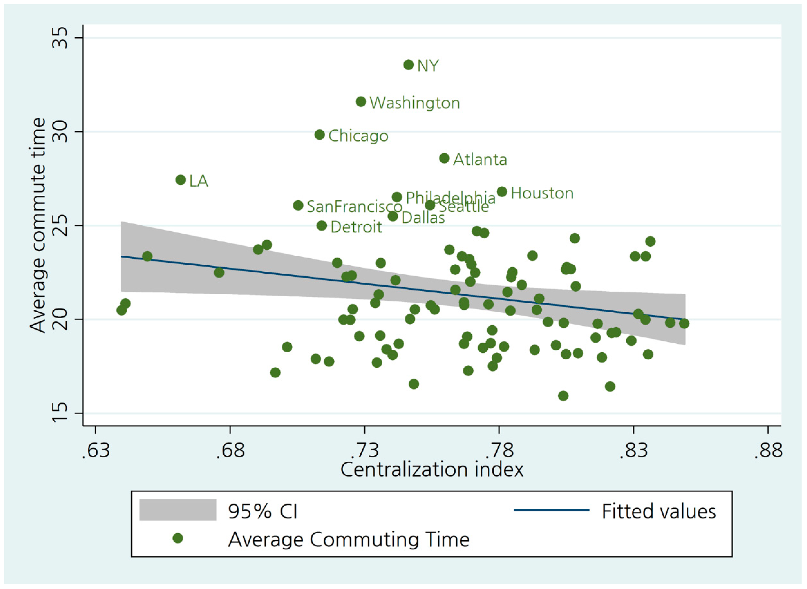
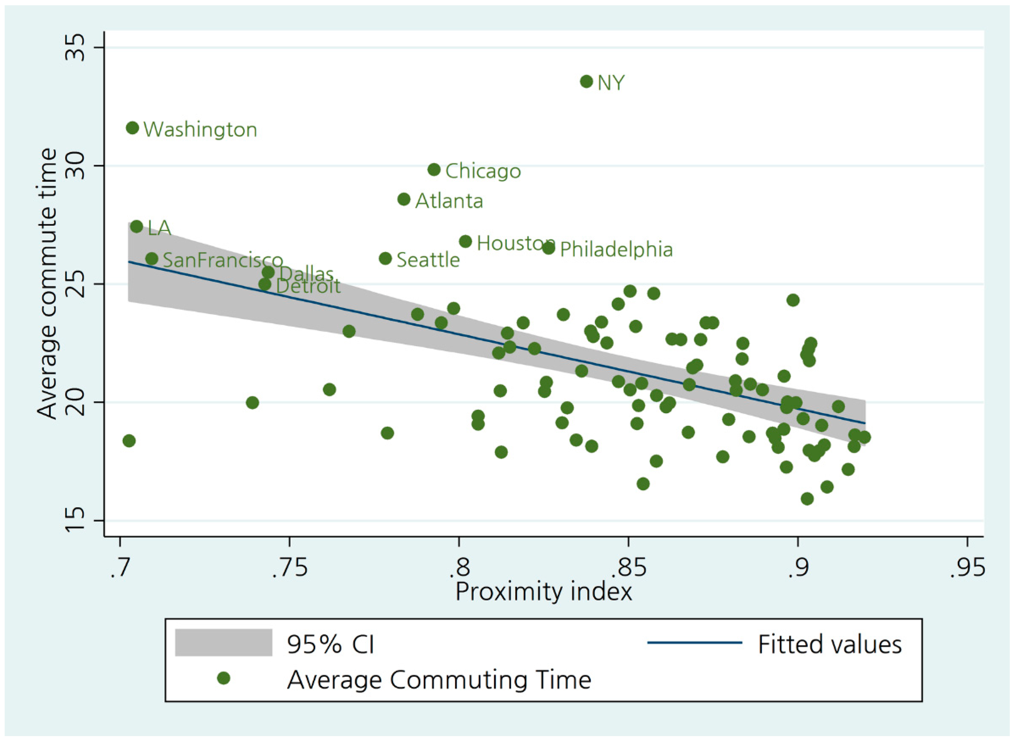
Table 1.
Variable description.
| Name | Description | Data Source |
|---|---|---|
| CT | Average commuting time | 2010 ACS |
| ACT | Average commuting time by auto | 2010 ACS |
| PJW | Job–worker proximity index | LODES |
| CJW | Centralization index | LODES |
| BPJW | Between estimator for extreme jobs and workers | LODES |
| NC | The number of employment clusters | LODES |
| JWCR | The ratio of the number of jobs in employment clusters to the metro jobs | LODES |
| JWCENTER | Job–worker ratio for the central business district (CBD) area | LODES |
| JWSUBURB | Job–worker ratio for the inner suburb ring (4–25 miles) | LODES |
| SMICENTER | Spatial mismatch index for the CBD area | LODES |
| SMISUBURB | Spatial mismatch index for the inner suburb ring (4–25 miles) | LODES |
| INCOME | Median household income | 2010 ACS |
| MULTI | The percentage of multi-earner households | 2010 ACS |
| POP | 2010 population (million) | Census |
| POPG | Population growth (2000–2010) | Census |
| AQUIFER | Percentage of MSA overlaying aquifers | Burchfield et al. (2006) |
| RUGGEDNESS | Terrain ruggedness index in MSA (m.) | Burchfield et al. (2006) |
| NGPLG | The number of general-purpose local governments | 2002 Census of Government |
Note: ACS (American Community Survey), LODES (LEHD Origin–Destination Employment Statistics).
Table 2.
Summary statistics.
| Variable | Obs | Mean | Standard Deviation | Min | Max |
|---|---|---|---|---|---|
| CT | 99 | 21.348 | 3.216 | 15.918 | 33.563 |
| ACT | 99 | 21.631 | 2.891 | 16.433 | 30.905 |
| PJW | 99 | 0.849 | 0.053 | 0.703 | 0.920 |
| CJW | 99 | 0.764 | 0.046 | 0.640 | 0.849 |
| BPJW | 99 | 0.170 | 0.101 | 0.004 | 0.509 |
| NC | 97 | 4.918 | 5.834 | 1.000 | 41.000 |
| JWCR | 97 | 0.294 | 0.084 | 0.062 | 0.490 |
| JWCENTER | 99 | 1.951 | 0.709 | 0.588 | 5.208 |
| JWSUBURB | 99 | 0.952 | 0.102 | 0.625 | 1.191 |
| SMICENTER | 99 | 58.782 | 6.028 | 43.220 | 73.101 |
| SMIISUBURB | 99 | 55.504 | 4.612 | 39.291 | 67.479 |
| INCOME | 99 | 42.033 | 5.658 | 31.530 | 65.500 |
| MULTI | 99 | 0.415 | 0.030 | 0.342 | 0.491 |
| POP | 99 | 2.076 | 3.161 | 0.395 | 21.942 |
| POPG | 99 | 0.130 | 0.105 | -0.108 | 0.409 |
| AQUIFER | 98 | 2425.874 | 3674.309 | 0.000 | 10000 |
| RUGGEDNESS | 98 | 172.954 | 352.381 | 0.002 | 2209.902 |
| NGPLG | 99 | 93.535 | 121.058 | 6.000 | 752 |
Table 3.
OLS regression (dependent variable: mean commuting time).
| (1) | (2) | (3) | (4) | (5) | (6) | |
|---|---|---|---|---|---|---|
| PJW | −7.132 * | −10.795 ** | −10.397 ** | −9.245 ** | −9.290 ** | −10.482 ** |
| (−1.71) | (−2.44) | (−2.23) | (−2.09) | (−2.11) | (−2.20) | |
| MULTI | −25.001 *** | −27.189 *** | −28.095 *** | −25.698 *** | −25.115 *** | −25.212 *** |
| (−3.64) | (−3.99) | (−4.14) | (−3.98) | (−3.89) | (−3.87) | |
| INCOME | 0.170 *** | 0.172 *** | 0.180 *** | 0.169 *** | 0.173 *** | 0.193 *** |
| (3.64) | (3.76) | (3.91) | (3.87) | (3.96) | (4.27) | |
| POP | 0.586 *** | 0.604 *** | 0.574 *** | 0.659 *** | 0.694 *** | 0.710 *** |
| (7.45) | (7.78) | (3.96) | (4.74) | (4.89) | (4.99) | |
| POPG | 3.267 * | 3.476 ** | 3.156 * | 1.146 | 1.410 | 1.271 |
| (1.84) | (1.99) | (1.78) | (0.65) | (0.79) | (0.71) | |
| CJW | 9.918 ** | 9.545 ** | 4.259 | 6.912 | 7.602 | |
| (2.17) | (2.08) | (0.93) | (1.36) | (1.49) | ||
| NC | 0.011 | −0.079 | −0.091 | −0.115 | ||
| (0.13) | (−0.93) | (−1.07) | (−1.33) | |||
| JWCR | 8.330 *** | 8.612 *** | 8.371 ** | |||
| (3.42) | (3.53) | (3.38) | ||||
| BPJW | −2.461 | −2.730 | ||||
| (−1.20) | (−1.32) | |||||
| AQUIFER | 0.000 | |||||
| (0.15) | ||||||
| RUGGEDNESS | −0.000 | |||||
| (−0.88) | ||||||
| Cons. | 28.983 *** | 25.258 *** | 25.347 *** | 25.970 *** | 23.862 *** | 23.854 *** |
| (6.30) | (5.23) | (5.00) | (5.42) | (4.69) | (4.57) | |
| N | 99 | 99 | 97 | 97 | 97 | 96 |
| Adj- | 0.679 | 0.691 | 0.693 | 0.726 | 0.728 | 0.729 |
Note: t-statistics in parentheses; * p < 0.1; ** p < 0.05; *** p < 0.001.
Table 4.
OLS regression (dependent variable: mean commuting time by auto).
| (1) | (2) | (3) | (4) | (5) | (6) | |
|---|---|---|---|---|---|---|
| PJW | −9.426 ** | −12.251 ** | −9.487 ** | −8.385 * | −8.429 * | −10.582 ** |
| (−2.31) | (−2.80) | (−2.10) | (−1.96) | (−1.97) | (−2.33) | |
| MULTI | −28.347 *** | −30.035 *** | −30.671 *** | −28.377 *** | −27.804 *** | −27.487 *** |
| (−4.21) | (−4.45) | (−4.66) | (−4.53) | (−4.44) | (−4.42) | |
| INCOME | 0.175 *** | 0.177 *** | 0.176 *** | 0.166 *** | 0.170 *** | 0.194 *** |
| (3.82) | (3.90) | (3.95) | (3.91) | (4.00) | (4.51) | |
| POP | 0.409 *** | 0.423 *** | 0.209 | 0.291 ** | 0.326 ** | 0.348 ** |
| (5.31) | (5.52) | (1.49) | (2.15) | (2.37) | (2.57) | |
| POPG | 4.890 ** | 5.051 ** | 4.955 ** | 3.031 * | 3.291 * | 3.153 * |
| (2.81) | (2.92) | (2.89) | (1.76) | (1.90) | (1.84) | |
| CJW | 7.649 * | 7.674 * | 2.617 | 5.226 | 6.298 | |
| (1.69) | (1.73) | (0.59) | (1.06) | (1.29) | ||
| NC | 0.139 * | 0.052 | 0.040 | 0.008 | ||
| (1.67) | (0.63) | (0.49) | (0.10) | |||
| JWCR | 7.970 ** | 8.248 *** | 8.060 *** | |||
| (3.37) | (3.48) | (3.41) | ||||
| BPJW | −2.420 | −2.870 | ||||
| (−1.22) | (−1.45) | |||||
| AQUIFER | 0.000 | |||||
| (0.28) | ||||||
| RUGGEDNESS | −0.001 | |||||
| (−1.62) | ||||||
| Cons. | 32.543 *** | 29.671 *** | 27.409 *** | 28.005 *** | 25.932 *** | 26.173 *** |
| (7.22) | (6.22) | (5.58) | (6.02) | (5.25) | (5.26) | |
| N | 99 | 99 | 97 | 97 | 97 | 96 |
| Adj- | 0.619 | 0.626 | 0.641 | 0.678 | 0.680 | 0.690 |
Note: t-statistics in parentheses; * p < 0.1; ** p < 0.05; *** p < 0.001.
Table 5.
2SLS estimation (full model; dependent variable: mean commuting time).
| (1) | (2) | (3) | (4) | (5) | (6) | |
|---|---|---|---|---|---|---|
| PJW | 10.314 | 4.111 | −14.974 | −13.614 | −12.746 | −122.715 |
| (0.73) | (0.28) | (−1.22) | (−1.17) | (−1.11) | (−1.25) | |
| MULTI | −28.30 *** | −28.54 *** | −28.83 *** | −26.46 *** | −25.88 *** | −18.32 |
| (−3.78) | (−4.13) | (−4.45) | (−4.30) | (−4.24) | (−1.02) | |
| INCOME | 0.233 *** | 0.221 *** | 0.193 *** | 0.180 *** | 0.185 *** | 0.086 |
| (3.77) | (3.93) | (4.01) | (3.96) | (4.12) | (0.58) | |
| POP | 0.666 *** | 0.648 *** | 0.612 *** | 0.687 *** | 0.719 *** | 1.175 ** |
| (5.91) | (6.64) | (4.09) | (4.86) | (5.04) | (2.15) | |
| POPG | 2.568 | 2.781 | 2.898 * | 1.080 | 1.325 | 2.898 |
| (1.35) | (1.53) | (1.70) | (0.63) | (0.78) | (0.60) | |
| CJW | 4.315 | 11.041 * | 6.028 | 8.415 | 46.111 | |
| (0.61) | (1.91) | (1.03) | (1.37) | (1.28) | ||
| NC | −0.041 | −0.119 | −0.126 | −0.749 | ||
| (−0.38) | (−1.16) | (−1.24) | (−1.26) | |||
| JWCR | 7.756 ** | 8.079 *** | 3.942 | |||
| (3.27) | (3.43) | (0.53) | ||||
| BPJW | −2.514 | −3.766 | ||||
| (−1.30) | (−0.69) | |||||
| AQUIFER | −0.000 | |||||
| (−0.92) | ||||||
| RUGGEDNESS | −0.005 | |||||
| (−1.19) | ||||||
| Cons. | 12.869 | 15.426 | 28.081 ** | 28.525 *** | 25.767 ** | 95.899 |
| (0.98) | (1.56) | (3.12) | (3.36) | (3.03) | (1.49) | |
| N | 98 | 98 | 96 | 96 | 96 | 96 |
Note: t-statistics in parentheses; * p < 0.1; ** p < 0.05; *** p < 0.001.
Table 6.
2SLS estimation (variable selection).
| (1) | (2) | (3) | (4) | (5) | (6) | |
|---|---|---|---|---|---|---|
| Dep. Var.: Mean Comm. Time | Dep. Var.: Mean Comm. Time (Auto) | |||||
| PJW | −65.920 *** | −40.476 ** | −35.773 ** | −44.081 *** | −18.721 | −17.103 |
| (−4.01) | (−2.65) | (−2.24) | (−3.49) | (−1.61) | (−1.36) | |
| CJW | 16.788 | 12.379 | 10.387 | 5.651 | 2.206 | 1.976 |
| (1.32) | (1.29) | (1.04) | (0.58) | (0.30) | (0.25) | |
| MULTI | −15.394 | −29.468 *** | −29.380 *** | −16.039 * | −31.708 *** | −31.359 *** |
| (−1.39) | (−3.32) | (−3.44) | (−1.89) | (−4.69) | (−4.67) | |
| JWCR | 7.234 | 6.747 ** | 6.939 * | 10.194 ** | 9.349 *** | 8.968 ** |
| (1.58) | (1.99) | (1.96) | (2.90) | (3.62) | (3.22) | |
| BPJW | 2.527 | 0.837 | 0.706 | 1.593 | −0.288 | −0.534 |
| (0.70) | (0.31) | (0.27) | (0.58) | (−0.14) | (−0.26) | |
| INCOME | 0.248 *** | 0.263 *** | 0.268 *** | 0.275 *** | ||
| (3.53) | (3.80) | (5.00) | (5.06) | |||
| POPG | 0.888 | 1.801 | ||||
| (0.35) | (0.91) | |||||
| Cons. | 68.344 *** | 45.998 *** | 42.688 *** | 58.181 *** | 35.140 *** | 33.407 *** |
| (6.22) | (4.13) | (3.85) | (6.90) | (4.14) | (3.84) | |
| Excluded? | F = 10.14 (p = 0.000) | F = 6.84 (p = 0.002) | F = 5.73 (p = 0.005) | F = 10.14 (p = 0.000) | F = 6.84 (p = 0.002) | F = 5.73 (p = 0.005) |
| Exogenous? | = 12.07 (p = 0.001) | = 4.50 (p = 0.034) | = 4.50 (p = 0.109) | = 4.864 (p = 0.027) | = 0.37 (p = 0.543) | = 0.135 (p = 0.714) |
| N | 96 | 96 | 96 | 96 | 96 | 96 |
Note: t-statistics in parentheses; * p < 0.1; ** p < 0.05; *** p < 0.001. The first equations for Models (2) and (4) can be found in A.15 and A.16 in the Supplementary Materials. The two instrumental variables (NGPLG and RUGGEDNESS) are negatively associated with the job–worker proximity (PJW) and are statistically significant, which is as hypothesized.
Table 7.
OLS regression for city center and suburb (job–worker ratio and spatial mismatch index (SMI)).
Table 7.
OLS regression for city center and suburb (job–worker ratio and spatial mismatch index (SMI)).
| (1) | (2) | (3) | (4) | |
|---|---|---|---|---|
| Dep. Var.: Mean Commuting Time | ||||
| JWCENTER | 1.485 *** | 1.407 ** | 0.943 ** | 0.755 ** |
| (3.48) | (3.28) | (3.23) | (2.56) | |
| JWSUBURB | 1.648 | 1.829 | 3.039 | 3.341 * |
| (0.56) | (0.63) | (1.54) | (1.70) | |
| SMICENTER | 0.084 * | 0.104 * | 0.019 | 0.007 |
| (1.66) | (1.98) | (0.51) | (0.19) | |
| SMISUBURB | 0.186 ** | 0.193 ** | 0.099 ** | 0.065 |
| (2.74) | (2.85) | (2.12) | (1.28) | |
| MULTI | −12.557 | −17.915 ** | −16.885 ** | |
| (−1.36) | (−2.86) | (−2.72) | ||
| POP | 0.675 *** | 0.672 *** | ||
| (10.61) | (10.80) | |||
| JWCR. | 4.690 * | |||
| (1.71) | ||||
| Cons. | 1.580 | 5.259 | 16.074 *** | 16.928 *** |
| (0.41) | (1.12) | (4.83) | (5.12) | |
| N | 99 | 99 | 99 | 97 |
| Adj- | 0.330 | 0.336 | 0.698 | 0.710 |
Note: t-statistics in parentheses; * p < 0.1; ** p < 0.05; *** p < 0.001.
Table 8.
OLS regression for city center and suburb (job–worker ratio).
| (1) | (2) | (3) | (4) | |
|---|---|---|---|---|
| Dep. Var.: Mean Commuting Time | ||||
| JWCENTER | 2.087 *** | 2.087 *** | 1.122 *** | 0.790 ** |
| (5.22) | (5.20) | (4.12) | (2.79) | |
| JWSUBURB | 5.953 ** | 6.133 ** | 4.870 ** | 4.212 ** |
| (2.14) | (2.17) | (2.67) | (2.29) | |
| MULTI | −4.381 | −16.063 ** | −15.622 ** | |
| (−0.47) | (−2.62) | (−2.64) | ||
| POP | 0.711 *** | 0.689 *** | ||
| (11.56) | (11.57) | |||
| JWCR | 6.378 ** | |||
| (2.65) | ||||
| Cons. | 11.611 *** | 13.257 ** | 19.711 *** | 19.020 *** |
| (4.37) | (3.00) | (6.78) | (6.76) | |
| N | 99 | 99 | 99 | 97 |
| Adj- | 0.259 | 0.253 | 0.688 | 0.711 |
Note: t-statistics in parentheses; * p < 0.1; ** p < 0.05; *** p < 0.001.
Table 9.
OLS regression for city and suburb (spatial mismatch).
| (1) | (2) | (3) | (4) | |
|---|---|---|---|---|
| Dep. Var.: Mean Commuting Time | ||||
| SMICENTER | 0.153 ** | 0.174 *** | 0.065 * | 0.043 |
| (3.10) | (3.45) | (1.81) | (1.17) | |
| SMISUBURB | 0.245 *** | 0.253 *** | 0.151 *** | 0.099 * |
| (3.81) | (3.96) | (3.40) | (1.97) | |
| MULTI | −16.383 * | −20.345 ** | −18.196 ** | |
| (−1.71) | (−3.12) | (−2.84) | ||
| POP | 0.700 *** | 0.688 *** | ||
| (10.57) | (10.78) | |||
| JWCR | 6.358 ** | |||
| (2.29) | ||||
| Cons. | −1.237 | 3.877 | 16.126 *** | 17.591 *** |
| (−0.33) | (0.81) | (4.66) | (5.18) | |
| N | 99 | 99 | 99 | 97 |
| Adj- | 0.257 | 0.272 | 0.664 | 0.686 |
Note: t-statistics in parentheses; * p < 0.1; ** p < 0.05; *** p < 0.001.
© 2019 by the authors. Licensee MDPI, Basel, Switzerland. This article is an open access article distributed under the terms and conditions of the Creative Commons Attribution (CC BY) license (http://creativecommons.org/licenses/by/4.0/).
Share and Cite
MDPI and ACS Style
Kim, C.; Choi, C. Towards Sustainable Urban Spatial Structure: Does Decentralization Reduce Commuting Times? Sustainability 2019, 11, 1012. https://0-doi-org.brum.beds.ac.uk/10.3390/su11041012
AMA Style
Kim C, Choi C. Towards Sustainable Urban Spatial Structure: Does Decentralization Reduce Commuting Times? Sustainability. 2019; 11(4):1012. https://0-doi-org.brum.beds.ac.uk/10.3390/su11041012
Chicago/Turabian StyleKim, Chunil, and Choongik Choi. 2019. "Towards Sustainable Urban Spatial Structure: Does Decentralization Reduce Commuting Times?" Sustainability 11, no. 4: 1012. https://0-doi-org.brum.beds.ac.uk/10.3390/su11041012
Note that from the first issue of 2016, this journal uses article numbers instead of page numbers. See further details here.