Classifying Urban Climate Zones (UCZs) Based on Spatial Statistical Analyses ^†

Abstract

The objective of this study is the classification of urban climate zones (UCZs) based on spatial statistical approaches to provide key information for the establishment of thermal environments to improve urban planning. To achieve this, using data from 246 automatic weather stations (AWSs), air temperature maps in the summer of the study area were prepared applying universal kriging interpolation analysis. In addition, 22 preliminary variables to classify UCZs were prepared by a 100 m × 100 m grid. Next, six influential urban spatial variables to classify UCZs were finalized using spatial regression analysis between air temperature and preliminary variables. Finally, the UCZs of the study area were delineated by applying K-mean clustering analysis, and each spatial characteristic of the UCZs was identified. The results found that the accuracy of the air temperature of the study area ranged from ±0.184 °C to ±0.824 °C with a mean 0.501 root mean square predict error (RMSPE). Elevation, normalized difference vegetation index (NDVI), commercial area, average height of buildings, terrain roughness class, building height to road width (H/W) ratio, distance from subway stations, and distance from water spaces were identified as finalized variables to classify UCZs. Finally, a total of 8 types of UCZs were identified and each zone showed a different urban spatial pattern and air temperature range. Based on the spatial statistical analysis results, this study delineated clearer UCZs boundaries by applying influential urban spatial elements that resulted from previous classification studies of UCZs mainly based on pre-determined spatial variables. The methods presented in this study can be effectively applied to other cities to establish urban heat island counter measures that have similar weather observation conditions.

1. Introduction

The urban heat island (UHI) phenomenon has been recognized as a negative side effect of rapid urbanization. The main causes of the urban heat island phenomenon include trapping of short and long wave radiation between buildings, decreasing of long-wave radiative heat losses due to building construction, increasing storage of sensible heat in the construction materials of buildings and structures, anthropogenic heat released from human activities, and reduction of evapotranspiration potential [1,2]. Various attempts have been made to mitigate UHI through urban planning and design. In order to achieve effective urban heat island mitigation, it is necessary to understand and apply urban climatic information in urban planning [3].

In this regard, the urban climate zone (UCZ) concept is useful as a UHI mitigation measure because it offers integrated information on climate characteristics and related spatial elements [4]. UCZs are homogeneously classified areas that distinguish climate characteristics based on urban structure, land cover, urban fabric, and urban metabolism [5]. Considered fundamental research on UCZ, Chandler [6], Auer Jr. [7], Ellefsen [8], and Oke [5] established the concept of UCZ and suggested major variables including topography, land cover, building forms, etc., to classify UCZs. Recently, as empirical studies, Houet and Pigeon [9] investigated the usefulness of the UCZ concept as a tool to understand climate phenomena, and Lee and Oh [3] identified influential variables to classify UCZs and delineated UCZs boundaries based on statistical analyses.

Meanwhile, in order to analyze the urban heat island phenomenon, precise air temperature maps should be prepared as much as possible. In the case of Korea, due to its complex topographical situations and diverse meteorological elements with much spatial and temporal variations, a large number of stations are needed to quantitatively sense local climate characteristics. Since it is practically difficult to prepare high resolution meteorological data by installing observation stations, interpolation methods have been frequently employed. Generally, they calculate point data by weighing inversely and proportional to the square of distance, assuming that the homogeneity of meteorological elements decreases with distance. However, these methods alone have limitations in obtaining good quality, precise, and high-resolution data. Most of the meteorological elements, including air temperature, are affected not only by distance but also by the surrounding topographical environment, such as elevation. Therefore, in order to prepare a precise and high-resolution air temperature map that can represent local climate characteristics, it is necessary to develop a more effective spatial interpolation method considering the influence of diverse meteorological elements such as topography in addition to distance [10,11]. In this regard, interpolation methods that consider topographical factors such as elevation, slope, and aspect are needed for urban heat island research [11].

Meanwhile, statistical approaches applying multiple regression analysis have been applied to identify the relationship between UHI and urban spatial characteristics. However, the statistical approach has limitations in presenting several physical phenomena [12]. The major reason for the limitation is that installing climate measurement devices in entire urban areas is impossible due to space constraints, installation time, and expensive operating costs. This lack of observational data makes it difficult to analyze the relationship between the urban heat island phenomena and urban spatial characteristics. Another reason is that conventional regression analysis, such as the ordinary least squares (OLS) model, is based on the assumption that observations are independent, resulting in a failure to capture the spatial dependence of data when they are applied to geo-referenced datasets [13]. Therefore, spatial regression analysis has been recently used to explain UHI, according to spatial neighborhood effects [1].

In order to classify UCZs more accurately, it is essential to conduct in-depth investigation on the relationship between urban climate changes and urban spatial elements through systematic and scientific analysis. Therefore, the aims of this study are to: (1) identify influential urban spatial elements to classify UCZs based on spatial statistical analyses, (2) delineate UCZs boundaries, and (3) provide key information for urban planning and design to establish UHI mitigation measures.

2. Materials and Methods

This study consists of four parts and each process is presented in Figure 1. First, observation data were obtained from 246 automatic weather stations (AWSs), which were observed on cloudless days with a gentle breeze speed (less than 5.4 m/s, based on Beaufort Wind Scale). Using these data, air temperature maps of the study area were prepared by a universal kriging interpolation method. Next, preliminary independent variables were prepared, including topography, land use, land cover, urban form, human activities, and locational characteristics, to predict air temperature. Third, influential urban spatial elements were identified to classify UCZs by spatial regression analysis. Finally, UCZ boundaries in the study area were delineated by K-mean clustering analysis. In addition, the spatial characteristics of each UCZ were investigated.

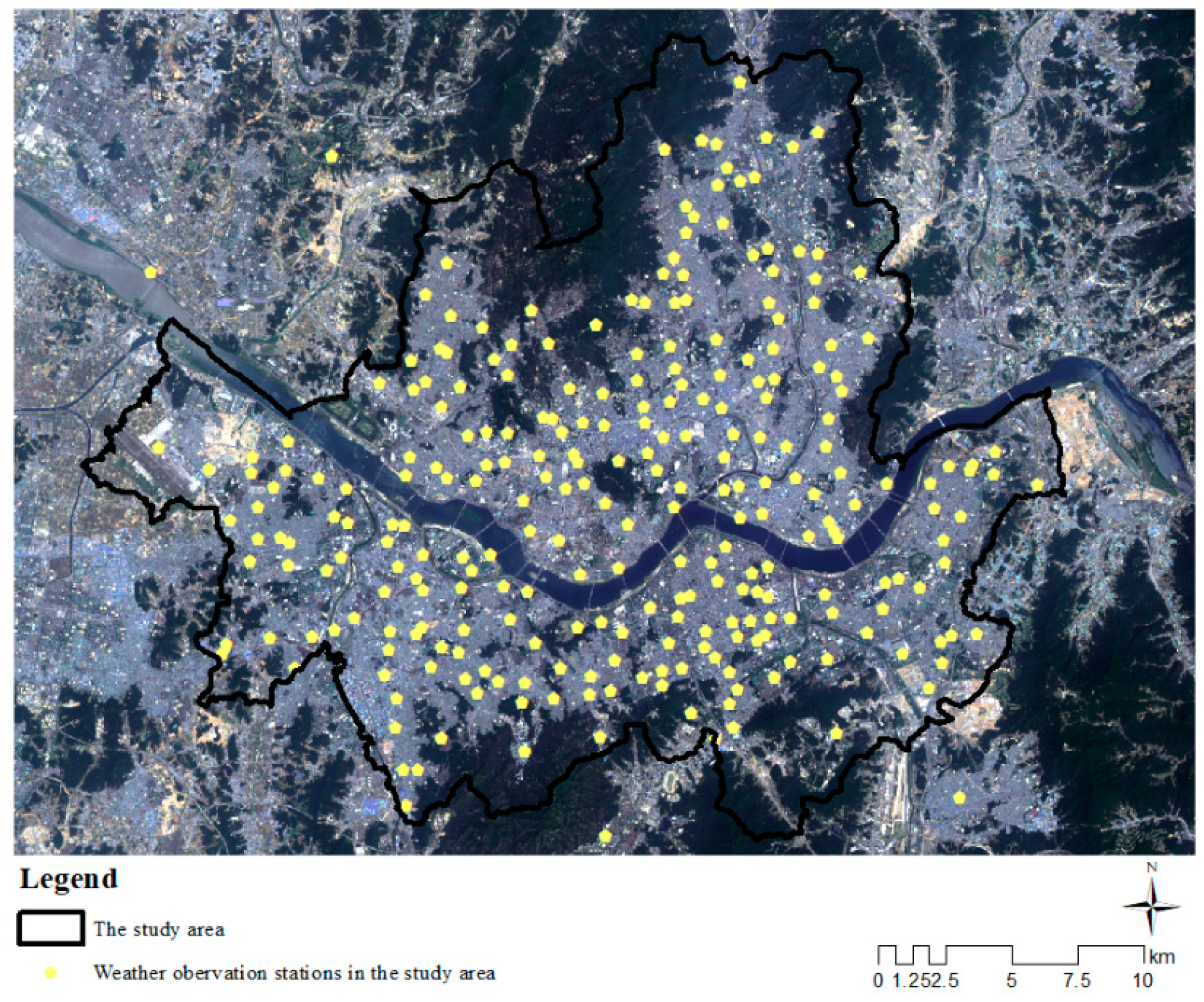
A case study was conducted for Seoul, the capital of South Korea. Seoul is one of the densest cities in the world in which 21.5% (about 11 million inhabitants) of the country’s total population reside. Seoul is also a representative heat island city that has diverse spatial characteristics including land cover, land use, building form, etc. In the case of South Korea, weather information was investigated by 26 AWSs (automatic weather stations), which are operated by the Korea Meteorological Administration (KMA), and the average distance of each weather station is approximately 3 km in the study area. It is very difficult to classify UCZs of metropolitan cities using such a resolution. Therefore, additional weather data collected by 220 AWSs of a Korean private company (SK Weather Planet) were integrated into the analysis in this study (Figure 2). Among the 246 weather stations, 26 of the AWSs were used to verify the air temperature analysis results. Eventually, 220 of the AWSs were actually used to prepare the air temperature map.

2.1. Analysis of Air Temperature

Urban heat island intensity has commonly been defined as the temperature difference between urban and rural places [14]. In a metropolitan city, the air temperature based UHI is reported to be high and positive during nighttime (2–3 h after sunset) for cloudless days and light winds [15,16]. Considering such characteristics of an urban heat island, analysis time points were selected to classify UCZs. In order to take into account the climate characteristics, three days per month in summer (from June to August) with the lowest cloudiness and the lowest wind speed were investigated. Subsequently, considering sunset times and weather conditions (under a cloudless sky and gentle breeze wind speed), 10:00 p.m. and 11:00 p.m. of 9 days in each summer in 2015 and 2016 were chosen for statistical analyses (

Table 1. Weather conditions for the 18 days in 2015 and 2016.

		Min Air Temperature	Max Air Temperature	Mean Air Temperature	Mean Wind Speed	Mean Amount of Cloud (1–10)
2015	6 June	18.8 °C	31.1 °C	24.4 °C	2.4 m/s	1.4
	14 June	18.3 °C	37.7 °C	22.5 °C	3.3 m/s	3.9
	30 June	21.2 °C	30.2 °C	25.3 °C	2.7 m/s	3.4
	4 July	21.6 °C	32.3 °C	26.8 °C	2.4 m/s	3.6
	27 July	21.4 °C	30.6 °C	25.0 °C	1.9 m/s	4
	29 July	30.1 °C	33.5 °C	28.6 °C	2.5 m/s	2.5
	8 August	26.1 °C	30.6 °C	26.1 °C	3.8 m/s	2.1
	28 August	19.8 °C	30.7 °C	25.1 °C	2.2 m/s	1.6
	30 August	19.9 °C	30.7 °C	24.6 °C	1.9 m/s	2.4
2016	5 June	17.3 °C	32.2 °C	24.7 °C	1.7 m/s	3.5
	9 June	17.8 °C	31.3 °C	24.1 °C	2.0 m/s	1.4
	19 June	20.3 °C	29.3 °C	1.90 °C	2.7 m/s	4.4
	8 July	27.3 °C	21.2 °C	2.4 °C	1.8 m/s	0.1
	9 July	27.7 °C	23.2 °C	33.1 °C	1.8 m/s	3.1
	19 July	20.9 °C	32.4 °C	27.1 °C	1.5 m/s	3.6
	5 August	26.5 °C	36.0 °C	31.2 °C	1.8 m/s	1.9
	10 August	26.1 °C	34.8 °C	29.4 °C	1.9 m/s	4.4
	17 August	25.1 °C	34.7 °C	29.9 °C	1.9 m/s	2.4

).

Meanwhile, the average spacing of the AWSs in the case study area is 1087 m, which is much shorter than other metropolises. To analyze the air temperature, statistical interpolation methods are commonly used to prepare temperature maps using point-based measurements. IDW (Inverse Distance Weighting) of Shepard [17], Kriging [18], and Spline [19] are representative statistical interpolation methods. However, although the average spacing of the AWSs is much shorter than in other cities, these methods still have limitations in that they do not effectively reflect the heterogeneity of urban spatial characteristics that include the influence of land cover and elevation on temperature. Therefore, in this study, the universal kriging interpolation method based on the GPR (Gaussian process regression) model was applied in order to consider variables such as altitude, distance to coast or river, and water space area ratio besides the distance between measurement points. The universal kriging, an unbiased linear estimator with minimum estimation variance properties, was used based upon the theory of regionalized variables [20]. The GPR model is generally constructed as follows:

$$y=F\beta +Z\left(X\right)+e$$

(1)

where F is the designed matrix, B is the regression coefficient, Z(X) is the Gaussian stochastic process, which shows an average of 0, and ${\mathsf{\sigma }}_Z^{2}R\left(X\right)$ the variance–covariance matrix, and e is the normal distributed observational error that shows an average of 0 and ${\mathsf{\sigma }}_e^2$ variance. Based on the GPR model, additional explanatory variables were inputted in the universal kriging interpolation method and the equation is as follows:

$$y={\beta }_0+{\beta }_2\left(elevation\right)+{\beta }_2\left(distance from water space\right)+{\beta }_3\left(water space area ratio\right)+Z\left(X\right)+e$$

(2)

The Z(X) is determined by latitude and longitude coordinates. To determine the appropriate interpolation methods, data from 220 AWSs were interpolated using universal kriging interpolation methods and they were compared with data from 26 AWSs. The results found that the root mean square predict error (RMSPE) by the universal kriging interpolation method ranged from ±0.184 °C to ±0.824 °C with a mean 0.501 °C. Among the 36 analysis time points, 10 time points that showed the relatively low RMSPE (less than 0.45) were selected to delineated air temperature (

Table 2. Ten time points to prepare air temperature analysis (RMSPE < 0.45).

		Min (°C)	Max (°C)	Mean (°C)	SD	RMSPE
2015	12 p.m., 6 June	15.330	24.021	21.890	1.320	0.390
	10 p.m., 1 July	15.124	23.133	21.569	1.034	0.439
	10 p.m., 27 July	22.330	29.242	27.897	0.921	0.428
	11 p.m., 27 July	24.356	28.327	27.258	1.021	0.435
	10 p.m., 30 July	24.745	29.756	27.235	1.243	0.325
2016	10 p.m., 5 June	16.312	25.021	22.814	1.245	0.371
	10 p.m., 8 July	16.532	25.721	23.024	1.221	0.390
	11 p.m., 10 August	29.751	29.751	28.019	1.251	0.184
	10 p.m., 17 August	31.211	31.211	29.149	1.383	0.203
	11 p.m., 17 August	30.714	30.714	27.571	1.320	0.260

). Thus, 10 air temperature maps of 2 and 3 h after sunset were prepared, and finally, an average air temperature map was calculated from these maps.

2.2. Selection of Preliminary Variables

Adopting the research of Lee and Oh [3], this study classified urban spatial elements into 6 categories including topology, land use, land cover, building characteristics, human activity, and locational characteristics. The number of total preliminary variables was 22 (

Table 3. The preliminary variables for the air temperature predicting model (adopted from Lee and Oh [3]).

Categories	Variables (Unit)
Topography	Slope (degree), elevation (m)
Land use	Residential, commercial, industrial, green space, water space area ratio (%)
Land cover	Impervious surface area ratio (%), albedo (0 to1), NDVI (0 to 1)
Urban form	Average width of buildings (m), average height of buildings (m), the number of buildings, building surface fraction (%), floor area ratio (%), H/W ratio (number), terrain roughness class (number)
Human activities	Population (person), number of vehicles (number)
Locational characteristics	Distance from green spaces (m), distance from water spaces (m), distance from subway stations (m)

). Meanwhile, determining spatial resolution was important in order to identify influential variables and delineate UCZs boundaries. Considering the research of Houet and Pigeon [9] and Lee and Oh [3], this study prepared preliminary variables to classify UCZs using a 100 m grid resolution.

2.3. Identification of Influential Urban Spatial Elements to Classify UCZs

To select independent variables for an air temperature prediction model, correlation analysis was conducted to investigate the interrelationship between preliminary variables and air temperature. The potential multi-collinearity among the preliminary variables were also identified. Based on correlation analysis, ordinary least squares (OLS) regression analysis was applied. In order to reduce the heteroscedastic effect of wide ranging preliminary variables, the logarithm of the dependent variable, Ln (air temperature), was used. A step-wise regression analysis method (forward selection approach) was applied to find influential variables that would affect air temperature. Since the air temperature map was delineated by the interpolation method, the spatial lag model (SLM) was next estimated to control the effects of air temperature in neighboring grids.

2.4. UCZ Classification

Using the influential urban spatial elements identified, the UCZs of the study area were classified by mean clustering analysis. Since this study had a large number of samples (N: 52,961), K-mean clustering analysis was applied due to its efficacy of ascertaining clusters within large quantities of data [21]. For the K-mean clustering analysis, the Z-scores of the influential variables identified by regression analysis were calculated. The calculated Z-scores were inputted as parameters for cluster analysis, and iterative calculations were performed until the adjustment of the centroids of the clusters did not occur after setting the centroids of the initial clusters.

On the other hand, one of the most important points in applying K-mean cluster analysis is determining K (the appropriate number of clusters). Oke [5] classified UCZs as 7 categories, and in the case of Ellefsen [8] UTZs (urban terrain zones) were classified as 9 categories. Considering such previous studies, the preliminary number of classes for K-mean clustering analysis (K) was determined from 6 to 12 (total 7 cases), and the appropriate number of K was chosen by sensitivity analysis using the ANOVA test. Thus, in the ANOVA test, the dependent variables were Ln (air temperature), and factorial variables were the cases of clusters. The F values of 7 ANOVA tests were investigated to determine whether the distribution of Ln (air temperature) in each cluster were statistically significant. A case with the highest F value among the 7 cases was chosen as the final K to classify the UCZs. Then, characteristics of each UCZ were determined based on the chosen K-mean clustering analysis results. Finally, the UCZs maps were prepared to explain the actual air temperature phenomenon.

3. Results

3.1. Air Temperature

Figure 3 presents air temperature maps of the study area. Air temperatures ranged from 24.14 °C to 30.46 °C with an average value of 27.23 °C. The maximum temperature differences were analyzed and found to be more than 6.32 °C. This confirmed that the urban heat island phenomenon was relatively severe in the study area.

3.2. Identification of Influential Urban Spatial Elements to Classify UCZs

Table 4. Correlation analysis results between air temperature and urban spatial elements.

Categories	Correlation Coefficients
Topography	Elevation (−0.681 **), slope (−0.621 **)
Land use	Green space (−0.501 **), commercial (0.310 **), residential (0.284 **), industrial (0.037 **)
Land cover	Impervious surface area ratio (0.552 **), NDVI (−0.603 **), albedo (−0.461 **)
Urban form	Sky view factor (SVF) (−0.400 **), average width of buildings (0.356 **), average height of buildings (0.309 **), the number of buildings (0.331 **), building surface fraction (0.437 **), terrain roughness class (0.559 **), H/W ratio (0.187 **)
Locational characteristics	Distance from green spaces (0.411 **), distance from subway stations (−0.670 **), distance from water spaces (−0.047 **)

N: 52,961, **: p < 0.01.

shows the correlation analysis results of air temperature and urban spatial elements. The most positively correlated variable was the impervious surface area ratio, whereas the elevation showed the most negative correlation. In order to create a model to predict air temperature, variables that had strong correlations were inputted for step-wise regression analysis. In order to create a model to predict air temperature, the variables that had strong correlations were inputted for the step-wise regression analysis using the statistical software (SPSS 21). The estimated model showed 0.603 of R² and eight variables were found to be significant at the 99% level and had signs consistent with the results of the correlation analysis. In addition, due to the multi-collinearity diagnosis, all VIFs of the dependent variables were found to be less than three, and it was confirmed that there was no multi-collinearity problem in the models.

However, as a result of the Lagrange multiplier diagnostics for spatial dependence, it was found that the OLS error terms were spatially auto-correlated. In order to reduce this spatial auto correlation, SLM was next estimated to control the effects of air temperature in neighboring grids. The results showed that R² of SLM increased to 0.828, and coefficients of the independent variables had the same signs as in the OLS models. In addition, eight variables were all significant at the 1% level. Therefore, eight variables, including elevation, NDVI, commercial area, average height of buildings, terrain roughness class, H/W ratio, distance from subway stations, and distance from water spaces were included as significant variables to classify UCZs (

Table 5. Results of regression analysis (OLS and SLM).

		OLS		SLM
		Coefficient	t	Coefficient	z
T	Elevation	−1.914 × 10−4 ***	−85.345	−9.936 × 10−5 ***	−58.788
LU	Commercial	4.252 × 10−7 ***	−15.332	1.775 × 10−7 ***	4.435
LC	NDVI	−0.036 ***	−15.332	−0.015 ***	−10.655
UF	TRC	0.027 ***	45.107	0.010 ***	27.525
	AHB	8.861 × 10−5 ***	8.548	3.561 × 10−7 ***	4.938
	H/W	1.982 × 10−4 ***	6.504	1.982 × 10−4 ***	4.585
LoC	DS	−1.775 × 10−5 ***	−69.509	−7.893 × 10−5 ***	−44.6821
	DW	4.204 × 10−6 ***	19.503	2.544 × 10−6 ***	17.2331
	constant	3.353 ***	3783.853	1.542	162.049
	ρ		-	0.540	190.521
	Log-likelihood		112,643	133,591
	R2		0.603	0.828

N: 52,961, ***: Statistically significant at the 1% level. (T: Topography, LU: Land Use, LC: Land Cover, UF: Urban Form, LoC: Locational Characteristics, TRC: Terrain Roughness Class, AHB: Average Height of Buildings, DS: Distance from Subway Station, DW: Distance from Water spaces).

).

3.3. The Results of UCZ Classification

The seven cases of ANOVA test results showed that each clustered result was in a statistically different group. In the case of the variations of F values, it was confirmed that the F values were the highest when the number of cluster (K) was eight. In addition, when the number of clusters was larger than nine, it was found that the F values decreased (Appendix A). Based on the results of this sensitivity analysis, this study found that the appropriate number of clusters for UCZs was eight. Based on the selected clustering analysis results (

Table 6. Classification results of UCZs.

Cluster Factor	Cluster
	1 (N: 4868)	2 (N: 40)	3 (N: 183)	4 (N: 13,843)	5 (N: 1214)	6 (N: 20,007)	7 (N: 4280)	8 (N: 8526)
Elevation	2.583	−0.000	−0.039	0.121	−0.183	−0.390	−0.444	−0.506
DS	1.988	0.062	−0.075	0.412	−0.203	−0.400	−0.468	−0.599
TRC	−1.154	−0.187	−0.155	−1.164	0.142	0.616	0.522	0.825
DW	0.471	0.113	0.052	−0.173	0.220	0.102	−0.405	−0.058
NDVI	1.483	0.621	0.501	0.957	0.048	−0.573	−0.411	−0.870
H/W ratio	−0.491	18.211	9.461	−0.410	2.692	0.050	0.200	0.056
Commercial	−0.525	−0.528	−0.460	−0.500	−0.432	−0.284	−0.311	2.010
AHB	−0.749	3.673	2.157	−0.639	1.546	−0.066	2.415	0.125

and Figure 4), UCZs could be classified into mountainous areas (cluster 1), hilly areas and urban forest (cluster 4), high-rise built up areas with very a high H/W ratio (cluster 3), mid-rise built up areas with a high H/W ratio (cluster 5), mid-rise built up areas without green spaces (cluster 6), high-rise built up areas with a high H/W ratio (cluster 2), high-rise built up areas with various building heights (cluster 7), and commercial areas without green spaces (Figure 5). As a result, the classification of UCZs in this study showed similar spatial patterns with the air temperature analysis results.

4. Discussion and Conclusions

Through a series of statistical analyses, this study identified more detailed and clearer UCZ boundaries (100 m × 100 m) and explained statistically significant urban spatial characteristics to understand urban climate phenomena. Through spatial regression analyses, influential urban spatial elements causing air temperature increases and their effects were concretely investigated. In addition, the potential areas where urban heat islands occur were delineated using UCZ maps.

The UCZ classification based on spatial statistical analyses conducted in this study has usefulness as follows: First, this study produced an air temperature map that shows relatively high accuracy using an interpolation method. Due to a lack of observation data, the conventional interpolation method to delineate urban air temperature was robust. As a result, it was difficult to analyze the relationship between air temperature and urban spatial characteristics. In fact, most of the previous studies used land surface temperature data in identifying the effects of urban spatial characteristics. By applying a number of AWS data, this study overcame such a limitation, and the actual sensed effects on air temperature were investigated. In addition, using a number of AWS data, applying the universal kriging interpolation method, which considers the effects of elevation and water space, more accurate air temperature maps (RMSPE: from ±0.184 °C to ±0.824 °C) were delineated. Such an air temperature analysis method will enhance the efficiency and accuracy of investigating climate phenomena. Since some interpolated results showed a relatively high RMSPE, there is some need for improvement of the universal kriging interpolation methods presented in this study of 100 m spatial resolution at AWS spacing of 1087 m. In order to reflect the heterogeneity of urban spaces, the spacing of AWSs still should be shortened. Recently, with advances and the dissemination of more economic smart sensing technologies, more AWSs are being installed. If such data is accumulated and obtained, accuracy and precision by universal kriging methods are expected to be further improved.

Second, by applying spatial regression analysis, influential variables that affect air temperature were identified, and their effects on air temperature were investigated. Thus, this study suggested integrated information on climate characteristics and related urban spatial elements. The outcomes of this study can provide urban planners with practical information to improve the urban thermal environment. Moreover, the results of this study will enable urban planners to determine what kind of mitigation alternatives should be employed to reduce urban heat islands.

Finally, statistical analyses allowed more concrete and accurate delineation of UCZ boundaries than previous studies regarding UCZ classification based on pre-determined urban spatial variables. Since urban spatial variables that affect air temperature can vary city by city, the usage of fixed spatial variables can cause inaccurate UCZ classifications. By considering that the distribution of influential variables has an effect on air temperature, more detailed UCZs boundaries were delineated, and the spatial characteristics of each UCZ were investigated. Through the entire process, potential urban heat islands areas and the causes of their occurrence were identified. Such results will enable urban planners to determine which areas should be preferentially managed to enhance the thermal environment.

The methods based on statistical approaches presented in this study can be effectively applied to other cities that have similar weather observation conditions. If more urban spatial characteristics, including slope, vegetation, and soil are known, more accurate air temperature analysis will be possible. Furthermore, if other spatial regression models are applied, a more concrete relationship between air temperature and urban spatial characteristics will be understood. Furthermore, if other climate factors, including wind speed and relative humidity, are considered in the classification of UCZs, more accurate and useful information can be provided for developing UHI mitigation measures in urban planning and design processes.

References

- Chun, B.; Guldmann, J.M. Spatial statistical analysis and simulation of the urban heat island in high-density central cities. Landsc. Urban Plan. 2014, 125, 76–88. [Google Scholar] [CrossRef]
- Rizwan, A.M.; Dennis, L.Y.C.; Liu, C. A review on the generation, determination and mitigation of Urban Heat Island. J. Environ. Sci. 2008, 20, 120–128. [Google Scholar] [CrossRef]
- Lee, D.; Oh, K. Classifying urban climate zones (UCZs) based on statistical analyses. Urban Clim. 2018, 24, 503–516. [Google Scholar] [CrossRef]
- Scherer, D.; Fehrenbach, U.; Beha, H.D.; Parlow, E. Improved concepts and methods in analysis and evaluation of the urban climate for optimizing urban planning processes. Atmos. Environ. 1999, 33, 4185–4193. [Google Scholar] [CrossRef]
- Oke, T.R. Towards better scientific communication in urban climate. Theor. Appl. Climatol. 2006, 84, 179–190. [Google Scholar] [CrossRef]
- Chandler, T.J. The Climate of London; Hutchinson: London, UK, 1965. [Google Scholar]
- Auer, A.H.A., Jr. Correlation of Land Use and Cover with Meteorological Anomalies. J. Appl. Meteorol. 1978, 17, 636–643. [Google Scholar] [CrossRef] [Green Version]
- Ellefsen, R. Mapping and measuring buildings in the canopy boundary layer in ten U.S. cities. Energy Build. 1991, 16, 1025–1049. [Google Scholar] [CrossRef]
- Houet, T.; Pigeon, G. Mapping urban climate zones and quantifying climate behaviors—An application on Toulouse urban area (France). Environ. Pollut. 2011, 159, 2180–2192. [Google Scholar] [CrossRef] [PubMed]
- Barnes, S.L. A Technique for Maximizing Details in Numerical Weather Map Analysis. J. Appl. Meteorol. 1964, 3, 396–409. [Google Scholar] [CrossRef]
- Daly, C. Guidelines for assessing the suitability of spatial climate data sets. Int. J. Climatol. 2006, 26, 707–721. [Google Scholar] [CrossRef] [Green Version]
- Mirzaei, P.A.; Haghighat, F. Approaches to study Urban Heat Island—Abilities and limitations. Build. Environ. 2010, 45, 2192–2201. [Google Scholar] [CrossRef]
- Li, J.; Song, C.; Cao, L.; Zhu, F.; Meng, X.; Wu, J. Impacts of landscape structure on surface urban heat islands: A case study of Shanghai, China. Remote Sens. Environ. 2011, 115, 3249–3263. [Google Scholar] [CrossRef]
- Kim, Y.-H.; Baik, J.-J. Spatial and Temporal Structure of the Urban Heat Island in Seoul. J. Appl. Meteorol. 2005, 44, 591–605. [Google Scholar] [CrossRef]
- Memon, R.A.; Leung, D.Y.C.; Liu, C.-H. An investigation of urban heat island intensity (UHII) as an indicator of urban heating. Atmos. Res. 2009, 94, 491–500. [Google Scholar] [CrossRef]
- Landsberg, H.E. The Urban Climate; Academic Press: Cambridge, MA, USA, 1981. [Google Scholar]
- Shepard, D. A two-dimensional interpolation function for irregularly-spaced data. In Proceedings of the 1968 23rd ACM National Conference, Las Vegas, NV, USA, 27–29 August 1968; ACM: New York, NY, USA, 1968; pp. 517–524. [Google Scholar]
- Krige, D.G. Two-dimensional weighted average trend surfaces for ore-evaluation. J. S. Afr. Inst. Min. Metall. 1966, 66, 13–38. [Google Scholar]
- Lyche, T.; Schumaker, L.L. On the Convergence of Cubic Interpolating Splines. In Spline Functions and Approximation Theory: Proceedings of the Symposium Held at the University of Alberta, Edmonton, Canada, 29 May–1 June 1972; Meir, A., Sharma, A., Eds.; Birkhäuser Basel: Basel, Switzerland, 1973; pp. 169–189. [Google Scholar]
- Olea, R.A. Sampling design optimization for spatial functions. J. Int. Assoc. Math. Geol. 1984, 16, 369–392. [Google Scholar] [CrossRef]
- Everitt, B.S.; Landau, S.; Leese, M.; Stahl, D. Cluter Analysis, 5th ed.; Wiley: Hoboken, NJ, USA, 2011; p. 170. [Google Scholar]
Figure 1.
Study workflow. UCZ is urban climate zone, AWS is automatic weather station.
Figure 2.
The study area and automatic weather stations (AWS).
Figure 3.
Air temperature in study area (Mean value of 10 air temperature maps, 2 and 3 h after sunset).
Figure 4.
Air temperature distribution of UCZs.
Figure 5.
Classification result of UCZs.