Support Vector Machine Algorithm for Automatically Identifying Depositional Microfacies Using Well Logs

1
College of Earth Science and Technology, Southwest Petroleum University, Chengdu 610500, China
2
Chengdu Center of China Geological Survey, Chengdu 610081, China
3
Southwest Geophysical Exploration Branch of Oriental Geophysical Company, Chengdu 610213, China
4
Southwest Oil & Gas Field Company Exploration Division, Petro China, Chengdu 610041, China
*
Author to whom correspondence should be addressed.
Sustainability 2019, 11(7), 1919; https://0-doi-org.brum.beds.ac.uk/10.3390/su11071919
Submission received: 9 February 2019
/
Revised: 25 March 2019
/
Accepted: 28 March 2019
/
Published: 31 March 2019
(This article belongs to the Special Issue Optimization and Big Data Analytics to Improve Profitability and Sustainability of the Oil and Gas Industry)
Abstract
:Depositional microfacies identification plays a key role in the exploration and development of oil and gas reservoirs. Conventionally, depositional microfacies are manually identified by geologists based on the observation of core samples. This conventional method for identifying depositional microfacies is time-consuming, and only the depositional microfacies in a few wells can be identified due to the limited core samples in these wells. In this study, the support vector machine (SVM) algorithm is proposed to identify depositional microfacies automatically using well logs. The application of SVM includes the following steps: First, the depositional microfacies are determined manually in several wells with core samples. Then, the training sets used in the SVM algorithm are extracted from the well logs. Finally, a quantitative discrimination model based on the SVM algorithm is established to realize the classification of depositional microfacies. Field application shows that this innovative and constructive solution can be effectively used in uncored wells to identify depositional microfacies with a rate of accuracy approaching 84%. It overcomes the limitation of the conventional manual method which greatly contributes to the cost-saving of core analysis and improves the sustainable profitability of oil and gas exploration.
1. Introduction
The first person proposing the systematic application of logs in geology was Pirson [1]. Pirson’s key idea is to use log data to perform sedimentology studies in the oil field, and hence to conduct reservoir descriptions of oil and gas reservoirs. Serra systematically introduced the application of logging data in geology [2,3,4]. The practice of logging facies, via establishing a forward model based on a comprehensive analysis of depositional facies and logging data as well as the calibration of wells to the core, is the key for sedimentary interpretation with continuous logging data. In different sedimentary environments, the sediment provenance, hydrodynamic force conditions and depth of water are different. Those different conditions lead to different superimposed forms and sequence characteristics of sediments [5,6,7], and hence different curve shapes and combination styles on log curves. Original petrophysical well log values are physical properties (such as density, resistivity, or radioactivity) of the rock measured by logging tools. The determination of depositional microfacies is a geological topic. Although each of the microfacies may have different log values, geological characteristics may not directly link to log values. Fortunately, the variation of log values within a depth window is more suitable for describing the geological characteristics because the variation of petrophysical well log values contains information of geological variation in the time and space domains. So, the derived (log variation) characteristic parameters of the logs within a depth window are useful, and they represent the link between the geological characteristics and log values. In theory, for most of the conventional logs, especially the neutron log, density log and acoustic log, any single log curve or combination of log curves can be used. Currently, due to the development of logging techniques and log interpretation methods, the study of depositional microfacies with logging data is gradually moving towards high precision, automation and intelligence [8,9,10].
So far, the most used machine learning algorithms for the automatic identification of depositional microfacies by well logs include Bayesian, fuzzy clustering and artificial neural network (ANN) algorithms [11,12,13,14]. They have provided robust, efficient and effective platforms for solving problems [15]. However, these machine learning algorithms have many limitations and may not meet the need for automatic identification of microfacies with a highly successful rate in many cases [16,17]. When using the Bayesian algorithm, the assumptions of the independent distribution should be known first [18]. However, it is impossible for these distributions to be completely independent. As for the classification decisions, the error rates of these are inevitable. Fuzzy clustering analysis is sensitive to outliers and noise, and the results are unstable [19]. The choice of initial value still affects the results of this method. Although ANN has the advantages of strong robustness, memory ability and strong nonlinear mapping ability, it requires a large number of parameters [20]. When the parameters are insufficient, it cannot work. Besides, the learning process cannot be observed, and the output is difficult to understand.
Support vector machine (SVM) is a machine learning algorithm proposed by Vapnik, based on the Vapnik–Chervonenkis Dimension theory of statistical learning theory and the principle of structural risk minimization [21]. It has many unique advantages in solving nonlinear and high dimensional pattern recognition problems with a small number of samples [22,23]. Due to the absence of the curse of dimensionality, SVM exhibits better generalization due to structural risk minimization. Moreover, SVM is less prone to over-fitting, requires a lower number of training features, and has the significant advantage of being without a local minimum [24,25]. The solution to an SVM algorithm is global and unique because it is being defined by a convex optimization problem [26], which makes SVM better in these areas. SVM also has the advantage of a simple geometric interpretation and give a sparse solution [27]. Compared to ANN, the robustness (among other advantages) of SVM has proven that SVM is a better computational intelligence method to use in this study area.
Overall, the identification of depositional microfacies of oil and gas reservoirs is money-cost and time-consuming due to the expensive core analysis and long-time manualwork. This paper, for the first time, proposes a new solution based on SVM to identify depositional microfacies quantitativly and automatically. Specifically, Section 2 introduces the methodology of SVM in details, Section 3 presents the result and discussion and Section 4 ends with conclusion and future research.
2. Methodology
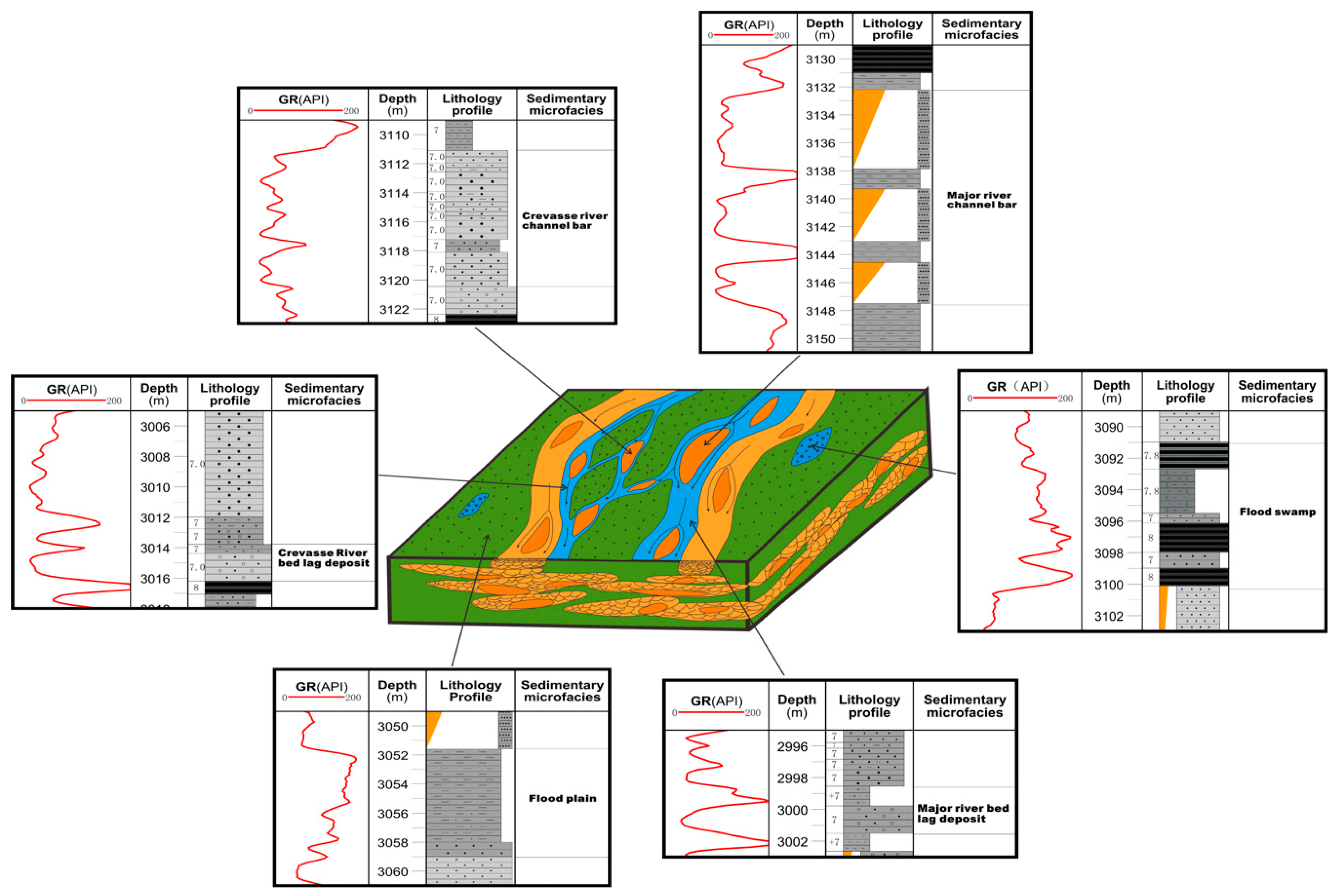
Generally, the sedimentary background of the study area should be known and the qualitative identification model of depositional microfacies should be established [28,29]. The target reservoir in the study area is the He-8 reservoir of Lower Shihezi in the Su-77 block of the Sulige gas field, and the whole body of He-8 is sandy braided river depositional systems in a region of wet marshes, at a certain distance from the sediment provenance [30,31]. The corresponding relationship between the shape and the superimposed pattern of well logs in cored wells and the total of six sedimentary microfacies was established, which is different from those braided river geological models proposed by Miall et al. [32,33]. The river was transformed into a more arid climate from bottom to top as the swing of the river increased. The depositional microfacies models in this area are shown in Figure 1.
Based on the observation of outcrops, drilled cores and thin sections in the study area, combining the identified depositional microfacies with their corresponding log curve shape characteristics, the standard microfacies identification models suitable for the study area are established [34,35,36]. Table 1 shows six types of main microfacies of the braided river in the study area.
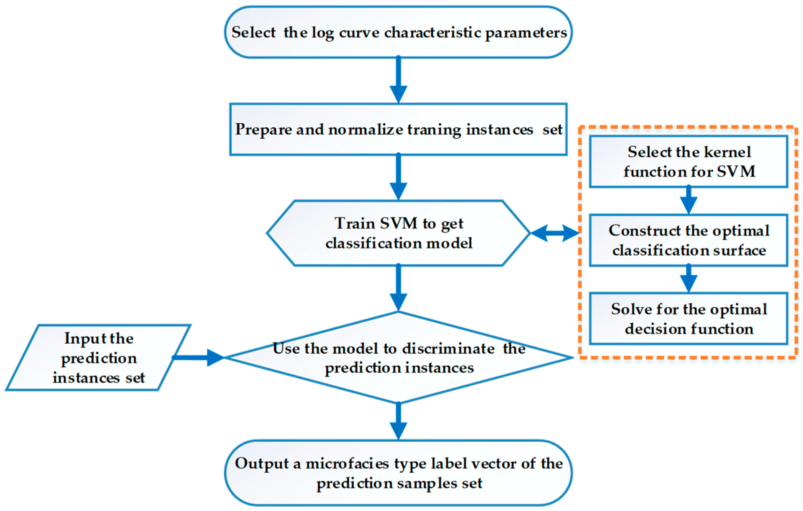
After establishing the qualitative identification models of depositional microfacies in the study case, the quantitative identification of depositional microfacies could then be performed. The key idea of quantitative identification of depositional microfacies by logging data based on the SVM algorithm is that each depositional microfacies can be represented by a set of eigenvectors (log curves characteristic parameters). Sample sets of different microfacies types are mapped to a higher dimension space by nonlinear transformation. This method seeks the optimal classification plane among the samples in the high dimensional feature space, which enables the classification surface to both guarantee the classification accuracy and maximize the interval between two classes of data. Finally, decision functions are constructed to determine the microfacies type of unknown prediction samples as well as the output type labels of the prediction samples, thus achieving depositional microfacies identification [37,38]. The Figure 2 presents the main flow chart of the methodology. The following subsections introduce the steps in details.
2.1. Data Preparation
Data mining and mathematical analysis of the log curves were carried out to determine the characteristic parameters corresponding to the depositional microfacies. After the analysis of the available logs of the study area, the natural gamma curve (GR) [39]—which can best reflect the depositional microfacies of the study area—was selected. The parameters used to quantitatively describe the log curve characteristics were extracted from several aspects such as the curve shape, top–bottom contact relationship and smoothness [3,40]. The value of shale content Vsh is used as a constraint to improve the microfacies identification in the complex geological conditions of the tight sandstone reservoirs in the study area. It is better to extract more characteristic parameters of log curves that can be used to express geological characteristics from density, neutron and acoustic logging curves. The number of characteristic parameters [41,42] in this study that were selected to characterize sedimentary microfacies extracted from well logs was 11; The data were normalized.
The training instances, that is, the matrix (m by n) needs to be constructed. Each column represents a characteristic parameter with a total of n characteristic parameters. Each row represents an instance, with a total of m instances. The training instances are , where m is the number of instances, among which, is the ith instance. The output is , which represents the classification label. If belongs to a certain class, the corresponding output is labeled as ; if it does not belong to a certain class, the output is labeled as . The data sets used in this study were extracted from the well logs of six cored wells in the He-8 reservoir of the Lower Shihezi Formation in Ordos basin, China. The China National Petroleum Corporation (CNPC) provided the petrophysical well logs and corresponding petrographic core analysis reports. The training instances include 11 features parameters as displayed in Table 2.
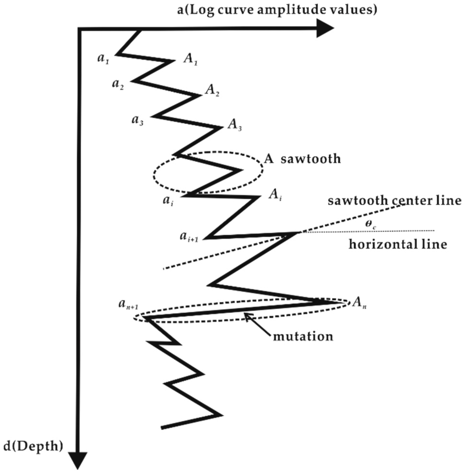
Figure 3 is the schematic diagram describing the shape of a log curve. The log is sampled with a constant sampling interval from top to bottom, and log samples were obtained: depths versus corresponding log reading (amplitude) values . The thickness is calculated as well. Within the determined depth window, using the determined minimum amplitude of gear tooth as the lowest limit, the maximum and minimum values of the amplitude and depth sequence from top to bottom were obtained successively. The extreme value and depth sequence of log curve are obtained. Finally, it is assumed that the sequence started and ended with a valley (see Figure 3). The vertical axis is the depth, and the horizontal axis is the log value. ai is the log reading value, and Ai is the extreme value. The wave peak is found to exhibit a sawtooth form.
The four categories of feature parameters listed in Table 2 represents curve shape (G, S, P, Am), contact relation with top and bottom beds (am-b, am-t, Kp), smoothness (m, R, Kc), and geological constraint parameters (Vsh). The acquisition of these characteristic parameters is an important step in the data preparation stage, and it is also the basis of this method. Previous researchers did not systematically and clearly tell the readers how to acquire these parameters and their meanings. To enable the readers to understand better and reproduce this method, this paper re-combed how these parameters are calculated in the following paragraphs of Section 2.1 and elaborated their geological significance in detail.
The curve shape of the log curve includes feature parameters of G, S, P, and Am. G reflect the curve shape and also explain the graded sequence of the sedimentary rock grains [41]. It can be expressed as:
where G is the relative center of gravity, dimensionless; ai is the ith log value; n is the number of attributes features of the samples. When , the center of gravity is lower and the shape of the curve is bell-shaped, which indicates that the energy of water flow decreases gradually, the supply of sediment provenance decreases gradually and the sedimentary rock grain usually exhibits a graded bed sequence. When , the curve is funnel-shaped and the center of gravity is higher, which reflects the gradual increase of the water flow energy, the gradual increase of the sediment provenance supply and the sedimentary rock grain has a reversed grain sequence. When , the curve shape is a box type—symmetrical or flat tooth-shaped—which represents the abundant supply of sediment provenance in the process of sedimentation, strong hydrodynamic force conditions and a stable sedimentary environment. The S reflects the undulatory property of the curve data [41] and can be expressed as:
where S is the variance of log amplitude, dimensionless; represents the mean values of the n data points; represents the ith log values. n represents the number of sampling points in the selected curve section. S can reflect the physical property of rock to a certain extent. If the grain-size sorting is good, there would be few changes to the physical property, and the log curve shape would be approximately a straight line (mainly a box shape). The log data mean value would be close to most log values over the middle part of the curve, and only a few log values over the top and bottom parts of the curve would be different from the log data mean value. So, S would be smaller. If the grain-size sorting is poor and the physical property variation is significant, the logging curve would have some fluctuation. The curve may be funnel-shaped, bell-shaped or finger-shaped, and the log data would be relatively dispersed. Some of the data points would deviate from the mean value, so S would be bigger. The mean square deviation S can be used to distinguish box shape and other morphology. The P reflect the rate of lithological change [41] and can be expressed as:
where P is the ratio of the amplitude to the thickness of a log curve, dimensionless; indicates the difference between the extreme value of the log curve and the value of the shale baseline; indicates the thickness of the formation (m). As for the sand-shale formations, the larger the value of , the more abundant the sediment source, and the shape of the curve is observed to be box type when the physical property changes little. On the contrary, if the value of is small, this illustrates only a thin interlayer, the deposition time is short and the curve segment shape is finger-shaped. The reflect the concentration degree of the primary amplitude values of the curve [41] and can be expressed as:
where is the median of log values, dimensionless; is the mean value of the curve; is the median value of the curve.
The contact relation between top and bottom beds can be described by the combination of two feature parameters—the mutational amplitude difference [42] and the average slope . can be calculated by Equation (5),
where is the mutational amplitude difference, dimensionless; is the maximum amplitude at the mutation; is the minimum amplitude at the mutation. The average slope [42], for data sequences within the depth window of the log curve , can be expressed as:
where Kp is the average slope of a log curve, dimensionless; , . The contact relation between top and bottom beds can reflect the variation rate of the sediment source supply and water flow energy at the initial and final depositional stages of the sand body. There are two types of contact relations are gradual change and abrupt change. The abrupt change position is the position at which the average slope values of two adjacent curve segments change from positive to negative or from negative to positive, and it tends to indicate scouring (abrupt change at the bottom) or sediment provenance interruption (abrupt change at the top).
The smoothness of the log curve can be indicated by the feature parameters of m, R and Kc. The concave–convex shape of the log curve’s envelope can reflect the change of the water flow energy and depositional rate in the process of sedimentation. The convex, straight-line and concave shapes of the envelope corresponding to the variation of the depositional rate being accelerated, linear or subsided, respectively. The second derivative of a function (curve) can represent the concave and convex characteristics of the curve. So, the concave and convex characteristics of the envelope of the log curve can be obtained by the second derivative m of the envelope [41], which is fitted by the maximum value sequence of the log segment. The envelope is fitted by a parabolic curve using Equation (7),
where D is the function of the log curve’s envelope, dimensionless; m is obtained by performing the second derivative of Equation (7). If , the envelope shape is concave–concave downward stands for accelerated deposition; concave upward means decelerated deposition. If the envelope shape is convex–convex downward indicates accelerated deposition; convex upward represents decelerated deposition. If , the envelope shape is linear, which represent uniform deposition. With the combination of m and , the progradational, reprogradational and aggradational cycles of the sediments can be further distinguished. If , it represents the progradational decelerated type. If , it is the progradational accelerated type. If , it is the reprogradational decelerated type. If , it is the reprogradational accelerated type. For the decrement curve, the concavity and convexity of the envelope are determined by the minimum value sequence using the above method. The number of sawtooth waves of a log curve segment can reflect the intermittence of the deposition process and the stability of the sedimentary environment. A different sequence of log points is constructed first. If the sign of adjacent difference values reverses and the absolute difference between adjacent difference values is higher than a specified value, then it is considered as a sawtooth. So, the number of sign reversals of adjacent difference values in a log segment indicates the number of gear teeth (L). R is a relative sawtooth number of a log curve segment [41], and can be expressed as:
where R is the sawtooth rate, dimensionless; L is the number of sawtooth waves; n is the number of log data points in the log curve segment. The sawtooth center line can be represented by the slope K of the gear tooth centerline or the angle between the sawtooth centerline and the horizontal line [42]. In the depth window, the sequence of data amplitude and depth of the log curve is . Selecting the crest as the maximum value and the trough as the minimum value, the sequence of maximum value and depth is , and the sequence of minimum value and depth is . The angle between the tooth center line of the ith crest and the horizontal line can be expressed as:
where is the angle between the tooth center line of the trough and the horizontal line (°). The angle between the tooth center line of the ith trough and the horizontal line [42] can be expressed as:
where is the angle between the tooth center line of the trough and the horizontal line (°). The slope of the tooth centerline [42] of the ith crest can be expressed as:
where is the slope of the tooth centerline of the crest. The slope of the tooth centerline [42] of the ith trough can be expressed as:
where is the slope of the tooth centerline of the trough. and may be used together. In practice, usually one of them (for example, ), is used. If and its value increases from bottom to top, it represents outward convergence and indicates that the deposition rate increases from bottom to top. If and its value decreases from bottom to top, it represents inward convergence and indicates that the deposition rate decreases from bottom to top. If , this indicates that the physical property of the layers is stable, and that the sedimentary environment and sediment provenance are stable. When the value swings seriously, it shows that the sedimentary environment frequently changes, hence causing great changes in the physical property.
The shale content (Vsh) can reflect the magnitude of the flow energy and the distance from the sediment provenance. The shale content of different depositional facies is different and set apart from the changes in the log curve shape. Therefore, the shale content, as a geological constraint parameter, can be used to optimize the microfacies quantitative identification model. The shale content is calculated by the combination of the gamma-ray log and the difference between density porosity and neutron porosity logs.
2.2. SVM Classification Model
The following is the specific process of training the SVM classifier by the training sample set to gain the classification model (optimal decision function), including three steps: selecting the kernel function; constructing the optimal classification surface; solving the optimal decision function [43,44].
2.2.1. Kernel Function
If the low dimensional space is linearly inseparable, it may become linearly separable after being mapped to a higher dimensional feature space through nonlinear mapping. If this technique is used for classification or regression in high dimensional space directly, there will be some challenging issues such as determining the form and parameters of a nonlinear mapping function and the number of dimensions of the feature space.
Support vector machine is used to solve the inner product operation in the high dimensional feature space by using the kernel function in the low dimensional space and avoiding the dimension disaster [45]. The kernel function value is the similarity between and . There are three kinds of kernel functions in SVM, and selecting the suitable kernel function is the key to successful nonlinear classification [46]. In the case of an unknown probability of classification, this paper selects the widely used radial basis function (RBF), which is expressed by Equation (13),
where K is the kernel function; r is the RBF parameter; represents the feature vectors of the training samples; represents the prediction samples. Based on the training samples of depositional microfacies of six cored wells and 11 feature parameters, using the cross-validation method, the obtained optimal kernel function parameter r for identifying positional microfacies in the study case was found to be 0.1.
2.2.2. Optimal Classification Surface
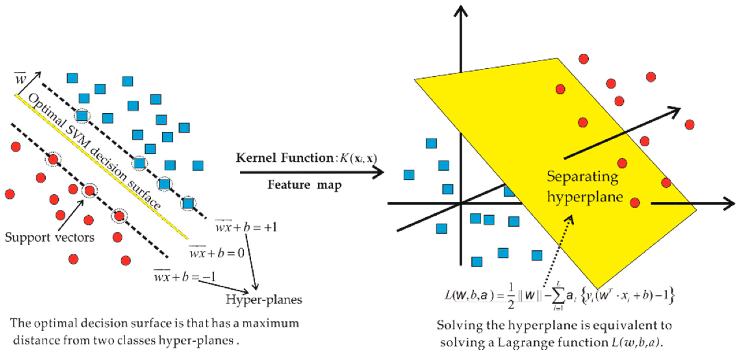
After the input sample is transformed into the high dimensional space using the radial basis kernel function, the optimal classification surface needs to be determined in the high dimensional space (see Figure 4) The separation between different clusters is termed as the hyperplane, and its geometry can be linear, polynomial or radial [25]. w is the normal vector of the optimal SVM decision surface in Figure 4. The red and blue dots in Figure 4 are the features of two different sedimentary microfacies samples. Solving the hyperplane is equivalent to solving a Lagrange function . Nonlinear data set separation is achieved by a separating the hyperplane using a kernel function in the feature space.
After obtaining the optimal classification hyperplane, it can be used to predict the prediction sample set. The determination of the optimal classification surface can be expressed as a constrained optimization based on the Lagrange relaxation method . The optimal objective function of the generalized optimal classification surface of SVM [22] can be transformed into Equation (14),
The corresponding constraint is
where , are the log curve characteristic parameter vectors; , are the microfacies type label vectors of the training samples; c is the penalty parameter. When , the best result of depositional microfacies identification in the study area was achieved. The optimal solution is obtained, then select as a positive component of and calculate , where is the threshold value for classification and is the Lagrange multiplier.
2.2.3. Optimal Decision Function
After the above step, the optimal decision function [21] (expressed by Equation (15)) satisfying the constraint is obtained by solving the optimal classification surface (a quadratic programming optimization problem under the inequality constraint and having a unique solution). The optimal decision function is the categorization model. That is, Model = svmtrain (train_label, train_matrix, [option]).
where denotes the feature vectors of the training samples; represents the prediction samples; and are output depositional microfacies types labels of the training samples and prediction samples, respectively; is the kernel function; is the number of samples.
2.3. Discrimination of the Prediction Instances
After obtaining the classification model by the training samples, the model was used to discriminate the depositional microfacies types of prediction samples. Finally, the microfacies type label column vector of the prediction samples are the output, and the row number of the column vector is equal to the number of the prediction sample set matrix. That is, [predict_label, accuracy] = svmpredict (predict_label, predict_matrix, model).
Finally, the “one against one” method was used to perform multi-classification [22]. Any two sample sequences were combined to construct vector machines, the "vote" was adopted to classify and perform the identification of N types of depositional microfacies in the intervals without the core.
3. Results and Discussion
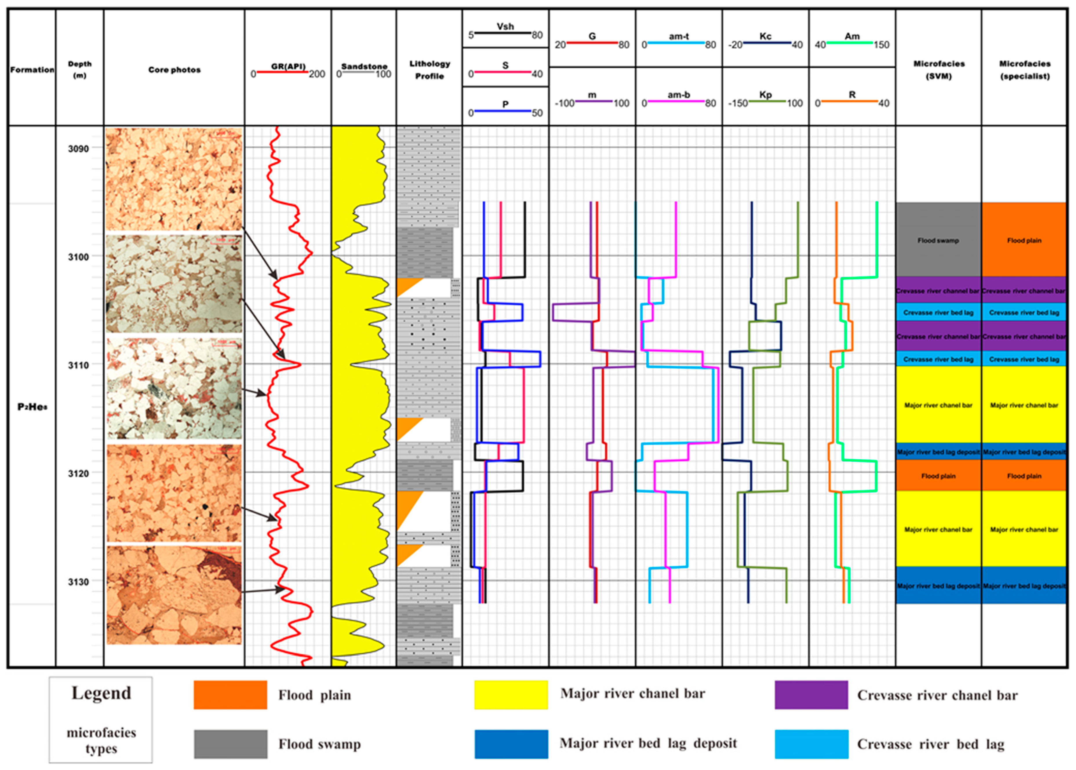
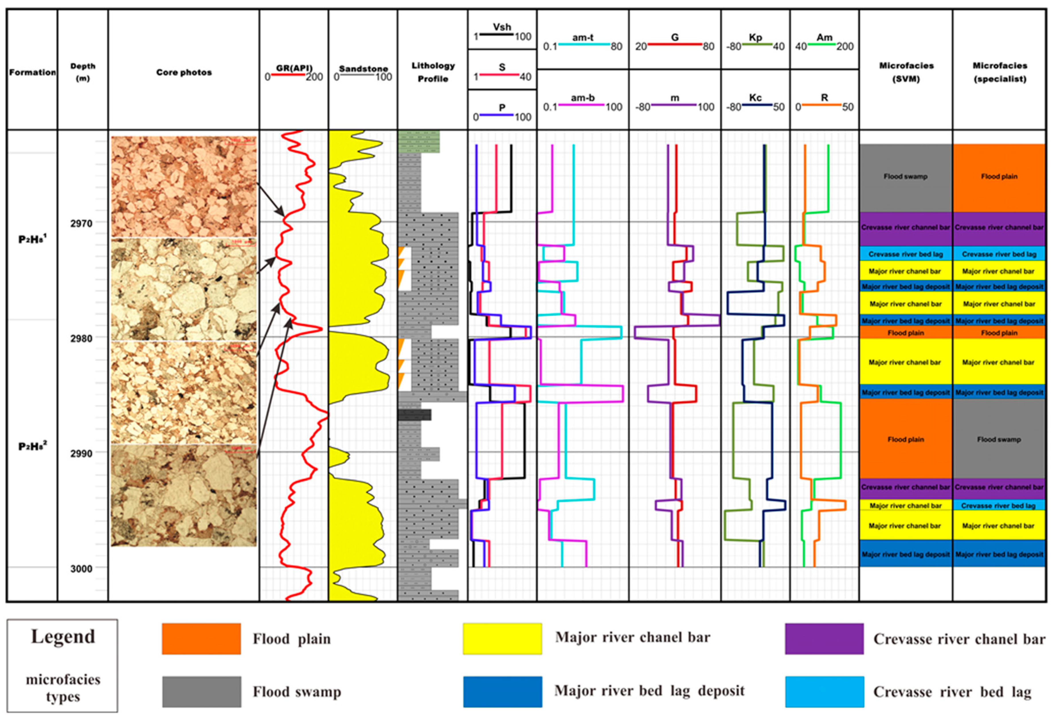
The method proposed in this paper for the automatic identification of microfacies was applied to the H-8 reservoir in multiple wells of the studied area. To verify the results of the method, two cored wells (S77-23-37 and S77-3-21) are randomly selected as verification wells. These two cored wells are not used in the stage of establishing qualitative identification models of depositional microfacies, so they could be used to verify whether the method works or not. In these two verification wells, 25 microfacies including 6 major river bed lag deposit, 4 crevasse river bed lag deposit, 6 major river channel bar, 4 crevasse river channel bar, 1 flood swamp, and 3 flood plain as shown in Table 3 are selected. These 25 depositional microfacies are identified by geologists through the observation of thin slice photographs of core samples and can be regarded as the standard and true depositional microfacies. After the microfacies identification by geologists, these 25 depositional microfacies are processed by the SVM method. To verify the reliability, the identification results by SVM are compared with that by geologists. The comparison results in Figure 5 and Figure 6 show that only 4 layers identified by the SVM are not inconsistent with the results by geologists. In other words, there are 21 accurate recognition results and four errors, so the accuracy rate is 84%.
This paper compares the recognition results between the SVM method and the traditional manual method by a geologist in the two example wells, as shown in Figure 5 and Figure 6. Some core thin section photos are shown to verify the real results as well. In well S77-3-21 (Figure 6), braided river channel lag deposit and diara deposit occur alternately from 2970 to 2980 m, while the lithology is transitional and the sedimentary thickness is thin. This SVM method accurately identified and distinguished the thin layer, and showed that the automatic method for the identification of depositional microfacies works well in a tight sandstone gas reservoir.
4. Conclusions
In this study, the SVM algorithm is introduced and applied to automatically identify depositional microfacies using well logs. The following conclusions have been obtained. (1) The comprehensive, accurate, and quantitative description of the variation characteristics of log curves is the foundation for the automatic identification of depositional microfacies by SVM algorithm. That is, four categories of feature parameters in terms of curve shape, contact relation with top and bottom beds, smoothness, and geological constraint parameters should be used as the input parameters of SVM. (2) The SVM follows the steps of selecting radial basis function, obtaining the SVM discrimination model of depositional microfacies by training sample sets, and realizing the discrimination of predicted samples. (3) The application of SVM in the He-8 reservoir of Lower Shihezi in the Su-77 block of the Sulige gas field shows that the SVM algorithm can automatically and quantitatively identify depositional microfacies with a rate of accuracy approaching 84%.
In summary, this study proposes an innovative and constructive solution for identifying depositional microfacies. This innovative and constructive solution for identifying depositional microfacies will contribute to the cost-saving of core analysis and improve the sustainable profitability of oil and gas exploration. However, the application of this method needs to take into consideration the regional sedimentary environment and the geological stratification. Future work to improve this method will focus on the combination of automatic stratification technology, signal analysis technology and the selection of microfacies-sensitive log curves. This method in our study was only applied in the depositional microfacies identification of tight sandstone gas reservoirs. It has potential applications in carbonate and shale reservoirs, although the universal applicability of the method in these two kinds of reservoirs should be verified.
Author Contributions
Conceptualization, J.P.; Writing—original draft, D.W.; Methodology, Q.Y.; Data curation, Y.C.; Writing—review and editing, H.Y.
Funding
This research was funded by the National Science and Technology Major Project of China (Grant no. 2016ZX05052) and the National Natural Science Foundation of China (Grant Nos. 41504108 and 41872166).
Acknowledgments
The authors thank Wang Liang and Sima Liqiang of Southwest Petroleum University for their constructive help.
Conflicts of Interest
The authors declare no conflict of interest.
References
- Pirson, S.J. Handbook of Well Log Analysis for Oil and Gas Formation Evaluation; Schlumberger Limited: Houston, TX, USA, 1963. [Google Scholar]
- Serra, O.; du Pétrole, I.F. Well Logging and Reservoir Evaluation; Technip: Paris, France, 2007. [Google Scholar]
- Serra, O.; Serra, L. Well Logging and Geology; Serralog: Caxias do Sul, Brazil, 2003. [Google Scholar]
- Serra, O.; Serra, L. Well Logging: Data Acquisition and Applications; Serralog: Méry Corbon, France, 2004. [Google Scholar]
- Wang, L.; Fu, Y.; Li, J.; Sima, L.; Wu, Q.; Jin, W.; Wang, T. Mineral and pore structure characteristics of gas shale in Longmaxi formation: A case study of Jiaoshiba gas field in the southern Sichuan Basin, China. Arab. J. Geosci. 2016, 9, 733. [Google Scholar] [CrossRef]
- Wang, L.; Yin, R.; Sima, L.; Fan, L.; Wang, H.; Yang, Q.Q.; Huang, L.L. Insights into Pore Types and Wettability of a Shale Gas Reservoir by Nuclear Magnetic Resonance: Longmaxi Formation, Sichuan Basin, China. Energy Fuels 2018, 32, 9289–9303. [Google Scholar] [CrossRef]
- Wang, L.; Zhao, N.; Sima, L.; Meng, F.; Guo, Y.H. Pore structure characterization of the tight reservoir: Systematic integration of mercury injection and nuclear magnetic resonance. Energy Fuels 2018, 32, 7471–7484. [Google Scholar] [CrossRef]
- Donselaar, M.E.; Schmidt, J.M. Integration of outcrop and borehole image logs for high–resolution facies interpretation: Example from a fluvial fan in the Ebro Basin, Spain. Sedimentology 2005, 52, 1021–1042. [Google Scholar] [CrossRef]
- Kadkhodaie, A.; Rezaee, R. Intelligent sequence stratigraphy through a wavelet-based decomposition of well log data. J. Nat. Gas Sci. Eng. 2017, 40, 38–50. [Google Scholar] [CrossRef]
- Lai, J.; Wang, G.W.; Fan, Z.Y.; Chen, J.; Wang, S.C.; Fan, X. Q, Sedimentary characterization of a braided delta using well logs: The Upper Triassic Xujiahe Formation in Central Sichuan Basin, China. J. Pet. Sci. Eng. 2017, 154, 172–193. [Google Scholar] [CrossRef]
- Li, W.B.; Yu, Y.L.; Wang, J.Q.; Bai, Y.; Wang, X. In Application of Self-Organizing Neural Network Method in Logging Sedimentary Microfacies Identification. In Advanced Materials Research; Trans Tech Publications: Zurich Switzerland, 2013; pp. 38–42. [Google Scholar] [CrossRef]
- Sebtosheikh, M.A.; Motafakkerfard, R.; Riahi, M.A.; Moradi, S.; Sabety, N. Support vector machine method, a new technique for lithology prediction in an Iranian heterogeneous carbonate reservoir using petrophysical well logs. Carbonates Evaporites 2015, 30, 59–68. [Google Scholar] [CrossRef]
- Zhang, F.; Li, H. Application of artificial neural network pattern recognition technology to the study of well-logging sedimentology. Pet. Explor. Dev. 2003, 30, 121–123. [Google Scholar] [CrossRef]
- Zhang, J.; Liu, S.; Li, J.; Liu, L.; Liu, H.; Sun, Z. Identification of sedimentary facies with well logs: An indirect approach with multinomial logistic regression and artificial neural network. Arab. J. Geosci. 2017, 10, 1–9. [Google Scholar] [CrossRef]
- Mohri, M.; Rostamizadeh, A.; Talwalkar, A. Foundations of Machine Learning; MIT Press: Cambridge, MA, USA, 2018. [Google Scholar]
- Atluri, G.; Karpatne, A.; Kumar, V. Spatio-temporal data mining: A survey of problems and methods. ACM Comput. Surv. 2018, 51, 83. [Google Scholar] [CrossRef]
- Jordan, M.I.; Mitchell, T.M. Machine learning: Trends, perspectives, and prospects. Science 2015, 349, 255–260. [Google Scholar] [CrossRef] [PubMed]
- Berry, D.A.; Stangl, D. Bayesian Biostatistics; CRC Press: Boca Raton, FL, USA, 2018. [Google Scholar] [CrossRef]
- Chaghari, A.; Feizi-Derakhshi, M.; Balafar, M. Fuzzy clustering based on Forest optimization algorithm. J. King Saud Univ. Comput. Inf. Sci. 2018, 30, 25–32. [Google Scholar] [CrossRef] [Green Version]
- Van Gerven, M.; Bohte, S. Artificial Neural Networks as Models of Neural Information Processing; Frontiers Media SA: Lausanne, Switzerland, 2018. [Google Scholar] [CrossRef]
- Vapnik, V. The Nature of Statistical Learning Theory; Springer Science & Business Media: Berlin/Heidelberg, Germany, 2013. [Google Scholar] [CrossRef]
- Krebel, U. Pairwise classification and support vector machines. In Advances in Kernel Methods: Support Vector Learning; MIT Press: Cambridge, MA, USA, 1999; pp. 255–268. [Google Scholar]
- Thanh Noi, P.; Kappas, M. Comparison of random forest, k-nearest neighbor, and support vector machine classifiers for land cover classification using Sentinel-2 imagery. Sensors 2018, 18, 18. [Google Scholar] [CrossRef] [PubMed]
- Gharagheizi, F.; Mohammadi, A.H.; Arabloo, M.; Shokrollahi, A. Prediction of sand production onset in petroleum reservoirs using a reliable classification approach. Petroleum 2017, 3, 280–285. [Google Scholar] [CrossRef] [Green Version]
- Palaniswami, M.; Shilton, A.; Ralph, D.; Owen, B.D. Machine learning using support vector machines. In Proceedings of the International Conference on Artificial Intelligence in Science and Technology, Hobart, Australia, 9–12 February 2000. [Google Scholar]
- Chang, C.C.; Lin, C.J. LIBSVM: A library for support vector machines. ACM Trans. Intell. Syst. Technol. 2011, 2, 27. [Google Scholar] [CrossRef]
- Jones, H. Machine Learning: An Essential Guide to Machine Learning for Beginners Who Want to Understand Applications, Artificial Intelligence, Data Mining, Big Data and More; CreateSpace Independent Publishing Platform: Scotts Valley, CA, USA, 2018. [Google Scholar]
- Nichols, G. Sedimentology and Stratigraphy; John Wiley & Sons: Hoboken, NJ, USA, 2009. [Google Scholar]
- Reading, H.G. Sedimentary Environments: Processes, Facies and Stratigraphy; John Wiley & Sons: Hoboken, NJ, USA, 1996. [Google Scholar]
- Fan, E.P.; Cheng, Y.H.; Zhang, Y.Z.; Bai, Z.H. Sedimentology and Reservoir Characteristics of He8 Member, in a Gas Field of Ordos Basin, Northern China. In Advanced Materials Research; Trans Tech Publications: Zurich Switzerland, 2013; pp. 161–165. [Google Scholar] [CrossRef]
- Li, Y.J.; Zhao, Y.; Yang, R.C.; Fan, A.P.; Li, F.P. Detailed sedimentary facies of a sandstone reservoir in the eastern zone of the Sulige gas field, Ordos Basin. Min. Sci. Technol. (China) 2010, 20, 891–903. [Google Scholar] [CrossRef]
- Miall, A.D. The Geology of Fluvial Deposits: Sedimentary Facies, Basin Analysis, and Petroleum Geology; Springer: Berlin/Heidelberg, Germany, 1996. [Google Scholar] [CrossRef]
- Bridge, J.S.; Lunt, I.A. Depositional models of braided rivers. Braided Rivers Process. Ecol. Manag. 2006, 36, 11–50. [Google Scholar] [CrossRef]
- Medici, G.; Boulesteix, K.; Mountney, N.P.; West, L.J.; Odling, N.E. Palaeoenvironment of braided fluvial systems in different tectonic realms of the Triassic Sherwood Sandstone Group, UK. Sediment. Geol. 2015, 329, 188–210. [Google Scholar] [CrossRef] [Green Version]
- Skelly, R.L.; Bristow, C.S.; Ethridge, F.G. Architecture of channel-belt deposits in an aggrading shallow sandbed braided river: The lower Niobrara River, northeast Nebraska. Sediment. Geol. 2003, 158, 249–270. [Google Scholar] [CrossRef]
- Hjellbakk, A. Facies and fluvial architecture of a high-energy braided river: The Upper Proterozoic Seglodden Member, Varanger Peninsula, northern Norway. Sediment. Geol. 1997, 114, 131–141, 145–149, 153–161. [Google Scholar] [CrossRef]
- Gupta, I.; Rai, C.S.; Sondergeld, C.H.; Devegowda, D. Rock Typing in Eagle Ford, Barnett, and Woodford Formations. SPE Reserv. Eval. Eng. 2018. [Google Scholar] [CrossRef]
- Bolandi, V.; Kadkhodaie, A.; Farzi, R. Analyzing organic richness of source rocks from well log data by using SVM and ANN classifiers: A case study from the Kazhdumi formation, the Persian Gulf basin, offshore Iran. J. Pet. Sci. Eng. 2017, 151, 224–234. [Google Scholar] [CrossRef]
- Nazeer, A.; Abbasi, S.A.; Solangi, S.H. Sedimentary facies interpretation of Gamma Ray (GR) log as basic well logs in Central and Lower Indus Basin of Pakistan. Geod. Geodyn. 2016, 7, 432–443. [Google Scholar] [CrossRef] [Green Version]
- Serra, O. Sedimentary Environments from Wireline Logs; Schlumberger Limited: Houston, TX, USA, 1985. [Google Scholar]
- Liu, H.Q.; Chen, P.; Xia, H.Q. Automatic identification of sedimentary microfacies with log data and its application. Well Logging Technol. 2006, 30, 233. [Google Scholar] [CrossRef]
- Ma, S.Z.; Huang, X.O.; Zhang, T.B. Mathematic method for quantitative automatic identification of logging microfacies. Oil Geophys. Prospect. 2000, 35, 582–589. [Google Scholar] [CrossRef]
- Chang, C.C.; Lin, C.J. LIBSVM: A library for support vector machines. ACM Trans. Intell. Syst. Technol. (TIST) 2011, 2, 27. [Google Scholar] [CrossRef]
- Burges, C.J.C. A tutorial on support vector machines for pattern recognition. Data Min. Knowl. Discov. 1998, 2, 121–167. [Google Scholar] [CrossRef]
- Cristianini, N.; Shawe-Taylor, J. An Introduction to Support Vector Machines and Other Kernel-Based Learning Methods. Kybernetes 2001, 32, 1–28. [Google Scholar] [CrossRef]
- Brereton, R.G.; Lloyd, G.R. Support vector machines for classification and regression. Analyst 2010, 135, 230–267. [Google Scholar] [CrossRef] [PubMed]
Figure 1.
Braided river depositional microfacies qualitative identification models of the He-8 reservoir of the Su-77 block in the Sulige gas field, Ordos basin.
Figure 1.
Braided river depositional microfacies qualitative identification models of the He-8 reservoir of the Su-77 block in the Sulige gas field, Ordos basin.

Figure 2.
Flow chart of depositional microfacies classification method by support vector machine (SVM).
Figure 2.
Flow chart of depositional microfacies classification method by support vector machine (SVM).

Figure 3.
Schematic diagram of well logging curve shape modified from Ma et al. [42].
Figure 3.
Schematic diagram of well logging curve shape modified from Ma et al. [42].

Figure 4.
Schematic diagram of the optimal classification, support vectors, hyperplane, and optimal SVM decision surface.
Figure 4.
Schematic diagram of the optimal classification, support vectors, hyperplane, and optimal SVM decision surface.

Figure 5.
Comparison of the microfacies identification results by SVM method and geologists in well S77-23-37.
Figure 5.
Comparison of the microfacies identification results by SVM method and geologists in well S77-23-37.

Figure 6.
Comparison of the microfacies identification results by SVM method and geologists in well S77-3-21.
Figure 6.
Comparison of the microfacies identification results by SVM method and geologists in well S77-3-21.


Table 1.
Braided river depositional microfacies types of the He-8 reservoir of the Su-77 block in the Sulige gas field.
Table 1.
Braided river depositional microfacies types of the He-8 reservoir of the Su-77 block in the Sulige gas field.
| Depositional Facies | Subfacies | Microfacies | |
|---|---|---|---|
| Braided river | River channel | River bed lag deposit | Major river bed lag deposit |
| Crevasse river bed lag deposit | |||
| Diara | Major river channel bar | ||
| Crevasse river channel bar | |||
| Fluviatile flood plain | Flood swamp | ||
| Flood plain | |||
Table 2.
Characteristic parameters of log curves and corresponding depositional microfacies in the study area.
Table 2.
Characteristic parameters of log curves and corresponding depositional microfacies in the study area.
| Depositional Microfacies | Curve Shape | Contact Relation with Top and Bottom Beds | Smoothness | Geological Constraint | |||||||
|---|---|---|---|---|---|---|---|---|---|---|---|
| G × 102 | S | P | Am | am-b | am-t | Kp × 103 | m | R × 102 | Kc × 104 | Vsh | |
| Major river channel bar | 51.9 | 67.32 | 32 | 80.56 | 160 | 140 | 4.1 | −0.6 | 99 | 2.07 | 3.2 |
| Crevasse river channel bar | 48.9 | 16.66 | 5 | 56.96 | 44 | 77 | −41.5 | 0.48 | 11 | 5.75 | 20.16 |
| Major river bed lag deposit | 49 | 49.42 | 13 | 81.68 | 100 | 86 | −5.3 | −2.02 | 10 | −0.45 | 25.1 |
| Crevasse river bed lag deposit | 47.5 | 27.29 | 25 | 58.9 | 140 | 100 | −12 | 5.84 | 8 | 13.48 | 25.06 |
| Flood plain | 53.6 | 23.08 | 6 | 136.76 | 120 | 20 | 70.7 | −0.46 | 14.1 | 1.27 | 31.83 |
| Flood swamp | 49.1 | 23.28 | 11 | 138.55 | 100 | 50 | −31.4 | −2.86 | 23 | 1.28 | 69.2 |
Table 3.
Comparison of the microfacies identification results by SVM method and geologists.
| Methods | Depositional Microfacies | |||||
|---|---|---|---|---|---|---|
| Major River Bed Lag Deposit | Crevasse River Bed Lag Deposit | Major River Channel Bar | Crevasse River Channel Bar | Flood Swamp | Flood Plain | |
| SVM | 6 | 3 | 7 | 4 | 2 | 3 |
| Geologist | 6 | 4 | 6 | 4 | 1 | 3 |
© 2019 by the authors. Licensee MDPI, Basel, Switzerland. This article is an open access article distributed under the terms and conditions of the Creative Commons Attribution (CC BY) license (http://creativecommons.org/licenses/by/4.0/).
Share and Cite
MDPI and ACS Style
Wang, D.; Peng, J.; Yu, Q.; Chen, Y.; Yu, H. Support Vector Machine Algorithm for Automatically Identifying Depositional Microfacies Using Well Logs. Sustainability 2019, 11, 1919. https://0-doi-org.brum.beds.ac.uk/10.3390/su11071919
AMA Style
Wang D, Peng J, Yu Q, Chen Y, Yu H. Support Vector Machine Algorithm for Automatically Identifying Depositional Microfacies Using Well Logs. Sustainability. 2019; 11(7):1919. https://0-doi-org.brum.beds.ac.uk/10.3390/su11071919
Chicago/Turabian StyleWang, Dahai, Jun Peng, Qian Yu, Yuanyuan Chen, and Hanghang Yu. 2019. "Support Vector Machine Algorithm for Automatically Identifying Depositional Microfacies Using Well Logs" Sustainability 11, no. 7: 1919. https://0-doi-org.brum.beds.ac.uk/10.3390/su11071919
Note that from the first issue of 2016, this journal uses article numbers instead of page numbers. See further details here.