Environmental Efficiency Measurement and Convergence Analysis of Interprovincial Road Transport in China

Abstract

Although road transport plays a vital role in promoting the development of China’s national economy, it also produces much harmful output in the process of road transport. Various types of harmful output generate high social costs. In order to improve efficiency and protect the environment at the same time, a variety of undesirable outputs need to be considered when evaluating the environmental efficiency of road transport. In this paper, the performance of the road transport systems in 30 regions of China is evaluated considering multiple harmful outputs (noise, carbon emission, direct property losses), by employing the directional distance function. Further, a convergence analysis of the environmental efficiency of road transport is carried out. The empirical results show that the environmental efficiency of overall road transport in China increased from 0.8851 to 0.9633 from 2010 to 2017. Moreover, the environmental efficiency gaps between the eastern, central and western areas have narrowed over time, but still exist. Additionally, the results of σ convergence analysis show that convergence of environmental efficiency exists in the whole country and the western area, while only weak convergence exists in the eastern and central areas. Both absolute β convergence and conditional β convergence exist in the eastern, central and western areas. While the environmental efficiency improved over the study period, the environmental efficiencies of road transport in some provinces remain inefficient, which deserves more attention from those seeking to improve environmental efficiency. The paper concludes with suggestions for improving the environmental efficiency of road transport.

1. Introduction

Road transport is an indispensable part of China’s comprehensive transport system and plays a crucial role in promoting regional economic development and logistics operation [1,2]. In recent years, with the government’s emphasis on road transport and the development of social economy, the investment of relevant departments in road construction has increased significantly. By the end of November 2019, China’s fixed-asset investment in roads reached 2024.214 billion yuan, up 1.9% from the same period in 2018 [3]. With the steady growth of market investment, the highway mileage of China’s road transport is also increasing every year. The length of China’s road transport reached 4.8465 million kilometers in 2018, an increase of 73,000 km compared with 2017 [4]. At present, China’s road freight market still occupies the largest proportion in the whole freight market. By November 2019, China’s freight volume had reached 486.31 million tons, with China’s road freight volume the largest, at 77.81 percent [3].

While road transport has made brilliant achievements, it will also face a series of negative problems caused by its success. Road transport not only produces air pollution but also emits greenhouse gases that contribute to global warming [5]. From 2009 to 2012, the average annual emission of carbon dioxide from the road transport sector in China reached 529.31 million tons [6]. Moreover, traffic accidents are a leading cause of casualties and property damage [7]. From 2010 to 2017, the direct property loss caused by traffic accidents increased from 0.92 billion to 1.21 billion, and the average direct property loss during this period reached 1.09 billion [3]. The average noise level in road transport is 69 dB, which is higher than the environmental noise standard and constitutes another environmental issue [4]. These environmental and safety issues do affect the performance and long-term development of the road transport sector, perhaps so much that it cannot maintain its competitive advantage in integrated transport systems. Therefore, it is necessary to assess the environmental efficiency, considering the environmental and safety problems caused by road transport, so as to provide managers and decision makers with a basis for planning and action.

Many studies omit consideration of multiple undesirable outputs, and various undesirable outputs, such as traffic accidents and noise, are easily ignored. Therefore, this paper selects carbon dioxide emission, noise and direct property loss caused by traffic accidents as the undesirable outputs to evaluate, along with the traditional efficiency evaluation index. The directional distance function (DDF), which takes into account both good and harmful outputs, is used to assess the environmental efficiency of the road transport. On this basis, the convergence of environmental efficiency is tested.

The purpose of this paper is to measure the environmental efficiency of China’s road transport by considering a variety of undesirable outputs, and to analyze whether the environmental efficiency has reached a stable level. There are two main contributions of this paper. As for the method, data envelopment analysis with the DDF is used to evaluate the performance of road transport departments; using this technique, both good and bad output are considered, and the convergence of the environmental efficiency can be tested. As for the variable selection, we choose carbon dioxide emission, direct property loss caused by traffic accidents and noise as the indicators of undesirable output. The models of most of the existing literature use carbon dioxide emission or traffic accidents as the single undesirable output, and a few publications consider traffic noise.

Next, Section 2 reviews the literature on transport environmental efficiency. Section 3 introduces the DDF, data envelopment analysis (DEA), and the method of convergence analysis in the study of environmental efficiency. Section 4 describes input-output indicators and data related to road transport, as well as empirical results. Finally, the paper offers implications and highlights its main conclusions. Appendix A is a Table of notation used in this study (

Table A1. Table of Notation.

Symbols	Descriptions	Symbols	Descriptions
DEA	Data Envelopment Analysis	OLS	Ordinary Least Squares
DDF	Directional distance function	dB	Decibel
SFA	Stochastic Frontier Analysis	PM2.5	Fine particulate matter
CE	Carbon dioxide emission	$y^d$	Desirable output
SBM	Slack Based Measure	$y^u$	Undesirable output
$S{D}_t$	Standard Deviation	$\epsilon$	Random error
$CC{F}_i$	Carbon content factor	$E{F}_{i,t}$	Road transport efficiency
$CO{F}_i$	Hydrocarbon coefficient	$A_i$	Energy consumption
$H{E}_i$	Equivalent thermal	$g_{y^d}$	The direction vector of desirable output
GDP	Gross Domestic Product	$g_{y^u}$	The direction vector of undesirable output

).

2. Literature Review

2.1. A Review of Road Transport Efficiency Ignoring Environmental Factors

The existing literature contains both parametric methods and nonparametric methods to measure road transport efficiency, represented by stochastic frontier analysis (SFA) and DEA, respectively. DEA is a mature efficiency evaluation method which does not need any specific production function form and has been widely used in the evaluation of transport efficiency [8]. Earlier, many scholars used DEA to study transport efficiency. Karlaftis [9] used DEA to estimate the efficiency of 256 transport systems in the United States. Jain et al. [10] employed a DEA method to analyze the efficiency of an urban transit rail transport system, pointing out that privatization is conducive to the improvement of transport efficiency. Yu and Fan [11] proposed a mixed structure network DEA to measure the technical efficiency of Taiwan’s public transport system. Kumar [12] used traditional DEA and a super-efficiency model to measure road transport efficiency, and Tobit analysis was used to explain the factors affecting that efficiency. Yang et al. [13] evaluated urban road transport with a hybrid DEA model. From the research of these scholars, it can be found that their DEA models only consider good output, ignore bad output, and do not conform to the actual production process.

Other scholars use the parametric method SFA to evaluate transport efficiency. For example, Holmgren and Johan [14] employed SFA as a tool for analyzing how the efficiency of public transport operations in 26 Swedish counties changes over time. Jarboui et al. [15] used SFA to comprehensively analyze the technical efficiency of 54 public road transport operators in 18 countries. Ayadi and Hammami [16] used the SFA method to evaluate the efficiency of 12 Tunisian bus transport companies during the 2000–2010 period. SFA requires choosing an appropriate form of the production function, and its model hypothesis is relatively complex, which brings difficulties to empirical research. For this reason, many researchers prefer to use DEA to measure efficiency [17]. If the SFA production function form is not selected correctly, then the skewness problem easily appears and the final calculation result is not credible [18].

2.2. A Review of Road Transport Efficiency Considering Environmental Factors

Governments are paying increasing attention to the escalating issues involving environmental deterioration [19]. Accordingly, many studies also focus on environmental performance when considering efficiency, and many scholars have suggested that the impact of environmental factors on transport efficiency should be considered [20,21,22,23]. Zhou et al. [24] used the output-oriented directional distance function to measure the performance of China’s transport sector, considering CO₂ emissions as adverse output. Agarwal et al. [25] took traffic accidents as input variables and used DEA to measure the efficiency of the traffic sector in India. Liu et al. [26] selected CO₂ emissions as the only undesirable output, and the non-radial DEA model was used to measure the environmental efficiency of road and rail transport in 30 regions of China. Liu et al. [6] proposed a parallel DEA method based on slacks, to evaluate the environmental efficiency of railway and road transport and the comprehensive efficiency of both, considering carbon dioxide emissions.

Pal and Mitra [27] adopted traffic accidents as the undesirable output, measured the performance of 37 road transport enterprises by using the DDF, and studied the factors causing traffic accidents by using the Tobit model. Park et al. [28] employed slack-based DEA to measure environmental efficiency in the American transport sector, taking CO₂ emissions into account as a bad output. In addition, the carbon efficiency and potential emission reductions of the 50 states were estimated. Wu et al. [29] proposed an extended parallel DEA method to measure and compare the environmental efficiency of passenger and freight for China’s road transport, taking into account CO₂ emissions. Wang [5] used the SBM-DEA model to evaluate the environmental efficiency of road transport, considering the total number of accidental casualties due to traffic accidents, CO₂ emissions, and PM2.5 as harmful outputs. Piccioni [30] implemented a set of transport, cost and investment sub-models applied in series. In such a context, road efficiency is linked to some parameters, such as maintenance costs (mileage) and additional costs that compensate for the major negative externalities (environmental problems, traffic jam) of road traffic. Wang et al. [31] predicted CO₂ emissions from road freight in China in different situations, by employing system optimization. Omrani et al. [32] used a comprehensive DEA model to analyze the energy efficiency of Iran’s road transport sector, incorporating CO₂ emissions into the model as the only environmental factor.

In the literature considering environmental factors, scholars have two ways of dealing with harmful outputs. One takes them as inputs and assumes that the harmful outputs are freely disposable [33,34]. The other treats them as outputs, supposing that they have weak disposability. However, the former method is controversial for two reasons: first, considering the undesirable output as input is contrary to the actual production process [17]; second, this method does not conform to the “null-jointness” principle of undesirable outputs and desirable output. As for the transport efficiency, many scholars only consider a single undesirable output such as CO₂ emissions or traffic accidents; only rarely does any work consider multiple undesirable outputs. However, the environmental problem encompasses not only the atmospheric pollution caused by CO₂ emissions, but also factors such as the troubles caused by traffic noise. To sum up, we use the DDF model to assess the environmental efficiency of road transport, considering both good output and three types of harmful output: CO₂ emissions, noise and direct property loss caused by traffic accidents. Then, convergence analysis is used to examine whether there is convergence in the environmental efficiency of road transport.

3. Methodology

3.1. The DDF Considering Undesirable Output

In reality, inputs produce both good outputs and harmful outputs. However, the traditional model of data envelopment analysis ignores the undesirable output, so the calculated efficiency cannot fully reflect the objective reality. The DDF model considers good output and bad output simultaneously, and doing so can compensate for the shortcomings of the basic DEA model. The basic assumption of DDF is that it increases the good output, while decreasing the bad output under the condition of constant input; this is a great advantage of the DDF [27,34,35]. Referring to Chung et al. [35], the production possibility set of the DDF is defined as follows:

$$P(x)=\{(y^d,y^u):x can produce (y^d,y^u) \}$$

(1)

Here, Formula (1) shows the relationship between the input and output, where $y^d$ is the desirable output (good output), and $y^u$ is the undesirable output (bad output), such as noise. Formula (1) shows that both good output $y^d$ and bad output $y^u$ are produced by input x. Formula (1) should satisfy the following constraint conditions:

• The $P(x)$ of the directional distance function is convex. The convexity was first asserted by Färe et al. [36] and is also employed by Fan et al. [34].
• If $x=0$, then $y^d=0$, $y^u=0$, which means that no output can be produced without input.
• Weak disposability of undesirable outputs: If $(y^d,y^u)\in P(x)$ and $0\le \theta \le 1$, then $(\theta y^d,\theta y^b)\in P(x)$.
• Null-jointness: If $(y^d,y^u)\in P(x)$ and $y^u=0$, then $y^d=0$.
• Strong disposability of desirable outputs: If $(y^d,y^u)\in P(x)$ and $s\ge 0$, then $(y^d-s,y^u)\in P(x)$.
• Free disposability of inputs: If $z\ge 0$, then $P(x-z)\in P(x)$.

The assumption of weak disposability states that when the input level is fixed, the undesirable output will decline only when the desirable output is reduced, which implies that a cost is required to reduce the harmful outputs [28]. In this paper, this hypothesis suggests that reductions in carbon dioxide, noise and direct property losses from traffic accidents are possible if passenger or freight turnover is reduced. In addition, the reduction of environmental emission can also be achieved by making full use of existing transport resources and increasing the carrying capacity of vehicles, such as carpooling, car sharing, electro-mobility, or the introduction of clean energy. The null-jointness means that only by producing zero good outputs can we produce no harmful outputs [34]. Null-jointness in this paper indicates that carbon dioxide, noise and traffic accidents are inevitably produced, as long as there is road transport.

Next, we shall use the DDF to measure the environmental efficiency of road transport. The DDF analysis result has nothing to do with the measurement units of the input-output indexes. For the same set of data, as long as the direction vector remains unchanged, the result remains unchanged, even if the measuring units of input and output are different. The DDF score represents the distance between the evaluated region and the optimal production boundary, which implies that the DDF score is inversely proportional to environmental efficiency. If the DDF score is close to zero, then road transport system is at the production frontier and is efficient. Based on the Formula (1), the general form of the DDF is as follows:

$$\overrightarrow{D_O}(x,y^d,y^u;g)=\max \{\beta :(y^d,y^u)+\beta g\in P(x)\}$$

(2)

As in Martini et al. [37], $g=(g_{y^d},-g_{y^u})$ is selected as the direction vector, which means that desirable output is increased while undesirable output is reduced. According to Chambers et al. [38] and based on the Formula (2), the DDF for DEA is defined as follows:

$$\begin{array}{l}\overrightarrow{D_O}(x,y^d,y^u;g_{y^d},-g_{y^u})=\max \rho \\ X\lambda \le x_k\\ Y^d\lambda -\rho g_{y^d}\ge y_k\\ Y^u\lambda +\rho g_{y^u}=b_k\\ \lambda \ge 0\end{array}$$

(3)

In Formula (3), $\rho$ represents the degree of inefficiency, $X$ is the input, the $Y^d$ are the desirable outputs, and the $Y^u$ are the undesirable outputs. The direction vectors of good outputs and bad outputs are expressed in terms of $g_{y^d}$, $g_{y^u}$, where $g_{y^d}\ge 0$, $-g_{y^u}\le 0$, which means that the improvement direction of ineffective DMU is to increase good output and reduce bad output. The linear combination coefficient is denoted by $\lambda$. The environmental efficiency value can be obtained as $1/(1+\rho )$, of which the value is greater than 0 and less than or equal to 1. The road transport is efficient if the environmental efficiency value equals one, which suggests that transport efficiency in the related region is 100%. Otherwise, that region’s road transport is inefficient [39].

3.2. Convergence Analysis of Environmental Efficiency

This section conducts a convergence analysis on the environmental efficiency of road transport, so as to judge whether the difference will gradually narrow with the economic development, which is helpful for management to judge whether the road transportation policy has achieved good results. If σ convergence is satisfied, it can be judged that the difference between regions with different transport efficiencies decreases over time. Absolute convergence β means that the initial level of road transport is different in each region, but the regions with low environmental efficiency will catch up with the regions with high environmental efficiency at a faster speed and finally reach the same long-term stable level. Conditional β convergence means that regions with different environmental efficiency eventually reach their own level of stability, due to the limitations of their own development [40].

3.2.1. σ Convergence

There are many indicators to judge whether there is σ convergence, such as coefficient of variation and standard difference. Although the expressions of these indicators are different, the basic principle is the same, reflecting the degree of dispersion. The gradual decrease of the indicator over time suggests that the existence of σ convergence, while the opposite means its absence. In this paper, we select the standard deviation as the index to test the σ convergence, so the expression of the standard deviation is shown in Formula (4).

$$S{D}_t=\sqrt{\frac{1}{N-1}{\displaystyle \sum _{i=1}^N{(E{F}_{i,t}-\frac{1}{N}{\displaystyle \sum _{i=1}^{N}E{F}_{i,t}})}^2}}$$

(4)

In this expression, N represents the number of research objects, $E{F}_{i,t}$ stands for the environmental efficiency of road transport of the ith region at time t, and $\frac{1}{N}{\displaystyle \sum _{i=1}^{N}E{F}_{i,t}}$ stands for the average environmental efficiency of the 30 regions in period t, which starts at time t. The relation $S{D}_{t+1}<S{D}_t$ indicates that the gap in the environmental efficiency between different regions gradually narrows over time.

3.2.2. β Convergence

The absolute β convergence assumes that the environmental efficiency of road transport will eventually reach the same stable level, no matter whether the economic environment of each region is the same. That is, the regions with lower environmental efficiency will catch up with the regions with high environmental efficiency at a faster speed [41]. Referring to Barro and Sala-i-Martin [42], the regression equation of absolute β convergence is shown in Equation (5):

$$\left[\ln (E{F}_{i,T})-\ln (E{F}_{i,0})\right]/T=\alpha +\beta \ln (E{F}_{i,0})+\epsilon$$

(5)

Equation (5) represents the growth rate of the environmental efficiency in region i from time t = 0 to t = T; $\ln (E{F}_{i,0})$ is the logarithm of the environmental efficiency of road transport in the ith region in period 0, and β is its regression coefficient. We use cross-sectional data to carry out OLS regression. If β is less than zero and passes the significance test, that indicates that there is a tendency for the backward regions to catch up with the developed regions in terms of environmental efficiency of road transport.

Considering the difference of the initial level in each region, the conditional β convergence assumes that the environmental efficiency reaches different stable levels in each region. In other words, conditional β convergence admits that the gap between backward regions and developed regions will persist, and different regions have different steady levels [43]. According to Miller and Upadhyay [44], the panel data fixed effect model is employed to test the conditional β convergence; its regression equation is shown as Equation (6):

$$\left[\ln (E{F}_{i,t})-\ln (E{F}_{i,t-1})\right]=\alpha +\beta \ln (E{F}_{i,t-1})+\epsilon$$

(6)

In Equation (6), the subscript t is a variable, which is different in different years. Conditional β convergence uses panel data to test convergence. Moreover, α is the fixed effect term of panel data. If β is less than zero and passes a significance test, the requirements of conditional β convergence are met. The result shows that the environmental efficiency of the ith area converges to its own stable-state level.

4. Empirical Results

4.1. Indicators and Data

In this paper, 30 provinces and municipalities in mainland China, each referred to as a region, are selected as research samples for the study period from 2010 to 2017. This sample was also used in the research by Liu et al. [6,18]. To make the research results more conducive to national policymaking, this study groups these 30 regions in China into eastern, central and western areas, by adopting the official classification [24]. Liu et al. [45] believed that infrastructure, energy and employees are indispensable inputs in the process of road transport. The highway mileage is the most basic infrastructure investment of the road transport department, which represents the scale of the road transport system [46]. The major energy consumption in road transport is gasoline and diesel fuel, so the consumption of gasoline and diesel is used as another input, as was done by Song et al. [47]. Moreover, the employees are the human resource input of the road transport industry, and the number of employees is chosen as the input indicator in most studies on transport efficiency [29]. Compared with the number of operating vehicles used by Cui and Li [48], the number of seats in operating cars and the load capacity of operating trucks can better reflect the service capacity of operating vehicles.

The services provided by the road transport sector include passenger and freight transport, so freight and passenger volumes are used as desirable outputs by Chen et al. [49]. However, passenger turnover and freight turnover have been used to better reflect the capacity of road transport services than passenger and freight volumes [6,48]. Therefore, this paper selects the passenger turnover and freight turnover of each administrative region as the desirable output indicators, which respectively represent the total number of passengers or the total weight of freight through the road transport system multiplied by the travel or transport distance [26]. Road transport inevitably emits greenhouse gases, causes traffic accidents and produces noise, all of which can cause huge economic losses and severe social costs that require attention [7,50]. In addition, compared with the number of traffic accidents, the direct property loss caused by traffic accidents can more directly reflect the degree of damage to the society, so this model uses the loss to measure traffic accidents.

According to the actual situation of the road transport industry, based on previous research on the efficiency of road transport, and considering the authenticity and availability of data, this paper selected six input indicators, namely highway mileage, the number of employees, gasoline consumption, diesel consumption, tonnage of road operating truck and passenger seating capacity. Two desirable output indicators were selected, namely passenger turnover and freight turnover. Moreover, noise, CO₂ emissions and direct property losses caused by traffic accidents are employed as undesirable outputs.

The above input-output data are all available from the China energy statistical yearbook 2011–2018 and China statistical yearbook 2011–2018. Due to the lack of equivalent sound levels for road transport in some provinces, this paper selects the equivalent sound level in provincial capitals as the noise data index. Unfortunately, there are no direct statistical data about CO₂ emissions from road transport in these regions. However, carbon dioxide mainly comes from the consumption of automobile fuel, so we chose the consumption of gasoline and diesel during road transport as a measure corresponding to the carbon dioxide emissions. Referring to previous studies by Wang and He [17] and Liu et al. [45], carbon dioxide emissions can be calculated using Equation (7).

$$CE={\displaystyle \sum _{i=1}^n{A}_i}\times CC{F}_i\times CO{F}_i\times H{E}_i\times \frac{12}{44}$$

(7)

In Formula (7), CE stands for carbon dioxide emission, and $A_i$, $CC{F}_i$, $CO{F}_i$, and $H{E}_i$ respectively represent the consumption, carbon content factor, hydrocarbon coefficient, and equivalent thermal energy of the ith region. The fraction 44/12 denotes the conversion coefficient of carbon into carbon dioxide, which is the ratio of the relative molecular weight of carbon dioxide to the relative molecular weight of carbon, so $CC{F}_i\times CO{F}_i\times H{E}_i\times \frac{12}{44}$ is the coefficient of carbon emission about the ith energy. The data on the consumption of gasoline and diesel oil during road transport comes from the China energy statistical yearbook 2011–2018. According to Formula (7), the carbon dioxide emissions of each region can be calculated. The general input-output statistics for road transport are shown in

Table 1. Descriptive statistics on indicators in 30 regions of China, from 2010 to 2017.

Variables	Unit	Maximum	Minimum	Mean	Std. dev.
Highway mileage	Thousand kilometer	33	1.20	14.43	7.61
Number of employees	Person	397,181	8188	105,493.45	80,737.17
Gasoline Consumption	104 tons	598.24	4.62	150.55	129.30
Diesel consumption	104 tons	1282.30	41.95	333.06	217.36
Tonnage of operating truck	Ton	14,083,495	156,500	3,082,883.30	2,679,123
Passenger seating capacity	104 seats	168.56	7.91	70.57	38.33
Freight turnover	100 million tons-km	7899.32	75.42	1901.32	1821.26
Passenger turnover	100 million person-km	2470.11	40.33	433.81	367.56
Noise	dB(A)	73.80	62.20	68.57	1.27
Direct property loss	104 yuan	11,994.80	362.80	3627.95	2327.55
CO2 emission	Ton	5055.88	185.83	1524.72	989.98

.

4.2. Results and Analysis

The DDF model explained above was used to evaluate the environmental efficiency of road transport in 30 regions of China from 2010 to 2017, and MATLAB software was used for computing the optimal solution β * in the model. By the formula $\theta =1/(1+\rho )$, $\rho$ was converted to be an environmental efficiency value θ, which is less than or equal to 1. The empirical results are given in

Table 2. Environmental efficiency of road transport in 30 regions of China: 2010–2017.

Region	2010	2011	2012	2013	2014	2015	2016	2017	Area	Mean	Rank
Beijing	1	1	1	1	0.8376	1	1	0.9678	Eastern	0.9757	9
Tianjin	1	1	1	0.9696	0.8295	1	1	1	Eastern	0.9749	10
Hebei	0.9770	1	1	1	1	1	1	1	Eastern	0.9971	4
Shanxi	0.6028	0.6099	0.6150	0.7453	0.6850	0.6974	0.6861	0.7180	Central	0.6699	24
Inner Mongolia	1	1	1	0.9102	1	1	1	1	Central	0.9888	6
Liaoning	0.6846	0.7787	0.8039	0.9433	0.9556	1	1	1	Eastern	0.8958	16
Jilin	0.6640	0.6579	0.7083	0.8221	0.7459	0.9166	0.9248	0.8214	Central	0.7826	21
Heilongjiang	0.6257	0.6207	0.6619	0.7062	0.7092	0.7284	0.9261	1	Central	0.7473	23
Shanghai	1	0.8584	0.8401	1	1	1	1	1	Eastern	0.9623	12
Jiangsu	1	0.9815	1	1	1	1	1	1	Eastern	0.9977	3
Zhejiang	0.9636	0.9301	0.8524	1	0.8873	1	1	1	Eastern	0.9542	13
Anhui	1	1	1	1	1	1	1	1	Central	1	1
Fujian	0.7010	0.7021	0.7210	0.8805	0.7915	0.8313	0.8537	0.8288	Eastern	0.7887	20
Jiangxi	0.8864	0.7906	0.8846	0.8868	0.8338	1	1	1	Central	0.9103	15
Shandong	1	1	1	0.9921	0.9558	1	1	1	Eastern	0.9935	5
Henan	0.9971	1	1	1	1	1	1	1	Central	0.9996	2
Hubei	0.9697	1	0.9714	0.8310	0.7974	0.9699	0.9742	0.9665	Central	0.9350	14
Hunan	1	1	1	1	1	1	1	1	Central	1	1
Guangdong	1	1	1	1	1	1	1	1	Eastern	1	1
Guangxi	1	1	1	1	1	1	1	1	Western	1	1
Hainan	1	1	1	1	1	1	1	1	Eastern	1	1
Chongqing	0.9052	1	1	1	1	1	1	1	Western	0.9882	7
Sichuan	1	1	1	1	1	1	1	1	Western	1	1
Guizhou	0.8781	1	1	1	1	1	1	1	Western	0.9848	8
Yunnan	0.6747	0.7225	0.7377	0.8524	0.7269	0.8025	0.8672	0.8524	Western	0.7795	22
Shaanxi	0.6735	0.7290	0.7583	0.8179	0.8125	0.8678	0.9531	1	Western	0.8265	19
Gansu	0.8376	0.8771	1	1	1	1	1	1	Western	0.9643	11
Qinghai	0.6539	0.7136	0.8457	0.8084	0.8342	0.9590	0.9447	0.8887	Western	0.8310	18
Ningxia	1	1	1	1	1	1	1	1	Western	1	1
Xinjiang	0.8592	0.8350	0.7813	0.9866	0.9011	0.8855	0.9064	0.8568	Western	0.8765	17
Mean	0.8851	0.8936	0.9060	0.9384	0.9101	0.9553	0.9679	0.9633	Overall	0.9275
No. of efficient regions	13	16	17	16	15	21	21	22

below.

4.2.1. Overall Environmental Efficiency Analysis

As can be seen from the Table 2, from 2010 to 2017, the overall environmental efficiency score of road transport increased from 0.8851 to 0.9633, with an overall average score of 0.9275. The number of regions with an environmental efficiency score of 1 rose from 13 to 22 between 2010 and 2017. The environmental efficiency of road transport of seven regions remained unchanged from 2010 to 2017, with a fixed score of 1, namely Anhui, Hunan, Guangdong, Sichuan, Guangxi, Hainan and Ningxia. Among these regions with the best environmental efficiency, there are both economically developed regions, such as Guangdong, and relatively underdeveloped regions, such as Guangxi and Ningxia. This shows that a series of macroeconomic control policies adopted by the Chinese government has achieved some success. Moreover, the results show that there is no direct correlation between the development of regions and their environmental efficiency of road transport.

Suppose that the seven efficient regions rank first. Shanghai, Zhejiang and Fujian, which are relatively developed regions, did not rank well among the 23 inefficient regions, ranking 12th, 13th and 20th, respectively. The average environmental efficiency of the road transport of Shanxi, Yunnan, Fujian, Heilongjiang and Jilin is relatively low; among these, Shanxi has the lowest score with an average value of 0.6699, and it is the only region with a value less than 0.7. Meanwhile, the four provinces of Yunnan, Fujian, Heilongjiang and Jilin also performed poorly, with efficiency values below 0.8 (0.7795, 0.7887, 0.7473 and 0.7826). Hebei, Liaoning, Jiangxi, Henan, Chongqing, Guizhou, and Gansu have experienced a transition from inefficiency to efficiency, and have remained efficient in recent years.

On the whole, the environmental efficiency of road transport increases over time. With the development of science and technology, the modern transport network system has been continuously optimized and improved. Under the guidance and support of a series of relevant policies issued by the state, the road transport industry will have bright development prospects.

4.2.2. Environmental Efficiency Analysis in Different Areas

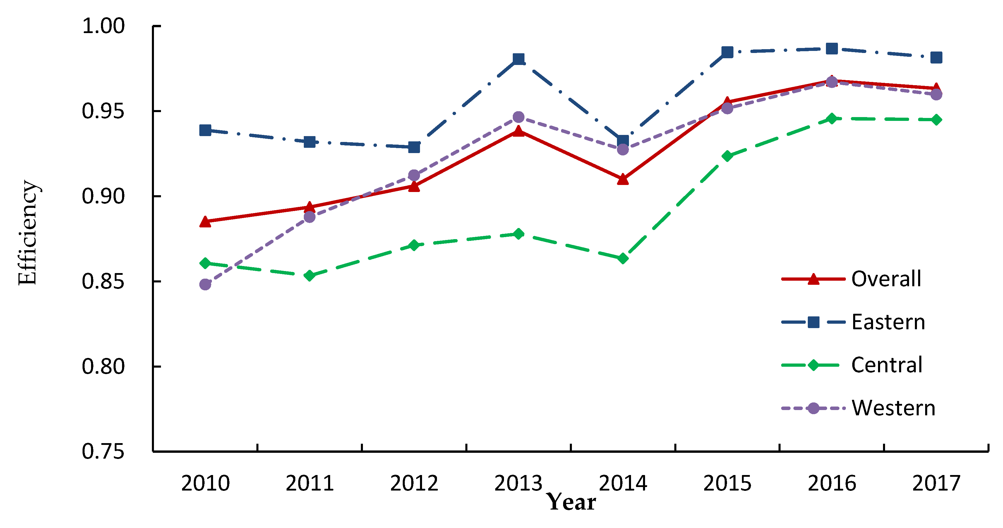
Figure 1 shows the changing trend of environmental efficiency in the whole country, as well as the eastern, central and western areas. The four curves in Figure 1 show an upward trend over time, indicating that the environmental efficiency of road transport is improving from the perspective of development trend, even though the efficiency fluctuates. For the eight years from 2010 to 2017, the eastern area’s environmental efficiency curve is above the overall environmental efficiency curve, while the central area’s environmental efficiency curve is below the overall environmental efficiency curve. For the two years from 2010 to 2011, the curve of the western area is below the overall level. For the three years from 2012 to 2014, the curve of the western area is above the overall level. For 2015 to 2017, the curve of the western area is slightly below the overall level. In 2014, the reduction of environmental efficiency of road transport in eastern areas was large, while that in central and western was small. In 2015, the environmental efficiency of the eastern and central areas increased significantly, while that of the western area increased less than that of the eastern and central areas. The fluctuation range of the environmental efficiency of road transport varies in different regions, and there are obvious regional differences in environmental efficiency of road transport, with the most obvious gap being seen for 2013. With the comprehensive development of the national transport industry, the gap between regions is narrowing. In particular, the environmental efficiency difference between the three areas has been greatly reduced since 2014.

According to

Table 3. Average environmental efficiency of road transport in different areas: 2010–2017.

Area	2010	2011	2012	2013	2014	2015	2016	2017	Mean
Overall	0.8852	0.8936	0.9060	0.9384	0.9101	0.9553	0.9679	0.9633	0.9275
East	0.9388	0.9319	0.9288	0.9805	0.9326	0.9846	0.9867	0.9815	0.9582
Central	0.8607	0.8533	0.8712	0.8779	0.8634	0.9236	0.9457	0.9450	0.8926
West	0.8482	0.8878	0.9123	0.9465	0.9274	0.9516	0.9671	0.9598	0.9251

, differences in the environmental efficiency of road transport can be found in different areas. For 2010 to 2017, the overall average efficiency of road transport is 0.9275. The eastern area with better economic development has the highest average level of environmental efficiency of road transport (0.9582), followed by the western area (0.9251), with the central area having the lowest average efficiency (0.8926). In addition, the western area has the largest efficiency improvement range, with the environmental efficiency score increasing from 0.8482 in 2010 to 0.9598 in 2017; that is, an increase of 0.1166. The environmental efficiency of the central area increased from 0.8607 to 0.9450, an increase of 0.0843. The eastern area figure changed from 0.9388 to 0.9815, increasing by 0.0427.

Regional differences in road transport in China are mainly due to the heterogeneity of economic development level and environment in the areas containing the regions. The eastern area is located in the coastal area, with a developed business system, a strong ability to utilize foreign capital, highly developed infrastructure, great demand for road transport, and many environmental regulations that restrict undesirable output. Therefore, the environmental efficiency value of road transport in the eastern area is relatively high, which is consistent with the empirical results. The central area is an inland region with a large population and a relatively backward level of resources and technology. Furthermore, central China has few environmental regulations and the harmful outputs generated in the process of road transport are not treated promptly, which leads to the lowest environmental efficiency of road transport in these three areas. The western area has a diverse topography, a small population base, and a simple road transport system, so, correspondingly, lower levels of carbon emission, safety accidents, noise pollution, and other adverse outputs compared with the central area. Thus, the environmental efficiency score of road transport in the western area lies between those of the eastern and central areas.

Although there are differences in the average environmental efficiency of the three areas, the differences among them are narrowing. This trend shows that China has achieved some progress in promoting economic development and protecting the ecological environment in the central and western areas, but further improvement remains necessary.

4.2.3. Convergence Analysis at Area Level

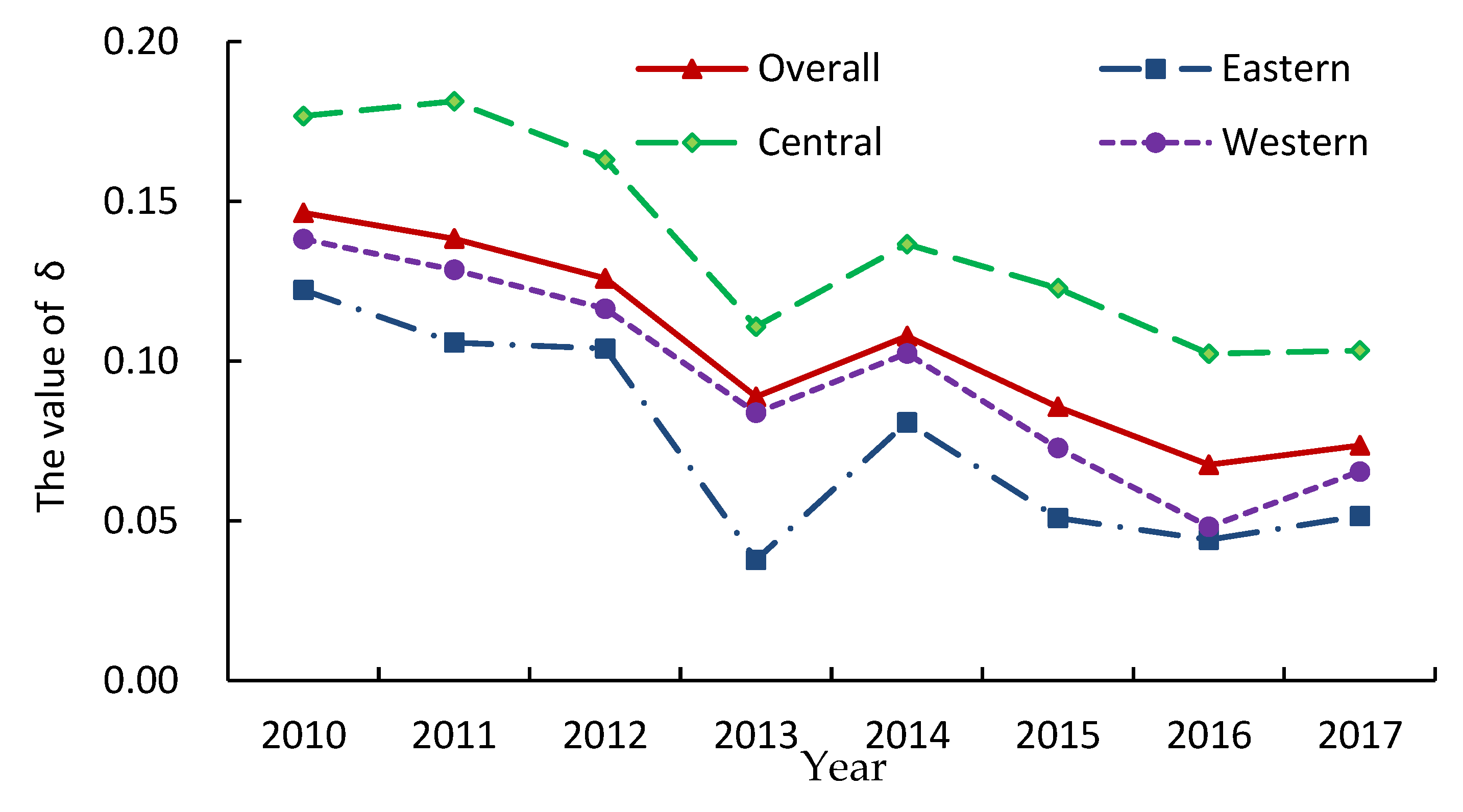
Using Formula (4) above, we conducted σ convergence tests for the whole country and three areas from 2010 to 2017. The results of σ convergence testing are shown in Figure 2. From the point of view of overall environmental efficiency, the standard deviation of environmental efficiency gradually decreased from 2010 to 2013, showing the characteristics of convergence. However, the value of σ rebounded in 2014 and then gradually declined after that, until the value of σ rebounded for a second time in 2017, though the jump was less than that in 2014. Therefore, it can be concluded that during the sample period, the gap in the environmental efficiency between different areas in China is narrowing. That is, there is σ convergence of the national environmental efficiency of road transport. Compared with the overall standard deviation curve, the variation trend of the western area is basically the same as that of the whole country, and the value of σ from 2015 to 2017 is less than that of 2013. Similarly, we can judge that σ convergence exists in the western area.

The trend of change in the eastern and central areas is similar to that in the western area, but the range of change is different. In particular, the standard deviation of the eastern and central areas increased significantly in 2014, and then showed a downward trend, but it was still slightly greater than that of 2013, which is different from the western area. It can be concluded that σ convergence existed in the eastern and central areas at different stages. According to the above analysis, weak σ convergence exists in the eastern and central areas. In addition, the standard deviations of environmental efficiency, from the smallest to the largest, are those of the eastern area, western area, whole country and central area. This phenomenon shows that, compared with the central and western area, the difference in environmental efficiency of road transport between regions within the eastern area is the smallest, and the difference among the central areas is the largest.

Table 4. Absolute β convergence test of environmental efficiency of road transport.

	Overall	Eastern	Central	Western
β	−0.0995 ***	−0.1090 ***	−0.0876 ***	−0.1098 ***
	(0.0094)	(0.0145)	(0.0202)	(0.0174)
α	0.0002	−0.0004	0.0055	−0.0003
F	113.0249	56.5442	18.8743	39.7246
Adjusted R-squared	0.7944	0.8474	0.6908	0.8114

Note: The value in parentheses is the standard error; *, **, ***, indicate significance at 10%, 5%, 1%.

shows that the absolute convergence coefficient of environmental efficiency in the whole country is −0.0995 and passes the significance test at the 1% level, which indicates that the interprovincial environmental efficiency converges to a stable level in China. Moreover, the convergence coefficients of the western, eastern and central areas are −0.1098, −0.1090 and −0.0876, respectively, and all of them pass the significance test at the 1% level, showing that absolute convergence exists in the three areas. That is, the provinces with low environmental efficiency of road transport will gradually catch up with the provinces with high environmental efficiency and finally reach convergence. The western area ranks first in efficiency convergence rate, followed by the eastern area, the whole country and the central area, in that order.

Table 5. Conditional β convergence test of environmental efficiency of road transport.

	Overall	Eastern	Central	Western
β	−0.4849 ***	−0.6403 ***	−0.3466 **	−0.4968 ***
	(0.0584)	(0.0991)	(0.1167)	(0.0844)
α	−0.0296	−0.0250	−0.0317	−0.0258
F	3.0748	4.4179	1.6160	4.5554
Adjusted R-squared	0.2295	0.3310	0.0821	0.3401

Note: The value in parentheses is the standard error; *, **, ***, indicate significance at 10%, 5%, 1%.

shows that the conditional convergence coefficients of the whole country, eastern area and western area are −0.4849, −0.6403 and −0.4968, respectively; these are all significant at the 1% level. In contrast, the convergence coefficient in the central area is −0.3466 and significant only at the 5% level. These results mean that each area has its own steady level and converges to that level.

5. Implications and Conclusions

5.1. Implications

The environmental efficiency of the road transport sector is a topic worthy of study. Many studies only consider carbon dioxide emission or traffic accidents as the only bad output when measuring performance, and there is a lack of relevant research considering multiple undesirable outputs simultaneously. In this paper, the DDF model is employed to measure the environmental efficiency of road transport in mainland China from 2010 to 2017. Compared with previous literature, the main contribution of this paper is to use CO₂ emissions, noise and direct property losses caused by traffic accidents as undesirable outputs when measuring the environmental efficiency of national and regional road transport systems.

The empirical results of this paper reveal the efficiency of the road transport sector more accurately than if only a single undesirable output was considered, so these results play an important role in the formulation of national macro-economic policies. The results show that China’s overall environmental efficiency of road transport is increasing over time, and by 2017, 22 of the 30 regions had the optimal efficiency score. Only five regions maintained optimal efficiency scores in the study period of 2010–2017. However, some regions’ environmental efficiency scores remain inefficient, and historically, some efficient systems have become inefficient (e.g., Beijing in 2014 and 2017). This real and potential inefficiency calls for policymakers to focus on policies to improve and maintain performance. Furthermore, the score of environmental efficiency in developed regions is not necessarily high, and that of underdeveloped regions is not necessarily low, facts which cannot be ignored by local governments. While improving transport efficiency, governments should not ignore the production of undesirable outputs, which certainly affect the environmental efficiency of road transport. Otherwise, these harmful outputs may consume too many human resources, material resources and financial resources, thereby degrading the performance of road transport.

From the broad geographical point of view, there are obvious differences in the road transport industry. The environmental efficiency of road transport is highest in the eastern area, second-highest in the western area and lowest in the central area. Considering the existing gaps, the western area should strengthen its connection with the central and eastern areas and further develop resources to improve environmental efficiency. The central area should attach importance to the negative effect of bad output on environmental efficiency. Overall, all areas should learn from each other’s advantages, try their best to avoid their own disadvantages, and cooperate to promote common development. Furthermore, although there are differences in environmental efficiency among three areas, the differences are constantly narrowing over time, which means that the policies adopted by the central government have played a role in narrowing the gap and should continue to be implemented.

From the overall perspective, the inter-provincial differences in environmental efficiency in China are gradually narrowing with the passage of time. Moreover, absolute β convergence and conditional β convergence exist in the whole country and three areas, reflecting that the growth rate of backward regions is faster than that of developed regions, and each area is converging to its own stable level.

5.2. Conclusions

The purpose of this study was to assess the overall and regional environmental efficiency of road transport from 2010 to 2017, and to analyze the development trend of the regional transport level. Firstly, based on traditional DEA, the DDF model was constructed to include the consideration of a variety of harmful outputs. Secondly, the DDF model and matlab2018 b were used to measure the overall and regional environmental efficiency of road transport in China. Thirdly, a convergence analysis of environmental efficiency was carried out to further test the development trend of overall and regional environmental efficiency.

From 2010 to 2017, the overall environmental efficiency score of road transport increased from 0.8851 to 0.9633, with an overall average score of 0.9275. While the environmental efficiency improved over the study period, the environmental efficiencies of road transport in some provinces are inefficient. Moreover, the environmental efficiency gaps between the eastern, central and western areas have narrowed over time, but still exist. The environmental efficiency of road transport in the eastern area is highest, and is lowest in the central area. The inter-provincial differences in environmental efficiency of road transport are gradually narrowing with the passage of time. The growth rate of environmental efficiency in backward regions is faster than that of developed regions and the environmental efficiency of each area is converging to its own stable level.

Based on the analysis results, suggestions are put forward for decision makers. Firstly, at the national level, the country should attach importance to the technological innovation of road transport and strengthen the environmental regulation to reduce noise and CO₂ emissions. In addition, it is necessary to carry out scientific and effective management of the road transport system to reduce the number of traffic accidents. Secondly, at the geographical area level, the central area should pay more attention to the negative effect of bad output on environmental efficiency and the western area should strengthen its connection with the central and eastern areas. Three areas should learn from each other’s advantages and cooperate to promote common development. Thirdly, at regional (provincial) level, regional governments should attach importance to the innovation and management of road traffic and learn from the advantages of other regions.

Road transport efficiency is also linked to the maintenance cost (i.e., mileage), along with the additional cost caused by the negative externality of the road transport efficiency (e.g., environmental issues, congestion, etc.) In future study, the environmental efficiency of road transport should be studied by considering maintenance and external costs. Furthermore, threshold regression will be carried out to study the relationship between environmental regulation intensity and environmental efficiency of road transport and judge whether there is a threshold effect on the impact of environmental regulation on performance. Accordingly, more theoretical and practical implications can be provided for road transport development.

References

- Chai, J.; Lu, Q.; Wang, S.; Lai, K.K. Analysis of road transportation energy consumption demand in China. Transp. Res. Part D Transp. Environ. 2016, 48, 112–124. [Google Scholar] [CrossRef]
- Xu, X.; Hao, J.; Deng, Y.-R.; Wang, Y. Design optimization of resource combination for collaborative logistics network under uncertainty. Appl. Soft Comput. 2017, 56, 684–691. [Google Scholar] [CrossRef]
- Ministry of Transport of the People’s Republic of China. 2019. Available online: http://xxgk.mot.gov.cn/jigou/zhghs/201904/t20190412_3186720 (accessed on 12 April 2020).
- National Bureau of Statistics of the People’s Republic of China. 2019; China Statistical Yearbook. Available online: http://www.stats.gov.cn/tjsj/zxfb/202002/t20200228_1728913 (accessed on 28 February 2020).
- Wang, D. Assessing road transport sustainability by combining environmental impacts and safety concerns. Transp. Res. Part D Transp. Environ. 2019, 77, 212–223. [Google Scholar] [CrossRef]
- Liu, H.; Zhang, Y.; Zhu, Q.; Chu, J. Environmental efficiency of land transportation in China: A parallel slack-based measure for regional and temporal analysis. J. Clean. Prod. 2017, 142, 867–876. [Google Scholar] [CrossRef]
- World Health Organization. Global status report on road safety. Inj. Prev. 2013, 15, 286. [Google Scholar]
- Mei, G.; Gan, J.; Zhang, N. Metafrontier environmental efficiency for China’s regions: A slack-based efficiency measure. Sustainability 2015, 7, 4004–4021. [Google Scholar] [CrossRef] [Green Version]
- Karlaftis, M.G. A DEA approach for evaluating the efficiency and effectiveness of urban transit systems. Eur. J. Oper. Res. 2004, 152, 354–364. [Google Scholar] [CrossRef]
- Jain, P.; Cullinane, S.; Cullinane, K. The impact of governance development models on urban rail efficiency. Transp. Res. Part A Policy Pract. 2008, 42, 1238–1250. [Google Scholar] [CrossRef]
- Yu, M.-M.; Fan, C.-K. Measuring the performance of multimode bus transit: A mixed structure network DEA model. Transp. Res. Part E Logist. Transp. Rev. 2009, 45, 501–515. [Google Scholar] [CrossRef]
- Kumar, S. State road transport undertakings in India: Technical efficiency and its determinants. Benchmarking Int. J. 2011, 18, 616–643. [Google Scholar] [CrossRef]
- Yang, T.; Guan, X.; Qian, Y.; Xing, W.; Wu, H. Efficiency evaluation of urban road transport and land use in Hunan Province of China based on hybrid Data Envelopment Analysis (DEA) models. Sustainability 2019, 11, 3826. [Google Scholar] [CrossRef] [Green Version]
- Holmgren, J. The efficiency of public transport operations—An evaluation using stochastic frontier analysis. Res. Transp. Econ. 2013, 39, 50–57. [Google Scholar] [CrossRef] [Green Version]
- Jarboui, S.; Forget, P.; Boujelbène, Y.; Boujelben, Y. Efficiency evaluation in public road transport: A stochastic frontier analysis. Transport 2013, 30, 1–14. [Google Scholar] [CrossRef] [Green Version]
- Ayadi, A.; Hammami, S. An analysis of the performance of public bus transport in Tunisian cities. Transp. Res. Part A Policy Pract. 2015, 75, 51–60. [Google Scholar] [CrossRef]
- Wang, Z.; He, W. CO2 emissions efficiency and marginal abatement costs of the regional transportation sectors in China. Transp. Res. Part D Transp. Environ. 2017, 50, 83–97. [Google Scholar] [CrossRef]
- Ma, F.; Li, X.; Sun, Q.; Liu, F.; Wang, W.; Huang, K. Regional differences and spatial aggregation of sustainable transport efficiency: A case study of China. Sustainability 2018, 10, 2399. [Google Scholar] [CrossRef] [Green Version]
- Bian, J.; Zhao, X. Tax or subsidy? An analysis of environmental policies in supply chains with retail competition. Eur. J. Oper. Res. 2020, 283, 901–914. [Google Scholar] [CrossRef]
- Tang, T.; You, J.; Sun, H.; Zhang, H. Transportation efficiency evaluation considering the environmental impact for China’s freight sector: A parallel data envelopment analysis. Sustainability 2019, 11, 5108. [Google Scholar] [CrossRef] [Green Version]
- Färe, R.; Grosskopf, S. Directional distance functions and slacks-based measures of efficiency. Eur. J. Oper. Res. 2010, 200, 320–322. [Google Scholar] [CrossRef]
- Wang, K.; Wei, Y.-M.; Zhang, X. Energy and emissions efficiency patterns of Chinese regions: A multi-directional efficiency analysis. Appl. Energy 2013, 104, 105–116. [Google Scholar] [CrossRef]
- Xie, B.-C.; Shang, L.-F.; Yang, S.-B.; Yi, B.-W. Dynamic environmental efficiency evaluation of electric power industries: Evidence from OECD (Organization for Economic Cooperation and Development) and BRIC (Brazil, Russia, India and China) countries. Energy 2014, 74, 147–157. [Google Scholar] [CrossRef]
- Zhou, G.; Chung, W.; Zhang, Y. Measuring energy efficiency performance of China’s transport sector: A data envelopment analysis approach. Expert Syst. Appl. 2014, 41, 709–722. [Google Scholar] [CrossRef]
- Agarwal, S.; Yadav, S.P.; Singh, S. DEA based estimation of the technical efficiency of state transport undertakings in India. Opsearch 2010, 47, 216–230. [Google Scholar] [CrossRef]
- Liu, Z.; Qin, C.-X.; Zhang, Y.-J. The energy-environment efficiency of road and railway sectors in China: Evidence from the provincial level. Ecol. Indic. 2016, 69, 559–570. [Google Scholar] [CrossRef]
- Pal, D.; Mitra, S.K. An application of the directional distance function with the number of accidents as an undesirable output to measure the technical efficiency of state road transport in India. Transp. Res. Part A Policy Pract. 2016, 93, 1–12. [Google Scholar] [CrossRef]
- Park, Y.S.; Lim, S.H.; Egilmez, G.; Szmerekovsky, J. Environmental efficiency assessment of U.S. transport sector: A slack-based data envelopment analysis approach. Transp. Res. Part D Transp. Environ. 2018, 61, 152–164. [Google Scholar] [CrossRef] [Green Version]
- Wu, J.; Zhu, Q.; Chu, J.; Liu, H.; Liang, L. Measuring energy and environmental efficiency of transportation systems in China based on a parallel DEA approach. Transp. Res. Part D Transp. Environ. 2016, 48, 460–472. [Google Scholar] [CrossRef]
- Piccioni, D.I.C. Territorial accessibility and dynamics in road infrastructures use: An integrated planning approach. Ing. Ferrov. 2011, 66, 621–641. [Google Scholar]
- Wang, T.; Li, H.; Zhang, J.; Lu, Y. Influencing factors of carbon emission in China’s road freight transport. Proc. Soc. Behav. 2012, 43, 54–64. [Google Scholar] [CrossRef] [Green Version]
- Omrani, H.; Shafaat, K.; Alizadeh, A. Integrated data envelopment analysis and cooperative game for evaluating energy efficiency of transportation sector: A case of Iran. Ann. Oper. Res. 2018, 274, 471–499. [Google Scholar] [CrossRef]
- Yang, H.; Pollitt, M.G. Incorporating both undesirable outputs and uncontrollable variables into DEA: The performance of Chinese coal-fired power plants. Eur. J. Oper. Res. 2009, 197, 1095–1105. [Google Scholar] [CrossRef] [Green Version]
- Fan, L.; Wu, F.; Zhou, P. Efficiency measurement of Chinese airports with flight delays by directional distance function. J. Air Transp. Manag. 2014, 34, 140–145. [Google Scholar] [CrossRef]
- Chung, Y.; Färe, R.; Grosskopf, S. Productivity and undesirable outputs: A directional distance function approach. J. Environ. Manag. 1997, 51, 229–240. [Google Scholar] [CrossRef] [Green Version]
- Färe, R.; Grosskopf, S.; Pasurka, C. Environmental production functions and environmental directional distance functions. Energy 2007, 32, 1055–1066. [Google Scholar] [CrossRef]
- Martini, G.; Manello, A.; Scotti, D. The influence of fleet mix, ownership and LCCs on airports’ technical/environmental efficiency. Transp. Res. Part E Logist. Transp. Rev. 2013, 50, 37–52. [Google Scholar] [CrossRef]
- Chambers, R.G.; Chung, Y.; Färe, R. Profit, directional distance functions, and nerlovian efficiency. J. Optim. Theory Appl. 1998, 98, 351–364. [Google Scholar] [CrossRef]
- Charnes, A.; Cooper, W.; Rhodes, E. Measuring the efficiency of decision making units. Eur. J. Oper. Res. 1978, 2, 429–444. [Google Scholar] [CrossRef]
- Solarin, S.A. Convergence in CO 2 emissions, carbon footprint and ecological footprint: Evidence from OECD countries. Environ. Sci. Pollut. Res. 2019, 26, 6167–6181. [Google Scholar] [CrossRef]
- Erdogan, S.; Acaravci, A. Revisiting the convergence of carbon emission phenomenon in OECD countries: New evidence from Fourier panel KPSS test. Environ. Sci. Pollut. Res. 2019, 26, 24758–24771. [Google Scholar] [CrossRef]
- Barro, R.J.; Sala-I-Martin, X.; Hall, O.J.B.E. Convergence across states and regions. Brook. Pap. Econ. Act. 1991, 1991, 107. [Google Scholar] [CrossRef] [Green Version]
- Bhattacharya, M.; Inekwe, J.; Sadorsky, P. Convergence of energy productivity in Australian states and territories: Determinants and forecasts. Energy Econ. 2020, 85, 104538. [Google Scholar] [CrossRef]
- Miller, S.M.; Upadhyay, M.P. Total factor productivity and the convergence hypothesis. J. Macroecon. 2002, 24, 267–286. [Google Scholar] [CrossRef]
- Liu, H.; Wu, J.; Chu, J. Environmental efficiency and technological progress of transportation industry-based on large scale data. Technol. Forecast. Soc. Chang. 2019, 144, 475–482. [Google Scholar] [CrossRef]
- Gao, Y.; Li, W.D.; You, X.Y. Research on the efficiency evaluation of China’s railway transport enterprises with Network DEA. China Soft Sci. 2011, 5, 176–182. [Google Scholar]
- Song, M.; Zheng, W.; Wang, Z. Environmental efficiency and energy consumption of highway transportation systems in China. Int. J. Prod. Econ. 2016, 181, 441–449. [Google Scholar] [CrossRef]
- Cui, Q.; Li, Y. An empirical study on the influencing factors of transportation carbon efficiency: Evidences from fifteen countries. Appl. Energy 2015, 141, 209–217. [Google Scholar] [CrossRef]
- Chen, X.; Gao, Y.; An, Q.; Wang, Z.; Neralić, L. Energy efficiency measurement of Chinese Yangtze River Delta’s cities transportation: A DEA window analysis approach. Energy Effic. 2018, 11, 1941–1953. [Google Scholar] [CrossRef]
- Egbetokun, S.; Osabuohien, E.; Akinbobola, T.; Onanuga, O.T.; Gershon, O.; Okafor, V. Environmental pollution, economic growth and institutional quality: Exploring the nexus in Nigeria. Manag. Environ. Qual. Int. J. 2020, 31, 18–31. [Google Scholar] [CrossRef] [Green Version]
Figure 1.
Variation trend of environmental efficiency in different areas.
Figure 2.
σ convergence test of environmental efficiency of road transport.