Density Estimation of Antarctic Krill in the South Shetland Island (Subarea 48.1) Using dB-Difference Method

Abstract

This study is aimed to estimate the density of Antarctic krill that inhabit in the area around South Shetland Island by using a dB-difference method. An acoustic survey was conducted from 13 to 24 April in 2016 in the sea of South Shetland. Acoustic data on frequency 38 and 120 kHz were collected. The Antarctic krill echo was extracted for the S_{V120-38 kHz} range of 0.4–14.3 dB, which was obtained by applying the size of the collected Antarctic krill in this study (25–60 mm). The mean Antarctic krill density across the survey area was 33.65 g m⁻² (CV = 45.97%).

1. Introduction

Antarctic krill (Euphausia superba) play an important role as part of the Antarctic marine ecosystem, with recent research focusing on their potential as a future alternative food source for use in the development of various health foods and medications [1,2,3,4,5]. However, global warming, changes in the marine environment, and the overfishing of Antarctic krill resources have caused their decline, impacting the marine ecosystem itself. In an effort to resolve these issues, the Commission for the Conservation of Antarctic Marine Living Resources (CCAMLR) was formed in 1982 for the sustainable conservation and logical use of marine organisms inhabiting Antarctic waters. At present, the CCAMLR has 25 member states. South Korea joined the CCAMLR in 1985, and, in collaboration with the other member states, has been conducting surveys and research, participating in international surveillance operations of the Antarctic marine ecosystem and marine organisms [6,7].

In particular, Antarctic krill are a major food source for marine animals, such as penguins, seals, and whales. Because of this, the CCAMLR has implemented systematic control measures for Antarctic krill resources since 1982, such as restricting total catch volumes. In addition, there have been collaborative research efforts to improve the management of Antarctic krill resources, with a strong focus on the countries that catch Antarctic krill. In order to manage Antarctic krill resources, research must be conducted to understand the distribution and abundance of Antarctic krill. Acoustic technology is often used to evaluate the spatiotemporal distribution and abundance of Antarctic krill, because it provides information at all depths, over a wide area, and in a short time [5,8,9,10]. The CCAMLR-2000 Antarctic krill Synoptic Survey was designed, planned, and implemented in 1995 to conduct acoustic surveys of Antarctic krill resources [11]. The Subgroup on Acoustic Survey and Analysis Method (SG-ASAM) has been in action since 2011.

Antarctic krill fishing operations take place in waters around the South Shetland Islands (Subarea 48.1), the South Orkney Islands (Subarea 48.2), South Georgia (Subarea 48.3), and South Sandwich (Subarea 48.4). The total catch sizes are restricted to 155,000 tons in the South Shetland Islands (Subarea 48.1), 279,000 tons in the South Orkney Islands (Subarea 48.2), 279,000 tons in South Georgia (Subarea 48.3), and 93,000 tons in South Sandwich (Subarea 48.4). Information on the abundance of Antarctic krill is required to set an upper limit to the total allowed catch volume. The abundance of Antarctic krill populations in these waters is continually assessed and reported based on acoustic surveys. In the present study, we used acoustic data collected through CCAMLR analytical methods to determine the distribution and density of Antarctic krill inhabiting the waters near the South Shetland Islands (Subarea 48.1).

2. Materials and Methods

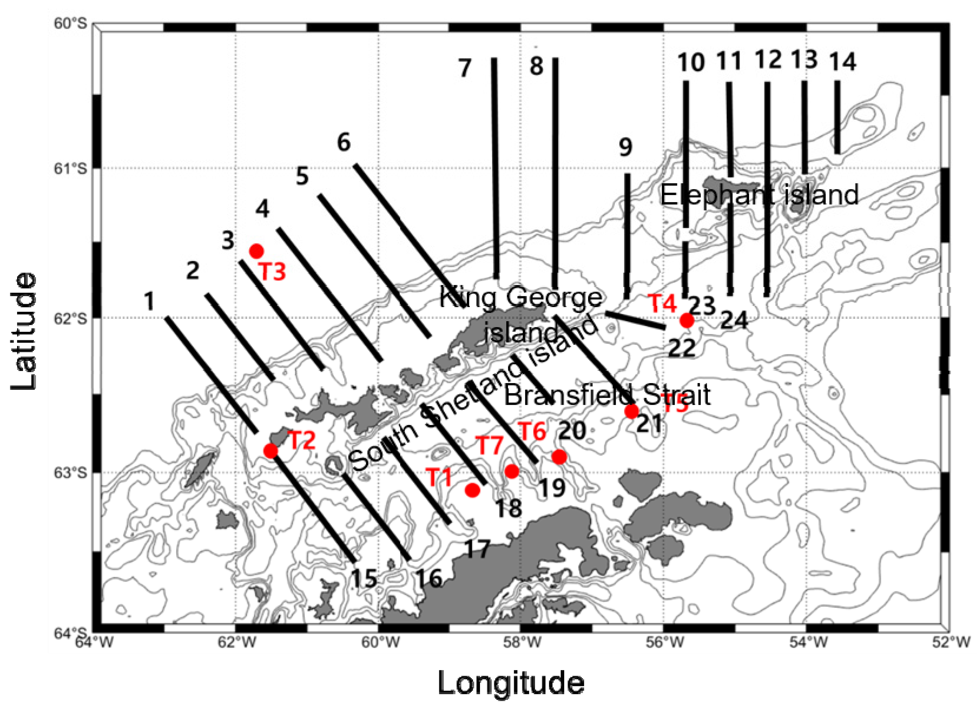
2.1. Survey Area and Sampling Sites

The survey area covered the west of South Shetland Islands, Elephant Island, and Bransfield Strait in the south. The survey area consisted of the coastal area, formed by the continental shelf within 200 m of the islands, the tidal front at the interface of different types of water, and the offshore area where the water became deeper.

The survey was conducted using a commercial fishing vessel (Gwangja-ho), from 13 to 24 April 2016. The survey area was 90,700 km², within which 24 survey lines and seven sampling locations were established (Figure 1). Acoustic data were recorded while travelling along the survey lines at a speed of <10 knots, and organisms were collected at the sampling points using a midwater trawl. The towing speed of the trawl was maintained at 2–3 knots.

2.2. Acoustic System Setup and Data Collection

For the acoustic survey system, we used a split-beam scientific echosounder (EK60, Simrad, Norway) attached to the bottom of the Gwangja-ho at frequencies of 38 and 120 kHz. The parameters of the system during acoustic surveys were set according to the criteria presented by the CCAMLR (

Table 1. Scientific echosounder set up to collect acoustic data.

Parameters	Setting
Frequency (kHz)	38	120
Power setting (w)	2000	250
Ping duration (ms)	1.024	1.024
Ping interval (s)	2	2
Data collection range (min.-max.) (m)	0–1100	0–1100
Bottom detection range (min.-max.) (m)	5–1100	5–1100
Display range (min.-max.) (m)	0–1100	0–1100

). Before the survey, the echosounder was calibrated at the coast using 60 mm at 38 kHz and 23 mm at 120 kHz copper spheres following the method of Foote et al. [12] (62°28.7′ S, 59°42.4′ W). The results of calibration are shown in Table 1 and

Table 2. Results of calibration at frequencies of 38 and 120 kHz.

Frequency (kHz)	38	120
Two-way beam angle (dB)	−20.6	−21.0
Receiver bandwidth (kHz)	2.43	3.03
Transducer gain (dB)	26.82	27.64
3-dB Beam angle (athwart/along) (deg.)	7.08/7.03	6.47/5.60
Absorption coefficient (dB km−1)	9.8	24.7
Sound speed (m s−1)	1448.9	1448.9

.

2.3. Antarctic Krill Sampling

The Antarctic krill were collected with a midwater trawl used on a commercial fishing ship. The total net length was 167.6 m, the mesh size was 15 mm, the net height was 40 m, and the net width was 72 m. The biomass of each sample was measured after hauling. At each sampling point, 200 Antarctic krill were randomly selected, and the length was measured at 1 mm intervals from the anterior margin of the eye to the tip of the telson, excluding the terminal spines.

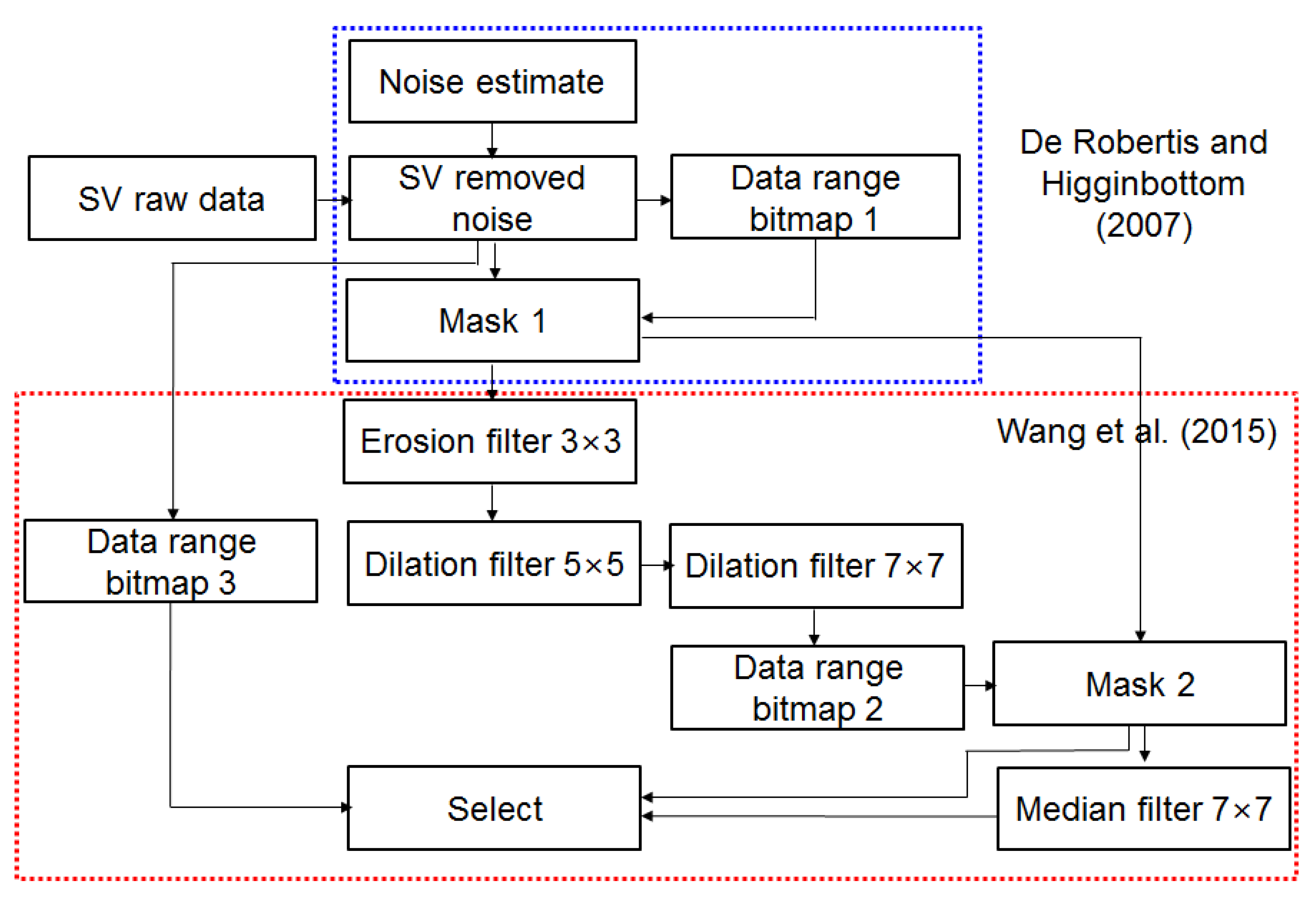
2.4. Analysis of Acoustic Data

The collected acoustic data were analyzed using acoustic analysis software (Echoview V 8.0, Echoview Software, Australia). Noise from the ship and from electric signals was removed using the methods of De Robertis and Higginbottom and Wang et al. [13,14]. Figure 2 and Figure 3 present a flowchart used for noise reduction and an example echogram following processing. The survey area in this study had a depth of over 1000 m, and background noise increased at greater depths. The time varied threshold (TVT) method was used to remove this noise. This approach involves artificially creating background noise, and then removing it from the raw data. Any remaining noise was removed by using a data range bitmap to eliminate noise smaller than the minimum volume backscattering strength (S_V) of Antarctic krill and larger than the maximum S_V of Antarctic krill, and then masking it [13]. In the data range bitmap, Antarctic krill were used as the true value, and all other values were used as false values. Although the implemented method was sufficient to remove most of the noise, an erosion filter 3 × 3 function was also used to remove any remaining noise. The 3 × 3 function is the cell range, wherein the filter converts each cell to the minimum value of the surrounding cells within this range; since the surrounding noise of the cells was −999 dB, this caused all noise to disappear. Although this process removes all the noise, the echo signal is weakened, and empty spaces within the original data lead to the loss of the echo shape. A dilation filter function was used to restore lost signal, by converting each cell to the maximum of its surrounding cells to fill in empty spaces in the echo. Cell ranges of 5 × 5 and 7 × 7 were used in sequence to fill in the empty spaces in the echogram. After applying the dilation filter 7 × 7 function, a data range bitmap function was used to generate a mask for the echogram, which was set to the S_V range of Antarctic krill. Finally, a median 7 × 7 function was applied, which converts each cell to the median of its surrounding cells, before generating a data range bitmap from the noise-corrected S_V echogram and the echo previously selected using the mask and median 7 × 7 function, and using a select operator to obtain the Antarctic krill signal with the noise clean removed [14].

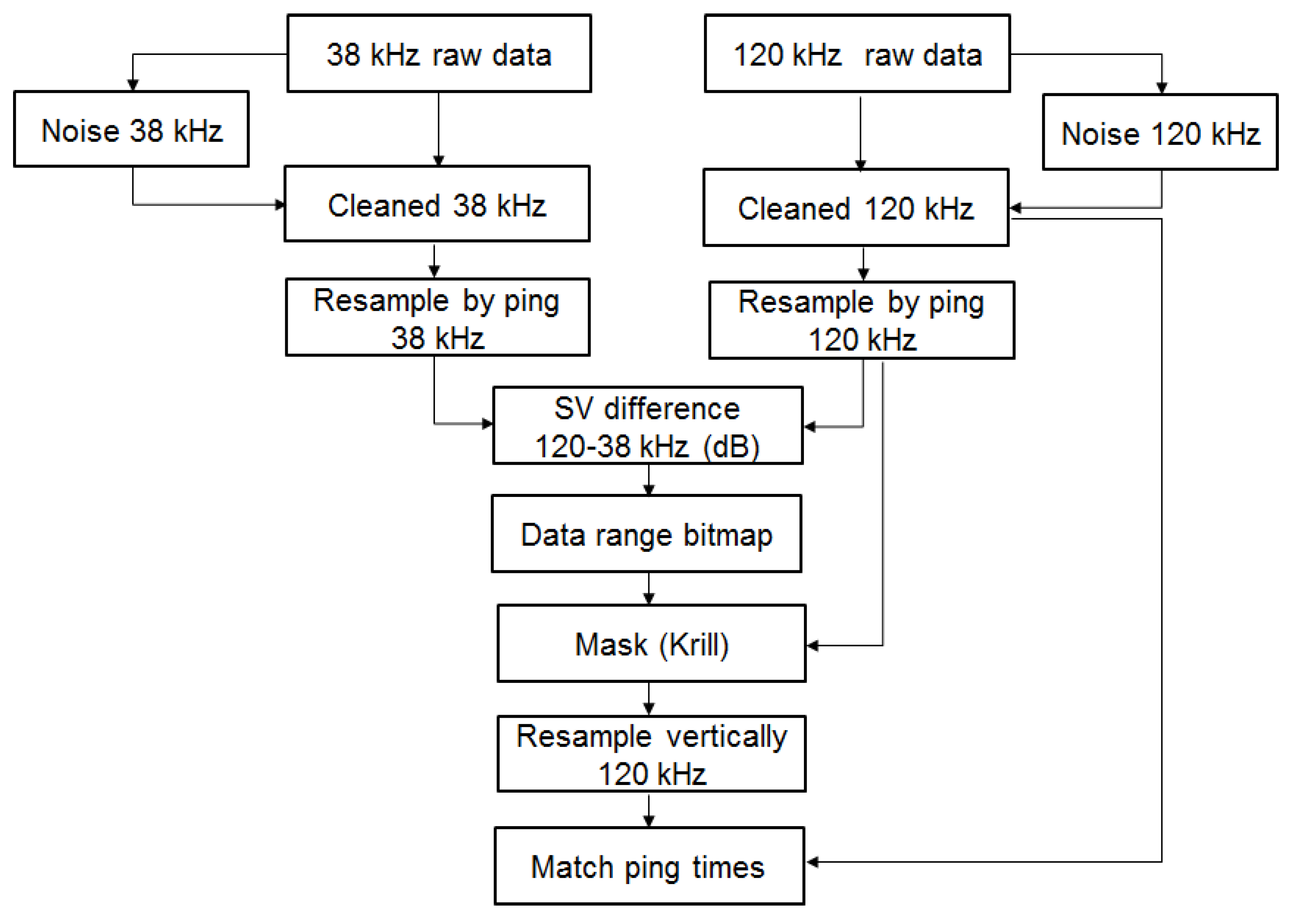
2.5. dB Differences and Extraction of Antarctic Krill Echoes

To extract the Antarctic krill echoes, the characteristics of the frequency and differences between 38 and 120 kHz in Antarctic krill must be understood. Frequency characteristics and differences are used to clearly differentiate species. The dB differences of multi-frequency data are differences in the mean volume backscattering strength (MVBS). To ensure a positive value, ΔMVBS was calculated by comparing target strength (TS) for the target species at the different frequencies, and by subtracting the smaller TS from the larger TS. Typically, zooplankton show a stronger signal at 120 kHz than at 38 kHz. Therefore, ΔMVBS may be obtained from a new echogram formed of a matrix combining the 38 and 120 kHz signals, using the following Equation (1).

$$\mathsf{\Delta }\mathrm{MVBS}=\mathrm{TS}\left(120 \mathrm{kHz}\right)-\mathrm{TS}\left(38 \mathrm{kHz}\right)=S_V\left(120 \mathrm{kHz}\right)-S_V\left(38 \mathrm{kHz}\right)$$

(1)

Figure 4 presents a flow chart on how data were processed to examine dB differences of Antarctic krill and to identify species. After filtering out the sea surface noise, sea bottom noise, and other noise, if an interval of integration is selected, a new echogram was generated as a matrix combining the two frequencies. The cell dimensions (width × height) used to inspect inter-frequency differences in this study were 50 ping × 5 m.

Once the difference in the inter-frequency for Antarctic krill was established, the range of differences was used to make a data range bitmap, which was then used to make a mask matching the cell size at 120 kHz. Then, after dividing the cells into pings, the mask was applied to the noise-corrected 120 kHz echo to provide the Antarctic krill echo. This method allows Antarctic krill to be identified by extracting the Antarctic krill echo that fits these characteristics, rather than the frequency characteristics of Antarctic krill.

The range of dB differences used to identify Antarctic krill was the recommended range of S_V differences (min-max) based on the size distribution of Antarctic krill by CCAMLR 2010 [11]. Antarctic krill body length was determined using the maximum and minimum size of Antarctic krill collected from the study area.

2.6. Density Calculation

Antarctic krill density was calculated, using the dB difference, as the acoustic scatter at 120 kHz integrated over 1 n.mile horizontally and vertically from the surface to 5 m above the sea bottom. The extracted data were the scatter area in the presence of Antarctic krill integrated over the n.mile of each survey line ($s_A$, m² nmi⁻²), where $s_A$ is expressed as the nautical area scattering coefficient (NASC), which is calculated as the linear sum of the signal received from organisms within a given volume. The scatter area is converted by applying the density of Antarctic krill per 1 n.mile within the target volume to the conversion factor C. C is calculated, before combining it with the conversion factor, using the weighted mean backscattering cross sectional area ($\mathsf{\sigma }$, m²) and the weight (w, g).

$$\mathsf{\rho }=s_{A}C\times {1852}^2\left(\frac{g}{m^2}\right)$$

(2)

where

$$C=\frac{{\displaystyle \sum }{f}_i\times w\left(l_i\right)}{{\displaystyle \sum }{f}_i\times \sigma \left(l_i\right)}$$

(3)

where $f_i$ is the i^th bin along the length $l_i$.

The length-weight relationship of Antarctic krill was calculated using data measured from the research vessel Kaiyo Maru in CCMALR 2000.

$$\mathrm{w}=2.236\times {10}^{-6}{l}^{3.314}$$

(4)

where the weight is total weight (mg) and body length is total length (mm).

For the backscattering cross-sectional area of Antarctic krill, we applied the TS that stochastic distorted wave Born approximation (SDWBA) was selected as the TS model by CCAMLR 2010 [11].

$${\mathsf{\sigma }}_{sp}=4\mathsf{\pi }{10}^{TS/10}$$

(5)

The mean Antarctic krill density was calculated for all intervals (index i) of all survey lines (index j) within all survey areas (index k).

$$\overline{{\rho }_j}=\frac{1}{L_j}{\displaystyle \sum }_{i=1}^{N_j}\frac{s_{Ai}{C}_i{W}_1{}_i}{{1852}^2}$$

(6)

where $L_j={{\displaystyle \sum }}_{i=1}^{N_i}{(W_1)}_i$ is the length of the j^th transverse section, defined as the weighted sum of all intervals. $s_{Ai}$ is the integrated area scattering coefficient for the i^th interval, and $C_j$ is the i^th conversion factor.

Deviation from the survey lines due to strong winds, currents, or icebergs was corrected by comparing the predicted change in latitude ($\mathsf{\Delta }\mathrm{lat}$) per 1 nautical mile with the actual latitude interval to produce a favorable course ($\mathsf{\Delta }\mathrm{l}\widehat{a}t$) using the weighted interval, $W_1$.

$$W_1=\frac{\left|\mathsf{\Delta }lat\right|-\left|\mathsf{\Delta }lat-\mathsf{\Delta }l\widehat{a}t\right|}{\left|\mathsf{\Delta }lat\right|}$$

(7)

If the deviation from the standard line for a specific interval was 10% or greater (i.e., if $W_1<0.9$), the integral weighted value of 1 nm was expanded to make $W_1=1$.

The weight of Antarctic krill density was calculated as the product of the mean area Antarctic krill density and the weight coefficient derived from the normalized length of the survey line.

$$w_j=\frac{L_j}{\frac{1}{N}{{\displaystyle \sum }}_{j=1}^{N_k}{L}_j}$$

(8)

where $N_k$ is the number of survey lines with the survey area. The mean weighted area for Antarctic krill density in the j^th survey line ($\overline{{\rho }_{wJ}}$) was calculated by Equation (9).

$$\overline{{\rho }_k}=\frac{1}{N}{\displaystyle \sum }_{j=1}^{N_k}{w}_j\overline{{\rho }_j}$$

(9)

The variance component ($VarCom{p}_j$) is the j^th weight in the deviation within the survey area.

$$Varcom{p}_j=w_j^2{(\overline{{\rho }_J}-\overline{{\rho }_k})}^2$$

(10)

The mean area Antarctic krill density in the k^th survey area (after Equation (2), [16]) can be expressed as in Equation (11).

$$\overline{{\rho }_k}=\frac{1}{N}{\displaystyle \sum }_{j=1}^{N_k}{w}_j\overline{{\rho }_j}$$

(11)

Here, the variance of the mean Antarctic krill density in the k^th survey area ($\mathrm{Var}\left(\overline{{\rho }_k}\right)$ is:

$$\mathrm{Var}\left(\overline{{\rho }_k}\right)=\frac{{{\displaystyle \sum }}_{j=1}^{N_k}{w}_j^2{}_{{(\overline{{\rho }_j}-\overline{{\rho }_k})}^2}}{N_k\left(N_k-1\right)}$$

(12)

The coefficient of variation (%) for the k^th survey area ($C{V}_k$) is given by:

$$C{V}_k=100\frac{\sqrt{(Var\left(\overline{{\rho }_k}\right)}}{\overline{{\rho }_k}}$$

(13)

3. Results

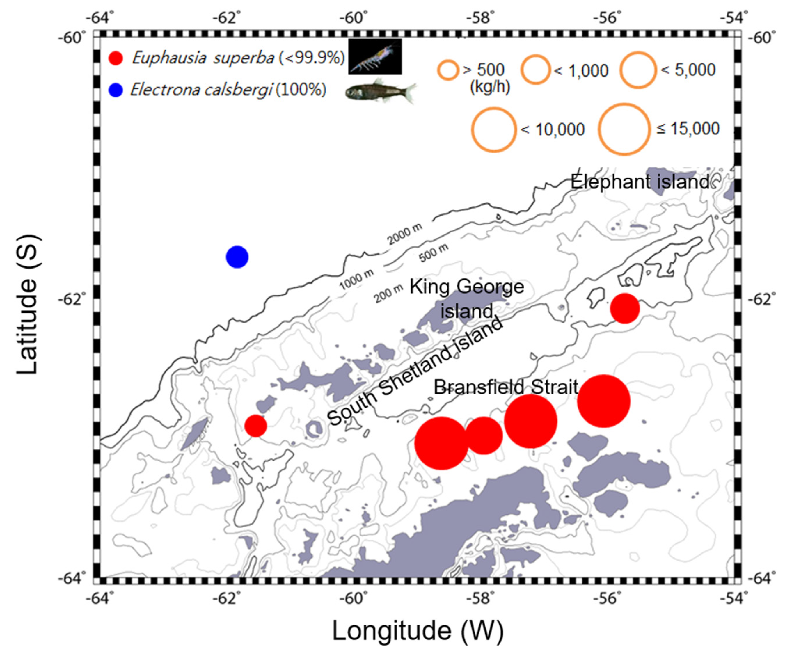
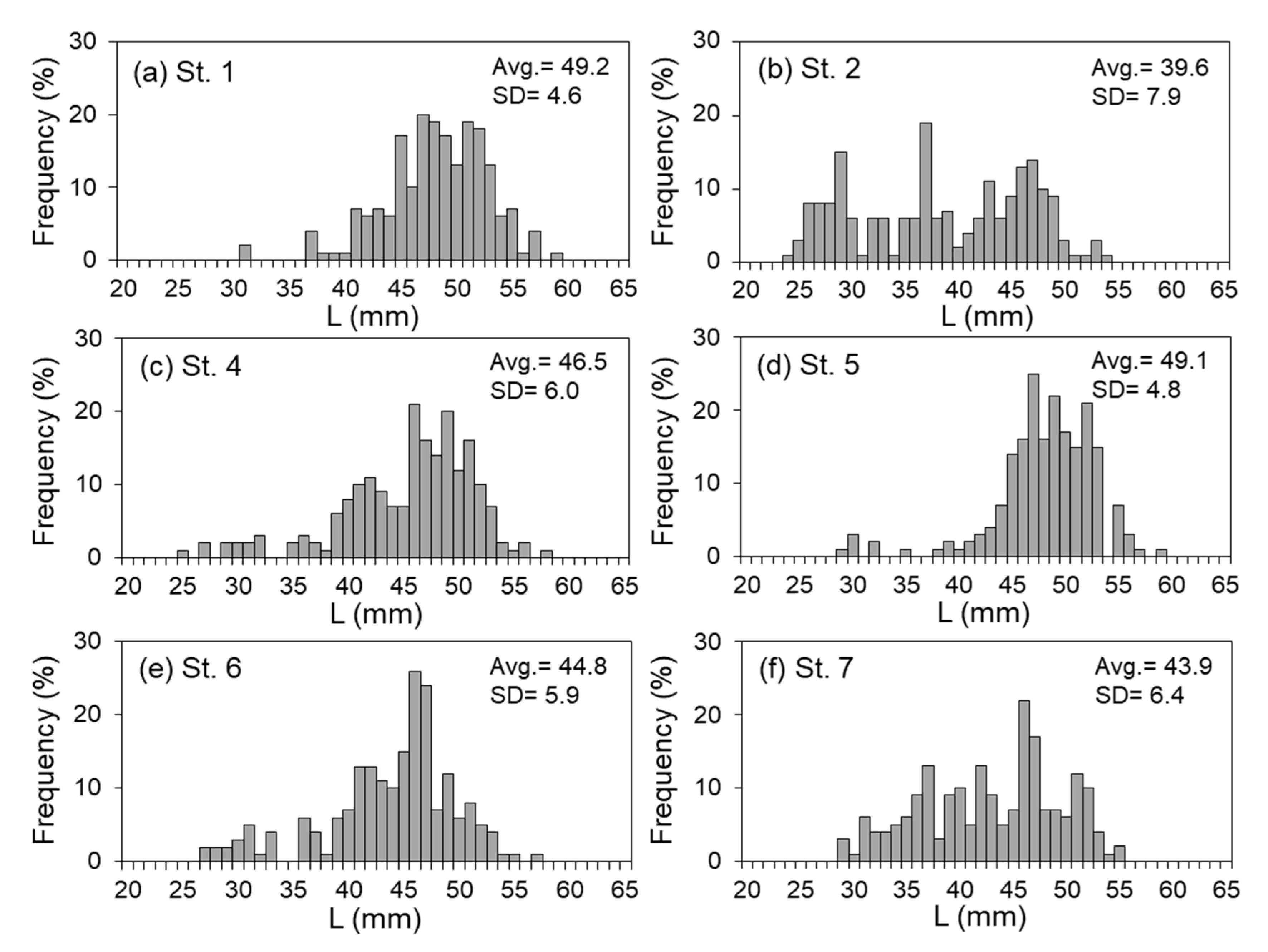
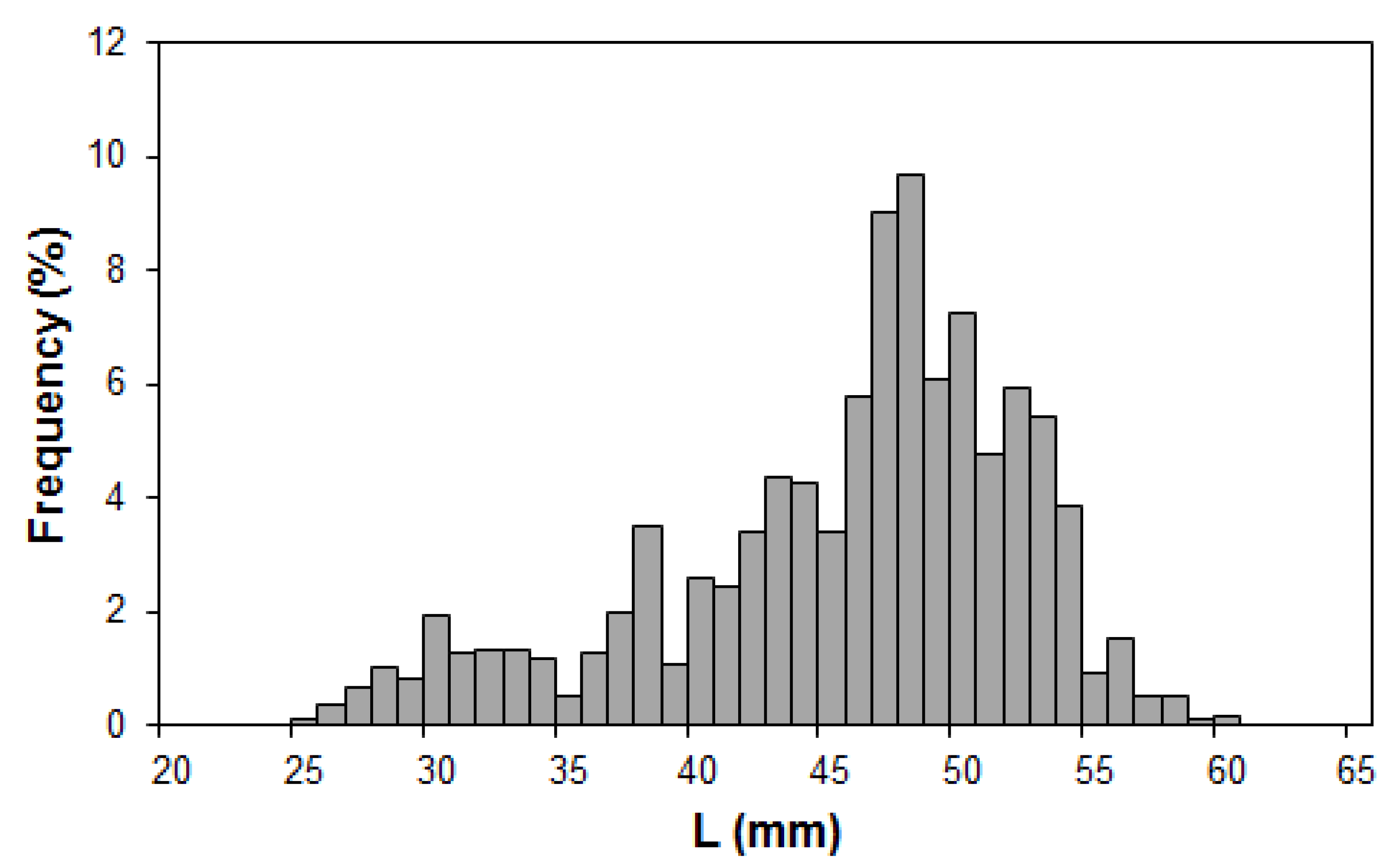
3.1. Collected Samples and Size Distribution

Table 3. Trawling time, sampling point, location, towing time, depth, contents of catch, and catch size (KRI: Antarctic krill, Euphausia superba; WIC: Spiny icefish, Chaenodraco wilsoni; FIC: Long-fingered icefish, Crydraco antarcticus; KIF: Ocellated icefish, Chaenodraco rastrospinosus; ELC: Lanternfish, Electrona carlsbergi; PSG: Glacial squid, Psychroteuthis glacialis).

Station	Date (DD Month YYYY)	Latitude (S)	Longitude (W)	Towing Time (Minute)	Towing Depth (m)	Bottom Depth (m)	Catch (kg)	Antarctic Krill Ratio (%)
1	14 April 2016	63°3.1′	58°35.8′	53	50–80	180	KRI: 10,149WIC: 0.52FIC: 0.03	99.9
2	16 April 2016	62°55.2′	61°35.7′	60	30–60	178	KRI: 357WIC: 0.42PSG: 0.01	99.9
3	17 April 2016	61°40.4′	61°53.9′	32	180–210	<3000	ELC: 0.1	0.0
4	20 April 2016	61°1.5′	55°45.4′	14	90–120	140	KRI: 179FIC: 0.1ELC: 0.54	99.9
5	22 April 2016	62°37.7′	56°18.1′	24	240–270	300	KRI: 7925KIF: 0.64	99.9
6	23 April 2016	62°56.2′	57°20.6′	43	90–120	143	KRI: 10,308WIC: 0.44FIC: 0.01	99.9
7	23 April 2016	62°59.2′	57°55.6′	37	110–140	490	KRI: 2514WIC: 0.03FIC: 0.04	99.9

shows the results of the trawl surveys from seven sampling points in the survey area. In total, 10,149 kg Antarctic krill, 0.52 kg spiny icefish (Chaenodraco wilsoni), and 0.03 kg long-fingered icefish (Cryodraco antarcticus) were caught at Station (St.) 1; 357 kg Antarctic krill, 0.42 kg spiny icefish, and 0.01 kg glacial squid (Psychroteuthis glacialis) were caught at St. 2; 0.1 kg lanternfish (Electrona carlsbergi) were caught at St. 3; 179 kg Antarctic krill, 0.1 kg long-fingered icefish, and 0.54 kg lanternfish were caught at St. 4; 7925 kg Antarctic krill and 0.64 kg ocellated icefish (Chionodraco rastrospinosus) were caught at St. 5; 10,308 kg Antarctic krill, 0.44 kg spiny icefish, and 0.01 kg ocellated icefish were caught at St. 6; and 2514 kg Antarctic krill, 0.03 kg spiny icefish, and 0.04 kg ocellated icefish were caught at St. 7. Thus, excluding St. 3, at which only lanternfish were caught, over 99.9% of the catch at the other six sampling points was Antarctic krill.

The catch per unit effort (CPUE, kg/h) for Antarctic krill was 11,489.4 kg/h at St. 1, 357.0 kg/h at St. 2, 767.1 kg/h at St. 4, 19,812.5 kg/h at St. 5, and 4076.8 kg/h at St. 6. The CPUE for lanternfish was 0.2 kg/h at St. 3. Mostly Antarctic krill were caught up to a depth of 500 m, while lanternfish were caught at depths of over 3000 m. Antarctic krill were caught in particularly large numbers to the south of the South Shetland Islands (Figure 5).

The size (L, mm) of the caught Antarctic krill at each sampling point was: 32.0–60.0 mm (Avg. ± SD = 49.2 ± 4.6 mm) at St. 1, 25.0–55.0 mm (39.6 ± 7.9 mm) at St. 2, 26.0–59.0 mm (46.5 ± 6.0 mm) at St. 4, 30.0–60.0 mm (49.1 ± 4.8 mm) at St. 5, 28.0–58.0 mm (44.8 ± 5.9 mm) at St. 6, and 30.0–56.0 mm (43.9 ± 6.4 mm) at St. 7. Hence, more small individuals were caught at St. 2 compared to the other sampling points (Figure 6). A cross all sampling points, the Antarctic krill were 25.0–60.0 mm (Avg. ± SD = 45.5 ± 6.9 mm) in size, and the distribution was unimodal with the mode at 48 mm (Figure 7).

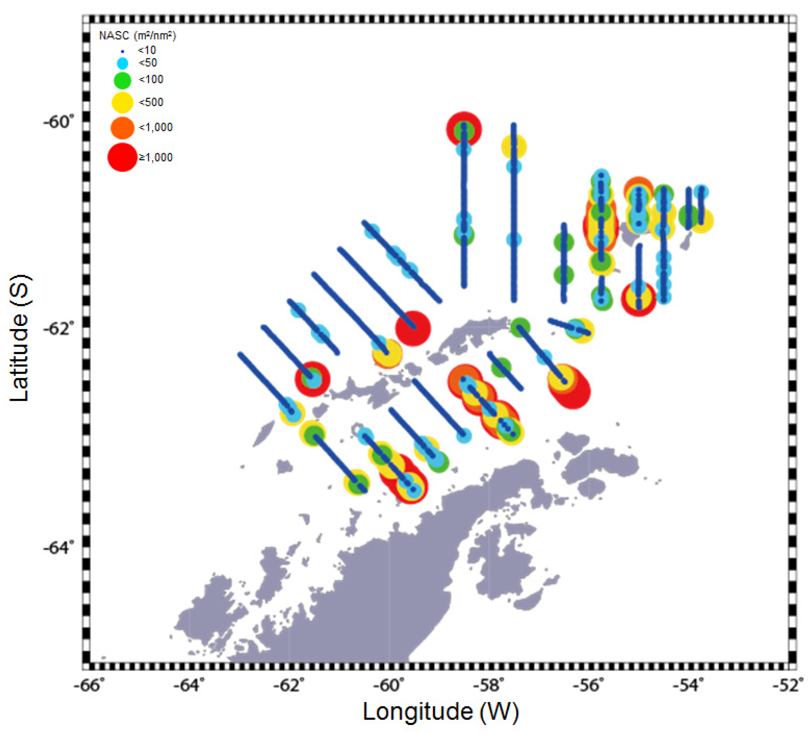
3.2. Spatiotemporal Distribution of Antarctic Krill

The density was Antarctic krill was noticeably higher in the South and Elephant Island areas, compared to its west area. The Antarctic krill showed a higher density at a depth of 200 m compared to all other depths (Figure 8).

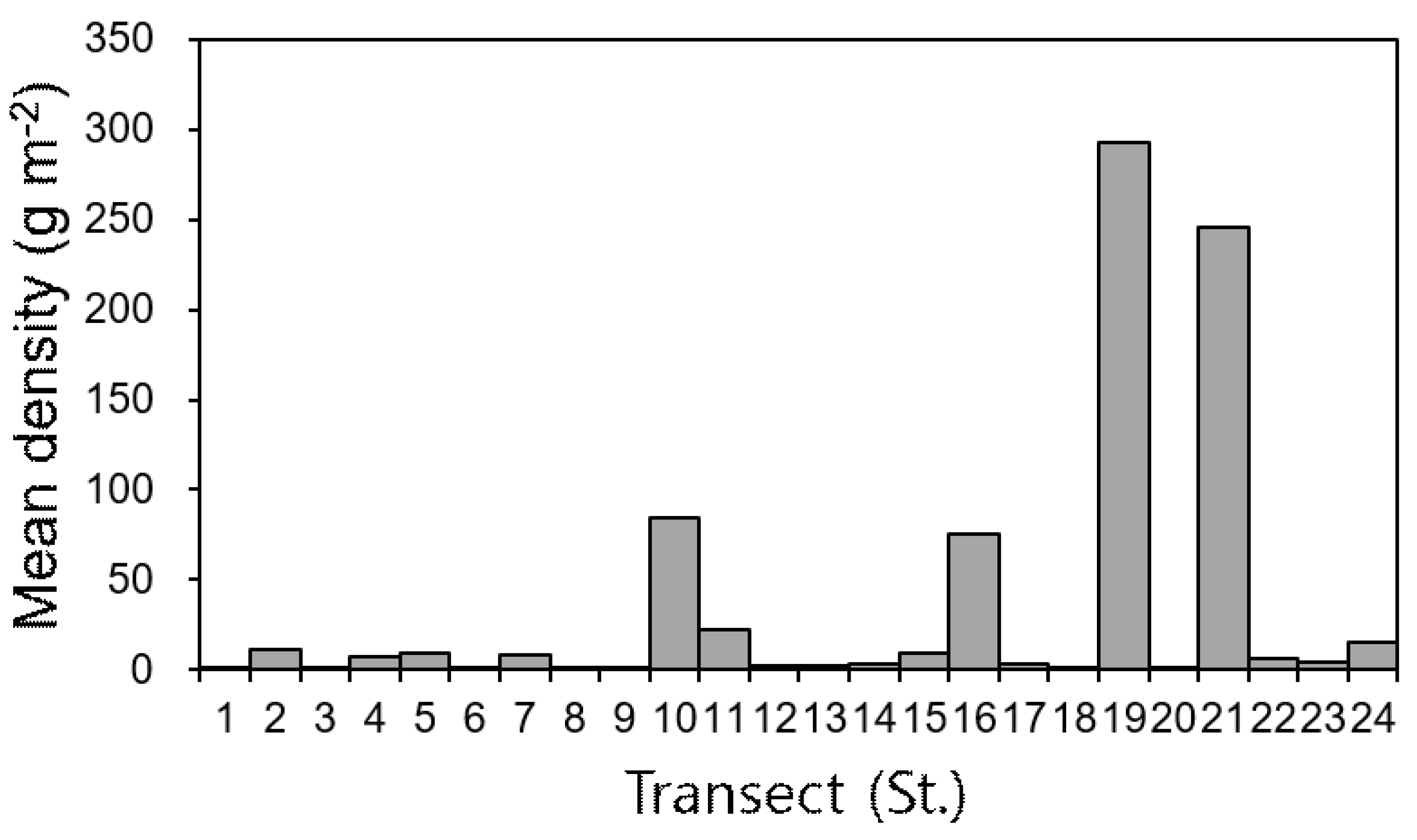
3.3. Density of Antarctic Krill

Figure 9 shows the mean Antarctic krill density along each survey line. The density of Antarctic krill was similar using either the TS or S_V values. Antarctic krill density was especially high at St. 19 and 21 in the South area, where the mean density was over 250 g m⁻². The mean Antarctic krill density across the survey area was 33.65 g m⁻² (CV = 45.97%).

4. Discussion

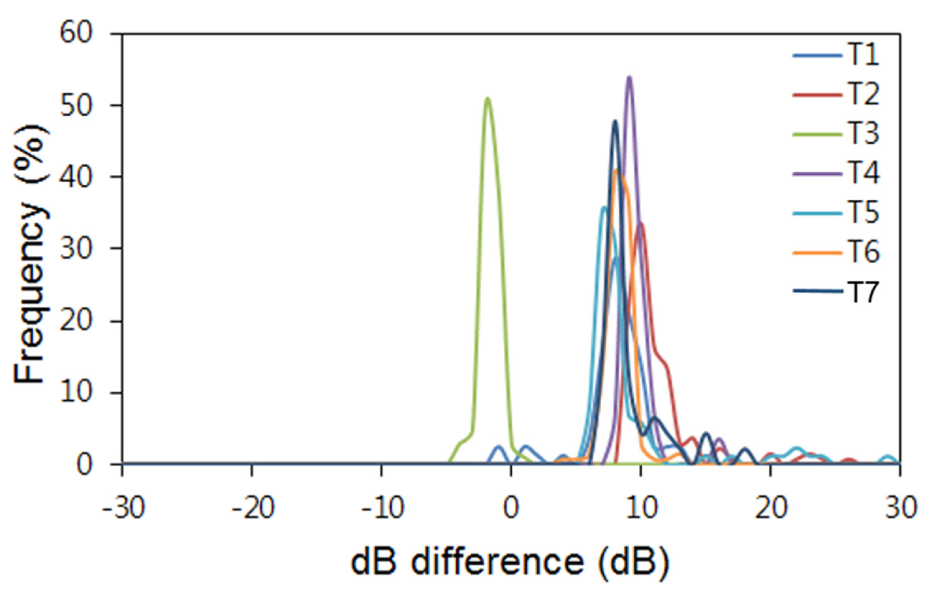
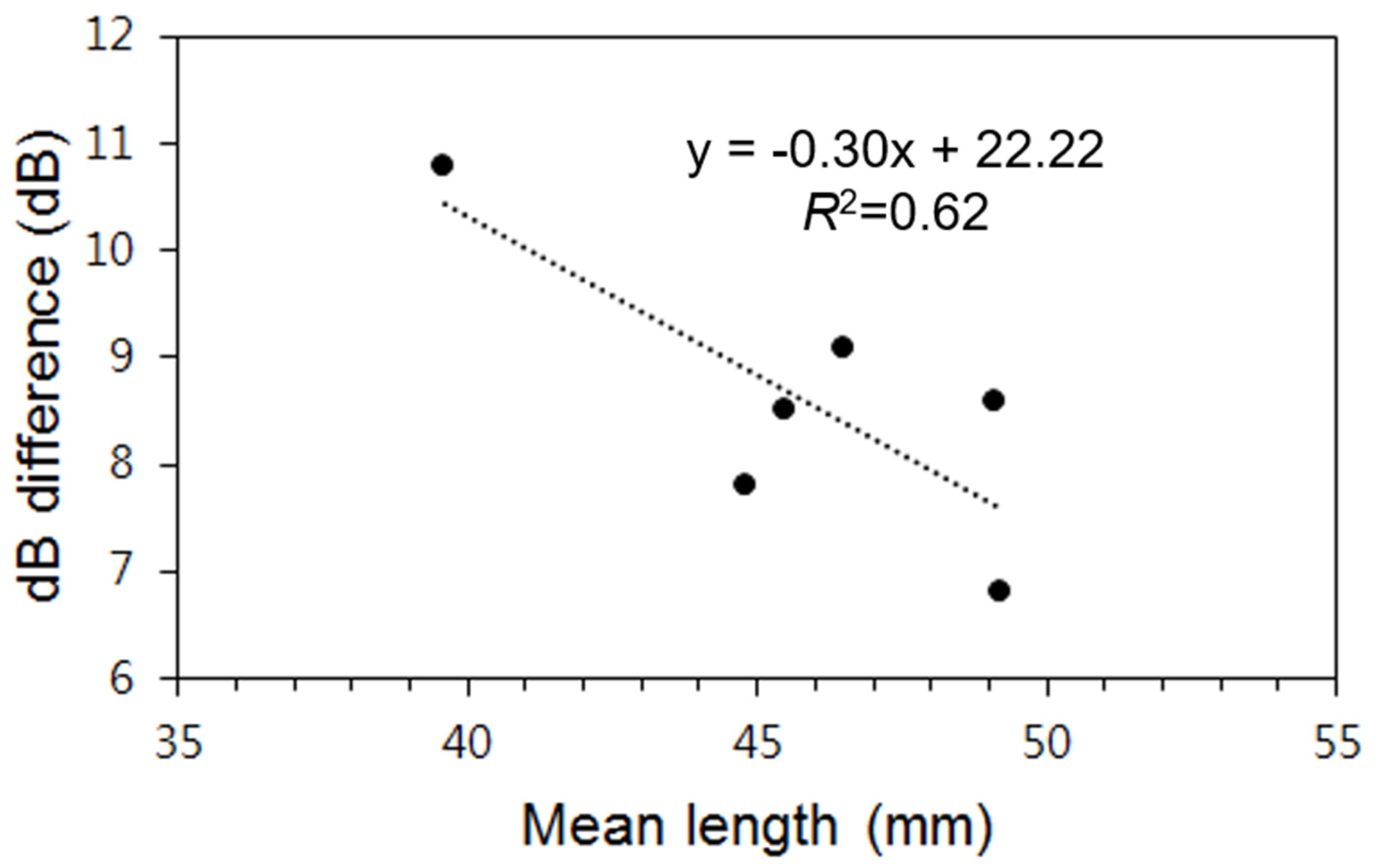
4.1. dB Differences of Antarctic Krill

In general, Antarctic krill are distinguished from other organisms using techniques based on dB differences [17,18]. In the present study, we used the S_V differences (0.4–13.4 dB) to isolate the Antarctic krill signal. Figure 10 shows the dB differences for each of the collected species from the different sampling points. Antarctic krill was dominant, constituting at least 99.9% of the catch, at all sampling points, except St. T3, where only E. carlsbergi was caught. The inter-frequency S_V differences (mean ± S.D.) were 6.8 ± 2.6 dB at St. T1, 10.8 ± 3.1 dB at St. T2, −2.1 ± 0.7 dB at St. T3, 9.1 ± 1.4 dB at St. T4, 8.6 ± 4.6 dB at St. T5, 7.8 ± 1.1 dB at St. T6, and 8.5 ± 2.4 dB at St. T7 (Figure 10). Thus, the S_V difference was not the same in waters where over 99.9% Antarctic krill was caught and waters where only E. carlsbergi was caught. In waters where Antarctic krill was caught, the inter-frequency S_V difference range (5–95%) was 6.5–11.1 dB, which is included in the dB differences used in this study.

The differences in the S_V difference ranges were strongly correlated with Antarctic krill size. The inter-frequency S_V difference varies with seasonal changes in Antarctic krill size, with the S_V difference tending to decrease as Antarctic krill size increases [19]. Likewise, in the present study we verified that the inter-frequency S_V difference decreased with increasing mean Antarctic krill size at each sampling point (Figure 11). Antarctic krill TS was calculated using a SDWBA model, with the TS difference (120–38 kHz) at 2–16 dB decreasing with increasing size [20].

When Kang et al. [21] collected samples from the Antarctic Peninsula using an Isaacs-Kidd Midwater Trawl (IKMT), in addition to Antarctic krill, they found amphipods, copepoda, and salps, with salps (Salpa thompsoni) constituting a particularly large proportion. In the field, the TS of Salpa thompsoni has been measured as −75.7, −74.2 dB at 38 kHz and −71.4, −71.1 dB at 120 kHz, meaning that there is no TS_{120-38 kHz} difference [22]. It is often difficult to distinguish salps from Antarctic krill because the dB differences (120–38 kHz) are similar. However, Neocalanus cristatus, which is a copepod species, has a mean ∆MVBS_{120-38 kHz} of 13.7–17.3 dB, and shows a large dB differences [23]. It should be possible to distinguish Antarctic krill from copepods, because the dB differences are distinct. Wiebe et al. [22] reported that zooplankton only have a small effect (<10%) on Antarctic krill abundance. However, because the sampling nets used in the present study were trawl nets used in commercial Antarctic krill fishing, small organisms were not collected. Therefore, to improve identify the species inhabiting the study area in the future, it will be necessary to use sampling tools for zooplankton.

4.2. Distribution and Density of Antarctic Krill

The density of Antarctic krill was noticeably high in the south area and near Elephant Island compared to the west area. The area near Elephant Island (to the east of Bransfield Strait) and the continental shelf north of the South Shetland Islands had steep gradients as the water became deeper (Figure 8) Elephant Island and north of the South Shetland Islands are locations where eddies form, leading to the formation of large populations of Antarctic krill, which move with the currents [21]. Previous studies reported a density contrast of Antarctic krill as 1.044 and 1.058 [24,25], confirming that they are heavier than seawater. Thus, it is thought that Antarctic krill have the ability to swim, in addition to being strongly affected by sea currents. Moreover, Antarctic krill are primarily found in coastal waters at a depth of around 200 m, with Ichii et al. [26] reporting that Antarctic krill form large groups along tidal fronts and in coastal regions.

The weighted density of Antarctic krill, along each survey line, was 0.1–109 g m⁻², with St. 19 and 21 in the South area containing particularly high densities of over 100 g m⁻². Kang et al. [27] previously showed that the density of Antarctic krill in the West and South areas was 44.9 g m⁻² and 30.3 g m⁻², respectively, while that near Elephant Island was 11.3 g m⁻². Reiss et al. [28] reported that the abundance of Antarctic krill was highest near Elephant Island and lowest in the south area. The mean density across the whole South Shetland Island area has been reported to be 37.7–58.3 g m⁻² [7,27].

5. Conclusions

This study was estimated through CCAMLR analytical methods to determine the distribution and density of Antarctic krill inhabiting the waters near the South Shetland Islands (Subarea 48.1) using acoustic. The density of Antarctic krill was 33.59 g m⁻² (CV = 45.97%) at S_{V120-38 kHz} range of 0.4–14.3 dB. The acoustic technology can be usefully used to estimate the density of Antarctic krill distributed over a wide area in short time.

References

1. Hewitt, R.; Demer, D.A. Dispersion and abundance of Antarctic krill in the vicinity of Elephant Island in the 1992 austral summer. Mar. Ecol. Prog. Ser. 1993, 99, 29–39. [Google Scholar] [CrossRef]
2. Everson, I. Distribution and standing, The Southern Ocean. In Krill Biology, Ecology and Fisheries; Everson, I., Ed.; Blackwell Science: New Jersey, NJ, USA, 2000; pp. 63–79. [Google Scholar]
3. Atkinson, A.; Siegel, V.; Pakhomov, E.A.; Jessopp, M.J.; Loeb, V. A re-appraisal of the total biomass and annual production of Antarctic krill. Deep Sea Res. Part I Oceanogr. Res. Pap. 2009, 56, 727–740. [Google Scholar] [CrossRef]
4. Jarvis, T.; Kelly, N.; Kawaguchi, S.; Wijk, E.; Nicol, S. Acoustic characterisation of the broad-scale distribution and abundance of Antarctic krill (Euphausia superba) off East Antarctica (30–80 E) in January–March 2006. Deep Sea Res. Part II Top. Stud. Oceanogr. 2010, 57, 916–933. [Google Scholar] [CrossRef]
5. Fielding, S.; Watkins, J.L.; Trathan, P.N.; Enderlein, P.; Waluda, C.M.; Stowasser, G.; Tarling, G.A.; Murphy, E.J. Interannual variability in Antarctic krill (Euphausia superba) density at South Georgia, Southern Ocean: 1997–2013. ICES J. Mar. Sci. 2014, 71, 2578–2588. [Google Scholar] [CrossRef]
6. Hewitt, R.P.; Linen Low, E.H. The fishery on Antarctic krill: Defining an ecosystem approach to management. Rev. Fish. Sci. 2000, 8, 235–298. [Google Scholar] [CrossRef]
7. Hewitt, R.P.; Watkins, J.; Naganobu, M.; Sushin, V.; Brierley, A.S.; Demer, D.; Brandon, M. Biomass of Antarctic krill in the Scotia Sea in January/February 2000 and its use in revising an estimate of precautionary yield. Deep Sea Res. Part II Top. Stud. Oceanogr. 2004, 51, 1215–1236. [Google Scholar] [CrossRef]
8. Lawson, G.L.; Wiebe, P.H.; Stanton, T.K.; Ashjian, C.J. Euphausiid distribution along the western Antarctic Peninsula. A. Development of robust multi-frequency acoustic techniques to identify euphausiid aggregations and quantify euphausiid size, abundance, and biomass. Deep Sea Res. II Top. Stud. Oceanogr. 2008, 55, 412–431. [Google Scholar] [CrossRef]
9. Cox, M.J.; Watkins, J.L.; Reid, K.; Brierley, A.S. Spatial and temporal variability in the structure of aggregations of Antarctic krill (Euphausia superba) around South Georgia, 1997–1999. ICES J. Mar. Sci. 2011, 68, 489–498. [Google Scholar] [CrossRef]
10. La, H.S.; Lee, H.; Kang, D.; Lee, S.; Shin, H.C. Volume backscattering strength of ice krill (Euphausia crystallorophias) in the Amundsen Sea coastal polynya. Deep Sea Res. Part II Top. Stud. Oceanogr. 2016, 123, 86–91. [Google Scholar] [CrossRef]
11. Fielding, S.; Cossio, A.; Cox, M.; Reiss, C.; Skaret, G.; Demer, D.; Watkins, J.; Zhao, X. A condensed history and document of the method used by CCAMLR to estimate krill biomass (B0) in 2010. In Proceedings of the CCAMLR WG-EMM-16/38, Hobart, Australia, 4–15 July 2016; Available online: https://www.ccamlr.org/en/wg-emm-16/38 (accessed on 7 July 2020).
12. Foote, K.G. Calibration of Acoustic Instruments for Fish Density Estimation: A Practical Guide; International Council for the Exploration of the Sea: Copenhagen, Denmark, 1987. [Google Scholar]
13. De Robertis, A.; Higginbottom, I. A post-processing technique to estimate the signal-to noise ratio and remove echosounder background noise. ICES J. Mar. Sci. 2007, 64, 1282–1291. [Google Scholar] [CrossRef] [Green Version]
14. Wang, X.; Zhao, X.; Zhang, J. A noise removal algorithm for acoustic data with strong interference based on post-processing techniques. In Proceedings of the CCAMLR SG-ASAM-15/02, Hobart, Australia, 9–13 March 2015; pp. 17–30. Available online: https://www.ccamlr.org/en/system/files/science_journal_papers/Wang%20et%20al.pdf (accessed on 7 July 2020).
15. Echoview. Available online: http://www.echoview.com/ (accessed on 13 June 2016).
16. Jolly, G.M.; Hampton, I. A stratified random transect design for acoustic surveys of fish stocks. Can J. Fish. Aquat. Sci. 1990, 47, 1282–1291. [Google Scholar] [CrossRef]
17. Hewitt, R.P.; Watkins, J.L.; Naganobu, M.; Tshernyshkov, P.; Brierley, A.S.; Demer, D.A.; Kasatkina, S.; Brandon, M.A. Setting a precautionary catch limit for Antarctic krill. Oceanography 2002, 15, 26–33. [Google Scholar] [CrossRef] [Green Version]
18. Conti, S.G.; Demer, D.A. Improved parameterization of the SDWBA for estimating krill target strength. ICES J. Mar. Sci. 2006, 63, 928–935. [Google Scholar] [CrossRef] [Green Version]
19. Fielding, S.; Watkins, J.; Cossio, A.; Reiss, C.; Watters, G.; Calise, L.; Skaret, G.; Takao, Y.; Zhao, X.; Agnew, D.; et al. The ASAM 2010 assessment of krill biomass for area 48 from the Scotia Sea. In Proceedings of the CCAMLR 2000 synoptic survey, CCAMLR WG-EMM-11/20, Hobart, Australia, 11–22 July 2011; Available online: https://www.ccamlr.org/en/wg-emm-11/20 (accessed on 7 July 2020).
20. Demer, D.A.; Conti, S.G. New target-strength model indicates more krill in the Southern Ocean. ICES J. Mar. Sci. 2005, 62, 25–32. [Google Scholar] [CrossRef]
21. Kang, D.H.; Hwang, D.J.; Kim, S.A. Biomass and distribution of Antartic Krill, Euphausia superba, in the Northern part of the South Shetland Island, Antarctic Ocean. Kor. J. Fish. Aquat. Sci. 1999, 32, 737–747, (in Korean with English abstract). [Google Scholar]
22. Wiebe, P.H.; Chu, D.; Kaartvedt, S.; Hundt, A.; Melle, W.; Ona, E.; Batta-Lona, P. The acoustic properties of Salpa thompsoni. ICES J. Mar. Sci. 2009, 67, 583–593. [Google Scholar] [CrossRef] [Green Version]
23. Murase, H.; Ichihara, M.; Yasuma, H.; Watanabe, H.; Yonezaki, S.; Nagashima, H.; Miyashita, K. Acoustic characterization of biological backscatterings in the Kuroshio-Oyashio inter-frontal zone and subarctic waters of the western North Pacific in spring. Fish. Oceanogr. 2009, 18, 386–401. [Google Scholar] [CrossRef]
24. Greenlaw, C.F. Acoustical estimation of zooplankton populations 1. Limnol. Oceanogr. 1979, 24, 226–242. [Google Scholar] [CrossRef]
25. Becker, K.N.; Warren, J.D. Material properties of Northeast Pacific zooplankton. ICES J. Mar. Sci. 2014, 71, 2550–2563. [Google Scholar] [CrossRef] [Green Version]
26. Ichii, T.; Katayama, K.; Obitsu, N.; Ishii, H.; Naganobu, M. Occurrence of Antarctic krill (Euphausia superba) concentrations in the vicinity of the South Shetland Islands: Relationship to environmental parameters. Deep Sea Res. Part I Oceanogr. Res. Pap. 1998, 45, 1235–1262. [Google Scholar] [CrossRef]
27. Kang, D.H.; Shin, H.C.; Lee, Y.H.; Kim, Y.S.; Kim, S.A. Acoustic estimate of the krill (Euphausia superba) density between south Shetland islands and south Orkney islands, Antarctica, during 2002/2003 Austral summer. Ocean Polar Res. 2005, 27, 75–86, (in Korean with English abstract). [Google Scholar]
28. Reiss, C.S.; Cossio, A.M.; Loeb, V.; Demer, D.A. Variations in the biomass of Antarctic krill (Euphausia superba) around the South Shetland Islands, 1996–2006. ICES J. Mar. Sci. 2008, 65, 497–508. [Google Scholar] [CrossRef] [Green Version]
Figure 1. Survey lines and sampling points for acoustic and net surveys to determine the density of Antarctic krill.
Sustainability 12 05701 g001
Figure 2. Flowchart for noise removal from the acoustic data.
Sustainability 12 05701 g002
Figure 3. Example echogram after noise removal from the acoustic data. Raw echogram with noise (a), copied raw echogram after applying TVT (Time Varied Threshold) (b), eliminate noise smaller than the minimum volume backscattering strength (SV) of Antarctic krill and larger than the maximum SV of Antarctic krill (c), echogram applied the erosion filter 3 × 3 (d), echogram applied the dilation filter 5 × 5 and 5 × 5 (e,f), echogram applied the median filter 7 × 7 (g), and echogram selected noise eliminated (h).
Sustainability 12 05701 g003
Figure 4. Flowchart for processing the dB differences for Antarctic krill at 38 and 120 kHz [15].
Sustainability 12 05701 g004
Figure 5. Catch per unit effort (CPUE) of Antarctic krill catches by trawling.
Sustainability 12 05701 g005
Figure 6. Size distribution of Antarctic krill caught in the trawl, by sampling site of St. 1 (a), St. 2 (b), St. 5 (c), St. 5 (d), St. 6 (e), St. 7 (f).
Sustainability 12 05701 g006
Figure 7. Size distribution of Antarctic krill caught across all sampling points (n = 1200).
Sustainability 12 05701 g007
Figure 8. Spatiotemporal distribution of Antarctic krill using the minimum volume backscattering strength (Sv) differences of between 120 and 38 kHz (0.4 < ∆MVBS120-38 kHz < 14.3 dB).
Sustainability 12 05701 g008
Figure 9. Density of Antarctic krill populations along each survey line SV difference between 120 and 38 kHz (0.4 < ∆MVBS120-38 kHz < 14.3 dB).
Sustainability 12 05701 g009
Figure 10. Comparison of inter-frequency SV differences among trawl sampling points.
Sustainability 12 05701 g010
Figure 11. Relationship between Antarctic krill size and dB differences at each trawl sampling site.
Sustainability 12 05701 g011