Article

Environmental Justice in The Netherlands: Presence and Quality of Greenspace Differ by Socioeconomic Status of Neighbourhoods

1
Cultural Geography/Wageningen Environmental Research, Wageningen University & Research, P.O. Box 47, 6700 AA Wageningen, The Netherlands
2
Forest and Nature Policy/Wageningen Environmental Research, Wageningen University & Research, P.O. Box 47, 6700 AA Wageningen, The Netherlands
3
Wageningen Environmental Research, Wageningen University & Research, P.O. Box 47, 6700 AA Wageningen, The Netherlands
*
Author to whom correspondence should be addressed.
Sustainability 2020, 12(15), 5889; https://0-doi-org.brum.beds.ac.uk/10.3390/su12155889
Submission received: 3 July 2020 / Revised: 10 July 2020 / Accepted: 20 July 2020 / Published: 22 July 2020
(This article belongs to the Special Issue Green Urban Development)

Abstract

:
Making our cities more sustainable includes the need to make the transition a just one. This paper focuses on distributive justice with regard to greenspace in cities. Urbanisation and densification will likely result in less greenspace in urban residential areas, especially in deprived neighbourhoods. This is a threat to the aim of healthy and liveable cities, as greenspace has positive effects on human health and well-being. In this study, we show that in The Netherlands, neighbourhoods with a low socioeconomic status already tend to have a lower presence and quality of greenspace than those with a high socioeconomic status. This outcome is independent of the greenness metric that was used. However, depending on the precise greenness metric, socioeconomic differences in greenness between neighbourhoods are smaller in highly urban municipalities than in less urban municipalities, rather than larger. The paper discusses the implications of these outcomes for policy and planning regarding urban greenspace.

1. Introduction

Current debates on sustainable cities not only focus on a transition towards greener cities, but also on the need to make this transition a just one. For example, the recently published European Green Deal recognises that environmental justice is key for a successful transition towards sustainable cities. This Green Deal “aims to protect, conserve and enhance the EU’s natural capital, and protect the health and well-being of citizens from environment-related risks and impacts. At the same time, this transition must be just and inclusive” [1] (p. 2). Environmental justice can be conceptualised as distributive, procedural and recognitional justice [2]. According to the World Health Organization, distributive justice refers to the spatial distribution of environmental risks and amenities and the resulting disparities among socioeconomic and racial groups [3]. In this study, we focus on distributive justice regarding urban greenspace, more specifically on socioeconomic differences in the presence and quality of greenspace in residential environments in The Netherlands. Our reason for doing so is based on a combination of factors.
To begin with, the world’s population is rising, and growing numbers will be housed in cities. An important element of this urbanisation is the densification of cities. In line with global trends, although already heavily urbanised, The Netherlands is also expected to further densify its cities. Based on prognoses, its national government foresees a need for 700,000 new dwellings by the year 2025 [4]. Furthermore, it has decided that in principle these new dwellings should be realized within the existing urban fabric. Although compact cities may have some advantages, even with regard to certain health aspects [5,6], densification is likely to lead to less open space being available, certainly on a per capita basis [7,8]. This includes green open space, such as urban parks and domestic gardens. At the same time, providing universal access to safe, inclusive and accessible, green and public spaces is one of the targets of the UN’s Sustainable Development Goal 11: to make cities and human settlements inclusive, safe, resilient and sustainable (target 11.7) [9]. The relevance of this target is supported by mounting evidence for a positive effect of the presence of and contact with nature on human health and well-being [10,11,12,13,14]. This effect appears to be even stronger for people with a low socioeconomic status (SES) and/or living in deprived neighbourhoods. Examples of studies showing this are Brown et al. (USA) [15], Cusack et al. (USA) [16], Balseviciene et al. (Latvia) [17], Markevych et al. (Germany) [18], Xu et al. (China) [19] and Maas et al. [20], De Vries et al. [21], Groenewegen et al. [22] (all The Netherlands). Therefore, we consider it relevant to assess the presence and quality of greenspace in Dutch residential neighbourhoods, and whether this differs by the socioeconomic status of those neighbourhoods.

1.1. Previous Studies on Inequalities in Access to Greenspace

Recently, the distributive justice issue of unequal presence of greenspace has started to be highlighted [23]. For example, Landry and Chakraborty evaluated the spatial distribution of public right-of-way trees in Florida and observed a significantly lower proportion of tree cover in neighbourhoods containing a higher proportion of low-income residents [24]. In the Netherlands, Kruize et al. investigated the disparities in the availability of public greenspace across socioeconomic status in the highly urban Rijnmond Region [25]. They found that the higher-income groups within this region generally had better access to environmental amenities, especially to public greenspace, while the lower-income groups lived in places with somewhat lesser environmental quality. More recently, Schüle and others concluded that this was also the case in several other European countries [26]. However, high-income groups do not always have more greenspace nearby. Vaughan et al. conducted research on the distribution of park availability, features, and quality across income levels in Kansas City, Missouri. They found that the population of low-income neighbourhoods shared more parks. However, these were parks of a low quality. The parks of medium-income neighbourhoods contained more aesthetic features per park. The high-income neighbourhoods enjoyed more parks with basketball courts, but fewer parks with trails [27]. So, in addition to the amount of greenspace, environmental injustice may also occur in terms of the quality of greenspace. Therefore, ideally distributive environmental justice in this case implies that everybody has equal access to good quality greenspace.

1.2. Research Questions

In this study, we will look at socioeconomic inequality in the distribution of greenspace in the Netherlands. We aim to extend the earlier research by Kruize et al. [25] from 2007 in several ways. To begin with, we will explore the robustness of the phenomenon by comparing results for different greenness metrics, including quality-based metrics. We will also look at different ways to characterize the socioeconomic status of a neighbourhood. Secondly, we will not only look at highly urban neighbourhoods, but also at less urban neighbourhoods. Much of the research on (differences in) the presence of greenspace focuses on highly urban environments. Presumably, this is partially based on the assumption that socioeconomic differences in presence are likely to be more pertinent in environments were greenspace is scarce (and therefore having it nearby may be expensive). In our study, we will explore whether socioeconomic differences in presence indeed vary by level of urbanity. To summarize, our research questions are:
  • Is the presence and quality of greenspace in residential environments in the Netherlands related to the socioeconomic status of the neighbourhood?
  • To what extent do such differences depend on the specific socioeconomic characteristic and/or the greenness metric that is used to characterize the neighbourhood?
  • Do the above differences, if present, vary by the level of urbanity of the municipality in which the neighbourhood is located?

2. Materials and Methods

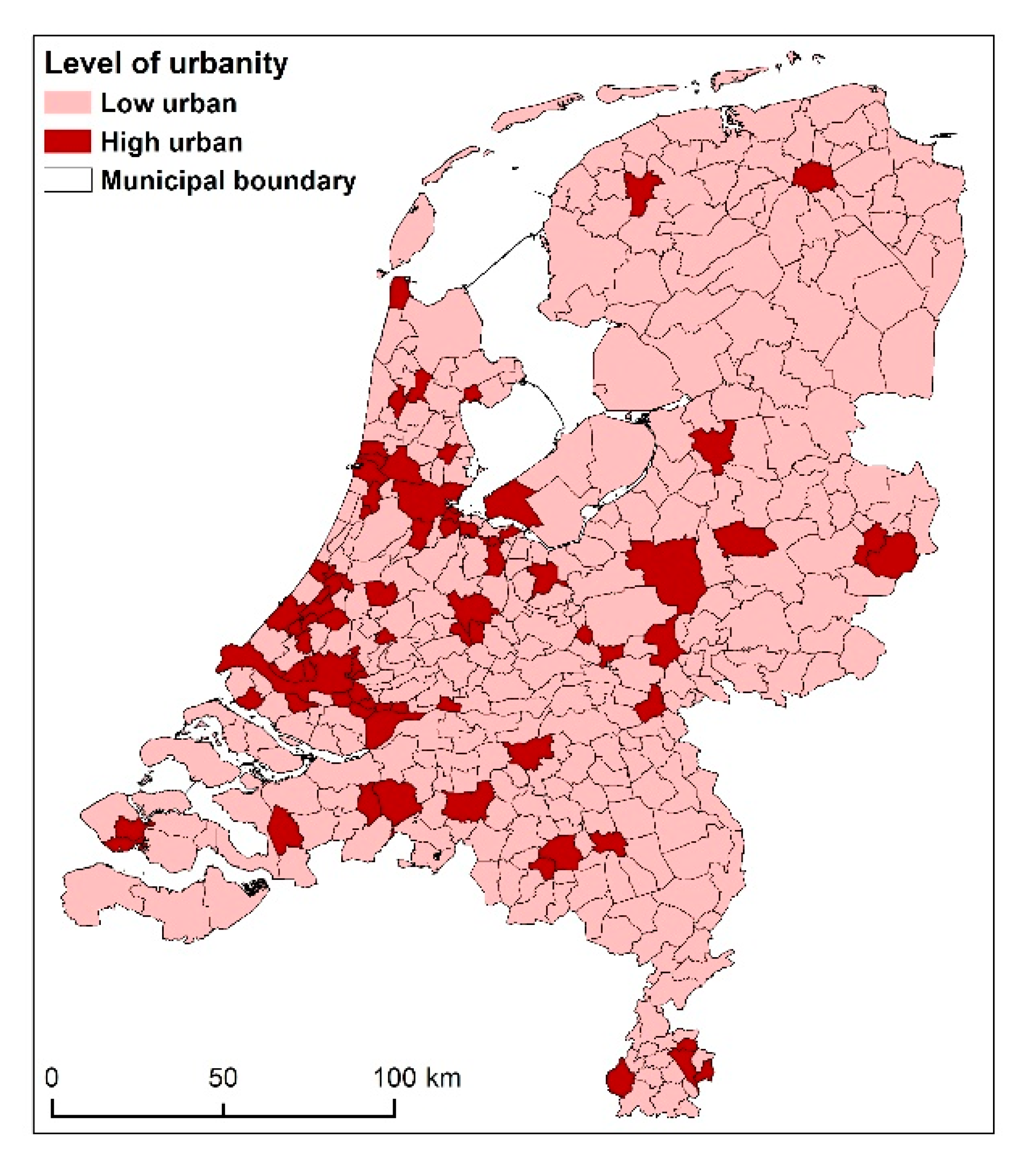
2.1. Neighbourhoods, Their Socioeconomic Classification and Level of Urbanity

Within this study, the neighbourhood is used as unit of observation, because it is the smallest spatial unit on which socioeconomic information is publicly available nationwide. We used data from 2012, because this was the most recent year for which data were available for all greenness metrics we thought to be of interest. Neighbourhoods are administrative units with boundaries decided upon by municipal authorities. In 2012, The Netherlands was divided into 12,001 neighbourhoods. They had an average size of about 300 ha (land only), with sizes being smaller in urban areas and larger in rural areas. The average population size was about 1400 people, with larger populations in urban areas and smaller ones in rural areas.
We classified neighbourhoods according to their socioeconomic status based on three different characteristics:
  • Percentage of households with a low annual income;
  • Percentage of households with a high annual income;
  • Average residential property value.
All three characteristics are based on the ‘Key figures for neighbourhoods’ database from Statistics Netherlands (in Dutch: Centraal Bureau voor de Statistiek, or CBS) for the year 2012 [28]. A low-income household was defined by CBS as a household with an annual disposable income of 25,100 euro at maximum; this is about 40% of all households. Neighbourhoods are separated into three categories: neighbourhoods where low-income households comprise a maximum of 30% of all households, those where that figure is between 30% and 50%, and finally those where at least 50% of all households are designated as low-income. Note that a high percentage of low-income households signifies a low socioeconomic status of the neighbourhood.
A high-income household is defined by CBS as a household with an annual disposable income above 46,500 euro; this is about 20% of all households. Furthermore, for this characteristic, neighbourhoods are separated into three categories: neighbourhoods where high-income households comprise a maximum of 20% of all households, those where that figure is between 20% and 35%, and finally those where at least 35% of all households are designated as high-income. Finally, the average residential property value is based on the Valuation of Immovable Property Act (Dutch acronym: WOZ). All owners of real estate pay real estate tax based on the WOZ value in Netherlands. The WOZ value is also separated into three categories: ≤ 200, 200–300, and ≥ 300 (all * 1000 euro).
An additional variable that is used in this study is the level of urbanity of the municipality to which the neighbourhood belongs. As mentioned before, we wanted to investigate whether the relationship between socioeconomic status and greenness differs between cities and small towns/the countryside. The data for urbanity are likewise taken from Statistics Netherlands (CBS). Urbanity is based on address density and is presented by CBS in five classes, from very strongly urban to not urban. In our analyses we combined very strongly urban and strongly urban, as well as moderately, weakly urban and not urban. A density above 1500 addresses per km2 is defined as highly urban and densities below this value as signifying a low level of urbanity. Of all neighbourhoods, 32% are located in a high-urban municipality and 68% in a low-urban municipality (see Figure 1).

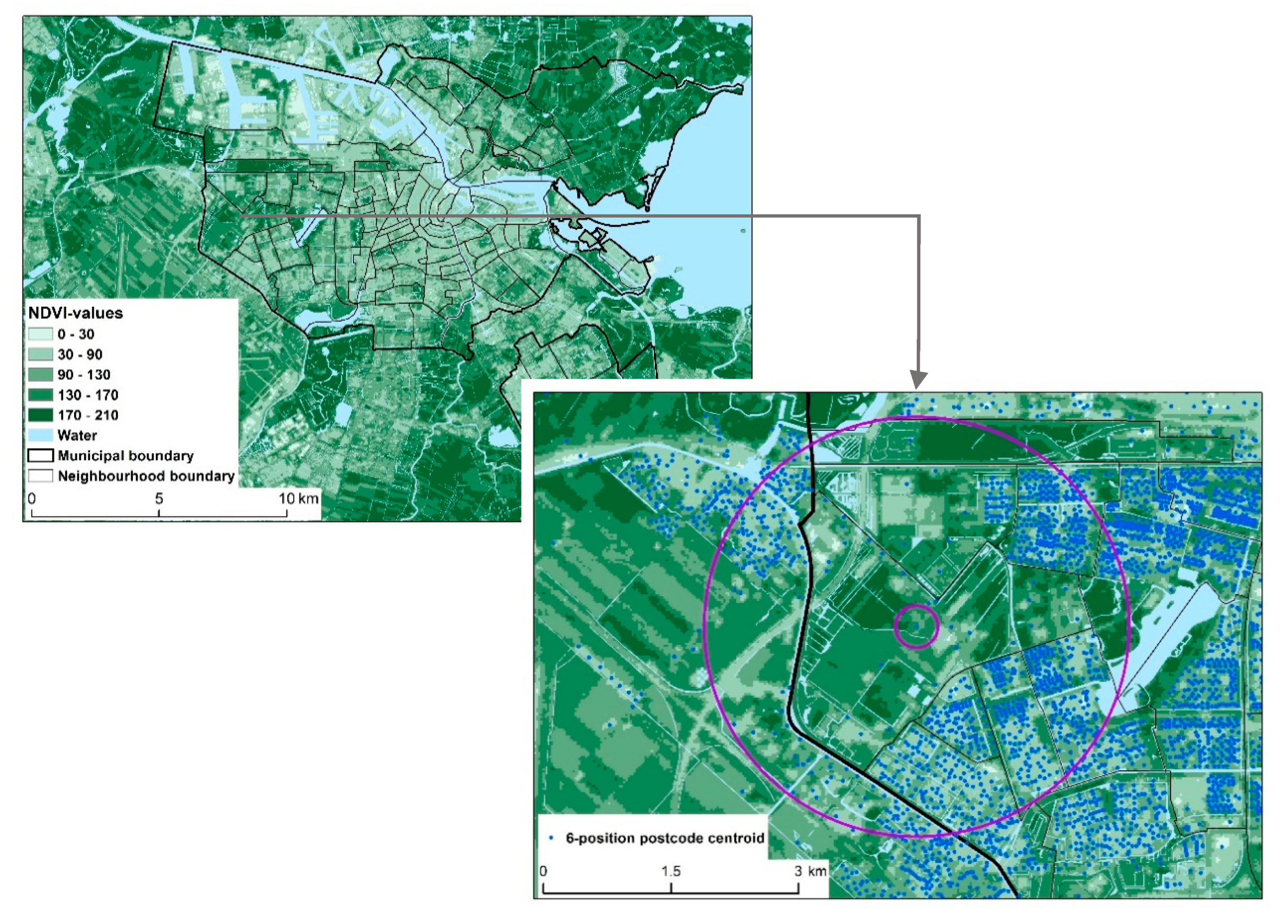
2.2. Types of Greenness Metrics and Buffer Sizes

One of the reasons we chose to look into distributive justice issues specifically with regard to greenspace is its association with human health and well-being. Most of the epidemiological studies on this topic focus on greenspace in the residential environment. However, they have used different definitions of greenspace and of its accessibility. In their narrative review, Ekkel and de Vries distinguish two categories of access metrics: cumulative opportunity metrics and residential proximity metrics [29]. The first category focuses on the total amount of greenery or greenspace that is present within a certain area, or distance from home. The second category focuses on the distance to the nearest green area that satisfies certain criteria, usually having at least a minimum size and being open to the public. Ekkel and de Vries tentatively conclude that cumulative opportunity metrics are more consistently related to health indicators. Therefore, in this study we will focus on this type of metric and look at two commonly used cumulative opportunity metrics: the percentage of green land use in the residential environment and its average score on the Normalized Difference Vegetation Index (NDVI) [29].
We calculated the percentage of green land use in the residential environment based on the National Land Cover Classification database (LGN7), which contains the dominant type of land use of each 25 × 25 m grid cell for the whole of The Netherlands for the year 2012 [30]. Several categories of land use were combined to arrive at the total amount of greenspace, following Maas et al. [20]: urban greenspaces (e.g., parks), agricultural areas, forests and nature areas. Focusing on a buffer around the midpoint of every 6-digit postcode area in the Netherlands (containing about 15 households on average), we determined the percentage of the area covered by greenspace. Since a range of different buffer sizes are used in the greenspace health literature, without it being clear which size is to be preferred [31,32,33], we applied two buffer sizes: a rather small one (250 m) and a relatively large one (2.5 km). The data were aggregated to the neighbourhood level by calculating the average percentage over all 6-digit postcodes within a neighbourhood. Since the density of postcodes indicates where most people live within the neighbourhood, the average score of all 6-digit postcodes in the neighbourhood constitutes approximately a population-weighted neighbourhood mean.
The Normalized Difference Vegetation Index (NDVI) indicates the presence of green biomass, based on the ratio of near infrared and red light [34]. The NDVI approach differs from the land-use approach in that small green elements, such as street trees and domestic gardens, also contribute. Furthermore, different types of greenery result in different NDVI scores. For example, woodlands (when in leaf) tend to score higher than grassy areas. NDVI assessments are based on satellite imagery, in this case on LANDSAT5 data for 25 May and 25 July 2012, both cloud-free days. The average of the NDVI scores for these two days was used. In principle, the NDVI score is unitless and ranges from minus one (−1) to plus one (+1). We re-scaled the scores. For convenience, the original scores above 0 were multiplied by 250. All original scores below or equal to 0 (indicating an absence of green biomass, which may include surface waters) were given a new score of 1, to prevent blue space (water) and greenspace from cancelling each other out. Subsequently, scores were aggregated to the neighbourhood level in two steps. In the first step, mean NDVI values were calculated for the same two distances (buffers) around each 6-digit postcode as before. In the second step, the average of these means was calculated over all 6-digit postcodes within a neighbourhood (see Figure 2).
Specifically, for this study, we developed an additional metric to assess the presence of small green elements within predominantly built-up areas, the NDVI-B (B for built-up area). As mentioned before, small green elements also contribute to the NDVI score. However, the average score for a buffer is likely to be dominated by green areas. We developed the NDVI-B to be more complementary to the percentage of greenspace, whereas the regular NDVI score is likely to correlate rather highly with this percentage, since green land uses by definition imply higher NDVI values. The NDVI-B score is calculated in the same way as the previous NDVI score, but now only for the built-up area within the buffer. The same land-use database that was used to determine the percentage of greenspace (LGN7) is used to determine the built-up area within the different buffers: all types of land use that are not green or blue (water). The mean NDVI-B score is calculated for the same two buffer sizes, 250 m and 2.5 km, and subsequently averaged per neighbourhood.
As for relevant qualities of greenspace, the scientific literature offers less information, presumably for two reasons. The first reason is that it is not yet known which characteristics of greenspace are the most relevant with regard to human health and well-being [10,11,12,13,14]. As with different buffer sizes, this may depend on the pathway linking greenspace with health, as well as on the particular health aspect at hand. The second reason is that it is more difficult to gather large-scale data on quality aspects. Whereas quantity and distance information on greenspace usually is acquired by making use of remote sensing and geographical databases, this tends not to be an option for more detailed information on its qualities. The costs of acquiring quality information by site visits quickly become prohibitively high. However, based on existing models in The Netherlands, we will look at two quality aspects.
The first quality aspect deals with the peace and quiet that may be experienced during visits to nearby greenspaces. Given that stress reduction is an important pathway linking greenspace and health [35], this is likely to be a relevant quality aspect with regard to well-being effects. The metric is based on the amount of greenspace that is locally available, in relation to the number of people that may be expected to visit this greenspace for recreational purposes. The lower the availability per person, the less peace and quiet is likely to be experienced during a visit. Thus, in contrast to the previous metrics, this metric not only looks at the amount of greenspace, but takes the size of the local demand for greenspace into account, specifically the demand for walking in a natural environment. Green land uses are assigned a capacity in terms of the number of people they can accommodate per hectare per day. This capacity is high for urban parks and forests and low for agricultural areas, especially if the path density in the latter is low and its visual openness is high (one can oversee a large area at one glance). Subsequently, the available capacity is distributed over the neighbourhoods, having their midpoint within a distance of 2.5 km of the green area, proportionally to the size of the demand originating from the different neighbourhoods within this distance. The outcome is the capacity assigned to a neighbourhood, expressed as a percentage of the capacity that is needed to fully satisfy the demand originating from that neighbourhood. Within the model, a neighbourhood is not allowed to receive more capacity than it needs; therefore, the maximum value of this metric is 100%. Values below 100% are indicative of shortages. The model, called AVANAR, has been described in more detail elsewhere [36]. Its outcomes have been shown to be related to recreational behaviour [37,38]. In this study, supply data are mainly from 2008 and demand data from 2012 (see Figure 3).
The second quality aspect is about the scenic beauty of the greenspace. More beautiful areas are likely to attract more visits; plus, visits of such areas may be expected to lead to more pleasurable experiences, resulting in a more positive effect on one’s mood [39]. This metric is based on a model that predicts the average scenic beauty score that Dutch people assign to the countryside surrounding their place of residence, the GIS-based Landscape Appreciation Model (GLAM). Its predictions are based on four indicators: naturalness, historical character, nearby urban development and skyline disturbance. Each indicator itself is based on data on physical characteristics of the landscape. GLAM is described in more detail elsewhere, and has been validated [40]. In this study, version 2 of GLAM is used, with the main data from 2009. GLAM produces predictions for each 250 × 250 grid cell of countryside. We calculated the average value for all grid cells of countryside within a 2.5 km buffer for each (6-position) postcode, the same buffer size as used for the AVANAR model. Likewise, in a second step these values are averaged over all postcodes within a neighbourhood.
To summarize, eight greenspace metrics are used to characterise neighbourhoods, three of which for a 250 m buffer:
  • percentage of greenspace, averaged over 6-digit postcodes—scale: 0–100;
  • NDVI score, averaged over 6-digit postcodes—scale: 1–250;
  • NDVI score for the built-up area only (NDVI-B), averaged over 6-digit postcodes—scale: 1–250;
and five of which for a 2.5 km buffer:
  • percentage of greenspace, averaged over 6-digit postcodes—scale: 0–100;
  • NDVI score, averaged over 6-digit postcodes—scale: 1–250;
  • NDVI score for the built-up area (NDVI-B), averaged over 6-digit postcodes—scale: 1–250;
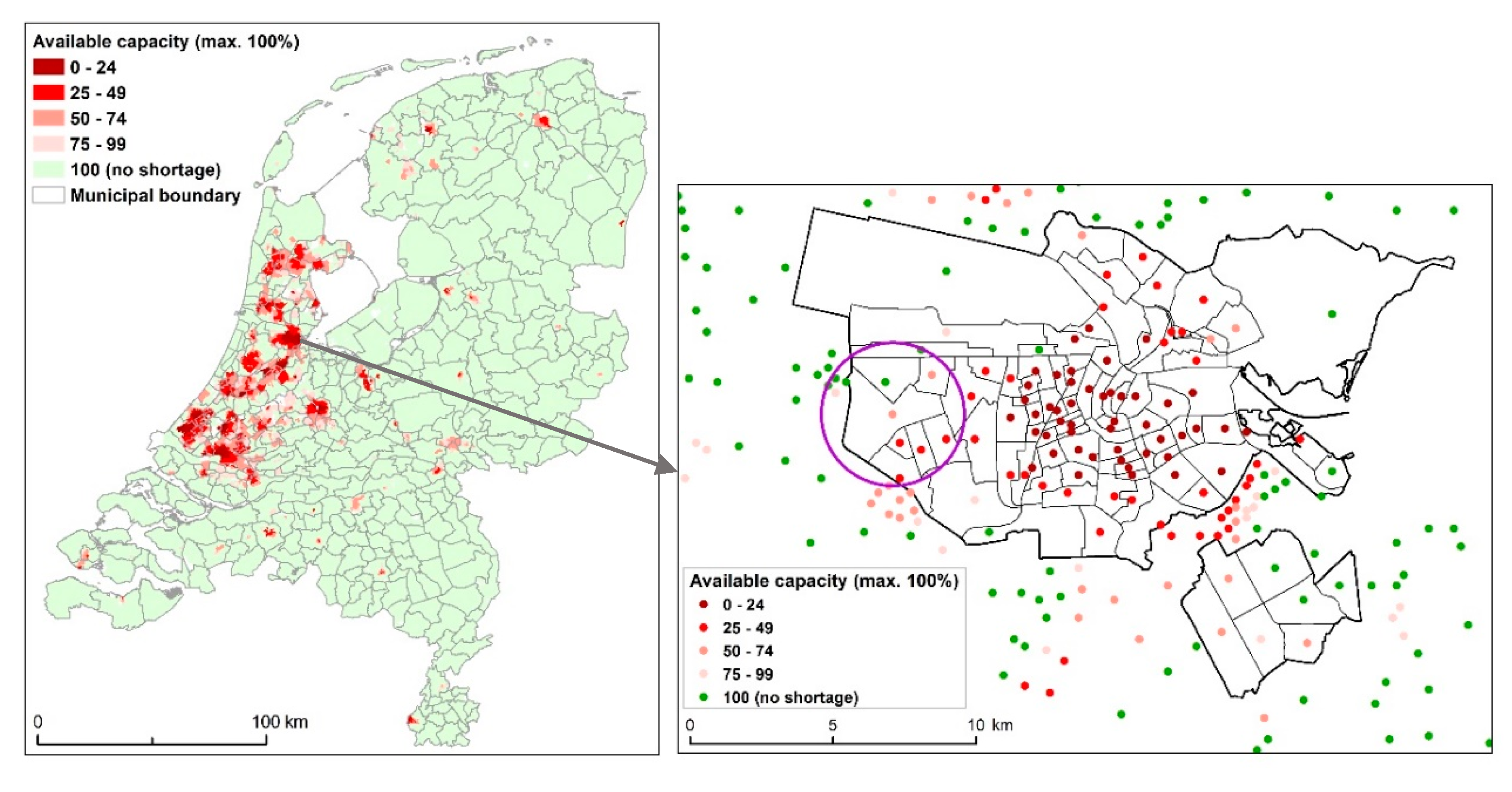
  • percentage of the demand for opportunities for recreational walks in a green environment that is satisfied by the local supply—scale: 0–100;
  • average predicted scenic beauty of the countryside—scale: 1–10.

2.3. Analysis

In all analyses, neighbourhoods are the units of observation. As a first step in the analysis, we look at the bivariate Pearson correlations among the eight greenspace metrics, as well as those among the three socioeconomic metrics. Pearson correlations are a measure of covariation, more specifically for the extent to which two variables are linearly related. If bivariate correlations are very high, then there is less need to conduct all possible analyses resulting from crossing each socioeconomic metric, as independent variable, with each greenspace metric, as dependent variable. The most redundant metrics will be discarded for further analysis.
As mentioned before, each socioeconomic metric is binned into three classes: low, middle and high. To assess differences in presence of greenspace between socioeconomic classes, separate analyses of variance are conducted for each combination of a remaining socioeconomic classification as independent variable (factor) and a remaining greenness metric as dependent variable. Analysis of variance (ANOVA) is a common statistical method to test whether groups have different means for the dependent variable. It is based on comparing the between-group variation (differences between group means) with the within-group variation. The first factor defining groups is one of the socioeconomic classifications. Since we are interested in whether socioeconomic differences in greenspace presence vary by the level of urbanity of the municipality (high or low), level of urbanity constitutes a second factor in the ANOVA. However, our interest is not in differences in greenspace presence or quality by level of urbanity as such, but in whether or not differences between socioeconomic categories vary by level of urbanity of the municipality. Therefore, the design of the analysis also includes the two-way interaction between the socioeconomic class of the neighbourhood and the level of urbanity of the municipality to which it belongs.

3. Results

Table 1 shows the size of the three classes for each of the three socioeconomic characteristics, overall as well as by level of urbanity. Note that for the percentage of low-income households, few low incomes indicate a high socioeconomic status. Income data are more frequently missing than data on residential property value. Furthermore, note that for the low-income metric the category with the highest percentage of low incomes was chosen rather extreme, containing a low share of all neighbourhoods (16.4%). In other words, for the percentage of low-income households this category contains the very poor neighbourhoods. Conversely, for the percentage of high-income households the highest category contains the very wealthy neighbourhoods (15.6%).
The distribution of neighbourhoods over the three classes per socioeconomic characteristic differs by municipal level of urbanity. In high-urban municipalities, neighbourhoods with many low-income households (= low status) are more common than in low-urban municipalities: 31% versus 8%. Consistent with this, in high-urban municipalities neighbourhoods with few high-income households (= poor) and those with a low average residential property value are more common as well. At the same time, in low-urban municipalities there are more neighbourhoods with few low incomes (= rich) and more with a high average residential property value. To summarize, high-urban municipalities contain relatively many poor neighbourhoods and fewer wealthy neighbourhoods than low-urban municipalities.
Table 2 shows the scores for all eight greenness metrics, separately for high-urban and low-urban municipalities. As to be expected, neighbourhoods in high-urban municipalities score lower on all greenness metrics (all p < 0.001). When comparing the results for the two buffer sizes for a specific metric, values are higher for the large buffer of 2.5 km than for the small buffer of 250 m, especially for the percentage of greenspace. On the other hand, the difference between high-urban and low-urban municipalities seems quite similar for the two buffer sizes.
Before looking at greenness by socioeconomic class and level of urbanity, we first look at the interrelationships between the eight greenness metrics, as well as those between the three socioeconomic characteristics. Table 3 shows the results for the greenness metrics. NDVI and NDVI-B correlate about 0.95, given the same buffer size. Therefore, it was decided to drop one of these two metrics in subsequent analyses. Because of conceptually less overlap with the percentage of greenspace, NDVI-B was retained. It may be noted, however, that NDVI-B correlates about the same with the percentage of greenspace as NDVI. Furthermore, NDVI-B for 250 m and for 2500 m also correlate 0.95. So, as a further reduction we only retained NDVI-B for 250 m. This choice was made because health-wise small natural elements are assumed to be mainly important in close vicinity to one’s home. The highest interrelation between the five remaining metrics is the one between the percentage of greenspace and NDVI-B, both within 250 m (r = 0.79).
Furthermore, the neighbourhood socioeconomic characteristics are correlated with one another. Correlations were calculated on the original data, before the binning in three classes. Correlations are:
  • percentage of low-income households with percentage of high-income households: r = −0.83;
  • percentage of low-income households with average residential property value: r = −0.57;
  • percentage of high-income households with average residential property value: r = 0.79.
Since the percentage of high-income households overlaps most with the other two socioeconomic metrics, it was decided to exclude it from further analysis.
The first analysis of variance was conducted for the percentage of greenspace within 250 m, with percentage of low-income households as basis for the socioeconomic classification. Both main effects, as well as the interaction, are significant at p < 0.001. As expected, the percentage of greenspace within 250 m is lower when the socioeconomic status of the neighbourhood is lower. However, this difference is larger in low-urban municipalities than in high-urban municipalities (see Table 4A). A similar pattern emerges for the average NDVI-score for the built-up area within 250 m (NDVI-B; see Table 4B).
For the percentage of greenspace within the larger distance of 2.5 km, socioeconomic differences are more similar for the two levels or urbanity. There is still an interaction, but this seems now to be due to the middle socioeconomic category: in low-urban municipalities this percentage is more similar to that of the high socioeconomic category than in high-urban municipalities (Table 4C; see also Supplementary Materials, Figure S3). The results for the percentage of available recreational capacity differ in that there are no substantial socioeconomic differences in low-urban municipalities: in all three classes, the average percentage is close to the maximum of 100% (Table 4D). In high-urban municipalities this is not the case, especially not for the least wealthy neighbourhoods, in which on average only two thirds of the needed capacity is available. For the scenic beauty rating, the main effects are similar to those for the first three metrics: higher scores in low-urban municipalities than in high-urban municipalities and lower scores in less wealthy neighbourhoods (Table 4E). The interaction pattern is similar to that for the percentage of greenspace within 2.5 km. In low-urban municipalities, the middle socioeconomic class scores practically the same as the high socioeconomic class (see also Supplementary Materials, Figure S5).
Table 5 contains the results for the socioeconomic classification based on the average residential property value. The patter is quite similar to that based on the percentage of low-income households, as can more easily be seen in the Supplementary Materials (Figures S1–S5).

4. Discussion and Conclusions

4.1. Greenness Metrics

The five greenness metrics, differing in spatial scale as well as in content, quite consistently show socioeconomic differences in the greenness of neighbourhoods in the Netherlands, more or less regardless of which characteristic is used to determine the socioeconomic status of a neighbourhood. Even the two greenness metrics dealing with the quality of the greenspace show similar patterns as those dealing with quantities of greenspace. Therefore, the answer to our first research question is yes: the presence and quality of nearby greenspace in Dutch neighbourhoods differs by socioeconomic status, with low status neighbourhoods having lower presence and quality scores.
As for our second research question, the pattern of the socioeconomic differences between neighbourhoods hardly differs by greenspace metric. The substantial correlations between the greenspace metrics help to explain why this is the case. These high correlations are informative in themselves. Within 250 m, the amount of greenspace in the form of green areas, as signified by the percentage of greenspace, is highly correlated with the amount of greenery outside green areas (i.e., NDVI-B: small green elements within the built-up area, such as street trees and domestic gardens). So, both types of greenspace, large and small, tend to go together, rather than that the presence of one type is used to compensate for the absence of the other. Furthermore, correlations across different buffer sizes are high, suggesting homogeneity in the presence of greenspace up to a relatively large distance. This implies that a lack of greenspace in the direct residential environment, in terms of green areas or small natural elements, is generally not compensated by a more abundant supply of greenspace at a somewhat larger distance.
As for our third research question, the differences between socioeconomic classes do vary by level of urbanity of the municipality in which the neighbourhood is located. Somewhat unexpectedly, socioeconomic differences in greenness are not always larger in more urban settings. On the contrary, for some greenness metrics they are larger in less urban settings. This is especially the case for the percentage of greenspace within 250 m. This may signify that in highly urban municipalities greenspace is scarce for everyone, including the wealthy. It may also mean that, in highly urban environments, the wealthy (that are assumed to have more choice in where to live) prioritize other things in their residential environment than large amounts of greenspace. The only metric that shows a clearly larger socioeconomic difference in the presence of greenspace in more urban municipalities, is available recreational capacity. This metric a) also takes the size of the local demand for greenspace into account and b) poses an upper limit on how much recreational capacity may be assigned to a neighbourhood. In that case, in low-urban municipalities even the least wealthy neighbourhoods tend to reach the maximum value of 100%.

4.2. Socioeconomic Characteristics

Looking at the other part of our second research question, the two socioeconomic characteristics also produce highly similar patterns regarding greenspace presence and quality. However, there are some differences. Using the average residential property value as basis for the socioeconomic classification tends to lead to a higher greenness score for the most wealthy category than is the case for the percentage of low incomes (see Figures S1–S5 in Supplementary Materials), despite this most wealthy category not being more exclusive in terms of its size (see Table 1). However, a low presence of poor households does not necessarily imply a high presence of very wealthy households: many households may fall into the middle category of household incomes. When comparing the results for the two socioeconomic metrics for the lowest status class, using the percentage of low-income households as socioeconomic characteristic (i.e., the category with the highest percentage of low incomes) tends to lead to a lower greenspace score, especially within the category of neighbourhoods in low-urban municipalities (see Figures S1–S5). This may be because in that case the low-status category is more ‘exclusive’: it contains only 8% of all neighbourhoods in low-urban municipalities, indicating that these are the poorest among the poor neighbourhoods within this category of municipalities.

4.3. Other Benefits of Greenspace, Besides Health Benefits

In this study, we looked at socioeconomic inequalities in the presence and quality of nearby greenspace in residential areas. An important reason to do so, was that the availability of nearby greenspace has been shown to be associated with the health and well-being of the local population [10,11,12,13,14], especially so in deprived neighbourhoods [15,16,17,18,19,20,21,22]. However, when taking policy and planning decisions, requiring cost and benefit analyses and trade-offs, it is important to realize that green spaces are also associated with other types of benefits. For example, green spaces have a higher water retention capacity than sealed surfaces. They can also help to mitigate heat stress, by reducing the urban heat-island effect. Both will help to make a city climate-proof [41]. Moreover, increasing biodiversity in the city may be a goal on its own. Furthermore, although the precise value of the services that urban greenspace provides usually remains highly uncertain [42], the concept of nature-based solutions was launched partially based on the idea that this type of solution is frequently more efficient than technical solutions, because of its multifunctionality, i.e., its ability to address several societal problems simultaneously [43,44].

4.4. Limitations and Directions for Future Research

A first limitation of our study is that we primarily used data from 2012, which might be considered dated. We chose 2012 because data on the two greenspace quality metrics were available only for that year. However, changes in the amount and quality of greenspace tend to occur incidentally and locally [45]. More importantly, we think that the associations between the greenspace and the socioeconomic metrics observed in our national analysis are unlikely to have changed much since 2012. Another limitation is that we did not take the accessibility of the greenspace into account. If a green area is not open to the public, it may only be experienced from the outside, if at all. However, although this type of experience is limited, it should not be dismissed. In the context of health benefits, the evidence shows that looking at greenspace is already beneficial [10]. Thus, even inaccessible green areas may contribute to human well-being, as long as visual contact with the greenery is possible. For small natural elements, such as street trees, green walls and domestic gardens, visibility may be the issue anyway, rather than access (i.e., being able to enter the area). Whereas street trees may be experienced by everybody, for green walls and domestic gardens this is likely to depend strongly on where they are located. For example, front gardens are more likely to offer opportunities for visual contact with nature to the general public than back gardens.
As for the type of nature, in this study we only looked at greenspace. However, other types of nature may be relevant too. A recent review indicates that presence of blue space (water) is also positively related to human health and well-being [46]. Therefore, it would be interesting to look at the socio-spatial distribution of blue space as well. Even more so because there are indications that to some extent blue space and greenspace may act as substitutes for one another [21]. Furthermore, nature may not only differ by type, but also by the qualities it possesses, given the type to which it belongs. Some first studies show that quality matters when it comes to health, perhaps even more so than quantity [47]. However, it is unclear how quality is best defined. Due to data limitations, in this study we looked at indicators for peace and quiet and for scenic beauty only, and observed differences for both. While we deem both to be relevant with regard to health and well-being, other quality aspects might be even more relevant, such as safety. Moreover, both our quality indicators are a) based on model calculations and b) only available for large buffer sizes.
As for the quality of greenspace more nearby, Hoffiman et al. observed that in Porto (Portugal), deprived neighbourhoods not only had less good access, but this was access to lower quality greenspace as well, in terms of safety, maintenance, equipment and amenities [48]. Sister et al. showed that in Los Angeles parks in underprivileged areas were more likely to be congested than those in wealthier areas [49]. Low quality and overcrowding are likely to negatively affect the motivation to visit the parks that are within easy reach, and result in less positive experiences when visited. More research on precisely which quality aspects of green areas are how important with regard to their public health benefits, be it by increasing either the usage of the area or the health benefits per unit of use, would be most welcome [50].

4.5. Greening Neighbourhoods as Just Transition

Our analysis of the relationship between socioeconomic status and presence and quality of urban greenspace is yet another indication of the importance of considering environmental justice in greenspace management [51]. To some extent, this already has been acknowledged in the policy domain: as mentioned before, providing universal access to safe and inclusive greenspace is one of the targets of the UN’s sustainable development goals [9]. Indeed, some governments and municipalities already focus on increasing access and quality of local green spaces, often in collaboration with local communities [52]. However, greening disadvantaged neighbourhood can also reinforce existing injustices [50,53,54]. Greening a neighbourhood may make it more attractive as a residential area, resulting in an increase of house prices. This, in turn, may make living in the neighbourhood too expensive for the original population, leading to an influx of more wealthy households, a phenomenon known as eco-gentrification [55]. However, as yet there is no indication that exceptionally attractive greenery is needed for health benefits to emerge. Therefore, cities may want to heed the warning given by Wolch et al. [54]: make deprived neighbourhoods ‘just green enough’, also in terms of its attractiveness. Of course, this immediately begs the question of defining what is enough. While this question remains unanswered, it will matter considerably whether the answer will be formulated in terms of available nearby greenspace per capita, rather than in terms of its absolute amount [29]. If so, given the ongoing densification of cities, what used to be enough may soon be no longer so.

Supplementary Materials

The following are available online at https://0-www-mdpi-com.brum.beds.ac.uk/2071-1050/12/15/5889/s1, Figure S1: Percentage of greenspace within 250 m per neighbourhood, Figure S2: Mean NDVI-score for built-up area within 250 m per neighbourhood, Figure S3: Percentage of greenspace within 2.5 km per neighbourhood, Figure S4: Available capacity for recreational walks in a natural environment within 2.5 km (as percentage of required capacity) per neighbourhood, Figure S5: Mean (predicted) scenic beauty scores for countryside within 2.5 km per neighbourhood.

Author Contributions

Conceptualization, S.d.V., A.E.B., R.P.H.S.; methodology, S.d.V.; formal analysis, S.d.V.; data curation, S.d.V.; writing—original draft preparation, S.d.V., A.E.B.; writing—review and editing, A.B, R.S, S.d.V.; supervision, S.d.V.; project administration, S.d.V. All authors have read and agreed to the published version of the manuscript.

Funding

This study was financially supported by the Dutch Top Sector Horticulture and Starting Materials (TU-2018-030).

Acknowledgments

The authors wish to acknowledge Yiyuan Li for her assistance in performing the analyses, Inez Woltjer for constructing the maps, and Karolina Doughty for the language check.

Conflicts of Interest

The authors declare no conflict of interest.

References

  1. European Commission. The European Green Deal; COM (2019) 640 final; European Commission: Brussels, Belgium, 2019. [Google Scholar]
  2. Bennett, N.J.; Blythe, J.; Cisneros-Montemayor, A.M.; Singh, G.G.; Sumaila, U.R. Just transformations to sustainability. Sustainability 2019, 11. [Google Scholar] [CrossRef] [Green Version]
  3. WHO. Environmental Health Inequalities in Europe; Assessment Report; World Health Organization (WHO): Bonn, Germany, 2012. [Google Scholar]
  4. Ministry of Internal Affairs. Aanbiedingsbrief bij Nationale Woonagenda 2018–2021; Kamerstuk: Kamerbrief | 23-08-2018; Ministerie van Binnenlandse Zaken en Koninkrijkrelaties, Ministry of Internal Affairs: The Hague, The Netherlands, 2018. [Google Scholar]
  5. De Roo, G.; Miller, D. (Eds.) Compact Cities and Sustainable Urban Development: A Critical Assessment of Policies and Plans from an International Perspective; Routledge: New York, NY, USA, 2019. [Google Scholar]
  6. Stevenson, M.; Thompson, J.; de Sá, T.H.; Ewing, R.; Mohan, D.; McClure, R.; Wallace, M. Land use, transport, and population health: Estimating the health benefits of compact cities. Lancet 2016, 388, 2925–2935. [Google Scholar] [CrossRef] [Green Version]
  7. Haaland, C.; van Den Bosch, C.K. Challenges and strategies for urban green-space planning in cities undergoing densification: A review. Urban For. Urban Green. 2015, 14, 760–771. [Google Scholar] [CrossRef]
  8. Wang, J.; Zhou, W.; Wang, J.; Yu, W. Spatial distribution of urban greenspace in response to urban development from a multi-scale perspective. Environ. Res. Lett. 2020, accepted. [Google Scholar] [CrossRef]
  9. United Nations. Transforming our World: The 2030 Agenda for Sustainable Development. In Outcome Document for the UN Summit to Adopt the Post-2015 Development Agenda: Draft for Adoption; United Nations: New York, NY, USA, 2015. [Google Scholar]
  10. Hartig, T.; Mitchell, R.; De Vries, S.; Frumkin, H. Nature and health. Annu. Rev. Public Health 2014, 35, 207–228. [Google Scholar] [CrossRef] [PubMed] [Green Version]
  11. van den Berg, M.; Wendel-Vos, W.; van Poppel, M.; Kemper, H.; van Mechelen, W.; Maas, J. Health benefits of greenspaces in the living environment: A systematic review of epidemiological studies. Urban For. Urban Green. 2015, 14, 806–816. [Google Scholar] [CrossRef]
  12. Gascon, M.; Triguero-Mas, M.; Martínez, D.; Dadvand, P.; Rojas-Rueda, D.; Plasència, A.; Nieuwenhuijsen, M.J. Residential greenspaces and mortality: A systematic review. Environ. Int. 2016, 86, 60–67. [Google Scholar] [CrossRef] [Green Version]
  13. Nieuwenhuijsen, M.J.; Khreis, H.; Triguero-Mas, M.; Gascon, M.; Dadvand, P. Fifty shades of green: Pathway to healthy urban living. Epidemiology 2017, 28, 63–71. [Google Scholar] [CrossRef]
  14. van den Bosch, M.; Sang, Å.O. Urban natural environments as nature-based solutions for improved public health–A systematic review of reviews. Environ. Res. 2017, 158, 373–384. [Google Scholar] [CrossRef]
  15. Brown, S.C.; Lombard, J.; Wang, K.; Byrne, M.M.; Toro, M.; Plater-Zyberk, E.; Pantin, H.M. Neighborhood greenness and chronic health conditions in Medicare beneficiaries. Am. J. Prev. Med. 2016, 51, 78–89. [Google Scholar] [CrossRef]
  16. Cusack, L.; Larkin, A.; Carozza, S.; Hystad, P. Associations between residential greenness and birth outcomes across Texas. Environ. Res. 2017, 152, 88–95. [Google Scholar] [CrossRef] [PubMed]
  17. Balseviciene, B.; Sinkariova, L.; Grazuleviciene, R.; Andrusaityte, S.; Uzdanaviciute, I.; Dedele, A.; Nieuwenhuijsen, M.J. Impact of Residential Greenness on Preschool Children’s Emotional and Behavioral Problems. Int. J. Environ. Res. Public Health 2014, 11, 6757–6770. [Google Scholar] [CrossRef] [PubMed]
  18. Markevych, I.; Fuertes, E.; Tiesler, C.M.; Birk, M.; Bauer, C.P.; Koletzko, S.; Heinrich, J. Surrounding greenness and birth weight: Results from the GINIplus and LISAplus birth cohorts in Munich. Health Place 2014, 26, 39–46. [Google Scholar] [CrossRef] [PubMed]
  19. Xu, L.; Ren, C.; Yuan, C.; Nichol, J.E.; Goggins, W.B. An Ecological Study of the Association between Area-Level Greenspace and Adult Mortality in Hong Kong. Climate 2017, 5, 55. [Google Scholar] [CrossRef] [Green Version]
  20. Maas, J.; Verheij, R.A.; de Vries, S.; Spreeuwenberg, P.; Schellevis, F.G. Groenewegen, P.P. Morbidity is related to a green living environment. J. Epidemiol. Community Health 2009, 63, 967–973. [Google Scholar] [CrossRef] [Green Version]
  21. de Vries, S.; ten Have, M.; van Dorsselaer, S.; van Wezep, M.; Hermans, T.; de Graaf, R. Local availability of green and blue space and prevalence of common mental disorders in the Netherlands. Br. J. Psychiatry Open 2016, 2, 366–372. [Google Scholar] [CrossRef]
  22. Groenewegen, P.P.; Zock, J.P.; Spreeuwenberg, P.; Helbich, M.; Hoek, G.; Ruijsbroek, A.; Dijst, M. Neighbourhood social and physical environment and general practitioner assessed morbidity. Health Place 2018, 49, 68–84. [Google Scholar] [CrossRef]
  23. Jennings, V.; Johnson Gaither, C.; Gragg, R.S. Promoting environmental justice through urban greenspace access: A synopsis. Environ. Justice 2012, 5, 1–7. [Google Scholar] [CrossRef] [Green Version]
  24. Landry, S.M.; Chakraborty, J. Street trees and equity: Evaluating the spatial distribution of an urban amenity. Environ. Plan. A 2009, 41, 2651–2670. [Google Scholar] [CrossRef]
  25. Kruize, H. On Environmental Equity: Exploring the Distribution of Environmental Quality among Socioeconomic Categories in the Netherlands. Ph.D. Thesis, Utrecht University, Utrecht, The Netherlands, 2007. [Google Scholar]
  26. Schüle, S.A.; Hilz, L.K.; Dreger, S.; Bolte, G. Social inequalities in environmental resources of green and blue spaces: A review of evidence in the WHO European Region. Int. J. Environ. Res. Public Health 2019, 16, 1216. [Google Scholar] [CrossRef] [Green Version]
  27. Vaughan, K.B.; Kaczynski, A.T.; Stanis, S.A.W.; Besenyi, G.M.; Bergstrom, R.; Heinrich, K.M. Exploring the distribution of park availability, features, and quality across Kansas City, Missouri by income and race/ethnicity: An environmental justice investigation. Ann. Behav. Med. 2013, 45, 28–38. [Google Scholar] [CrossRef] [PubMed] [Green Version]
  28. CBS. Kerncijfers Wijken en Buurten 2012. Available online: https://www.cbs.nl/nl-nl/maatwerk/2011/48/kerncijfers-wijken-en-buurten-2012 (accessed on 6 February 2018).
  29. Ekkel, E.D.; de Vries, S. Nearby greenspace and human health: Evaluating accessibility metrics. Landsc. Urban Plan. 2017, 157, 214–220. [Google Scholar] [CrossRef]
  30. Hazeu, G.W. Operational land cover and land use mapping in the Netherlands. In Land Use and Land Cover Mapping in Europe; Manakos, I., Braun, M., Eds.; Springer: Dordrecht, The Netherlands, 2014; pp. 283–296. [Google Scholar]
  31. Browning, M.; Lee, K. Within what distance does “greenness” best predict physical health? A systematic review of articles with GIS buffer analyses across the lifespan. Int. J. Environ. Res. Public Health 2017, 14, 675. [Google Scholar] [CrossRef] [PubMed] [Green Version]
  32. Egorov, A.I.; Griffin, S.M.; Converse, R.R.; Styles, J.N.; Sams, E.A.; Wilson, A.; Wade, T.J. Vegetated land cover near residence is associated with reduced allostatic load and improved biomarkers of neuroendocrine, metabolic and immune functions. Environ. Res. 2017, 158, 508–521. [Google Scholar] [CrossRef] [PubMed]
  33. Labib, S.M.; Lindley, S.; Huck, J.J. Spatial dimensions of the influence of urban green-blue spaces on human health: A systematic review. Environ. Res. 2020, 180, 108869. [Google Scholar] [CrossRef] [PubMed]
  34. Myneni, R.B.; Hall, F.G.; Sellers, P.J.; Marshak, A.L. The interpretation of spectral vegetation indexes. IEEE Trans. Geosci. Remote Sens. 1995, 33, 481–486. [Google Scholar] [CrossRef]
  35. de Vries, S.; van Dillen, S.M.; Groenewegen, P.P.; Spreeuwenberg, P. Streetscape greenery and health: Stress, social cohesion and physical activity as mediators. Soc. Sci. Med. 2013, 94, 26–33. [Google Scholar] [CrossRef] [Green Version]
  36. de Vries, S.; Goossen, C.M. Predicting transgressions of the social capacity of natural areas. In Proceedings of the Conference on the Monitoring and Management of Visitor Flows in Recreational and Protected Areas, Vienna, Austria, 30 January 2002–2 February 2002; Arnberger, A., Brandenburg, C., Muhar, A., Eds.; Bodenkultur University: Vienna, Austria, 2002. [Google Scholar]
  37. O’Brien, L.; De Vreese, R.; Atmiş, E.; Olafsson, A.S.; Sievänen, T.; Brennan, M.; Gentin, S. Social and Environmental Justice: Diversity in Access to and Benefits from Urban Green Infrastructure–Examples from Europe. In The Urban Forest: cultivating green infrastructure for people and the environment; Pearlmutter, D., Calfapietra, C., Samson, R., O'Brien, L., Ostoić, S.K., Sanesi, G., del Amo, R.A., Eds.; Springer International Publishing: Cham, Switzerland, 2017; pp. 153–190. [Google Scholar]
  38. Sijtsma, F.J.; de Vries, S.; van Hinsberg, A.; Diederiks, J. Does ‘grey’urban living lead to more ‘green’holiday nights? A Netherlands Case Study. Landsc. Urban Plan. 2012, 105, 250–257. [Google Scholar] [CrossRef]
  39. Seresinhe, C.I.; Preis, T.; MacKerron, G.; Moat, H.S. Happiness is greater in more scenic locations. Sci. Rep. 2019, 9, 1–11. [Google Scholar] [CrossRef] [Green Version]
  40. de Vries, S.; Klein-Lankhorst, J.R.; Buijs, A.E. Mapping the attractiveness of the Dutch countryside: A GIS-based landscape appreciation model. For. Snow Landsc. Res. 2007, 81, 43–58. [Google Scholar]
  41. Santiago Fink, H. Human-nature for climate action: Nature-based solutions for urban sustainability. Sustainability 2016, 8, 254. [Google Scholar] [CrossRef] [Green Version]
  42. Keeler, B.L.; Hamel, P.; McPhearson, T.; Hamann, M.H.; Donahue, M.L.; Prado, K.A.M.; Guerry, A.D. Social-ecological and technological factors moderate the value of urban nature. Nat. Sustain. 2019, 2, 29–38. [Google Scholar] [CrossRef]
  43. Maes, J.; Jacobs, S. Nature-based solutions for Europe's sustainable development. Conserv. Lett. 2017, 10, 121–124. [Google Scholar] [CrossRef] [Green Version]
  44. Raymond, C.M.; Frantzeskaki, N.; Kabisch, N.; Berry, P.; Breil, M.; Nita, M.R.; Calfapietra, C. A framework for assessing and implementing the co-benefits of nature-based solutions in urban areas. Environ. Sci. Policy 2017, 77, 15–24. [Google Scholar] [CrossRef]
  45. Picavet, H.S.J.; Milder, I.; Kruize, H.; de Vries, S.; Hermans, T.; Wendel-Vos, W. Greener living environment healthier people? Exploring green space, physical activity and health in the Doetinchem Cohort Study. Prev. Med. 2016, 89, 7–14. [Google Scholar] [CrossRef] [PubMed]
  46. Gascon, M.; Zijlema, W.; Vert, C.; White, M.P.; Nieuwenhuijsen, M.J. Outdoor blue spaces, human health and well-being: A systematic review of quantitative studies. Int. J. Hyg. Environ. Health 2017, 220, 1207–1221. [Google Scholar] [CrossRef]
  47. van Dillen, S.M.; de Vries, S.; Groenewegen, P.P.; Spreeuwenberg, P. Greenspace in urban neighbourhoods and residents' health: Adding quality to quantity. J. Epidemiol. Community Health 2012, 66, e8. [Google Scholar] [CrossRef] [Green Version]
  48. Hoffimann, E.; Barros, H.; Ribeiro, A.I. Socioeconomic inequalities in greenspace quality and accessibility—Evidence from a Southern European city. Int. J. Environ. Res. Public Health 2017, 14, 916. [Google Scholar] [CrossRef]
  49. Sister, C.; Wolch, J.; Wilson, J. Got green? Addressing environmental justice in park provision. GeoJournal 2010, 75, 229–248. [Google Scholar] [CrossRef]
  50. Bratman, G.N.; Anderson, C.B.; Berman, M.G.; Cochran, B.; De Vries, S.; Flanders, J.; Kahn, P.H. Nature and mental health: An ecosystem service perspective. Sci. Adv. 2019, 5, eaax0903. [Google Scholar] [CrossRef] [Green Version]
  51. Kabisch, N.; Haase, D. Green justice or just green? Provision of urban green spaces in Berlin, Germany. Landsc. Urban Plan. 2014, 122, 129–139. [Google Scholar] [CrossRef]
  52. Buijs, A.; Hansen, R.; van der Jagt, S.; Ambrose-Oji, B.; Elands, B.; Lorance Rall, E.; Steen Møller, M. Mosaic governance for urban green infrastructure: Upscaling active citizenship from a local government perspective. Urban For. Urban Green. 2019, 40, 53–62. [Google Scholar] [CrossRef]
  53. Miller, J.T. Is urban greening for everyone? Social inclusion and exclusion along the Gowanus Canal. Urban For. Urban Green. 2016, 19, 285–294. [Google Scholar] [CrossRef]
  54. Wolch, J.R.; Byrne, J.; Newell, J.P. Urban greenspace, public health, and environmental justice: The challenge of making cities ‘just green enough’. Landsc. Urban Plan. 2014, 125, 234–244. [Google Scholar] [CrossRef] [Green Version]
  55. Anguelovski, I. From toxic sites to parks as (green) LULUs? New challenges of inequity, privilege, gentrification, and exclusion for urban environmental justice. J. Plan. Lit. 2016, 31, 23–36. [Google Scholar] [CrossRef]
Figure 1. Map of the Netherlands showing the level of urbanity of municipalities.
Sustainability 12 05889 g001
Figure 2. Map of the municipality of Amsterdam, showing NDVI-values and neighbourhood boundaries. The maps on the right zooms in on a part of Amsterdam, additionally showing 6-position postcode centroids. By way of example, buffer boundaries of 250 m and 2.5 km are drawn for one of the centroids. Mean Normalized Difference Vegetation Index (NDVI) values within each buffer are calculated for all postcode centroids. Subsequently, the average of the means per buffer size for all postcode centroids within a neighbourhood is calculated.
Sustainability 12 05889 g002
Figure 3. Map of the Netherlands showing the available capacity for recreational walks in a natural environment within 2.5 km as a percentage of required capacity, per neighbourhood (polygon), with the map on the right zooming in on the municipality of Amsterdam, showing the same available capacity per neighbourhood, but now for neighbourhood centroids. By way of example, for one of the neighbourhood centroids the 2.5 km buffer boundary has been drawn. Percentages of available capacity are based on the AVANAR model, which looks at the capacity present within such a buffer, in relation to the size and composition of the neighbourhood population. NB: in case of overlapping buffers, the capacity that is present in the overlapping part is distributed relative to the size of the demand originating from the neighbourhoods involved.
Sustainability 12 05889 g003
Table 1. Number and percentage of neighbourhoods in each of the three socioeconomic categories based on three different socioeconomic metrics, overall and by level of urbanity.
Socioeconomic CategoryN (Overall)OverallMunicipal Level of Urbanity
LowHigh
Based on percentage of low-income households (N = 8082)
low (≥ 50%)132516.4%8.0%31.0%
medium (30–50%)363545.0%48.9%38.2%
high (≤ 30%)312238.6%43.1%30.8%
Based on percentage of high-income households (N = 8082)
low (≤ 20%)368145.6%39.0%57.0%
medium (20–35%)314338.9%45.1%28.1%
high (≥ 35%)125815.6%16.0%14.9%
Based on average residential property value (* 1000 euro) (N = 9193)
low (≤ 200)262228.5%19.9%45.6%
medium (200–300)370540.3%42.9%35.2%
high (≥ 300)286631.2%37.2%19.2%
Table 2. Average neighbourhood values for eight greenness metrics (with standard deviation) by municipal level of urbanity.
Greenness MetricMunicipal Level of Urbanity
Low
(n = 7948–8058) *
High
(n = 3610–3747) *
Percentage of greenspace (0–100)
within 250 m59.9 (23.2)36.4 (19.1)
within 2.5 km76.8 (14.2)51.5 (14.2)
Average NDVI-score (1–250)
within 250 m131 (23)107 (23)
within 2.5 km135 (21)110 (22)
Average NDVI-score for Built-up area (NDVI-B: 1–250)
within 250 m121 (21)99 (21)
within 2.5 km125 (19)103 (18)
Percentage of demand for opportunities for recreational walks that is satisfied (0–100)
within 2.5 km48.1 (6.7)37.3 (15.2)
Average scenic beauty score of countryside (1–10)
within 2.5 km7.84 (0.76)6.89 (0.87)
* Number of neighbourhoods vary depending on greenness metric, due to missing data; lowest numbers are for the percentage based on the AVANAR-model, in which neighbourhoods without inhabitants do not receive a score (no demand: zero denominator).
Table 3. Correlations between greenness metrics for neighbourhoods.
Green-Space 2.5 kmNDVI 250 mNDVI 2.5 kmNDVI-B 250 mNDVI-B 2.5 kmAvailable CapacityScenic Beauty
Greenspace 250 m0.690.830.780.790.780.410.54
Greenspace 2.5 km 0.720.800.690.770.570.73
NDVI 250 m 0.950.960.940.440.63
NDVI 2.5 km 0.890.950.480.69
NDVI-B 250 m 0.950.430.63
NDVI-B 2.5 km 0.480.70
Available capacity 0.57
NB: metrics that are no longer retained because of their high correlation with other metrics are greyed.
Table 4. ANOVA results for socioeconomic category based on percentage of low-income households in a neighbourhood by level of urbanity for five greenness metrics: cell means and test statistics (all main effects and 2-way interactions are significant at p < 0.001).
4A: neighbourhood percentage of greenspace within 250 metres (n = 8082)
Socioeconomic CategoryEffects: F (df1, df2)
lowmediumhighUrbanity: 1038 (1,8076)
Municipal Level of Urbanitylow33.647.457.6Low incomes: 404 (2,8076)
high26.529.937.1Interaction: 55 (2,8076)
Adj. R2 = 29%
4B: neighbourhood average NDVI-B score within 250 metres (n = 8082)
Socioeconomic CategoryEffects: F (df1, df2)
lowmediumhighUrbanity: 1021 (1,8076)
Municipal Level of Urbanitylow100114122Low incomes: 437 (2,8076)
high9197105Interaction: 25 (2,8076)
Adj. R2 = 28%
4C: neighbourhood percentage of greenspace within 2500 metres (n = 8082)
Socioeconomic CategoryEffects: F (df1, df2)
lowmediumhighUrbanity: 4019 (1,8076)
Municipal Level of Urbanitylow64.275.776.3Low incomes: 336 (2,8076)
high43.149.355.8Interaction: 37 (2,8076)
Adj. R2 = 48%
4D: neighbourhood percentage of available recreational capacity with 2500 metres (n = 8045)
Socioeconomic CategoryEffects: F (df1, df2)
lowmediumhighUrbanity: 1686 (1,8039)
Municipal Level of Urbanitylow95.795.794.9Low incomes: 34 (2,8039)
high64.173.777.5Interaction: 42 (2,8039)
Adj. R2 = 23%
4E: neighbourhood average scenic beauty score for countryside within 2500 metres (n = 8082)
Socioeconomic CategoryEffects: F (df1, df2)
lowmediumhighUrbanity: 1365 (1,8076)
Municipal Level of Urbanitylow7.257.817.82Low incomes: 181 (2,8076)
high6.596.897.07Interaction: 15 (2,8076)
Adj. R2 = 26%
Table 5. ANOVA results for socioeconomic category based on the average residential property value in a neighbourhood by level of urbanity for five greenness metrics: cell means and test statistics (all main effects and 2-way interactions are significant at p < 0.001).
5A: neighbourhood percentage of greenspace within 250 metres (n = 9193)
Socioeconomic CategoryEffects: F (df1, df2)
lowmediumhighUrbanity: 1994 (1,9187)
Municipal Level of Urbanitylow42.049.368.0Property values: 834 (2,9187)
high28.430.245.2Interaction: 38 (2,9187)
Adj. R2 = 38%
5B: neighbourhood average NDVI-B score within 250 metres (n = 9193)
Socioeconomic CategoryEffects: F (df1, df2)
lowmediumhighUrbanity: 1727 (1,9187)
Municipal Level of Urbanitylow109115129Property values: 682 (2,9187)
high9496112Interaction: 8 (2,9187)
Adj. R2 = 34%
5C: neighbourhood percentage of greenspace within 2500 metres (n = 9193)
Socioeconomic CategoryEffects: F (df1, df2)
lowmediumhighUrbanity: 5648 (1,9187)
Municipal Level of Urbanitylow72.075.878.5Property values: 210 (2,9187)
high46.350.656.7Interaction: 12 (2,9187)
Adj. R2 = 46%
5D: neighbourhood percentage of available recreational capacity with 2500 metres (n = 9153)
Socioeconomic CategoryEffects: F (df1, df2)
lowmediumhighUrbanity: 2004 (1,9147)
Municipal Level of Urbanitylow97.194.696.6Property values: 65 (2,9147)
high68.871.782.1Interaction: 61 (2,9147)
Adj. R2 = 23%
5E: neighbourhood average scenic beauty score for countryside within 2500 metres (n = 9193)
Socioeconomic CategoryEffects: F (df1, df2)
lowmediumhighUrbanity: 1927 (1,9187)
Municipal Level of Urbanitylow7.507.778.04Property values: 435 (2,9187)
high6.626.897.44Interaction: 24 (2,9187)
Adj. R2 = 31%

