Article

Monitoring the Variations of Soil Salinity in a Palm Grove in Southern Algeria

1
Laboratoire de Mathématiques et Sciences Appliquée, Université de Ghardaïa, BP 455, Ghardaïa 47000, Algeria
2
Laboratory of Soils and Sustainable Development, Badji Mokhtar University-Annaba, P.O.Box 12, Annaba 23000, Algeria
3
École Normale Supérieure de Ouargla, BP 398, Haї Ennasr, Ouargla 30000, Algeria
4
Department of Agrochemistry and Environment, University Miguel Hernández of Elche, 03202 Elche, Alicante, Spain
*
Authors to whom correspondence should be addressed.
Sustainability 2020, 12(15), 6117; https://0-doi-org.brum.beds.ac.uk/10.3390/su12156117
Submission received: 7 July 2020 / Accepted: 23 July 2020 / Published: 29 July 2020
(This article belongs to the Special Issue Sustainable Use of Water and Nutrients in Arid and Semi-arid Regions)

Abstract

:
Soil salinity is considered the most serious socio-economic and environmental problem in arid and semi-arid regions. This study was done to estimate the soil salinity and monitor the changes in an irrigated palm grove (42 ha) that produces dates of a high quality. Topsoil samples (45 points), were taken during two different periods (May and November), the electrical conductivity (EC) and Sodium Adsorption Ratio (SAR) were determined to assess the salinity of the soil. The results of the soil analysis were interpolated using two geostatistical methods: inverse distance weighting (IDW) and ordinary Kriging (OK). The efficiency and best model of these two methods was evaluated by calculating the mean error (ME) and root mean square error (RMSE), showing that the ME of both interpolation methods was satisfactory for EC (−0.003, 0.145) and for SAR (−0.03, −0.18), but the RMSE value was lower using the IDW with both data and periods. This can explain the accuracy of the IDW interpolation method. This model showed a dominance of soil salinity distribution in the South and South-East of the study area during the first season, and for the second season, the salts were concentrated in the middle of the area. Several factors could interact in this variation such as the topographic direction of the water flow and the aridity of the climate (evaporation). From this study emerges the need to maintain a better management of agricultural water and soils, avoiding salt accumulation, to ensure a good yield and the sustainability of agriculture in arid environments.

1. Introduction

Soil salinization is the process in which a level of salt accumulates in both the surface and the subsurface of soils [1]. It is a global environmental concern, although it mainly affects arid and semi-arid areas. It also causes soil degradation through sterilization [2] and threatens the sustainable development of oasis ecosystems and the future development of agriculture with scarce availability of resources (water and soil). This can occur naturally or due to poor management practices caused by humans [3].
The spatial variability of soil salinity relies on several factors: soil (characteristics, permeability, depth), water quality (availability, salinity, groundwater), local topography, climatic factors (low precipitation, high temperature and evaporation) and mainly mismanagement (irrigation and drainage system) [4,5,6,7,8,9,10,11], particularly in arid regions [12,13].
In addition to the influence of human activities such as extensive land exploitation, surface soil salinization has led to severe environmental degradation in recent decades, with significant social and economic repercussions [14]. Several studies have noted that the influence of micro-topography on the spatial distribution of soil salinity differs from dry to wet periods [13,15,16].
Moreover, it is estimated that more than 50% of the world’s arable land could be salinized by 2050, most of it in arid regions [17]. Salts move along the soil profile, and finishing the cultivation season and irrigation, they can be accumulated in the topsoil by capillarity rise favored by evaporation. This accumulation can negatively affect the next period of cultivation.
According to FAO (2002) [18], salinity reduces the amount of agricultural land each year by 1% to 2%. This causes harmful effects on crop yields, leading to the abandonment of agricultural lands, which makes sustainable development very limited and causes economic imbalance. In the world, arid zones cover about 5 billion of hectares, of which oases occupy a small portion (about 5%) [19,20]. In Algeria, nearly 80% of the zones are hyper-arid and 15% are arid [21].
With over 17 million date palms maintained by traditional irrigation techniques, the oasis ecosystem is an essential element of arid regions in Algeria and other areas of North Africa and the Middle East. They are the backbone of sustainable development of the environment in the Sahara [22], but according to CISEAU (2006) [23], 10 to 15% of irrigated areas suffer from salinization, and 0.5 to 1% of irrigated areas disappear each year. Additionally, nearly half of all irrigated areas will be at significant risk in the future. Despite the existence of numerous studies on soil salinity, only few have been devoted to oases and irrigated areas in arid regions [24].
The oasis of Zelfana, which is part of the Algerian Sahara, is one of the regions producing date palm (Phoenix dactylifera L.)—one of the more important and strategic fruits in the country. According to FAO reports [25], the area of date palms harvested annually in Algeria is about 163,985 ha with a production of about 789,357 t.
Although the date palm tree has good tolerance for soil salinity, the accumulation of soluble salts over long periods degrades the soil, which will limit agricultural productivity and reduce the total cultivated area [26]. This is becoming a major problem for the sustainable development of the region.
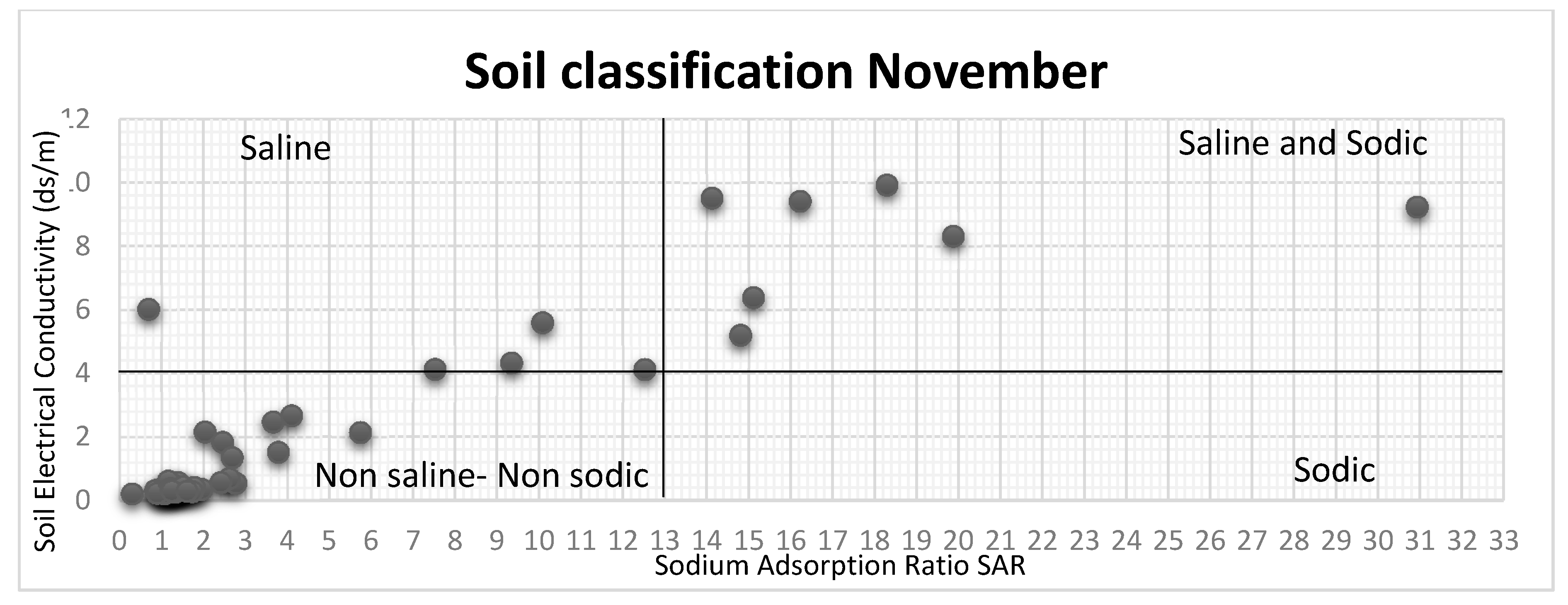
Conventionally, the monitoring process involves the collection of soil and analytical determination of characteristics such as salinity (electrical conductivity, EC), the effects of sodium on soil properties, and the toxicity of specific ions [27]. These have been accompanied by indices such as the Sodium Adsorption Ratio (SAR) [28]. However, knowledge of soil properties is essential for efficient and sustainable soil and water management of agricultural land, especially in desert oases [29], and mapping them can supply an overview of the problems and how farmers can act to solve them.
Geostatistics is considered an effective tool for the detection, monitoring and mapping of salt-affected areas and their spatio-temporal variations [30,31,32]. In many cases, the Kriging method proved to be the best estimator, i.e., ordinary Kriging (OK), while inverse distance weighting (IDW) or splines were considered appropriate methods in other cases [33,34,35,36,37]. The interpolation based on inverse distance weight (IDW) is an accurate method for mapping saline soils, according to Farajnia and Yarahmadi (2017) [38]. In addition, many studies using soil-landscape analysis have shown that it can be a very good indicator of the distribution of soil properties in space [39].
Few studies have focused on the interaction between the main factors that cause the spatial distribution of soil salinity, and there is a lack of knowledge about how these factors interact with each other [40]. It is therefore necessary to detect, monitor and map the salinity of soils in space and time in order to avoid further soil degradation and to ensure the sustainable development of agriculture [41,42].
However, little work has been done on the spatial variability of soil properties in the province of Ghardaïa (South Algeria); therefore, we have carried out this study to (1) evaluate quality of soil properties and monitor the dynamics of soil salinity, (2) compare two spatial interpolation techniques (IDW, OK) in order to highlight the spatial distribution of soil salinity, and (3) detect the main problems concerning salinity in order to favor the maintenance and sustainability of the oasis agrosystem.

2. Materials and Methods

2.1. Study Area

The study area is a date palm grove known as “El Hadjra el Bidha” (32°24′5.80″–32°24′31.79″ North Latitude; 4°14′37.40″–4°14′41.70″ East Longitude) and located in Zelfana, a municipality of the province of Ghardaïa, in Central Algeria. It is 67 km East of the wilaya of Ghardaia. (Figure 1). It has an extension of 42 ha, which is divided into plots with surfaces of about 1 ha. These were planted with date palms (Phoenix dactylifera L.) in 1975 (according to farmers’ accounts) with a spacing of 9 m between plants. This site was an ancient oasis, which is divided into individual plots of almost the same size. The plant density is about 160 palms/ha, and the average height is between 8–10 m.
The region is part of the Great Desert, which is characterized by short and rigorous winters, while the summers are long and hot. The average annual temperature exceeds 25 °C. July is the hottest month (41.50 °C), while January is the coldest (6.20 °C). Rain is rare and irregular, with average annual rainfall ranging from 100 to 200 mm/year, with evaporation of 2000 mm per year [43].
The study area is characterized by an almost equal topography, with a difference of altitude not exceeding 1.5 m between the highest and the lowest points of the palm grove (highest point in the NW to the lowest point in the SE); the slope is under 0.5%. The soils in the region are mainly classified as Psamment in the Soil Taxonomy [44]; these are soils with a sandy texture, which consist of unconsolidated sand deposits or Arenosols, considering the World Reference Base for Soil Resources (WRB) [45]. After intensive cultivation for long periods, the agricultural soils of these oases can be considered Anthrosols (WRB).
The slope of the palm grove goes from the northwest (NW) to the southeast (SE) of the study area, determining the water flow. There, a non-permanent natural watercourse where water intermittently runs only a few days a year is located. This system acts as natural drainage for the area and the oasis.
The soil is irrigated with water from the Continental Interlayer. Each plot is fed by a tertiary network of open concrete canals (Seguias) that carry the water to the entrances of the plots. Irrigation is organized in rotation with one water turn per week, and farmers have water determined according to the number of palm groves. The recommended standard for a palm grove is more than 70 L/s·ha, and the daily cycle does not exceed 7 days [46]. In our case, the amount of irrigation does not exceed 50 L/s·ha, and the daily cycle is in some cases 8 days. In summer, the amount decreases up to 50%. This quantity does not cover the needs of the plants. In addition, ditches and canals are in poor condition to provide good drainage. The drainage canals are about 1 m deep, located around the orchards, forming the drainage system. However, the abandonment of the ditches leads to stagnation of drainage water due to poor management of the system.
In order to improve the organic fertility of the soil, farmers add around 20 to 30 kg of sheep manure and cover it with sand at the bottom of each date palm to prepare for cultivation.

2.2. Soil Sampling and Analysis

To explore the spatial distribution of soil salinity, soil samples were taken according to systematic planning covering the entire study area and ensuring at least one sample per plot (Figure 1). Samples were taken beside the palm tree, approximately 1.5 m from the stipe. 45 soil-sampling points were taken in 2018 in two periods: May and November. These two months coincide with a period of major agricultural work (beginning of the fruiting season and end of fruit maturation) [47]. At each point, we took 0–30 cm depth samples (topsoil).
The samples obtained were transferred to the laboratory and air dried, crushed and sieved at 2 mm. In the fine earth, electrical conductivity was determined in water extraction (EC; ratio 1:2.5 w/v) following the procedure described by the United States Salinity Laboratory (USDA) [28]. This method consists of mixing the sample with a lot of water to obtain a very strongly diluted solution. It allows for maximum extraction of salts as opposed to saturated paste extracts, the soil/water ratio remaining constant whatever the texture of the sample [48]. Soluble cations (Na+. Ca2+ and Mg2+) were analyzed using standard USDA procedures [49].
The SAR was calculated by computing Na+, Ca2+ and Mg2+ concentrations (in meq/L) from the saturation extract (Equation (1)).
S A R = Na + 1 2 ( Ca 2 + + Mg 2 + )

2.3. Characteristics of Irrigation Water

The sustainability of agricultural yield in oases depends on the quality and quantity of irrigation water. In our study area, soils are irrigated with water from the Continental Interlayer. Table 1 shows the mean physico-chemical characteristics of the water used for irrigation and drainage water, taken in June (Figure 2). Knowing that all the soils were irrigated with the same water, the salinity may be influenced by other factors like farm management and environmental conditions.

2.4. Statistical Analysis

The data were subjected to a standard analysis to obtain descriptive statistics, specifically the mean, minimum and maximum, median, variance, standard deviation (SD), coefficient of variation (CV), kurtosis and skewness of each parameter. To identify the normal distribution of the data, skewness is the most common statistical parameter used with values ranging from −1 to +1. For this preliminary analysis, the normality of the data was assessed before using geostatistics to obtain prediction maps. The normality of each dataset was additionally verified by the (QQ plot) test to ensure normal distribution.

2.5. Predictive Mapping

The IDW and OK geostatistical techniques were used to determine the spatial variability of soil salinity in both periods (spring and autumn). Moreover, after that, we compare the two methods by using ME and RMSE.

2.5.1. The IDW Interpolation

The Inverse Distance Weighting (IDW) interpolation is a spatial prediction technique [50] commonly used in Geosciences. This tool attributes each entry point to a local influence that decreases with distance and calculates the values of prediction for an unknown interpolated point by weighting the medium of known data point values. This method can be used if enough sample points have a distribution that occupies the area on a local scale. It weights the points nearest to the prediction point to those more distant. IDW is an exact and convex interpolation method that adapts only to the continuous model of spatial variation.
A general form of predicting an interpolated value Z at a given point x based on samples Zi = Z(xi) for i = 1, 2, …, N using IDW is an interpolating function:
Z ( x ) = i = 1 n ω i ( x ) z i j = 1 n ω j ( x ) , ω i ( x ) =   1 d ( x , x i ) α
As defined by Shepard [50], the equation presented above designates a simple IDW weighting function, where x stands for the predicated location of an unknown interpolated point, xi is the known data point, d is the distance from xi to x, n refers to number of points used in interpolation, and p resembles an arbitrary real positive number known as the distance-decay or the power parameter (normally α = 2 in the standard IDW). Note that in the standard IDW, parameter α is a specified constant value defined by the user for all unknown interpolated points [51]. The selected interpolation technique is commonly used for this type of study and is the most common scatter-point interpolation method. It is based on the fundamental assumption that the interpolation surface should be influenced most by near points and least by far points. The interpolation surface is a weighted average of scattering points, and the weight assigned to each scattering point decreases as the distance between the interpolation point and the scattering point increases. In fact, values at unknown points are calculated as a weighted average of the values available at known points [52,53].

2.5.2. The Ordinary Kriging Interpolation

Kriging is a group of geostatistical methods for interpolating the values of different regional variables at an unobserved location from observations of its value at nearby locations, consisting of ordinary Kriging, universal Kriging, indicator Kriging, co-Kriging, and others [54,55,56].
Ordinary Kriging (OK) is a commonly used method [57], and it was applied in this study. The OK method plays a special role because it is compatible with a stationary model, involves only the variogram, and it is in fact the form of Kriging that is most often used [58,59].
This method estimates the values of a target variable in unmeasured locations, where Z*(x0) is at an unsampled location, using measured values Z(xi) (i = 1, 2, …, N), [60,61] as follows:
z * ( x 0 ) = i = 1 n λ i   z ( x i )
λi returns the weight attributed to the i observation. According to [62], weights are assigned to each sample so that the variance of the estimate is minimized and estimates are unbiased.
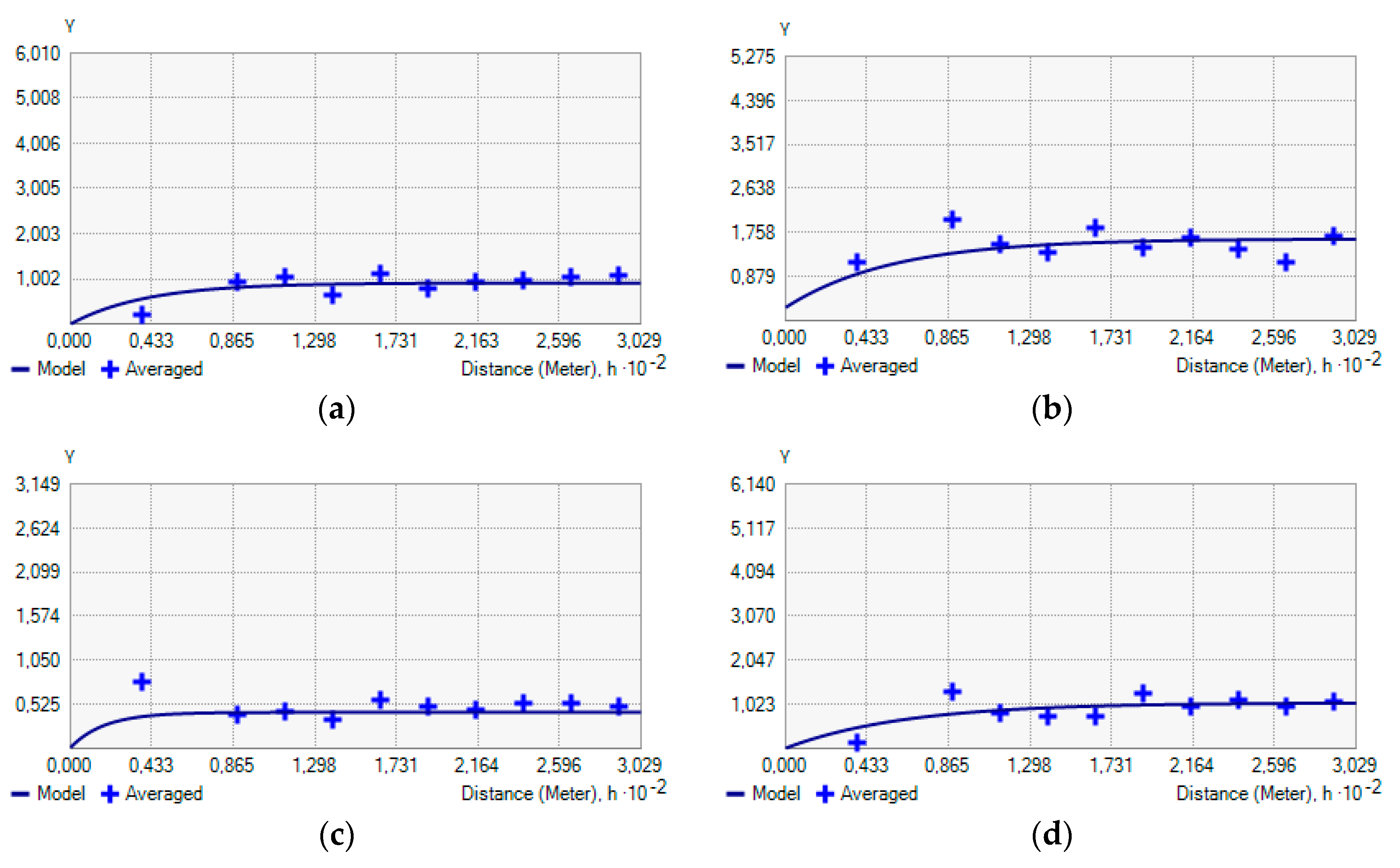
Semivariograms are considered a basic tool for assessing the spatial distribution of soil properties. Based on the theory of regionalized variables and intrinsic assumptions [63], a semivariogram is expressed as follows:
γ ( h ) = 1 2 N ( h ) Σ i = 1 N ( h ) [ Z ( x i ) Z ( x i + h ) ] 2
where γ ( h ) is the semivariance, h is the lag distance, Z is the parameter of the soil property, N ( h ) is the number of pairs of locations separated by a lag distance h , Z ( x i ) , and Z ( x i + h ) are values of Z at positions x i and x i + h [64].

2.6. Comparison of Methods

For better selection of the method used to determine the spatial variability of soil salinity, both interpolation methods have been evaluated to verify the compatibility of the relative performance of IDW and OK [65].
In order to evaluate the accuracy of the determined model, two statistical indices, such as the Mean Error (ME) and the Root Mean Square Error (RMSE), were calculated using the following equations:
-
Mean error:
M E = 1 N i = 1 N ( Z * ( x i ) Z ( x i ) )
-
Root mean square error:
R M S E = Σ i = 1 N (   Z * ( x i ) Z ( x i ) ) 2 N
where Z(xi) is the observed value at location i, Z*(xi) is the predicted value at location i, and n is the sample size. Squaring the difference at any point gives an indication of the magnitude of differences, in such a way that a value of RMSE close to zero illustrates the accuracy of the prediction of the model. It is assumed that if the variogram model is correct, ME should be almost zero [66,67,68].
According to [68,69,70], the indicator of spatial dependence can be classified according to the nugget/sill ratio. The variable considers a strong spatial, a moderate spatial and a weak spatial dependence if the ratio is ≤25%, 25–75% and ≥75%, respectively.
The choice of an appropriate method depends on the particularities of the data and the type of spatial model desired. The accuracy of prediction of ordinary Kriging (OK) and inverse distance weighted (IDW) was evaluated by using the electrical conductivity and SAR data.
All data processing and analysis was carried out using ArcGis 10.2 © software and statistical processing with Microsoft Excel ©.

3. Results and Discussion

3.1. Soil Characteristics

3.1.1. Soil Salinity

As a common rule, high concentrations of salts in the irrigation water and the nature of the hyper-arid climate, combined with many other factors, significantly influence soil quality, causing an increased presence of salts in the root zone and leading to a reduction in crop growth and agricultural yields [71,72]. However, the quality of the irrigation water in our agrosystem is admissible, and the salinity maybe associated with salts remaining in the soil after a long period of cultivation. This may be a consequence of climatic conditions and the accumulation of salts in the topsoil through capillarity during periods where no irrigation is applied (end of autumn and winter).
Statistical analysis of the results (Table 2) reveals that in the first season, the EC value varies between 0.15 dS/m and 7.27 dS/m with a coefficient of variation of 104.84, and the SAR value varies between 1.33 and 16.98 with a coefficient of variation of 77.03. In the second season, the EC value varies from 0.21 dS/m to 9.39 dS/m with a coefficient of variation of 129.94, and the SAR value varies from 0.3 to 30.93 with a coefficient of variation of 131.53. The Coefficient of Variation (CV) can reflect the degree of dispersion of random variables: a CV < 10% generally denotes weak variability, while 10% < CV < 100% denotes moderate variability, and CV > 100% denotes strong variability [73], demonstrating that both conditions exhibit strong variation. In our case, this indicates that both periods exhibit strong variability, except for the SAR in the first period, which exhibits moderate variation. Standard deviation and CV were greater in the second period, indicating more differences associated with the location of sampling points, showing the highest variability in soil salinity.
Based on the classes determined by Durand (1983) [74], who considers five salinity classes (Table 3), more than a third of the soil samples would be considered non-saline soils.
The analysis of this table (Table 3) allows us to observe that the percentages of saline soils in the first and second periods were 41.49% and 34.8%, respectively (yield can be affected), whereas non-saline soils represent 54.17% and 58.68% (productive soil), and 4.34% and 6.52% represented moderately saline soils (soil that can be used for tolerant crops). Moreover, these results show that, even when using the same irrigation water and the same soil sample points, differences in salinity occurred. Even more, important changes were found in the classes with high salinity, maybe due to the movement of salts. However, we can notice that approximately 55–60% of the soils remained in the salinity classes of non-saline soil and slightly saline soil during both periods.
It is important to understand the spatial distribution of salinity in order to check where the salts have been accumulated and, in this sense, make better decisions for managing the system.

3.1.2. Distribution of Soil Salinity Using IDW and OK Interpolation

In this study, interpolation IDW (inverse distance weighting) and OK (ordinary Kriging) were used to estimate the spatial distribution of soil salinity.
IDW is one of the most common techniques for interpolating scattering points and is based on the fundamental assumption that the interpolation area should be influenced most by near points and least by far points. The interpolation area is a weighted average of the scattering points, and the weight assigned to each scattering point decreases as the distance between the interpolation point and the scattering point increases. Values at unknown points are estimated as a weighted average of the values available at known points [52,53]. Summary statistics of IDW interpolation are presented in Table 2. For OK interpolation, the data were verified by a normality test (QQ Plot) to evaluate the distribution of the data, which confirms that the skewness value is greater than 1 (the results do not follow a normal distribution). These data were normalized using the logarithmic decimal method (Table 4).
Subsequently, variograms of the Kriging method were calculated from the normalized data. The best theoretical optimal model used here for EC and SAR in both periods was the Exponential model to estimate the distribution of soil salinity (Table 5).
The spatial dependence “nugget-to-sill” for soil salinity was in the class (<25%), which corresponds to high spatial dependence (Table 5). In addition, the range of the chosen model is 25.243 m (Figure 3).
This information, derived from the semivariograms, highlighted the reality of different spatial dependence for the soil properties collected in the field (Table 5). The proportion of nuggets to the threshold mimics spatial autocorrelation.
The IDW interpolation method (Figure 4) and Ok interpolation (Figure 5) were used to perform a better spatial interpolation method for unsampled points, to obtain the soil salinity distribution pattern in the oasis.
According to the maps of the spatial distribution of EC and SAR using IDW (Figure 4) and OK interpolation (Figure 5), the highest soil salinity (EC) was mainly observed in the southern parts of the study area in the first period, which is related to the direction of irrigation water flow observed during the survey. This could be a result of the stagnation of drainage water due to the presence of a depression nearby that can naturally drain irrigation water. Large quantities of water subjected to evaporation will eventually lead to an increase in salinity, whereas in the second period, the salts migrated to external parts of the study area, which is related to high evaporation due to excessively high temperature and reduced irrigation frequency.
A soil salinity map is needed to assess and monitor salt accumulation. This information can be used as an effective tool to help farmers manage soil salinity problems affecting the agroecosystem. Moreover, the simplicity of this approach, with its satisfactory accuracy, can greatly contribute to the prediction and mapping of soil salinity [67,75]. In this sense, farmers will have information to detect saline soils and improve their management in the next period of cultivation.

3.1.3. Comparison of IDW and OK

The comparison of IDW and OK was performed using ME and RMSE values to define the best method of spatial interpolation suited to the region. Measures for evaluating model performance are summarized in Table 6.
Based on a comparison between the results, the ME of both interpolation methods was satisfactory (values were close to zero) [68,76], but the RMSE value was lower when using IDW. According to these geostatistical results, there was a slight difference in the performance of IDW when predicting salinity, compared with OK. This may explain the good accuracy of the IDW method.
The OK map represented the spatial variability with less detail, demonstrating the importance of this interpolation to variability on long-distance scales, while the IDW map represented the spatial variability with more detail on short-distance scales, supporting fairly dense sampling.
Other studies that have been conducted using this approach, for example [77,78,79], confirm that IDW interpolation is more efficient than OK in predicting distribution, especially of the physico-chemical properties of soil, and this was probably due to the method of sampling and the similar distances of all samples. In contrast, other studies, for example [80,81,82], considered the performance of ordinary Kriging to be the best in comparison with other predicted data and with reference to actual data, concluding that it was also very reliable and more accurate.
We presume that the sampling interval that occupies the entire prediction scale can explain the performance of IDW in interpolating the soil property [65]. Other studies [83,84] provide maps of salinity distribution by using geostatistical methods and considered the co-Kriging method to be the most accurate method for predicting EC and SAR levels. In fact, the sampling method may determine the best geostatistics method.
Understanding and controlling the spatial distribution of soil salinity can provide a database for implementing an agricultural management policy capable of controlling and preventing soil salinization [85]. To explore the spatial variability of soil salinity, we applied a geostatistical method in an agricultural area with an arid climate in order to identify the influencing factors. The analysis of the maps obtained is consistent with the real situation of the terrain, which is characterized by high salinity in areas of stagnant drainage water.
This distribution of soil salinity is explained by the method of irrigation through submersion and the direction of flows used in this agricultural perimeter, coupled with severe climatic conditions, especially in the summer period when temperature and evaporation are excessively high. In addition to this is the poor management of natural resources and modification of soil structure caused by humans.
Our contribution focused, in particular, on oasis farmland in an arid region. The results and methodology could be extended to other regions that experience similar problems in arid and semi-arid areas. Agriculture is critical for many communities, and by understanding and mapping the problems it is possible to achieve sustainability and create opportunities for these communities associated with oasis systems. Therefore, our study will be able to open a path for reflection and research, allowing the implementation of projects dealing with soil salinity on a large scale, as well as a detailed investigation of factors influencing the sustainability of agricultural production in drylands.
It is clear that sustainability is not optional, and we need to know how the system works to improve it [86]. These results enable planners, decision-makers and engineers to undertake and guide agricultural development work, which consists of setting up an adequate drainage network capable of removing excess salt-laden water from the farming area and providing additional irrigation (leaching dose) to maintain drainage channels.
These arid regions are known for the scarcity of water and its high mineralization. In order to avoid aggravating the water crisis and prevent considerable food shortages, the productivity of water use must be increased. Moreover, the treatment and use of agricultural drainage water (ADW) is becoming an obligation for development needs in arid and semi-arid zones [86]. In the future, one option to be considered in these regions is the reuse of agricultural drainage water, which could be treated using recycling techniques [87], for instance, through the establishment of treatment plants and/or the desalination of water by reverse osmosis systems with solar energy supply. In this sense, keeping drainage systems in good conditions is necessary.

3.1.4. Classification of Soil Salinity

After detecting and mapping the salinity, it is important to determine the location of salt-affected soils and the grade of this affection. The soils (sampling points) were classified by comparing the EC, SAR and pH values with the threshold values set by Abegunrin et al. (2013) [88], considering salinity and sodium or alkalinity risks as the EC, SAR and pH values were below 4 dS/m, 13 and 8.5, respectively (Table 7). With the exception of a few samples, most of the soils could be considered non-saline and non-sodic soils (Figure 6).
The Zelfana region has undergone a major change in agriculture compared to oasis agriculture, linked to the almost exclusive production of dates, followed by the production of vegetable crops throughout the year. Irrigation with groundwater can enrich soils with salts or cause their mobility in the soil profile, which is associated with problems of soil management and conservation. This will undoubtedly have negative repercussions on the soil (salinization and sodification leading to degradation of the soil structure) and on agricultural dynamics in Zelfana. The sensitivity of crops to salt stress results in reduced plant growth (reduced leaf length of fronds) and reduced productivity. Each crop has a specific tolerance to saline stress, which can reduce yield by about 50% for several cultivars such as pepper, lettuce and potato for an EC threshold of 5 dS.m−1 [89].
The date palm has a high tolerance for soil salinity [26,90,91,92], but several publications consider that an increase in salinity corresponds to a reduction in yield < 25% [93,94]. According to Ramoliya et al. (2003) [95], this crop can withstand a relatively high salinity of 12.8 ds/m with no visible effect on the fruit, and other varieties of date palms could tolerate up to 9 ds/m of soil salinity [96]. In order to obtain a better quantitative and qualitative yield, it is necessary to consider the nature of the soil and its salinity as well as the crop’s tolerance to salinity, to innovate an adequate strategy to ensure good, efficient and sustainable management capable of maintaining the maximum yield of crops for future generations. One of the best strategies for the rehabilitation of saline soils is the proper selection of crops, not only for economic purposes but also for the control of soil and saline water pollution [97]. Crops could extract salts and act as phytoremediators because of their ability to adapt to local saline environments. Due to the results obtained, it seems that acquisition of the data has given us a clear vision of the current state of soil salinization in this area, which is useful for managers and farmers.
The right choice of market gardening crops according to the nature of the soil requires an adequate selection of crops according to their resistance to saline stress, followed by good use of water resources through the installation of irrigation and drainage networks that will maintain the aquifer level and ensure the discharge of contaminated water below the critical level of salinization in order to guarantee the sustainability of agricultural systems.
In recent years, remote sensing, GIS and modelling have become preferred and inexpensive technological tools for mapping soil salinity due to the large areas covered, which is of utmost importance from both agricultural and environmental perspectives. This opens up great prospects for the use of this technique in the sustainable management of soils.

4. Conclusions

The main objective of this study was to estimate the soil salinity in an oasis by comparing two spatial interpolation techniques based on GIS, in order to highlight a better sustainable management strategy. It is crucial to select an appropriate method for estimating the spatial distribution of soil salinity with minimum error, for good management practices. In this study, IDW and OK were the two methods assessed to study soil salinity in the Zelfana oasis, Ghardaïa. Hence, the IDW method was more accurate than the results obtained by the OK technique for the estimation of salt-affected areas. In our case, the relation between drainage system and soil salinity seems to be a key factor in managing the agrosystem, emphasizing the importance of sustainable water management in oasis systems.
The obtained results showed that the majority of soils belong to a salinity class that can be adequate for date palm tolerance but are not recommended for other crops, especially in the southern part of the study area. Based on the EC, SAR and soil salinity distribution maps, it seems that in this area, soils with high salinity do not support low tolerance market gardening.
Thus, this model (IDW) for monitoring the spatial distribution of soil salinity is a good indicator and can be used by phoeniculturists in the Zelfana oasis and generalized by decision-makers in similar areas, so as to implement effective management programs and the sustainable use of agricultural systems.
To overcome the constraints of field data collection, an extensive data collection, which is regarded as time-consuming and costly, mapped and identified sites where salinity is detected, helping to reduce the number of sample points and determine the actions necessary to maintain the system and aid sustainability in the long-time. However, further research is necessary to investigate the ability to use remote sensing techniques if they can increase the accuracy of soil salinity modeling and mapping for areas dominated mainly by date palm and market gardening in arid environments.

Author Contributions

Conceptualization, A.B.; Methodology, A.B., K.K. and F.B.; Software, A.B., J.N.-P.; Validation, A.B., J.N.-P., F.B.; Formal Analysis, A.B., J.N.-P.; Investigation, A.B., S.B. and F.C.; Resources, A.B., F.C., S.B. and J.N.-P.; Data Curation, A.B., J.N.-P. and F.C.; Writing—Original Draft Preparation, A.B.; Writing—Review & Editing, A.B., J.N.-P.; Supervision, J.N.-P., K.K.; Project Administration, A.B.; Funding Acquisition, A.B., J.N.-P., F.C. All authors have read and agreed to the published version of the manuscript.

Funding

A. Benslama was obtained a scholarship to finalize this work at Miguel Hernandez University in Elche, Spain.

Acknowledgments

This work was funded by the Ministry of Higher Education and Algerian Scientific Research. We would like to express our heartfelt thanks to everyone who has helped us particularly: Benslama Mohamed, director of the laboratory Soils and Sustainable Development, Badji Mokhtar University-Annaba, Algeria. Ignacio Gomez Lucas, the head of the Department of Agrochemistry and Environment. Abdennour M.A, PhD student at the University Mohamed Khider of Biskra, Algeria. The manager of the Horizon Laboratory, Annaba, Mlle. Mohamadi Nadia.

Conflicts of Interest

The authors declare no conflict of interest.

References

  1. Lhissoui, R.; El Harti, A.; Chokmani, K. Mapping soil salinity in irrigated land using optical remote sensing data. Eurasian J. Soil Sci. 2014, 3, 82–88. [Google Scholar] [CrossRef] [Green Version]
  2. Jordán, M.; Navarro-Pedreno, J.; García-Sánchez, E.; Mateu, J.; Juan, P. Spatial dynamics of soil salinity under arid and semi-Arid conditions: Geological and environmental implications. Environ. Geol. 2004, 45, 448–456. [Google Scholar] [CrossRef]
  3. Wu, J.; Vincent, B.; Yang, J.; Bouarfa, S.; Vidal, A. Remote sensing monitoring of changes in soil salinity: A case study in Inner Mongolia, China. Sensors 2008, 8, 7035–7049. [Google Scholar] [CrossRef] [PubMed] [Green Version]
  4. Daoud, Y.; Halitim, A. Irrigation et salinisation au Sahara algérien. Sci. Chang. Planétaires Sécheresse 1994, 5, 151–160. [Google Scholar]
  5. Hachicha, M.; Cheverry, C.; Mhiri, A. The impact of long-term irrigation on changes of ground water level and soil salinity in northern Tunisia. Arid. Soil Res. Rehabil. 2000, 14, 175–182. [Google Scholar] [CrossRef]
  6. Djili, K.; Daoud, Y.; Gaouar, A.; Beldjoudi, Z. La salinisation secondaire des sols au Sahara. Conséquences sur la durabilité de l ‘agriculture dans les nouveaux périmètres de mise en valeur. Sci. Chang. Planétaires Sécheresse 2003, 14, 241–246. [Google Scholar]
  7. Idder, T. Excess water in Ouargla: Present situation and perspectives for improvement. Sci. Chang. Planétaires Sécheresse 2007, 18, 161–167. [Google Scholar]
  8. Abdel-Razek, M.; Gaiser, T.; Diekkrüger, B.; Goldbach, H. Salinity Development during Three Decades in the Oasis of Ktoua, South East Morocco. In ’Tropentag 2010: International Research on Food Security. Natural Resource Management and Rural Development; ETH: Zurich, Switzerland, 2010; pp. 14–16. [Google Scholar]
  9. Douaik, A.; Van Meirvenne, M.; Tóth, T. Stochastic Approaches for Space-Time Modeling and Interpolation of Soil Salinity. In Remote Sensing of Soil Salinization: Impact on Land Management; CRC Press: Boca Raton, FL, USA, 2009; pp. 273–290. [Google Scholar]
  10. Huang, Y.; Wang, Y.; Zhao, Y.; Xu, X.; Zhang, J.; Li, C. Spatiotemporal Distribution of Soil Moisture and Salinity in the Taklimakan Desert Highway Shelterbelt. Water 2015, 7, 4343–4361. [Google Scholar] [CrossRef] [Green Version]
  11. Yang, X.-D.; Ali, A.; Xu, Y.-L.; Jiang, L.-M.; Lv, G.-H. Soil moisture and salinity as main drivers of soil respiration across natural xeromorphic vegetation and agricultural lands in an arid desert region. Catena 2019, 177, 126–133. [Google Scholar] [CrossRef]
  12. Chaieb, G.; Abdelly, C.; Michalet, R. Interactive effects of climate and topography on soil salinity and vegetation zonation in North-African continental saline depressions. J. Veg. Sci. 2018, 30, 312–321. [Google Scholar] [CrossRef]
  13. Wang, J.; Liu, Y.; Wang, S.; Liu, H.; Fu, G. Spatial distribution of soil salinity and potential implications for soil management in the Manas River watershed, China. Soil Use Manag. 2019, 36, 93–163. [Google Scholar] [CrossRef]
  14. Herrero, J.; Castañeda, C. Temporal changes in soil salinity at four saline wetlands in NE Spain. Catena 2015, 133, 145–156. [Google Scholar] [CrossRef] [Green Version]
  15. Yang, F.; An, F.; Ma, H.; Wang, Z.; Zhou, X.; Liu, Z. Variations on Soil Salinity and Sodicity and Its Driving Factors Analysis under Microtopography in Different Hydrological Conditions. Water 2016, 8, 227. [Google Scholar] [CrossRef] [Green Version]
  16. Wang, Z.; Zhou, B.; Pei, L.; Zhang, J.; He, X.; Lin, H. Controlling threshold in soil salinity when planting spring wheat and sequential cropping silage corn in Northern Xinjiang using drip irrigation. Int. J. Agric. Biol. Eng. 2018, 11, 108–114. [Google Scholar] [CrossRef] [Green Version]
  17. Wang, Y.; Xiao, D.; Li, Y.; Li, X. Soil salinity evolution and its relationship with dynamics of groundwater in the oasis of inland river basins: Case study from the Fubei Region of Xinjiang Province, China. Environ. Monit. Assess. 2008, 140, 291–302. [Google Scholar] [CrossRef] [PubMed]
  18. Food and Agricutrual Organization, 2002. The Salt of the Earth: Hazardous for Food Production. Word Food Summit. Five Years Later. 10–13 June 2012. Available online: http://www.fao.org/worldfoodsummit/english/newsroom/focus/focus1.htm (accessed on 5 March 2020).
  19. Pan, X.; Chao, J. Theory of stability, and regulation and control of ecological system in oasis. Glob. Planet. Chang. 2003, 37, 287–295. [Google Scholar] [CrossRef]
  20. The United Nations Educational, Scientific and Cultural Organization. La Lutte contre la Désertification. Ressources en eau Douce et Réhabilitation Des Terres Dégradées Dans Les Zones Arides. In Séminaire International sur la Lutte Contre la Désertification; MAB-UNESCO: N’djamena, Tchad, 2002; p. 135. [Google Scholar]
  21. Halitim, A. Contribution a l’Etude des Sols des Zones Arides (Hautes Plaines Steppiques de l’Algerie): Morphologie, Distribution et Role des Sels dans la Genese et le Comportement des Sols. Ph.D. Thesis, Ecole Nationale Supérieure Agronomique ENSA Alger, Hassen Badi, Algeria, 1985. [Google Scholar]
  22. Berkal, I.; Walter, C.; Michot, D.; Djili, K. Seasonal monitoring of soil salinity by electromagnetic conductivity in irrigated sandy soils from a Saharan oasis. Soil Res. 2014, 52, 769–780. [Google Scholar] [CrossRef]
  23. CISEAU (Centre d’Information Sur l’Eau Agricole et ses Usages). Extent of Salinization and Strategies for Salt-Affected Land Prevention and Rehabilitation: Background Paper. In Electronic Conference on Salinization Organised and Coordinated; IPTRID: Rome, Italy, 2006. [Google Scholar]
  24. Akramkhanov, A.; Vlek, P.L. The assessment of spatial distribution of soil salinity risk using neural network. Environ. Monit. Assess. 2012, 184, 2475–2485. [Google Scholar] [CrossRef]
  25. Food and Agriculture Organization. FAO Statistical Year Book; Food and Agriculture Organization of the United Nations: Rome, Italy, 2012; p. 352. [Google Scholar]
  26. Al-Abdoulhadi, I.; Dinar, H.; Ebert, G.; Bttner, C. Effect of salinity on leaf growth, leaf injury and biomass production in date palm (Phoenix dactylifera L.) cultivars. Indian J. Sci. Technol. 2011, 4, 1542–1546. [Google Scholar] [CrossRef]
  27. Ayers, R.S.; Westcot, D.W. Water Quality for Agriculture; Food and Agriculture Organization of the United Nations: Rome, Italy, 1985; Volume 29. [Google Scholar]
  28. Richards, L. Diagnosis and Improvement of Saline and Alkali Soils. Handbook No. 60; US Department of Agriculture: Washington, DC, USA, 1954. [Google Scholar]
  29. Yang, Y.; Tilman, D.; Lehman, C.; Trost, J. Sustainable intensification of high-Diversity biomass production for optimal biofuel benefits. Nat. Sustain. 2018, 1, 686–692. [Google Scholar] [CrossRef]
  30. Ben-Dor, E.; Patkin, K.; Banin, A.; Karnieli, A. Mapping of several soil properties using DAIS-7915 hyperspectral scanner data—A case study over clayey soils in Israel. Int. J. Remote Sens. 2002, 23, 1043–1062. [Google Scholar] [CrossRef]
  31. Aldabaa, A.A.A.; Weindorf, D.C.; Chakraborty, S.; Sharma, A.; Li, B. Combination of proximal and remote sensing methods for rapid soil salinity quantification. Geoderma 2015, 239, 34–46. [Google Scholar] [CrossRef] [Green Version]
  32. Hasab, H.; Dibs, H.; Dawood, A.; Hadi, W.; Hussain, H.; Al-Ansari, N. Monitoring and Assessment of Salinity and Chemicals in Agricultural Lands by a Remote Sensing Technique and Soil Moisture with Chemical Index Models. Geosciences 2020, 10, 207. [Google Scholar] [CrossRef]
  33. Matheron, G. Kriging or polynomial interpolation procedures. CIMM Trans. 1967, 70, 240–244. [Google Scholar]
  34. Rouhani, S. Comparative study of Ground-Water mapping techniques. Groundwater 1986, 24, 207–216. [Google Scholar] [CrossRef]
  35. Laslett, G.; McBratney, A. Further comparison of spatial methods for predicting soil pH. Soil Sci. Soc. Am. J. 1990, 54, 1553–1558. [Google Scholar] [CrossRef]
  36. Phillips, D.L.; Lee, E.H.; Herstrom, A.A.; Hogsett, W.E.; Tingey, D.T. Use of auxiliary data for spatial interpolation of ozone exposure in southeastern forests. Environ. Off. J. Int. Environ. Soc. 1997, 8, 43–61. [Google Scholar] [CrossRef]
  37. Abed, A.M.; Saffarini, G.A.; Sadaqah, R.M. Spatial distribution of uranium and vanadium in the upper phosphorite member in Eshidiyya basin, southern Jordan. Arab. J. Geosci. 2014, 7, 253–271. [Google Scholar] [CrossRef]
  38. Farajnia, A.; Yarahmadi, J. Soil Salinity and Alkalinity Map Preparation Based on Spatial Analysis of GIS (Case Study: Tabriz Plain). Open J. Geol. 2017, 7, 778–788. [Google Scholar] [CrossRef] [Green Version]
  39. Akramkhanov, A. The Spatial Distribution of Soil Salinity: Detection and Prediction; Cuvillier Verlag: Göttingen, Germany, 2005; Volume 32. [Google Scholar]
  40. Xu, L.; Du, H.; Zhang, X. Spatial Distribution Characteristics of Soil Salinity and Moisture and Its Influence on Agricultural Irrigation in the Ili River Valley, China. Sustainability 2019, 11, 7142. [Google Scholar] [CrossRef] [Green Version]
  41. Li, Y.; Zhao, K.; Ding, Y.; Ren, J. An Empirical Method for Soil Salinity and Moisture Inversion in West of Jilin. In Proceedings of the International Conference on Remote Sensing, Environment and Transportation Engineering (RSETE 2013), Nanjing, China, 26–28 July 2013; Atlantis Press: Paris, France, August 2013; pp. 19–21. [Google Scholar]
  42. Wang, H.; Jia, G. Satellite-Based monitoring of decadal soil salinization and climate effects in a semi-Arid region of China. Adv. Atmos. Sci. 2012, 29, 1089–1099. [Google Scholar] [CrossRef]
  43. ONM (National Office Meterology). Données climatiques de la région de Ghardaïa Algérie; ONM: Alger, Algeria, 2017. (In French) [Google Scholar]
  44. Soil Survey Staff. Soil Taxonomy: A Basic System of Soil Classification for Making and Interpreting Soil Surveys, 2nd ed.; Natural Resources Conservation Service U.S. Department of Agriculture: Washington, DC, USA, 1999.
  45. Wrb, I.W.G. World Reference Base for Soil Resources 2014, Update 2015: International Soil Classification System for Naming Soils and Creating Legends for Soil Maps. In World Soil Resources Reports No. 106; Food and Agriculture Organization of the United Nations: Rome, Italy, 2015; p. 192. [Google Scholar]
  46. Eddine, B.S.; Foued, C. La conduite du palmier dattier dans les palmeraies des zibans (algérie) quelques éléments d’analyse. Eur. J. Sci. Res. 2010, 42, 644–660. [Google Scholar]
  47. Toutain, G. Le palmier dattier: Culture et production. Al Awamia 1967, 25, 83–151. [Google Scholar]
  48. Diba, M. Analyse Comparée de Deux Méthodes d’Evaluation de la Répartition Spatiale de la Salinité des Sols: La Pâte Saturée (Méthode de Réference), la Conductivimétrie Eléctromagnétique. Ph.D. Thesis, Mémoire d’Ingénieur, Dakar, Senegal, 1995. [Google Scholar]
  49. Oil Survey Division Staff. Soil Survey Manual. USDA Handbook No. 18; U.S. Government Printing Office: Washington, DC, USA, 1993.
  50. Shepard, D. A Two-Dimensional Interpolation Function for Irregularly-Spaced Data. In Proceedings of the 1968 23rd ACM National Conference, New York, NY, USA, 27–29 August 1968; pp. 517–524. [Google Scholar]
  51. Mei, G.; Xu, L.; Xu, N. Accelerating adaptive IDW interpolation algorithm on a single GPU. arXiv 2015, arXiv:1511.02186. [Google Scholar]
  52. Yasrebi, J.; Saffari, M.; Fathi, H.; Karimian, N.; Moazallahi, M.; Gazni, R. Evaluation and comparison of Ordinary Kriging and Inverse Distance Weighting methods for prediction of spatial variability of some soil chemical parameters. Res. J. Biol. Sci. 2009, 4, 93–102. [Google Scholar]
  53. Zimmerman, D.; Pavlik, C.; Ruggles, A.; Armstrong, M.P. An experimental comparison of ordinary and universal kriging and inverse distance weighting. Math. Geol. 1999, 31, 375–390. [Google Scholar] [CrossRef]
  54. Bayraktar, H.; Turalioglu, F.S. A Kriging-Based approach for locating a sampling site—In the assessment of air quality. Stoch. Environ. Res. Risk Assess. 2005, 19, 301–305. [Google Scholar] [CrossRef]
  55. Emery, X. Simple and ordinary multigaussian kriging for estimating recoverable reserves. Math. Geol. 2005, 37, 295–319. [Google Scholar] [CrossRef]
  56. Hormozi, H.; Hormozi, E.; Nohooji, H.R. The classification of the applicable machine learning methods in robot manipulators. Int. J. Mach. Learn. Comput. 2012, 2, 560. [Google Scholar] [CrossRef]
  57. Lefohn, A.S.; Knudsen, H.P.; Shadwick, D.S. Using Ordinary Kriging to Estimate the April–September 24-Hour W126 and N100 Ozone Exposure Metrics for 2010 for the United States. 2011. Available online: https://webcam.srs.fs.fed.us/ozone/spatial/2010/contractor_2010.pdf (accessed on 27 July 2020).
  58. Chiles, J.; Delfiner, A. Geostatistics: Modelling Spatial Uncertainty; Wiley interscience: New York, NY, USA, 1999. [Google Scholar]
  59. Afzal, P.; Alghalandis, Y.F.; Khakzad, A.; Moarefvand, P.; Omran, N.R. Delineation of mineralization zones in porphyry Cu deposits by fractal Concentration–Volume modeling. J. Geochem. Explor. 2011, 108, 220–232. [Google Scholar] [CrossRef]
  60. Kavianpoor, H.; Ouri, A.E.; Jeloudar, Z.J.; Kavian, A. Spatial variability of some chemical and physical soil properties in Nesho Mountainous Rangelands. Am. J. Environ. Eng. 2012, 2, 34–44. [Google Scholar] [CrossRef]
  61. Wackernagel, H. Cokriging versus kriging in regionalized multivariate data analysis. Geoderma 1994, 62, 83–92. [Google Scholar] [CrossRef]
  62. Webster, R.; Oliver, M.A. Geostatistics for Environmental Scientists; John Wiley & Sons: Chichester, UK, 2007. [Google Scholar]
  63. Nielsen, D.R.; Wendroth, O. Spatial and Temporal Statistics: Sampling Field Soils and Their Vegetation; Catena Verlag: Reiskirchen, Germany, 2003. [Google Scholar]
  64. Wang, Y.; Shao, M. Spatial variability of soil physical properties in a region of the Loess Plateau of PR China subject to wind and water erosion. Land Degrad. Dev. 2013, 24, 296–304. [Google Scholar] [CrossRef]
  65. Mueller, T.G.; Pusuluri, N.B.; Mathias, K.K.; Cornelius, P.L.; Barnhisel, R.I.; Shearer, S.A. Map Quality for Ordinary Kriging and Inverse Distance Weighted Interpolation. Soil Sci. Soc. Am. J. 2004, 68, 2042–2047. [Google Scholar] [CrossRef]
  66. Wackernagel, H. Cokriging. In Multivariate Geostatistics; Springer: New York, NY, USA, 1995; pp. 144–151. [Google Scholar]
  67. Fourati, H.T.; Bouaziz, M.; Benzina, M.; Bouaziz, S. Detection of terrain indices related to soil salinity and mapping Salt-Affected soils using remote sensing and geostatistical techniques. Environ. Monit. Assess. 2017, 189, 177. [Google Scholar] [CrossRef] [PubMed]
  68. Arslan, H. Spatial and temporal mapping of groundwater salinity using ordinary kriging and indicator kriging: The case of Bafra Plain, Turkey. Agric. Water Manag. 2012, 113, 57–63. [Google Scholar] [CrossRef]
  69. Cambardella, C.A.; Moorman, T.B.; Novak, J.M.; Parkin, T.B.; Karlen, D.L.; Turco, R.F.; Konopka, A.E. Field-Scale Variability of Soil Properties in Central Iowa Soils. Soil Sci. Soc. Am. J. 1994, 58, 1501–1511. [Google Scholar] [CrossRef]
  70. Bradaï, A.; Douaoui, A.; Bettahar, N.; Yahiaoui, I. Improving the prediction accuracy of groundwater salinity mapping using indicator kriging method. J. Irrig. Drain. Eng. 2016, 142, 04016023. [Google Scholar] [CrossRef]
  71. Ghassemi, F.; Jakeman, A.J.; Nix, H.A. Salinisation of Land and Water Resources: Human Causes, Extent, Management and Case Studies; CABI: Wallingford, Oxon, UK, 1997; p. 526. Available online: https://www.cabdirect.org/cabdirect/abstract/19976767459 (accessed on 27 July 2020).
  72. Essien, O.; Ubit, F. Investigation of Ikpa river water quality with consideration for domestic and agricultural uses. Wudpecker J. Agric. Res. 2013, 2, 315–323. [Google Scholar]
  73. Nielsen, D.; Wierenga, P.; Biggar, J. Spatial soil variability and mass transfers from agricultural soils. Chem. Mobil. React. Soil Syst. 1983, 11, 65–78. [Google Scholar]
  74. Durand, J.H. Les Sols Irrigables; Etude Pedologique; Presses Universitaires de France: Paris, France, 1983. [Google Scholar]
  75. Mulla, D.; McBratney, A. Soil Spatial Variability. In Handbook of Soil Science; Sumner, M.E., Ed.; CRC Press: Boca Raton, FL, USA, 2000; pp. A-321–A-352. [Google Scholar]
  76. Sun, Y.; Kang, S.; Li, F.; Zhang, L. Comparison of interpolation methods for depth to groundwater and its temporal and spatial variations in the Minqin oasis of northwest China. Environ. Model. Softw. 2009, 24, 1163–1170. [Google Scholar] [CrossRef]
  77. Corwin, D.; Lesch, S.; Oster, J.; Kaffka, S. Monitoring management-Induced spatio–Temporal changes in soil quality through soil sampling directed by apparent electrical conductivity. Geoderma 2006, 131, 369–387. [Google Scholar] [CrossRef]
  78. Robinson, T.; Metternicht, G. Testing the performance of spatial interpolation techniques for mapping soil properties. Comput. Electron. Agric. 2006, 50, 97–108. [Google Scholar] [CrossRef]
  79. Wang, H.; Ren, S.; Hao, Z.; Meng, L.; Wei, W.; Jing, C. Quantitative Evaluation and Uncertainty Assessment on Geostatistical Simulation of Soil Salinity Using Electromagnetic Induction Technique. J. Environ. Prot. 2016, 7, 844–854. [Google Scholar] [CrossRef] [Green Version]
  80. Keshavarzi, A.; Sarmadian, F. Mapping of spatial distribution of soil salinity and alkalinity in a Semi-Arid region. Ann. Wars. Univ. Life Sci. SGGW. Land Reclam. 2012, 44, 3–14. [Google Scholar] [CrossRef]
  81. Reza, S.; Sarkar, D.; Baruah, U.; Das, T. Evaluation and comparison of ordinary kriging and inverse distance weighting methods for prediction of spatial variability of some chemical parameters of Dhalai district, Tripura. Agropedology 2010, 20, 38–48. [Google Scholar]
  82. Tripathi, R.; Nayak, A.; Shahid, M.; Raja, R.; Panda, B.; Mohanty, S.; Kumar, A.; Lal, B.; Gautam, P.; Sahoo, R. Characterizing spatial variability of soil properties in salt affected coastal India using geostatistics and kriging. Arab. J. Geosci. 2015, 8, 10693–10703. [Google Scholar] [CrossRef]
  83. Hosseini, E.; Gallichand, J.; Marcotte, D. Theoretical and experimental performance of spatial interpolation methods for soil salinity analysis. Trans. ASAE 1994, 37, 1799–1807. [Google Scholar] [CrossRef]
  84. Shi, P.; Rui, X. Comparison and improvement of spatial rainfall interpolation methods. J. Hehai Univ. (Nat. Sci.) 2005, 33, 361–365. (In Chinese) [Google Scholar]
  85. Wang, J.; Ding, J.; Yu, D.; Ma, X.; Zhang, Z.; Ge, X.; Teng, D.; Li, X.; Liang, J.; Lizaga, I. Capability of Sentinel-2 MSI data for monitoring and mapping of soil salinity in dry and wet seasons in the Ebinur Lake region, Xinjiang, China. Geoderma 2019, 353, 172–187. [Google Scholar] [CrossRef]
  86. Talaat, H.A.; Ahmed, S.R. Treatment of aricultural drainage water: Technological schemes and financial indicators. Desalination 2007, 204, 102–112. [Google Scholar] [CrossRef]
  87. Tanji, K.K.; Kielen, N.C. Agricultural Drainage Water Management in Arid and Semi-Arid Areas; FAO: Rome, Italy, 2002. [Google Scholar]
  88. Abegunrin, T.; Awe, G.; Idowu, D.; Onigbogi, O.; Onofua, O. Effect of kitchen wastewater irrigation on soil properties and growth of cucumber (Cucumis sativus). J. Soil Sci. Environ. Manag. 2013, 4, 39–145. [Google Scholar] [CrossRef]
  89. Kotuby-Amacher, J.; Koenig, R.; Kitchen, B. Salinity and Plant Tolerance; Electronic Publication AG-SO-03; Utah State University Extension: Logan, UT, USA, 2000; Available online: https://digitalcommons.usu.edu/extension_histall/43 (accessed on 27 July 2020).
  90. Bouhoun, M.D. Contribution à l’Etude de l’Impact de la Nappe Phréatique et des Accumulations Gypso-Salines sur l’Enracinement et la Nutrition du Palmier Dattier dans la Cuvette de Ouargla (Sud Est Algérien). Ph.D. Thesis, Université Badji Mokhtar Annaba, El Bouni, Algeria, 2010. [Google Scholar]
  91. Alhammadi, M.; Glenn, E. Detecting date palm trees health and vegetation greenness change on the eastern coast of the United Arab Emirates using SAVI. Int. J. Remote Sens. 2008, 29, 1745–1765. [Google Scholar] [CrossRef]
  92. Hussain, N.; AI-Rawahy, S.; Rabee, J.; Al-Amri, M.; Causes, O. Genesis and Extent of Soil Salinity in the Sultanate of Oman Pak. J. Agric. Sci 2006, 43, 1–2. [Google Scholar]
  93. Allbed, A.; Kumar, L. Soil salinity mapping and monitoring in arid and Semi-Arid regions using remote sensing technology: A review. Adv. Remote Sens. 2013, 2, 13. [Google Scholar] [CrossRef] [Green Version]
  94. Abrol, I.; Yadav, J.S.P.; Massoud, F. Salt-Affected Soils and Their Management; Food & Agriculture Org.: Rome, Italy, 1988. [Google Scholar]
  95. Ramoliya, P.; Pandey, A. Soil salinity and water status affect growth of Phoenix dactylifera seedlings. N. Z. J. Crop. Hortic. Sci. 2003, 31, 345–353. [Google Scholar] [CrossRef] [Green Version]
  96. Alrasbi, S.A.R.; Hussain, N.; Schmeisky, H. Evaluation of the Growth of Date Palm Seedlings Irrigated with Saline Water in the Sultanate of Oman. ISHS Acta Hortic. 2010, 882, 233–246. [Google Scholar] [CrossRef]
  97. Niñerola, V.B.; Navarro-Pedreño, J.; Lucas, I.G.; Pastor, I.M.; Vidal, M.M.J. Geostatistical assessment of soil salinity and cropping systems used as soil phytoremediation strategy. J. Geochem. Explor. 2017, 174, 53–58. [Google Scholar] [CrossRef]
Figure 1. Location of the study area of Zelfana (Algeria) and the position of soil samples in the orchards.
Sustainability 12 06117 g001
Figure 2. Distribution of irrigation water and drainage in the study area. Sample points of irrigated and drained water are indicated.
Sustainability 12 06117 g002
Figure 3. The experimental Exponential variogram of the: (a) electrical conductivity of soil in May, (b) electrical conductivity of soil in November, (c) Sodium Adsorption Ratio in May, and (d) Sodium Adsorption Ratio in November.
Sustainability 12 06117 g003
Figure 4. Distribution maps of soil EC (a,b) and Sodium Adsorption Ratio (SAR, c,d) by using inverse distance weighting (IDW) in May (M) and November (N) respectively.
Sustainability 12 06117 g004
Figure 5. Distribution maps of soil salinity (a,b) and SAR (c,d) by ordinary Kriging (OK) in May (M) and November (N) respectively.
Sustainability 12 06117 g005
Figure 6. Classification of soils (sampling points) according to Abegunrin et al. (2013) [88].
Sustainability 12 06117 g006aSustainability 12 06117 g006b
Table 1. Mean value of the physico-chemical characteristics of irrigation/drainage water.
pHEC (dS/m)Salinity (mg/L)Na+ (meq/L)Ca2+ (meq/L)Mg2+ (meq/L)K+ (meq/L)Cl (meq/L)NO3 (meq/L)SO42− (meq/L)
IRRIGATION7.51.99116.129.115.630.3910.450.392.48
DRAINAGE7.65.9341017.434.6516.570.8725.350.883.10
Table 2. Mean values and statistics of soil properties in both sampling periods: May and November.
ParameterEC (dS/m)SAR
MAYMean1.875.65
Max7.2716.98
Min0.151.33
St.dev1.964.35
CV(%)104.8477.03
Skewness1.241.34
Kurtosis0.540.83
Variance3.8418.91
Median0.83.76
NOVEMBERMean2.325.05
Max9.9330.93
Min0.210.3
St.dev3.016.64
CV (%)129.94131.53
Skewness1.462.07
Kurtosis0.894.37
Variance9.0744.07
Median0.561.76
Table 3. Classification of soil by based on the electrical conductivity (EC) classification supplied by Duran (1983) [74] and the percentage of them associated withs salinity classes (May and November).
CE dS/m Salinity Classes% Soils (May)% Soils (Nov)
≤0.6Non-saline soil41.1354.34
0.6 < EC ≤ 1Slightly saline soil13.044.34
1 < EC ≤ 2Moderately saline soil4.346.52
2 < EC ≤ 4Very saline soil23.918.7
>4Extremely saline soil17.5826.1
Table 4. Descriptive statistics after logarithmic transformation.
MayNovember
MinMaxMeanMedianSt.devSkewnessMinMaxMeanMedianSt.devSkewness
EC (dS/m)−1.881.980.07−0.211.120.16−1.582.290.02−0.561.310.49
SAR0.282.831.491.330.70.3−1.193.430.990.571.090.62
Table 5. Parameters of the optimized variogram model.
MAYNovember
Best-Fit ModelNugget (C0)Sill (C0+C)Range (m)Ratio %Best-Fit ModelNugget (C0)Sill (C0+C)Range (m)Ratio %
ECExponential0.0010.909120.46170.11Exponential0.2651.368170.00119.37
SARExponential0.0130.41854.03443.11Exponential0.01051.053190.0040.99
Table 6. ME and RMSE obtained for IDW and OK interpolations.
ECSAR
MAYNOVEMBERMAYNOVEMBER
MERMSEMERMSEMERMSEMERMSE
IDW−0.0031.9420.0443.4070.084.69−0.037.16
OK−0.0161.950−0.1323.465−0.1044.501−0.4957.45
ME = Mean error, RMSE = root mean square error.
Table 7. Classification of soil based on EC, pH, SAR by Abegunrin et al. (2013) [88].
Soil ClassificationECpHSAR
Normal<4<8.5<13
Saline>4<8.5<13
Sodic<4>8.5>13
Saline and Sodic>4>8.5>13

