Gender Gaps in the Use of Urban Space in Seoul: Analyzing Spatial Patterns of Temporary Populations Using Mobile Phone Data

Department of Urban Planning and Landscape Architecture, Gachon University, 1342 Seongnamdaero, Sujeong-gu, Seongnam 13120, Korea
*
Authors to whom correspondence should be addressed.
Sustainability 2020, 12(16), 6481; https://0-doi-org.brum.beds.ac.uk/10.3390/su12166481
Submission received: 22 June 2020
/
Revised: 29 July 2020
/
Accepted: 10 August 2020
/
Published: 11 August 2020
(This article belongs to the Collection Sustainable Smart Cities and Villages)
Abstract
:This study aims to examine the gender gaps in the use of urban space in Seoul, Korea, to provide empirical evidence for urban planning for gender equality. We analyzed daily temporary populations that were estimated using mobile phone data. We used the total, women’s, and men’s temporary populations as well as the subtraction of the temporary population of men from that of women (SMW) as dependent variables. We first conducted a visual analysis on temporary population density using kernel density estimation and then conducted a further analysis using spatial autocorrelation indicators and spatial regression models. The results demonstrate that: (1) Temporary population patterns for women and men showed similarities in that both were larger in business areas than in residential areas, which means that a large number of women were engaged in economic activities like men; (2) the pattern for SMW showed the opposite, that is, women were more active in residential areas and areas where neighborhood retail shops, cultural facilities, parks, and department stores were easily accessible; and (3) both women’s temporary population and SMW had spatial autocorrelation and thus showed clustering patterns that can be helpful in urban planning for gender equality in Korea.
1. Introduction
This study examined gender gaps in the use of urban space in Seoul, Korea, to provide empirical evidence for urban planning for gender equality by studying the temporary population estimated using mobile phone data. “Temporary population” refers to a population that exists in a certain area during a specific period of time. This study specifically examined daily temporary population.
Gender equality is an ongoing issue that has been debated for over a hundred years, and its importance is still increasing through global democratization and cultural change [1]. Establishing the right relationship between men and women is essential for human sustainability [2]. The International Labor Organization (ILO) declared gender equality “as a matter of human rights, social justice, and sustainable development” [3] (p. 92). Gender issues continue to be discussed in most fields, including labor, education, health, and politics. For example, the Global Gender Gap Report, which was first published by the World Economic Forum, evaluates countries in four categories: Economic participation and opportunity, educational attachment, health and survival, and political empowerment [4].
In the field of urban theory and planning, scholars began to criticize urban planners in the 1970s for creating an urban environment that prioritizes men’s needs [5,6,7]. Since then, they have sought alternative approaches to creating urban spaces that meet men and women’s needs equally [8,9,10,11]. However, despite academic efforts devoted to gender equality, the practical application of gender perspectives remains limited [12], which may be partially due to the lack of objective data evidencing the disparities between women’s and men’s use of urban space [13]. Even if it is self-evident that there is gender inequality in terms of access to and use of urban space, it is important to understand how inequality occurs to provide practical alternatives for improvement. The ILO states that “gender equality...does not mean that women and men have to become the same, but that their rights, responsibilities and opportunities will not depend on whether they were born male or female” [3] (pp. 91–92); this means that gender equality is not nominal equality that treats men and women the same, but rather true equality that reflects the needs of each on the premise that there are physical and social differences between them. To incorporate true gender equality in urban planning, information on the differences between men’s and women’s uses of urban space is first necessary, and the more detailed the information, the more precise planning can be achieved. In other words, data on the scale of daily life are needed to ensure changes at a level that people can perceive in everyday life.
Despite the need for objective data on gender differences in the use of urban space, there have not been many empirical studies on how each gender uses urban space in everyday life. One of the major reasons for the scarcity of research has been the difficulty of collecting micro and dynamic data that capture people’s spatial behaviors in daily urban environments. Although some researchers have used census data to investigate gender differences in spatial patterns in cities [14,15,16], census data, which are collected every 5 or 10 years with a large census output area, provide little information to demonstrate dynamic daily patterns at a micro-level.
To understand spatial patterns of daily life, dynamic information such as temporary population, rather than static data such as residential populations found in census data, is required. Temporary populations can be estimated indirectly from symptomatic indicators such as electricity use, or directly by counting or surveying the number of people present at specific locations and times [17]. However, indirect estimates have limitations in terms of accuracy, and direct estimates are too expensive to carry out on a large scale for a long time. Only recently, large-scale collection of such data has become possible in many countries with the development of information and communication technologies (ICT), including mobile phones and Wi-Fi [17,18]; as a result, studies on temporary populations using ICT data have begun to emerge [18].
Among the available ICT data, this study used mobile phone data to estimate temporary populations by gender. Specifically, the mobile phone data, which provide real-time location information of individuals, enable the analysis of detailed patterns in the use of urban space. In addition, temporary populations can be estimated for various time ranges depending on the purpose of research, such as the population in an hour, a day, a week, or a year [19]. We defined temporary population for this study as the one-day population because this study aimed to analyze gender differences in daily use of urban space.
Using daily temporary populations, this study sought to analyze how gender-specific differences occur in the use of space, to develop and verify statistical models to explain spatial patterns, and to deduce the causes of such differences. Specifically, kernel density was first used to visually analyze the density of temporary populations. The spatial autocorrelation of temporary populations was then analyzed using Moran’s I and local indicators of spatial association (LISA). Subsequently, spatial regression models, such as a spatial lag model (SLM) and a spatial error model (SEM), were used to analyze the influencing factors of temporary populations.
To derive implications for gender-sensitive planning, data on gender differences are necessary instead of simply data on women. In the same culture, women and men can show largely similar patterns in space use, and thus the importance is the difference in use, however small. Accordingly, it is necessary to identify the behaviors and places where differences arise and to determine whether the differences are due to unequal systems or inherent differences between men and women.
The case study area, Seoul, Korea, meets the purpose of the study in two ways. First, Korea is a country where ICT is very advanced, and as of February 2020, Korea’s mobile phone penetration rate reached 129.3% and smartphone penetration rate reached 99.1% [20]. Therefore, it is possible to estimate temporary populations using mobile phone data in Korea. Second, compared to Western societies, there has been insufficient urban gender research in Korea. Thus, the empirical findings on the gender gap in Korean cities provided by the study are expected to provide substantial contributions to promote gender equality in Korea.
2. Literature Review
2.1. Gender and Urban Environment
2.1.1. Modern History of Gender Equality
Modern efforts for gender equality began in Western society in the late 19th century. The term, “feminism” was coined in France in the 1880s and spread through Western countries by the early 20th century [21]. Winning women’s suffrage was the major goal of the first-wave women’s movement at this time. As a result of these efforts, in many Protestant countries, women won suffrage by 1920, but it took more time in other countries, including Catholic countries [22].
The second wave of the women’s movement began in the United States in the 1960s and covered broader issues, such as gender equality in workplace and home and the separation of sex and gender [23]. World War II had a great influence on peoples’ attitudes on gender issues [24,25]. On one hand, women were forced to come out of their homes, as they filled the large labor shortage due to the war, and since then, women’s entry into the labor market has continued to expand [25]. In addition, international stability and economic affluence after the war contributed to increasing gender egalitarianism [26]. On the other hand, man-centered sociologists and media pursuing social stability after the war actively spread the ideology stereotyping the role of women as housewives [25]. These conflicting effects of World War II have continued until today and have spread throughout the world. That is, more women are now working in the public domain, and gender-egalitarian attitudes have spread further, but still, there are strong social expectations that take domestic labor as the responsibility of women even in developed countries [27]. These trends are equally evident in Korea [28,29].
2.1.2. Gender in the Urban Planning Field
Modern urban planning and design were areas dominated by men and had little regard for gender issues until the 1960s [5,30]. Planners and designers, taking the working male as the natural user of the city, intentionally or unintentionally created cities reflecting patriarchal values. Fainstein and Servon pointed out that even Jane Jacobs, one of the most influential women in planning history, showed little explicit interest in gender issues [31].
From the 1970s, however, issues related to gender equality continued to be raised in the urban planning field with the influence of the second-wave women’s movement [5,11,30,31]. First, scholars questioned the separation of the public realm of work and the private realm of family, the former being historically occupied by men and the latter by women. They criticized such a dichotomous approach and stressed the importance of connections between home and workplace [31]. For this purpose, the inclusion of women in the entire process of planning and development, including decision-making and data collection, is important [32].
Sandercock and Forsyth’s argument for the distinction between practical and strategic approaches is noteworthy in the context of actions aimed at realizing such gender-egalitarian planning. The former is directly related to women’s experience and does not challenge existing social structures, while the latter aims to alter the fundamentally unequal relationships between women and men [11]. Balancing between both approaches is important in order to reflect women’s present and future needs in the planning process.
In Korea, as in Western countries, the women’s movement for women’s overall rights and interests has lasted for more than one hundred years [33], but full-fledged discussions on the creation and use of urban spaces from a gender-egalitarian perspective began only in the 2000s [34,35]. Since then, policies such as “Women-Friendly City” have also been implemented to reflect women’s needs in the creation and management of urban spaces [36,37]. Although many Korean studies on the subject of gendered urban spaces have covered discourses on gender theoretically [38,39,40,41], there are not many empirical studies on gender differences related to real urban spaces [42,43,44,45,46]. Some empirical studies have examined the distribution of land uses after classifying land uses by gender according to the traditional gender role ideology [46,47]. Others have investigated spatial preferences by gender through surveys [42,44] or interviews [45]. These studies, however, have not dealt with actual gender behavior in the use of urban spaces, which is the main subject of this study. In contrast, Son analyzed data on actual behavior related to the use of spaces, that is, survey data about mobility in Seoul [43]. The study revealed that married women with children had less mobility than men in urban spaces, while unmarried working women had the same or even higher mobility than men [43], which implies that socially formed gender roles can have a greater impact on women’s lives than biological sex.
2.2. Temporary Population
Temporary population is defined, for this study, as a population that exists in a certain area during a specific period of time. This definition was drawn up with consideration for the fact that this study analyzed the estimated daily population from mobile phone data with dynamic information. Temporary populations are not yet official population statistics in most countries, but are widely used in many research areas [18]. Temporary population refers to various terms depending on research purpose: Daytime population [48,49,50,51,52], seasonal population [53,54], service population [55,56], and floating population [57,58,59,60,61].
Traditional and conventional population captures a population at a single point in time but ignores the short-term dynamic movement of populations [62]. Although the temporary population does not have a clear definition at the academic level, it is expected to be used more in a variety of studies because it has the advantage of being able to capture short-term population movements.
Temporary populations are estimated using data from various sources, such as census data, surveys, transportation, remote sensing, Wi-Fi, and mobile phone data. Census-based temporary populations are generally estimated by adjusting the original census data using a variety of temporal and spatial measures [48,50,63,64]. Census data have an advantage in estimating the temporary population, such as daytime population, in that they represent entire populations in a certain region. However, census-based temporary populations have limitations in that census data capture only a snapshot of temporary populations on one day or night, every 5 or 10 years. Survey-based temporary populations vary widely based on the target population, space range, and sample size [49,51,54,55]. Survey data have the advantage of being able to collect detailed information on the spatial and temporal movement of the population. However, it is possible to have statistical errors in the process of estimating temporary population in terms of sampling data. Transportation data collected by subway passes or smart cards are mainly used for estimating the temporary population, such as diurnal population [65,66]. These data have the advantage of having few errors, but their application may be constrained to something like commuter analysis.
Advanced technology is increasingly being applied to the estimation of temporary population. Remote sensing data can be an alternative source for temporary population [67,68], and so can Wi-Fi data [69,70]. Some studies used mobile phone data like this study [71,72,73,74]. In particular, mobile phone data can provide detailed information on short-term population changes in small areas; however, as a commercially collected data set, they can be both difficult and costly to access [18].
In Korea, the Seoul Metropolitan Government conducted temporary population surveys from 2009 to 2015. Surveyors directly counted passers-by from 07:30 to 20:30 in a traditional manner at 10,000 points in downtown Seoul [57]. After the temporary population survey project, the Seoul Metropolitan Government has released temporary population data extracted from mobile phone data in cooperation with a telecommunication company, SK Telecom. In the past, the Korean government was passive in opening public data to protect personal information. Recently, however, the government has been actively making public data available by shifting its policy toward fostering the big data industry. Therefore, it is expected that more temporary population data become available as cooperation between central/local governments and telecommunication companies is strengthened.
The temporary population in previous studies was typically used as an independent variable of a regression model; it has explained a dependent variable, as shown in the following studies: Sales amount of retail stores [75,76], the capacity of shelter [58], and the space accessibility of public transportation [61]. However, few studies have been conducted in which temporary population was used as a dependent variable of the regression model.
In studies involving temporary population survey data, the temporary population was affected by the following factors: The density of workers, the locations of bus stops and subway entrances, sidewalk width, and the number of road lanes [57], as well as land use, green density, bus stop density, and spatial correlation [60]. In studies using mobile phone data, temporary population was affected by the number of households, workers, subway stations, and bus lanes [77]. The men’s population was found to be more negatively affected by air pollution than the women’s population [59].
Despite these studies, gender gaps in the use of urban space have not been fully studied in Korea. In this regard, this study is expected to contribute substantially to promoting gender-sensitive urban planning in Korea.
3. Data and Methods
3.1. Study Areas and Data Source
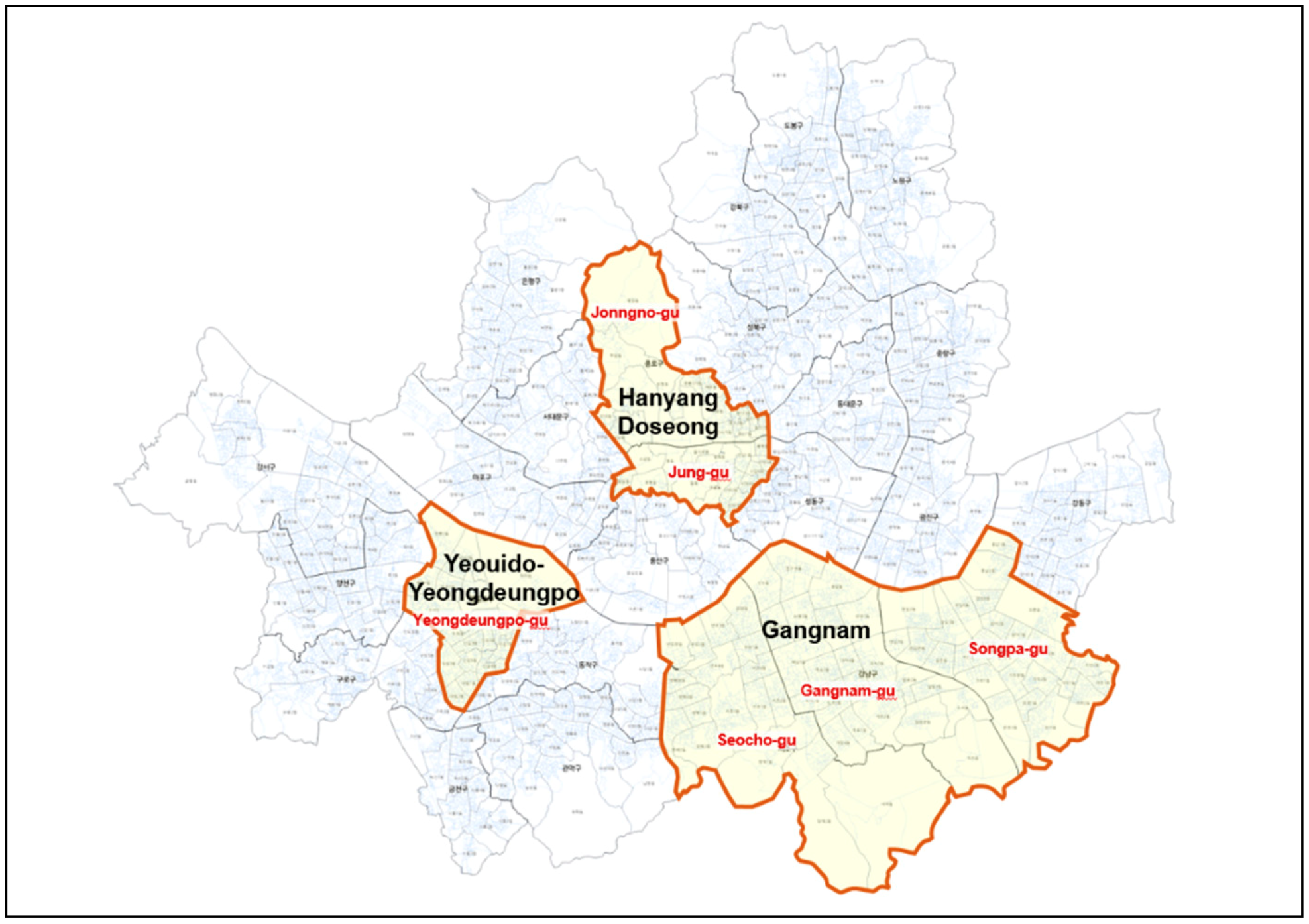
Seoul, the capital of Korea, serves as a national political, economic, and cultural center. It comprises 25 basic local governments called “gu,” which are similar to boroughs. The areas for this study are gus where the three main centers of Seoul are located. As Figure 1 illustrates, the Seoul Master Plan includes three main centers: Hanyang Doseong, Yeouido-Yeongdeungpo, and Gangnam [78]. Hanyang Doseong is a historic cultural center that is home to many historic buildings and government buildings, including Cheong Wa Dae (the Blue House) and Seoul City Hall, which spans Jongno-gu and Jung-gu. Yeouido-Yeongdeungpo is an international financial center where financial companies are concentrated, which is located at Yeongdeungpo-gu. Gangnam is an international business center with high-priced houses and commercial places popular with young people, which spans Gangnam-gu, Seocho-gu, and Songpa-gu. This study analyzed the use of space by gender for these six gus in Seoul using temporary population.
Geovision, a division of SK Telecom, which is Korea’s largest telecommunication company, provided temporary population estimates using mobile phone data. The data were collected based on a pCell measuring 50 × 50 m, which is a spatial unit that aggregates mobile phone signals, such as phone use, text messaging, and data communication, excluding Wi-Fi use. The volume of the temporary population was estimated on an hourly basis by pCell using an algorithm that Geovison developed.
Geovision released temporary population estimates for April, June, September, and December 2013 to the public to promote research through the Big Data Campus of the Seoul Metropolitan Government. It did not provide hourly data on the temporary population by gender but only daily temporary population data that summed hourly temporary population for 24 h by point, the coordinate of pCell. Daily temporary population by gender can only be aggregated by age.
We selected daily temporary population data for September, when outdoor activities occur frequently given the pleasant weather. To reduce volatility, we calculated the average of daily temporary populations, which did not target any particular age group, but represented everyone who used mobile phones. Through this process, 49,368 pCell points with daily temporary populations by gender were built as a GIS-based database. The distribution of pCell points is affected by the location of the mobile-communication repeaters of SK Telecom, which are installed with consideration of population density, topography, land use, and so on. As seen in Table 1, Gangnam-gu has the most pCell points with 23.6%, while Jung-gu has the fewest pCell points with 7.5%. By center, Gangnam Center has 65.9% of the pCell points, more than the sum of the pCell points of Hanyang Doseong Center and Yeouido-Yeongdeungpo Center.
3.2. Description of Variables
3.2.1. Dependent Variables
This study empirically examined the use of urban space and factors influencing it by gender, using daily temporary population. The total temporary population was first used as a dependent variable to understand its general characteristics. The women’s temporary population was used to derive the unique characteristics of women’s activities, and the men’s temporary population was also used to compare to that of women.
We first analyzed the pattern of temporary populations using kernel density estimation (KDE). As the distribution of the women’s temporary population was roughly similar to that of the men’s, it was not easy to derive characteristics unique to women. To overcome this problem, we additionally analyzed a relative indicator, the subtraction of men’s temporary population from women’s temporary population (SMW). If the SMW is greater than zero in a certain area, women’s activities are greater than men’s activities in that area.
Table 2 shows that the average of men’s temporary population is larger than that of women. As a result, the average of the SMW is less than zero. Given that there are not many areas where women’s temporary populations are absolutely larger than men’s, we were interested in finding areas where the SMW is relatively larger than in other areas.
3.2.2. Independent Variables
According to existing studies, women’s use of urban space differs from men’s use [46,47,79,80]. Women often use private spaces, which are areas that support family care near residential areas, while men mainly use public spaces as work spaces, which are external areas that produce social goods [79]. Women use facilities related to childcare, consumption, culture, and leisure activities more, while men use facilities related to work and entertainment more [46]. The temporary population patterns are the results of these behaviors. The capacity and suitability of an area to support such behaviors are important factors that affect the size of its temporary population. Accordingly, we examined the influences of land use and demographic characteristics, commercial and public services, and proximity of public transportation on temporary population. To do so, we established independent variables based on our expectations of differences in women’s and men’s use of urban space at the neighborhood level (i.e., variables measured by “dong”—the minimum administrative unit—and distance variables) (see Table 2). Additionally, to examine the influence of each basic local government, dummy variables using Gangnam-gu as a reference group were adopted. Gangnam-gu was used as a comparative standard because it has the largest number of companies and houses, which can influence the temporary population by generating people’s movement to and from work and home.
Regarding land use characteristics, business density and housing density of each dong were included as independent variables to represent workers’ activities and residents’ activities, respectively. Calculation of the business density includes all profit and nonprofit businesses that perform production, sales, and service activities: Stores, offices, restaurants, schools, hospitals, churches, social welfare facilities, and so on. Temporary population is expected to be large in commercial areas but small in residential areas. Particularly in Korea, women’s participation in economic activities is relatively low. The women’s labor force participation rate is 52.7%, while the men’s is 74.1%, as compared to the OECD’s average for women’s labor participation rate, 64.0% [81]. Therefore, we expected more men and fewer women in commercial areas; we also expected a lower SMW in those areas. To examine the effects of housing type, the distance from each pCell point to the nearest detached house and the distance from each pCell point to the nearest apartment house were included as independent variables. In addition, land price was included to represent land use conditions, given that land prices are generally higher in commercial areas than in residential areas.
Regarding demographic characteristics, considering that there are more women in areas with more children, the child dependency ratio was included as an independent variable. The old-age dependency ratio was also included to reflect the low activity of the elderly. The variable of population density was measured by residential population density because Korea’s official population is managed by the resident registration system. Thus, in residential areas, population density is likely to be higher than in other areas. We expected that women are relatively active in high-population-density areas.
Regarding commercial services, the distance to the nearest department store was included because women are more likely to visit department stores than men (women’s visiting rate: 29.8%; men’s: 25.9%) [82]. The floor areas of small businesses by dong were included to micro-analyze the influence of various commercial services. Small businesses mean neighborhood stores where people visit for daily needs. The types of small businesses were classified according to the Korean Standard Industrial Classification Table [83]. Clothing retailers, hair beauty shops, snack bars, and bakeries—which are expected to have a positive effect on SMW because women are generally more interested in fashion, beauty, and food than men—were included in the analysis. In addition, singing rooms, computer game rooms, and billiard rooms—which are expected to have a negative effect on SMW given that men typically visit these places more—were included.
Regarding public services, the floor areas of cultural facilities, such as theaters, music halls, assembly facilities, museums, art galleries, memorials, and libraries, were included because women typically visit cultural facilities more than men. Because women tend to have more leisure time than men in Korea and are, therefore, more likely to visit parks, we included the distance from each pCell point to the nearest park.
Public transportation is a major means of moving people on a large scale throughout Seoul. Bus stops and subway stations play an important role as centers of public transit service. Points near these facilities are expected to have a higher temporary population, whereas points farther away from these facilities are expected to have a lower temporary population. However, little is known about the effect of the gender gap on temporary populations. To examine this fact, we included the distance from each pCell point to the nearest bus stop and subway station as independent variables.
3.3. Methods
This study examined influencing factors for three kinds of temporary populations: Total, women’s, and men’s temporary populations. SMW was also analyzed to understand the differences in women’s and men’s activities.
The ordinary least squares (OLS) method was used as a basic model to examine the relationship between temporary populations and independent variables. OLS regression can be written as follows:
where is an vector of observations on temporary populations as a dependent variable; is an matrix of observations on independent variables; is a vector of regression coefficients to be estimated; and is the vector of error terms with
The temporary population data are likely to have spatial autocorrelation in that the data are built based on pCell points that have similar location conditions when they are adjacent to each other. Spatial autocorrelation refers to the correlation among values of a single variable that is strictly attributable to their relatively close locational positions on a two-dimensional surface [84]. The positive spatial autocorrelation shows that high values tend to be close to high values and low values tend to be close to low values. Spatial autocorrelation is usually analyzed by using Moran’s I. If the positive spatial autocorrelation exists in the data, local clustering is generally observed. Local clustering can be effectively mapped using the local indicators of spatial association (LISA) suggested by Anselin [85].
OLS regression does not consider spatial autocorrelation. Therefore, we used the spatial regression model to consider spatial autocorrelation. This model has several forms, but two forms are generally used: The spatial lag model (SLM) and the spatial error model (SEM). SLM assumes that spatial autocorrelation exists among values of a dependent variable. It is formulated as follows:
where , and are the same as in the OLS regression; is the spatial weight matrix; and is a spatial autoregression coefficient.
The SEM assumes that there is a spatial autocorrelation among residuals. The SEM is formulated as follows:
where , and are the same as in the SLM regression; is a spatial autoregression coefficient of the residuals; and is an vector of residuals. The SLM and SEM estimate parameters using the maximum likelihood method.
In general, model selection is determined by the Lagrange Multiplier (LM) test. If the LM-Lag statistic is significant, SLM is selected, and if the LM-Error statistic is significant, SEM is selected. If both statistics are significant, model selection is determined by comparing the Robust LM-Lag statistic and Robust LM-Error statistic in the Robust LM test. The goodness of fit of the models can be compared using the Log Likelihood (LogL), Akaike Information Criterion (AIC), and Schwarz Criterion (SC). An increase in LogL decreases AIC and SC, which means that the goodness of fit of the model is improved.
4. Results
4.1. Kernel Density Analysis
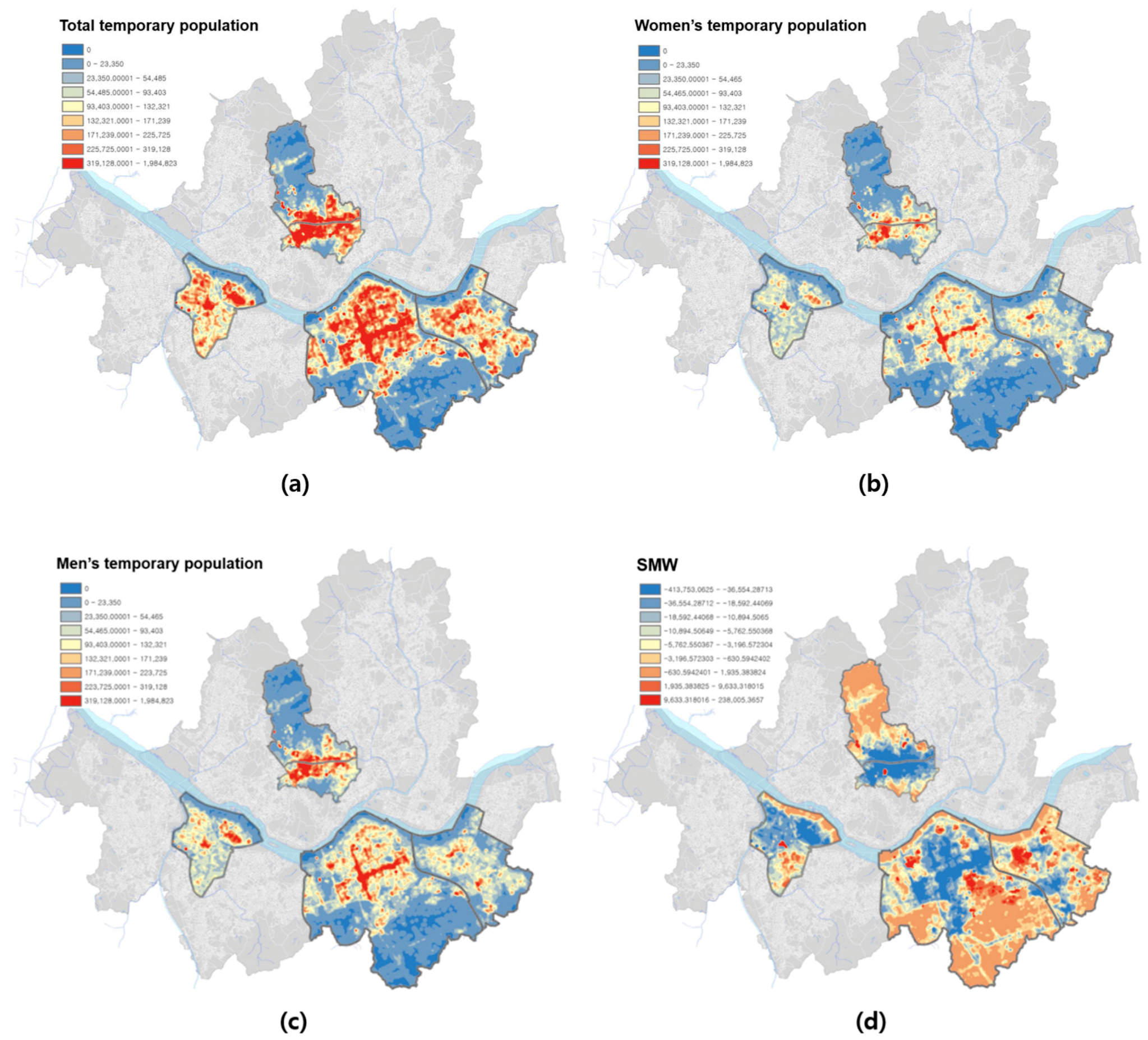
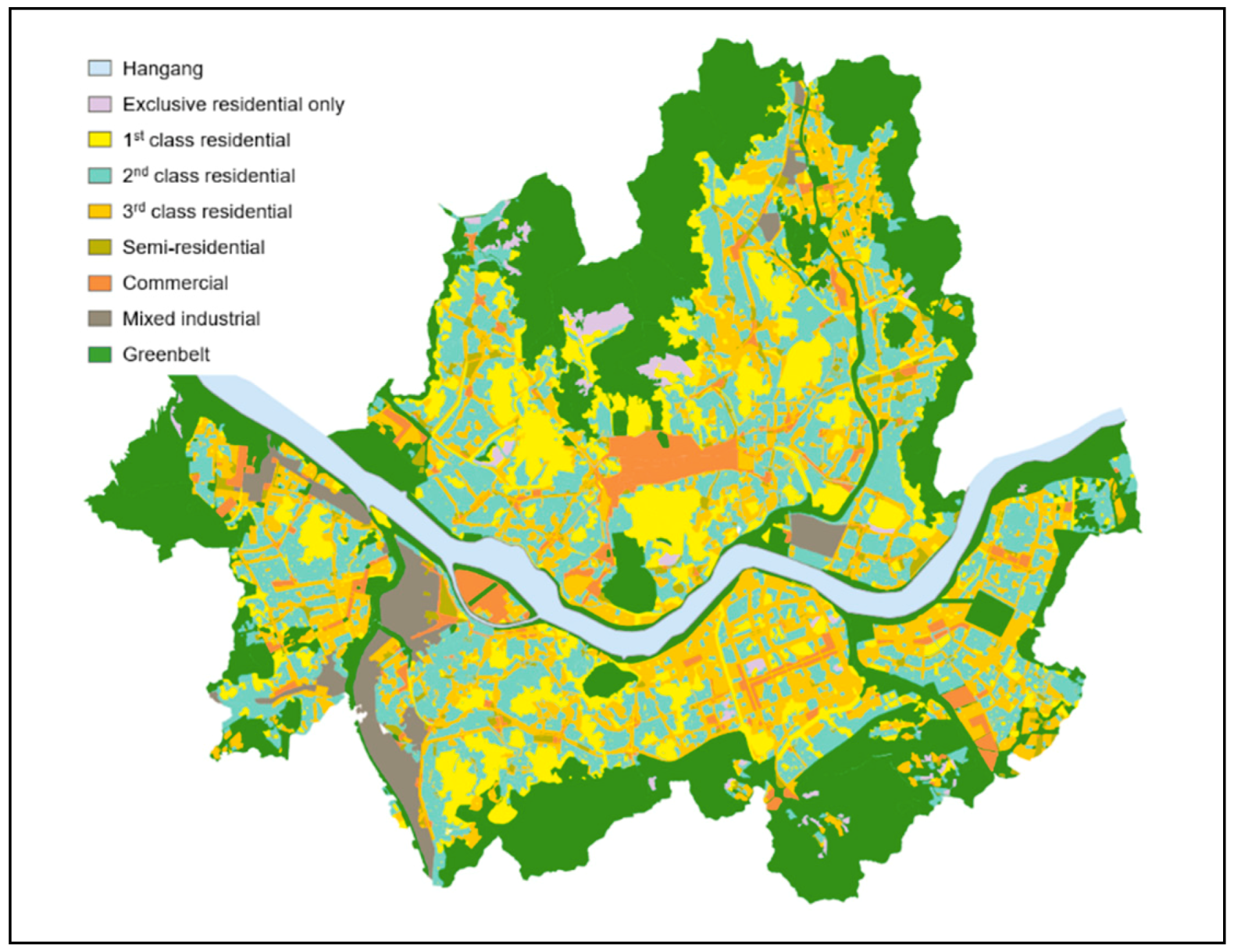
To analyze the patterns of temporary populations, kernel density mapping was performed using KDE of ArcGIS. As shown in Figure 2, the deeper the red color, the larger the temporary population was, and the deeper the blue color, the smaller the temporary population was. Regarding SMW, the deeper the red color, the more active women’s use of space was than men’s, and the deeper the blue color, the less active women’s use of space was. Figure 3 is a zoning map that shows land use patterns of Seoul. By comparing Figure 2 and Figure 3, we found the relationship between temporary population and land use.
The results of kernel density analysis are summarized as follows. First, patterns of women’s and men’s temporary populations were similar. Generally, they were large in commercial areas and small in residential areas. Therefore, the women’s temporary population alone has limitations in terms of deriving gender gap characteristics. Second, SMW showed a pattern that is almost the inverse of the total temporary population pattern. Women were relatively more active in residential and green areas than in commercial areas, while men were more active in commercial areas than in residential areas. Most areas where women outnumbered men were areas with small temporary populations or residential areas. This result might reflect the tendency of women to stay near their residential areas. Third, SMW, a relative indicator, tended to be the inverse of the total temporary population, an absolute indicator, but not in all areas. Among the areas with a large temporary population, there were areas where the women’s temporary populations were larger than men’s. This phenomenon was noticeable near areas where department stores are located.
The overall patterns of total, women’s, and men’s temporary populations were examined through kernel density. As the spatial pattern of women’s temporary populations was generally similar to that of men’s and total temporary populations, it was difficult to derive the unique characteristics of the temporary population pattern of women when analyzed separately. However, SMW showed relatively prominent characteristics for women’s use of urban space by focusing on the differences in women’s and men’s temporary populations. Despite these results, an analysis that relies solely on the visualization of data may be subjective, and thus, it was necessary to specifically verify our expectations of women’s use of urban space through empirical analysis using statistical models.
4.2. Spatial Autocorrelation
4.2.1. Moran’s I
A spatial weighted matrix was first established to analyze the spatial autocorrelation of temporary populations. Two criteria, spatial contiguity and spatial distance, are generally used to establish a spatial weighted matrix. We used the threshold distance method, which is a type of spatial contiguity that identifies all points in the threshold distance as spatial neighbors. All points were located at the intersection of a 50 × 50 m grid. The threshold distance was set to 70.8 m, slightly larger than m, to include four points in the diagonal direction as well as four points in the vertical and horizontal directions.
Moran’s I was applied to the spatial weighted matrix to analyze the spatial autocorrelation of temporary populations. Values of Moran’s I measured by the ArcGIS program ranged from 0.41 to 0.57 (Table 3). These results showed that all of the temporary population data had spatial autocorrelation. In particular, SMW had the highest value of 0.57, indicating strong spatial autocorrelation.
4.2.2. Local Indicators of Spatial Association
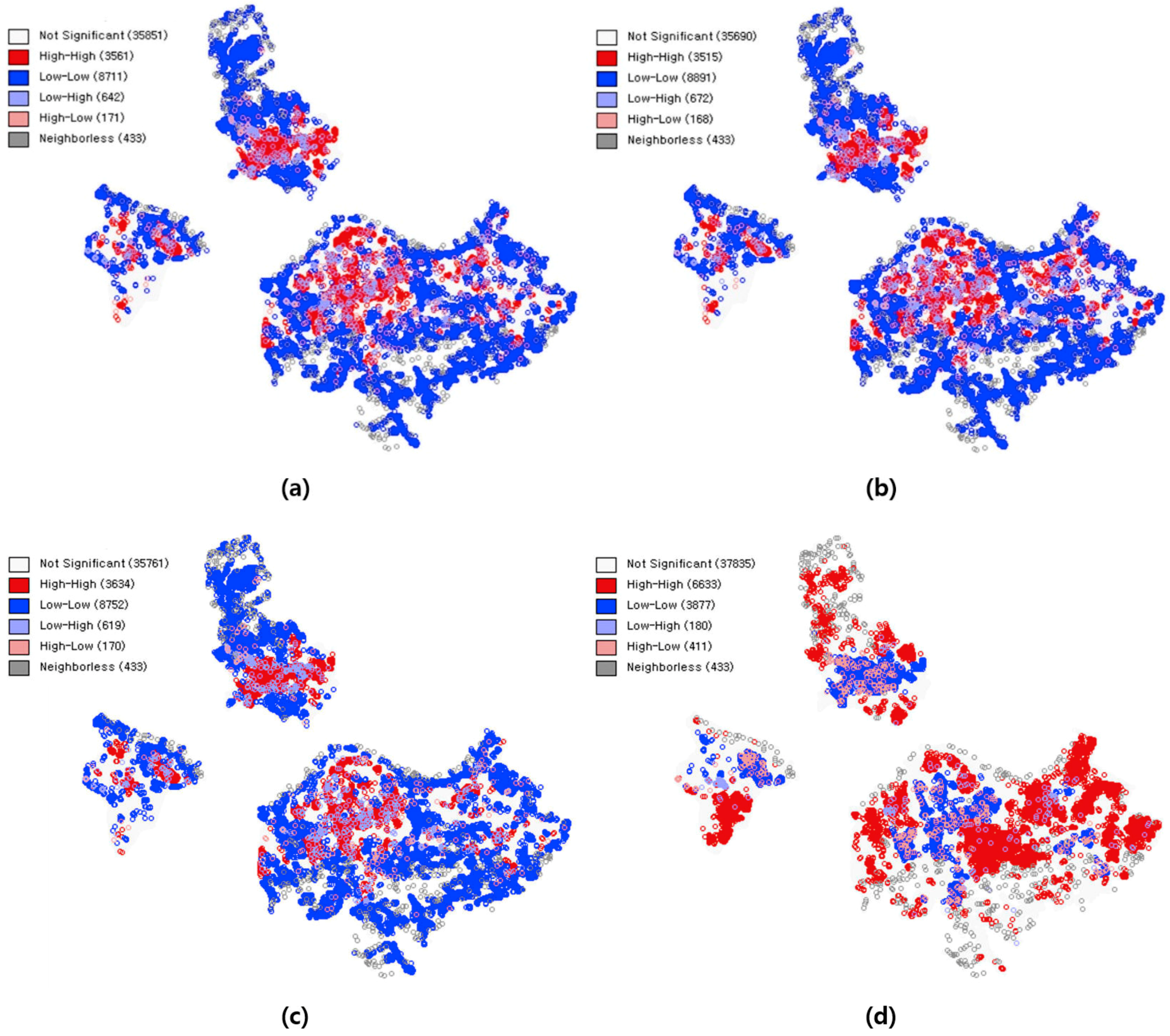
LISA maps using the GeoDA program are shown in Figure 4. When the value of a point and the values of the points surrounding it are high together, the point appears in red, and when the value of a point and the values of the points surrounding it are low together, the point appears in blue. The LISA maps of total, women’s, and men’s temporary populations are similar.
Red points were clustered in the commercial areas of Hanyang Doseong, Yeouido-Yeongdeungpo, and Gangnam centers; blue points were prominent in residential areas on the outskirts of all three centers. SMW had a different pattern from the total, women’s, and men’s temporary populations. The LISA pattern of SMW was characterized by red points prominent in residential areas and blue points clustered in commercial areas. This pattern is almost the inverse of the total, women’s, and men’s temporary populations.
4.3. Results of Spatial Regression Analysis
From the results of the spatial autocorrelation analysis previously conducted, we confirmed that temporary populations had spatial autocorrelation. Therefore, the two spatial regression models that can consider spatial autocorrelation, the SLM and SEM, were used for the analysis.
Applying OLS to the four temporary populations, we found that the statistics of the LM test were all significant, and thus, the introduction of the spatial regression model is valid. However, because the results of the robust LM tests were all significant, model selection became difficult (see Table A1). Therefore, we attempted to select the most appropriate model by comparing the goodness of fit. In all four models, the SLM had the largest LogL and the smallest AIC and SC, and thus, we selected the SLM as the most appropriate model (see Table 3, Table A1 and Table A2).
Going forward, the SLM is used to describe the relationship between dependent and independent variables. The results of the SLM are shown in Table 4. Spatial autoregression coefficients () were significant for all models, confirming that the total, women’s, and men’s temporary populations as well as the SMW data had spatial autocorrelation, which means that there existed local clustering phenomena, as shown in the LISA cluster maps of Figure 4. In other words, this means that areas located around areas with large temporary populations tended to have large temporary populations. From the perspective of urban planning for gender equality, clustered patterns in the women’s temporary population and SMW have important meanings in that clustered patterns make it easier to support women’ needs in planning land use and facilities than scattered patterns.
When looking at local dummy variables, it is important to recall that Gangnam-gu is a reference group and that the value of the dependent variable is the daily temporary population of each point. Looking only at signs of estimated coefficients, Jongno-gu, Jung-gu, and Yeongdeungpo-gu were larger for the women’s temporary population than Gangnam-gu but smaller for the SMW, while Seocho-gu and Songpa-gu were smaller for the women’s temporary population but larger for the SMW. This pattern was closely related to population distribution. Each gu’s population ratio compared to total population is as follows: Songpa-gu, 28.5%; Gangnam-gu, 23.2%; Seocho-gu, 18.6%; Yeongdeungpo-gu, 17.1%; Jongno-gu, 6.9%; and Jung-gu, 5.7%. The gus with large populations have large residential areas, which might have a negative effect on the women’s temporary population similar to men’s, but a positive effect on the SMW. The coefficients of Songpa-gu, which has a larger population than Gangnam-gu, had the opposite signs of those of Yeongdeungpo-gu, which has a smaller population. Furthermore, this explanation may also apply to comparisons between centers. Women’s temporary populations of Hanyang Doseong and Yeouido-Yeongdeungpo are larger than that of Gangnam, while the SMWs of Hanyang Doseong and Yeouido-Yeongdeungpo are smaller. This pattern is also attributed to the fact that the population of Gangnam is larger than those of the other centers: Gangnam, 70.3%; Yeouido-Yeongdeungpo, 17.1%; and Hanyang Doseong, 12.6%. However, the above explanation has limitations in that some gus (i.e., Jung-gu and Seocho-gu) were not significant with respect to the women’s temporary population and others (i.e., Jongno-gu and Seocho-gu) were not with respect to the SMW.
According to the analysis of land use characteristics, business density had a positive effect on the women’s temporary population, as well as on the total and men’s temporary populations, and a negative effect on SMW. Housing density had negative effects on total, women’s, and men’s temporary populations, but the effects were not significant. Nevertheless, housing density had a positive effect on SMW. Considering that business density and housing density represent workers’ and residents’ activities, respectively, the results showed that women are more in the commercial area, like men, but less in the commercial area and more in the residential area. Distance to detached house was not significant, while distance to apartment was significant in all models. Apartments are located in large-scale residential areas that have strong residential characteristics, but detached houses are often found in residential areas mixed with commercial use, which likely affected the results. Land price had positive effects on total, women’s, and men’s temporary populations, but a negative effect on SMW, which was the same as business density, but the opposite of housing density. This might be because land prices are generally higher in commercial areas than in residential areas.
Regarding the effect of demographic characteristics, an increase in population density influenced an increase in the women’s temporary population and SMW. Population density was higher in residential areas with more residents, and this positively affected the women’s temporary population and SMW. Child dependency ratio was not significant for the total, women’s, or men’s temporary populations. Nevertheless, it had a positive effect on SMW, which is related to the fact that women are more in charge of childcare than men. An increase in old-age dependency ratio was attributed to a decrease of all temporary populations, including SMW. Because the elderly are less mobile and use cell phones with less frequency, the more elderly were in a location, the lower the temporary population.
According to the analysis of commercial services, distance to department store had no significant influence on the women’s temporary population, but had a significant influence on the total and men’s temporary populations as well as SMW. Distance to department store had a negative effect on SMW because the men’s temporary population decreased as a department store became closer. This result confirmed our expectations. Regarding small businesses, significant variables for the women’s model are interpreted as follows: Clothing retailers, bakeries, singing rooms, and computer game rooms had positive effects, while supermarkets and hair beauty shops had negative effects. Different results appeared for SMW: Clothing retailers, hair beauty shops, and snack bars, which are closely related to women’s activities, had positive effects, while real estate brokerages, singing rooms, computer game rooms, and billiard rooms, which are largely men’s activities, had negative effects.
According to the analysis of public services, the density of cultural facilities, which was closely tied to women’s activities, had a significantly negative effect on the total and men’s temporary populations, but a significantly positive effect on SMW. As parks were generally located close to residential areas, the increase in distance to park increased the total, women’s, and men’s temporary populations, but decreased SMW.
According to the analysis of public transit proximity, both the distance to bus stop and distance to subway station had significantly negative effects on the total, women’s, and men’s temporary populations. However, they had positive effects on SMW, which was closely tied to the fact that men are more active near bus stops and subway stations.
5. Discussion
The results of the analyses demonstrated the effects of two conflicting ideologies (or trends) related to the gender roles discussed in the literature review (Section 2.1.1): One is the increase in women’s inflow into the public domain and the spread of gender-egalitarian attitudes [26], and the other is the continuing influence of traditional gender role ideology [27]. This study was able to observe the influences of both trends by using absolute and relative indicators together: Total, men’s, and women’s temporary populations as absolute indicators, and SMW as a relative one. On one hand, temporary population patterns for the total, women, and men showed similar patterns in that both men’s and women’s temporary populations were larger in business areas and smaller in residential areas, which infers that a large number of women, like men, are participating in economic activities. These results are consistent with existing studies dealing with the changes in the women’s labor market in Korea [28,29]. On the other hand, SMW, a relative indicator, showed the opposite patterns of the absolute indicators described above, reflecting the influence of traditional gender role ideology emphasizing women’s responsibilities in household affairs. SMW was larger in residential areas and smaller in business areas. This result is in line with the results of Son’s study, which state that married women with children are less mobile due to their high responsibility for household chores [43].
Among the above indicators used in this study, SMW is particularly noteworthy. We confirmed the usefulness of SMW with the following results. The kernel density patterns and the signs of coefficients of the SLM for women’s and men’s temporary populations were quite similar, and, therefore, it was difficult to identify women’s use patterns of urban spaces from that analysis. However, the analyses of SMW demonstrated where women were relatively more active by focusing on the differences between women’s and men’s activities. Particularly, we found gender differences in the use of urban space at the local and neighborhood levels, which were in line with existing studies examining gender differences related to urban spaces [37,42,43,44,80]. At the local level, the women’s temporary populations in Hanyang Doseong and Yeouido-Yeongdeungpo were larger than in Gangnam, while SMW was larger in Gangnam than in Hanyang Doseong and Yeouido-Yeongdeungpo; this is likely because Gangnam has more residential areas than the other locations, and, therefore, more women’s activities are expected in Gangnam. At the neighborhood level, women’s activities appeared in the following ways, depending on the characteristics of neighborhoods. Similar to men’s temporary population, the women’s temporary population was large in business districts and near subway stations, but small in residential areas. However, SMW demonstrated the subtle differences between where women’s and men’s activities occurred; SMW was larger in areas with more dwellings, more children, and more neighborhood retail, such as clothing stores, beauty shops, and restaurants, as well as closer to parks, department stores, and cultural facilities. These results affirm Garcia-Ramon’s statement that women “spend more time outdoors, carrying out tasks which are mostly related to family affairs and domestic work” [87] (p. 216), and also coincide with the results of Korean studies that uncovered women’s preference for urban spaces related to upbringing and leisure [37,44]. However, as Son’s study suggested [43], such results might be caused by socially formed gender roles rather than biological sex. Son revealed in her study analyzing survey data about mobility in Seoul that married women with children had less mobility than men in urban spaces, while unmarried working women had the same or even higher mobility than men.
In addition, both women’s temporary populations and SMW had spatial autocorrelation and, therefore, showed clustering patterns (see the LISA cluster map in Figure 4). This is an improved result from the result of Yun et al.’s study [60] analyzing temporary population survey data and demonstrating that temporary populations had spatial correlation, in that this study conducted a more accurate analysis with 49,368 data points, while Yun et al. used 10,000 data points. In terms of urban planning for gender equality, clustered patterns of women’s temporary populations and SMW have important meanings, particularly with regard to practical approaches for gender-egalitarian planning, as Sandercock and Forsyth suggested [11]. That is, clustered patterns make it easier to support women’s present needs in planning land use and facilities than do scattered patterns. A strategic approach that aims for a fundamental change of social structure that produces gender inequality may require more than physical planning to satisfy present needs.
6. Conclusions
In this study, we examined gender gaps in the use of urban space in Seoul, Korea to provide empirical evidence for urban planning for gender equality. We analyzed daily temporary populations collected from mobile phone data. We used the total, women’s, and men’s temporary populations and SMW as dependent variables, with a particular focus on the women’s temporary population and SMW, which subtracts men’s temporary population from women’s temporary population. We first made a visual analysis of temporary population density using KDE, and conducted further analysis using spatial autocorrelation indicators and spatial regression models.
The key findings are summarized as follows. First, temporary population patterns for women and men showed similar patterns in that both temporary populations were larger in business areas than in residential areas, which means that, like men, a large number of women are engaged in economic activities. Second, the pattern for SMW showed the opposite patterns, that is, women were more active in residential areas and areas easily accessible to neighborhood retail shops, cultural facilities, parks, and department stores. Finally, both women’s temporary populations and SMWs had spatial autocorrelation and, thus, showed clustering patterns.
This study contributes to urban planning for gender equality in Korea by analyzing how gender-specific differences occur in space use, explaining spatial patterns, and deducing the causes of such differences. This study has the same limitations related to representativeness of data and different patterns of mobile phone use as other studies analyzing mobile phone data. As Gauvin warned, first, data may not be representative of the population being studied due to the market share of the telecommunication company providing the data; second, people’s patterns of use of space are inferred through their patterns of mobile phone use [80]. Further studies analyzing mobile phone data from other telecommunication companies may contribute to addressing the issues related to the former limitation, and those analyzing temporary population collected by field survey may help solve the latter limitation. The study also has another limitation related to data. Geovision collected mobile phone data on an hourly basis, but released limited data compiled on a daily basis to the public. Therefore, we could not analyze space usage patterns by gender on an hourly basis. However, the Korean government is demanding that private telecommunications companies release more and more information to the public, so it is expected that it will be possible to analyze hourly data in the near future. Finally, this study, as an exploratory study, analyzed the overall patterns of space use by gender observed at local and neighborhood levels, and gave little consideration to the detailed spatial qualities each place has. However, such spatial qualities must also be considered in order to propose practical urban policy alternatives for public spaces, and future studies focusing on a specific place and analyzing the spatial qualities of that place may complement such a limitation.
Author Contributions
A.J., S.-K.L., and J.K. led and contributed equally to this research—conceptualization, A.J. and J.K.; methodology, S.-K.L.; formal analysis, A.J. and S.-K.L.; investigation, A.J.; data curation, A.J.; writing—original draft preparation, A.J., S.-K.L., and J.K.; visualization, A.J. and J.K.; supervision, S.-K.L. All authors have read and agreed to the published version of the manuscript.
Funding
This research received no external funding.
Conflicts of Interest
The authors declare no conflict of interest.
Appendix A

Table A1.
Analysis results of ordinary least squares (OLS) regression.
| Variable | Total | Women’s | Men’s | SMW | ||||
|---|---|---|---|---|---|---|---|---|
| Coef. | t | Coef. | t | Coef. | t | Coef. | t | |
| Constant | 295.84 *** | 10.11 | 158.41 *** | 9.82 | 136.41 *** | 10.17 | −21.62 *** | −4.46 |
| Jongno-gu | 74.35 *** | 5.39 | 36.64 *** | 4.82 | 37.67 *** | 5.96 | 1.04 | 0.46 |
| Jung-gu | 41.60 *** | 2.65 | 27.82 *** | 3.21 | 13.84 * | 1.92 | −14.00 *** | −5.37 |
| Yeongdeungpo-gu | 34.10 *** | 2.83 | 20.18 *** | 3.04 | 13.99 ** | 2.53 | −6.22 *** | −3.11 |
| Seocho-gu | −24.01 ** | −2.37 | −14.47 *** | −2.60 | −9.56 ** | −2.06 | 4.92 *** | 2.94 |
| Songpa-gu | −111.29 *** | −9.92 | −64.57 *** | −10.45 | −46.69 *** | −9.07 | 17.87 *** | 9.60 |
| Business density | −0.91 ** | −2.19 | −0.59 ** | −2.57 | −0.32 * | −1.69 | −67.7 *** | −23.53 |
| Housing density | 0.02 | 1.08 | 0.01 | 0.91 | 0.01 | 1.21 | 0.27 *** | 3.85 |
| Distance to detached house | 0.13 ** | 5.90 | 0.08 *** | 6.71 | 0.05 *** | 4.81 | 0.001 | 0.34 |
| Distance to apartment | 47.45 *** | 31.45 | 28.05 *** | 33.75 | 19.42 *** | 28.07 | −0.03 *** | −8.99 |
| Land price | −1.05 | −1.30 | −0.97 ** | −2.19 | −0.06 | −0.17 | −8.63 *** | −34.51 |
| Population density | −5.55 *** | −5.11 | −2.34 ** | −3.90 | −3.18 *** | −6.39 | 11.32 *** | 18.13 |
| Child dependency ratio | 333.42 *** | 19.22 | 200.55 *** | 20.99 | 132.82 *** | 16.69 | 0.91 *** | 6.76 |
| Old-age dependency ratio | 7.54 ** | 2.00 | −1.89 | −0.91 | 9.42 *** | 5.46 | −0.86 *** | −4.77 |
| Distance to department store | 0.15 ** | 2.23 | −0.02 | −0.45 | 0.17 *** | 5.37 | −3.07 *** | −6.03 |
| Clothing retails | 5.08 *** | 4.60 | 3.76 *** | 6.17 | 1.34 *** | 2.63 | 0.19 *** | 16.36 |
| Real estate brokerages | −16.45 *** | −7.98 | −8.26 *** | −7.28 | −8.18 *** | −8.65 | −2.43 *** | −13.24 |
| Supermarkets | −2.83 *** | −4.56 | −1.86 *** | −5.44 | −0.97 *** | −3.40 | 0.08 | 0.24 |
| Hair beauty shops | −4.29 | −1.19 | −5.20 *** | −2.61 | 0.96 | 0.58 | 0.89 *** | 8.66 |
| Snack bars | 11.78 *** | 8.85 | 5.76 *** | 7.85 | 6.02 *** | 9.86 | 6.14 *** | 10.25 |
| Bakeries | 5.50 *** | 4.27 | 3.18 *** | 4.49 | 2.33 *** | 3.95 | 0.26 | 1.20 |
| Singing rooms | 12.55 *** | 5.19 | 7.23 *** | 5.43 | 5.35 *** | 4.83 | −0.85 *** | −4.00 |
| Computer game rooms | 1.15 | 0.65 | 2.86 *** | 2.90 | −1.71 ** | −2.08 | −1.89 *** | −4.70 |
| Billiard rooms | 7.08 ** | 2.31 | 5.08 *** | 3.00 | 2.02 | 1.43 | −4.56 *** | −15.39 |
| Density of cultural facilities | −4.46 * | −1.87 | −6.01 *** | −4.59 | 1.56 | 1.43 | 7.57 *** | 19.20 |
| Distance to park | 73.93 *** | 3.61 | 51.14 *** | 4.53 | 22.83 ** | 2.43 | −28.33 *** | −8.33 |
| Distance to bus stop | −315.88 *** | −18.16 | −174.98 *** | −18.27 | −140.95 *** | −17.67 | 34.05 *** | 11.80 |
| Distance to subway station | −63.05 *** | −11.63 | −36.69 *** | −12.29 | −26.33 *** | −10.59 | 10.36 *** | 11.52 |
| R-squared | 0.13 | 0.14 | 0.12 | 0.18 | ||||
| N | 49,368 | 49,368 | 49,368 | 49,368 | ||||
| Log likelihood | −388,381 | −358,936 | −349,904 | −299,678 | ||||
| AIC | 776,818 | 717,927 | 699,865 | 599,411 | ||||
| SC | 777,065 | 718,174 | 700,111 | 599,658 | ||||
| LM-Lag | 11,887.5 *** | 12,871.3 *** | 10,927.2 *** | 19,054.4 *** | ||||
| LM-Error | 11,696.1 *** | 12,650.2 *** | 10,763.5 *** | 18,618.7 *** | ||||
| Robust LM-Lag | 206.2 *** | 235.6 *** | 178.9 *** | 452.0 *** | ||||
| Robust LM-Error | 14.7 *** | 14.5 *** | 15.2 *** | 16.3 *** | ||||
Notes: * p < 0.1; ** p < 0.05; *** p < 0.01.
Table A2.
Analysis results of spatial error model (SEM).
| Variable | Total | Women’s | Men’s | SMW | ||||
|---|---|---|---|---|---|---|---|---|
| Coef. | z | Coef. | z | Coef. | z | Coef. | z | |
| Constant | 367.82 | 7.94 | 162.31 *** | 7.75 | 201.41 *** | 7.78 | −40.17 *** | −4.79 |
| Jongno-gu | 77.41 *** | 3.38 | 37.71 *** | 3.65 | 39.78 *** | 3.10 | −3.52 | −0.83 |
| Jung-gu | 59.13 *** | 2.25 | 20.33 * | 1.72 | 39.40 *** | 2.68 | −19.96 *** | −4.08 |
| Yeongdeungpo-gu | 17.56 | 0.87 | 7.65 | 0.84 | 10.40 | 0.92 | −2.70 | −0.72 |
| Seocho-gu | −12.59 | −0.74 | −5.04 | −0.66 | −7.57 | −0.79 | 2.58 | 0.81 |
| Songpa-gu | −105.52 *** | −5.58 | −43.25 *** | −5.08 | −62.20 *** | −5.87 | 20.06 *** | 5.67 |
| Business density | 305.43 *** | 11.03 | 123.5 *** | 9.87 | 181.49 *** | 11.74 | −55.93 *** | −11.15 |
| Housing density | −0.16 | −0.34 | −0.05 | −0.25 | −0.10 | −0.39 | 0.03 | 0.44 |
| Distance to detached house | 0.02 | 0.95 | 0.01 | 0.96 | 0.01 | 0.90 | −0.002 | −0.46 |
| Distance to apartment | 0.13 *** | 3.64 | 0.05 *** | 3.08 | 0.08 *** | 4.01 | −0.03 *** | −4.49 |
| Land price | 41.53 *** | 18.12 | 17.22 *** | 16.56 | 24.32 *** | 19.05 | −6.94 *** | −17.10 |
| Population density | 9.9 | 1.63 | 9.81 *** | 3.58 | 0.14 | 0.04 | 8.93 *** | 8.09 |
| Child dependency ratio | −1.54 | −1.18 | −0.25 | −0.42 | −1.20 | −1.63 | 0.93 *** | 3.89 |
| Aged dependency ratio | −6.33 *** | −3.70 | −3.31 *** | −4.28 | −2.91 *** | −3.05 | −0.27 | −0.88 |
| Distance to department store | −0.67 | −0.13 | −1.3 | −0.56 | 0.67 | 0.23 | −2.19 | −2.28 |
| Clothing retails | 0.08 | 0.73 | 0.12 ** | 2.48 | −0.04 | −0.72 | 0.15 *** | 7.51 |
| Real estate brokerages | 3.13 ** | 1.99 | 0.79 | 1.11 | 2.35 *** | 2.69 | −1.36 *** | −5.05 |
| Supermarkets | −14.82 *** | −4.55 | −7.49 *** | −5.08 | −7.33 *** | −4.03 | −0.07 | −0.11 |
| Hair beauty shops | −2.6 *** | −2.58 | −0.92 ** | −2.01 | −1.67 *** | −2.96 | 0.70 *** | 3.79 |
| Snack bars | −5.36 | −0.94 | 0.36 | 0.14 | −5.52 ** | −1.74 | 5.63 *** | 5.51 |
| Bakeries | 10.47 *** | 4.98 | 5.4 *** | 5.68 | 5.08 *** | 4.33 | 0.17 | 0.45 |
| Singing rooms | 5.03 ** | 2.43 | 2.2 ** | 2.36 | 2.86 ** | 2.48 | −0.58 | −1.55 |
| Computer game rooms | 8.99 ** | 2.35 | 3.94 ** | 2.28 | 5.19 ** | 2.43 | −1.25 | −1.81 |
| Billiard rooms | 0.26 | 0.09 | −2.03 | −1.57 | 2.27 | 1.42 | −4.24 *** | −8.16 |
| Density of cultural facilities | −5.89 * | −1.78 | −0.04 | −0.03 | −5.76 *** | −3.14 | 4.97 *** | 8.81 |
| Distance to park | 72.77 ** | 2.16 | 24.01 | 1.58 | 48.58 *** | 2.58 | −22.97 *** | −3.70 |
| Distance to bus stop | −297.1 *** | −10.60 | −131.67 *** | −10.41 | −165.63 *** | −10.57 | 35.21 *** | 6.88 |
| Distance to subway station | −66.35 *** | −7.36 | −27.49 *** | −6.77 | −38.78 *** | −7.68 | 11.36 *** | 6.80 |
| Lambda () | 0.49 *** | 99.25 | 0.48 *** | 94.60 | 0.51 *** | 103.94 | 0.59 *** | 133.34 |
| R-squared | 0.32 | 0.30 | 0.34 | 0.45 | ||||
| N | 49,368 | 49,368 | 49,368 | 49,368 | ||||
| Log likelihood | −83,774 | −345,658 | −353,958 | −292,308 | ||||
| AIC | 767,605 | 691,372 | 707,973 | 584,672 | ||||
| SC | 767,851 | 691,619 | 708,219 | 584,919 | ||||
Notes: * p < 0.1; ** p < 0.05; *** p < 0.01.
References
- Inglehart, R.F.; Norris, P.; Welzel, C. Gender equality and democracy. Comp. Sociol. 2002, 1, 235–264. Available online: https://ssrn.com/abstract=2391796 (accessed on 1 June 2020). [CrossRef] [Green Version]
- Miotto, G.; Polo López, M.; Rom Rodríguez, J. Gender equality and UN sustainable development goals: Priorities and correlations in the top business schools’ communication and legitimation strategies. Sustainability 2019, 11, 302. [Google Scholar] [CrossRef] [Green Version]
- International Labor Office. ABC OF Women Workers’ Rights and Gender Equality, 2nd ed.; International Labor Office: Geneva, Switzerland, 2007; ISBN 978-9221196228. Available online: https://www.ilo.org/wcmsp5/groups/public/---dgreports/---gender/documents/publication/wcms_087314.pdf (accessed on 1 June 2020).
- World Economic Forum. The Global Gender Gap Report 2020; World Economic Forum: Geneva, Switzerland, 2020; ISBN 13 978-2-940631-03-2. Available online: http://www3.weforum.org/docs/WEF_GGGR_2020.pdf (accessed on 3 June 2020).
- Cook, C.C.; Andrew, C.; Bruin, M.; Garber, J.A. Gendering the City: Women, Boundaries, and Visions of Urban Life; Rowman & Littlefield: Lanham, ML, USA, 2000; ISBN 978-0847694518. [Google Scholar]
- Greed, C. Promise or progress: Women and planning. Built Environ. (1978-) 1996, 22, 9–21. Available online: https://0-www-jstor-org.brum.beds.ac.uk/stable/23287762 (accessed on 1 June 2020).
- Jaeckel, M.; Geldermalsen, M.V. Gender Sensitive Planning. In Proceedings of the Urbanism & Gender: A Necessary Vision for All, Barcelona, Spain, 27–29 April 2005; Available online: https://www.diba.cat/documents/540797/544667/seep-fitxers-urbanismgender-pdf.pdf (accessed on 29 June 2020).
- Hayden, D. What would a non-sexist city be like? Speculations on housing, urban design, and human work. J. Women Cult. Soc. 1980, 5, S170–S187. [Google Scholar] [CrossRef]
- Wekerle, G.R. A woman’s place is in the city. Antipode 1985, 17, 145–153. [Google Scholar] [CrossRef]
- Bondi, L. Gender, class, and urban space: Public and private space in contemporary urban landscapes. Urban Geogr. 1998, 19, 160–185. [Google Scholar] [CrossRef]
- Sandercock, L.; Forsyth, A. A gender agenda: New directions for planning theory. J. Am. Plan. Assoc. 1992, 58, 49–59. [Google Scholar] [CrossRef]
- Beebeejaun, Y. Gender, urban space, and the right to everyday life. J. Urban Aff. 2017, 39, 323–334. [Google Scholar] [CrossRef] [Green Version]
- Buvinic, M.; Levine, R. Closing the gender data gap. Significance 2016, 13, 34–37. [Google Scholar] [CrossRef]
- Crane, R. Is there a quiet revolution in women’s travel? Revisiting the gender gap in commuting. J. Am. Plan. Assoc. 2007, 73, 298–316. [Google Scholar] [CrossRef] [Green Version]
- Crane, R.; Takahashi, L. Sex changes everything: The recent narrowing and widening of travel differences by gender. Public Work. Manag. Policy 2009, 13, 328–337. [Google Scholar] [CrossRef]
- Farré, L.; Jofre-Monseny, J.; Torrecillas, J. Commuting Time and the Gender Gap in Labor Market Participation; Institution for the Study of Labor (IZA): Bonn, Germany, 2020. [Google Scholar]
- Charles-Edwards, E. The Estimation of Temporary Populations in Australia. In Demography for Planning and Policy: Australian Case Studies; Springer: Cham, Switzerland, 2016; pp. 31–49. [Google Scholar]
- Panczak, R.; Charles-Edwards, E.; Corcoran, J. Estimating temporary populations: A systematic review of the empirical literature. Palgrave Commun. 2020, 6, 1–10. [Google Scholar] [CrossRef]
- Smith, S.K. Toward a methodology for estimating temporary residents. J. Am. Stat. Assoc. 1989, 84, 430–436. [Google Scholar] [CrossRef]
- IT Statistics of Korea. Available online: http://www.itstat.go.kr/home.it (accessed on 11 June 2020).
- Freedman, E. No Turning Back: The History of Feminism and the Future of Women; Ballantine Books: New York, NY, USA, 2007. [Google Scholar]
- Inter-Parliamentary Union. Participation of Women in Political Life; IPU: Geneva, Switzerland, 1999. [Google Scholar]
- Butler, J. Sex and Gender in Simone de Beauvoir’s Second Sex. Yale Fr. Stud. 1986, 72, 35–49. [Google Scholar] [CrossRef]
- Cott, N.F. No Small Courage: A History of Women in the United States; Oxford University Press: New York, NY, USA, 2000. [Google Scholar]
- Eisenstein, H. Contemporary Feminist Thought; Unwin Paperbacks: London, UK, 1984. [Google Scholar]
- Shorrocks, R. A feminist generation? Cohort change in gender-role attitudes and the second-wave feminist movement. Int. J. Public Opin. Res. 2018, 30, 125–145. [Google Scholar] [CrossRef]
- Fortin, N.M. Gender role attitudes and the labour-market outcomes of women across OECD countries. Oxf. Rev. Econ. Policy 2005, 21, 416–438. [Google Scholar] [CrossRef]
- Shin, K.-A. Eight questions about the changes of the female labor market in Korea. Issues Fem. 2016, 16, 321–359. (In Korean) [Google Scholar] [CrossRef]
- Jeong, S.-M. Changes and characteristics of women’s labor market since the Financial Crisis. Mon. Labor Rev. 2015, 5, 35–51. (In Korean) [Google Scholar]
- Terraza, H.O.; Orlando, M.B.; Lakovits, C.; Janik, V.L.; Kalashyan, A. Handbook for Gender-Inclusive Urban Planning and Design; World Bank: Washington, DC, USA, 2020. [Google Scholar] [CrossRef]
- Fainstein, S.S.; Servon, L.J. Gender and Planning: A Reader; Rutgers University Press: New Brunswick, NJ, USA, 2005. [Google Scholar]
- Moser, C. Gender Planning and Development: Theory, Practice and Training; Routledge: London, UK, 2012. [Google Scholar]
- Yoon, J.-R. Origins of the Korean Women’s Movement: An Examination of the Organization Chanyanghoe and the Establishment of Sunseong Women’s School. Women Hist. 2019, 33, 33–78. (In Korean) [Google Scholar] [CrossRef]
- Kim, Y. Reflection and Prospect for a Women Friendly City: From Spacial Politics to Spacial Welfare Case of Daegu Metropolitan City. Discourse Policy Soc. Sci. 2010, 3, 91–121. (In Korean) [Google Scholar]
- Yoo, Y.J. Changes in Women’s and Family Policy in Korea—Problems and Prospects. Women’s Fam. Life Stud. 2006, 10, 51–75. (In Korean) [Google Scholar]
- Cho, M.-H.; Kong, M.-H. Case Analyses of Women-Friendly Cities: Focused on Cases of Safe Environment, Activation of Local Communities, Improvement for Womens Health, and Convenient Facilities. J. Women Stud. 2014, 25, 19–47. (In Korean) [Google Scholar]
- Park, T.; Chun, H. The Concept and Urban Planning Components of Women-Friendly City Plan. Policy 2012, 10, 29–40. (In Korean) [Google Scholar]
- Ahn, S.-Y. Understanding the Relation between Gender and Space from a Gender Equality Perspective. J. Women’s Stud. 2011, 21, 7–37. (In Korean) [Google Scholar]
- Cho, S.; Moon, J.W.; Song, H. Gender Sensitivity in Research and Institution of Architectural Field. Kieae J. 2020, 20, 75–82. (In Korean) [Google Scholar] [CrossRef]
- Hwang, J.-T.; Jung, H. Bringing the Multiscalar Approach into Feminist Spatial Studies: On the Study of Womens Movement. J. Korean Geogr. Soc. 2015, 50, 123–139. (In Korean) [Google Scholar]
- Kim, J.H.; Kim, Y.C. Formation of the Cultural Discourses of ‘Modern Home’ in Women’s Magazines of the 1960’s through the 1970’s. Korean Women’s Assoc. Commun. Stud. 2008, 10, 109–155. (In Korean) [Google Scholar]
- Park, T.W.; Song, H.S.; Baek, S.J. Comparative Analysis on Gender’s Preference Factors of Exterior Space in Housing Complex. J. Korea Real Estate Anal. Assoc. 2013, 19, 137–152. (In Korean) [Google Scholar]
- Son, M.-G. The Gender Differences of Travel Behavior in the Seoul Metropolitan City: Analysis of Time Use Survey. Korea J. Popul. Stud. 2010, 33, 1–25. (In Korean) [Google Scholar]
- Park, T.; Chun, H.; Song, H.S. Planning components and priority of women-friendly housing complex. Korea Spat. Plan. Rev. 2013, 77, 17–34. (In Korean) [Google Scholar]
- Jo, K.-W.; Gim, T.-H.T. Gender differences in Residential decision by single-person households—With regard to safety needs and costs of Gwanak-Gu residents in their 20’s and 30’s-. J. Korea Plan. Assoc. 2019, 54, 5–16. (In Korean) [Google Scholar] [CrossRef]
- Shin, J.Y.; Lee, G.H.; Kim, J.Y. Analysis of the land use pattern by gender for the spatial structure of urban commercial areas -A case study of Shin-chon and Ewha Womans University commercial districts-. J. Korean Urban Geogr. Soc. 2014, 17, 79–100. (In Korean) [Google Scholar]
- Lee, G.; Shin, J.; Hong, Y.J. Exploring a Gendered Urban Space: Focusing on the Spatial Distribution of the Urban Building Use. J. Korean Cartogr. Assoc. 2013, 13, 57–73. (In Korean) [Google Scholar]
- Boeing, G. Estimating local daytime population density from census and payroll data. Reg. Stud. Reg. Sci. 2018, 5, 179–182. [Google Scholar] [CrossRef] [Green Version]
- Collins, A.; Greaves, S. Daytime population tracking for planning and pollution exposure assessment. Road Transp. Res. 2007, 16, 55–68. [Google Scholar]
- Fulton, P.N. Estimating the daytime population with the urban transportation planning package. Transp. Res. Rec. 1984, 981, 25–27. Available online: http://onlinepubs.trb.org/onlinepubs/trr/1984/981/981-006.pdf (accessed on 1 June 2020).
- Lau, K.H. A GIS-based stochastic approach to generating daytime population distributions for vehicle route planning. Trans. Gis. 2009, 13, 481–502. [Google Scholar] [CrossRef]
- Kim, H.; Ahn, J.-S. Modelling daytime population distribution for emergency response and social vulnerability assessment. Geogr. J. Korea 2017, 51, 335–346. (In Korean) [Google Scholar]
- Graebert, M.; Wyckoff, M.; Bretz, L. Northwest Michigan Seasonal Population Analysis; Michigan State University Land Policy Institute: East Lansing, MI, USA, 2014. [Google Scholar]
- Happel, S.K.; Hogan, T.D. Counting snowbirds: The importance of and the problems with estimating seasonal populations. Popul. Res. Policy Rev. 2002, 21, 227–240. [Google Scholar] [CrossRef]
- Charles-Edwards, E.; Bell, M. Estimating the service population of a large metropolitan university campus. Appl. Spat. Anal. Policy 2013, 6, 209–228. [Google Scholar] [CrossRef]
- Hodur, N.M.; Bangsund, D.A. Service Population Estimates for City of Williston; NDSU Agribusiness and Applied Economics: Fargo, ND, USA, 2015. [Google Scholar]
- Lee, H.S.; Kim, J.Y.; Choo, S.H. Analyzing pedestrian characteristics using the Seoul floating population survey: Focusing on 5 urban communities in Seoul. J. Korean Soc. Transp. 2014, 32, 315–326. (In Korean) [Google Scholar] [CrossRef] [Green Version]
- Kim, M.K.; Kang, S.; Kim, S.P.; Sohn, H.G. A spatial analysis of shelter capacity using floating population. J. Korean Soc. Surv. Geod. Photogramm. Cartogr. 2016, 34, 1–10. (In Korean) [Google Scholar] [CrossRef]
- Park, J.; Park, J.; Choi, J. An Air Pollution Exposure on Floating Population using Air Pollution Dispersion Model. Geogr. J. Korea 2018, 52, 193–204. (In Korean) [Google Scholar]
- Yun, J.M.; Choi, D.J. Geographically Weighted Regression on the Characteristics of Land Use and Spatial Patterns of Floating Population in Seoul City. J. Korean Soc. Geospat. Inf. Syst. 2015, 23, 77–84. (In Korean) [Google Scholar]
- Lee, W.K.; Sohn, S.Y.; Heo, J. Utilizing mobile phone-based floating population data to measure the spatial accessibility to public transit. Appl. Geogr. 2018, 92, 123–130. [Google Scholar] [CrossRef]
- Bell, M.; Ward, G. Comparing temporary mobility with permanent migration. Tour. Geogr. 2000, 2, 87–107. [Google Scholar] [CrossRef]
- Nelson, A.C.; Nicholas, J.C. Estimating functional population for facility planning. J. Urban Plan. Dev. 1992, 118, 45–58. [Google Scholar] [CrossRef]
- Kobayashi, T.; Medina, R.M.; Cova, T.J. Visualizing diurnal population change in urban areas for emergency management. Prof. Geogr. 2011, 63, 113–130. [Google Scholar] [CrossRef]
- Lee, G.W.; Lee, Y.J.; Kim, Y.; Hong, S.-H.; Kim, S.; Kim, J.S.; Lee, J.T.; Shin, D.C.; Lim, Y. The study to estimate the floating population in Seoul, Korea. Environ. Health Toxicol. 2017, 32, e2017010. [Google Scholar] [CrossRef]
- Ma, Y.; Xu, W.; Zhao, X.; Li, Y. Modeling the hourly distribution of population at a high spatiotemporal resolution using subway smart card data: A case study in the central area of Beijing. ISPRS Int. J. Geoinf. 2017, 6, 128. [Google Scholar] [CrossRef] [Green Version]
- Taubenböck, H.; Roth, A.; Dech, S. Linking structural urban characteristics derived from high resolution satellite data to population distribution. In Urban and Regional Data Management; Coors, V., Rumor, M., Fendel, E., Zlatanova, S., Eds.; Taylor & Francis: London, UK, 2007; pp. 35–45. [Google Scholar]
- Stathakis, D.; Baltas, P. Seasonal population estimates based on night-time lights. Comput. Environ. Urban Syst. 2018, 68, 133–141. [Google Scholar] [CrossRef]
- Kontokosta, C.E.; Johnson, N. Urban phenology: Toward a real-time census of the city using Wi-Fi data. Comput. Environ. Urban Syst. 2017, 64, 144–153. [Google Scholar] [CrossRef]
- Crols, T.; Malleson, N. Quantifying the ambient population using hourly population footfall data and an agent-based model of daily mobility. GeoInformatica 2019, 23, 201–220. [Google Scholar] [CrossRef] [PubMed] [Green Version]
- Deville, P.; Linard, C.; Martin, S.; Gilbert, M.; Stevens, F.R.; Gaughan, A.E.; Blondel, V.D.; Tatem, A.J. Dynamic population mapping using mobile phone data. Proc. Natl. Acad. Sci. USA 2014, 111, 15888–15893. [Google Scholar] [CrossRef] [PubMed] [Green Version]
- Liu, L.; Peng, Z.; Wu, H.; Jiao, H.; Yu, Y. Exploring urban spatial feature with dasymetric mapping based on mobile phone data and LUR-2SFCAe method. Sustainability 2018, 10, 2432. [Google Scholar] [CrossRef] [Green Version]
- Terada, M.; Nagata, T.; Kobayashi, M. Population estimation technology for mobile spatial statistics. NTT DOCOMO Techn. J. 2013, 14, 10–15. Available online: https://www.nttdocomo.co.jp/english/binary/pdf/corporate/technology/rd/technical_journal/bn/vol14_3/vol14_3_010en.pdf (accessed on 29 June 2020).
- Wu, H.; Liu, L.; Yu, Y.; Peng, Z. Evaluation and planning of urban green space distribution based on mobile phone data and two-step floating catchment area method. Sustainability 2018, 10, 214. [Google Scholar] [CrossRef] [Green Version]
- Lee, K.-M.; Jung, C.-M. The Effect of Time Period Pedestrian Volume on Store Location - Focused on the Suwon’s Retail Stores and Restaurants. J. Archit. Inst. Korea Planing Des. 2014, 30, 47–55. (In Korean) [Google Scholar] [CrossRef]
- Noh, E.; Lee, S.-K.; Lee, B. Analyzing influence factors of foodservice sales by rebuilding spatial data: Focusing on the conversion of aggregation units of heterogeneous spatial data. J. Korean Soc. Surv. Geod. Photogramm. Cartogr. 2017, 35, 581–590. (In Korean) [Google Scholar]
- Kwak, H.-C.; Song, J.Y.; Eom, J.K.; Kim, K.T. A Study on Factors Influencing Floating Population using Mobile Phone Data in Urban Area. Korean Soc. Urban Railw. 2018, 6, 373–381. (In Korean) [Google Scholar] [CrossRef]
- Seoul Metropolitan Government. 2030 Seoul Master Plan. Available online: http://english.seoul.go.kr/policy-information/urban-planning/urban-planning/1-2030-seoul-basic-urban-plan/ (accessed on 12 June 2020).
- McDowell, L. Gender, Identity and Place: Understanding Feminist Geographies; Polity Press: Cambridge, UK, 1999. [Google Scholar]
- Gauvin, L.; Tizzoni, M.; Piaggesi, S.; Young, A.; Adler, N.; Verhulst, S.; Ferres, L.; Cattuto, C. Gender gaps in urban mobility. Humanit. Soc. Sci. Commun. 2020, 7, 1–13. [Google Scholar] [CrossRef]
- Korean Statistical Information Service. Labour Force Participation Rate (OECD). Available online: http://kosis.kr/statHtml/statHtml.do?orgId=101&tblId=DT_2KAA301_OECD&vw_cd=MT_RTITLE&list_id=UTIT_OECD_UTIT_OECD_Q&seqNo=&lang_mode=ko&language=kor&obj_var_id=&itm_id=&conn_path=A4 (accessed on 10 July 2020).
- Consumer Insight. Tracking Survey of Product Purchase Behavior and Change; Consumer Insight: Seoul, Korea, 2018; (In Korean). Available online: https://www.consumerinsight.co.kr/retail/report_list (accessed on 10 June 2020).
- Statistics Korea. Korean Standard Industrial Classification. Available online: https://kssc.kostat.go.kr:8443/ksscNew_web/kssc/common/CommonBoardList.do?gubun=1&strCategoryNameCode=001&strBbsId=ksicpd&categoryMenu=013 (accessed on 10 July 2020).
- Griffith, D.A. Spatial Autocorrelation. In International Encyclopedia of Human Geography; Thrift, N., Kitchin, R., Eds.; Elsevier: Amsterdam, The Netherlands, 2009; pp. 308–316. [Google Scholar]
- Anselin, L. Local indicators of spatial association—LISA. Geogr. Anal. 1995, 27, 93–115. [Google Scholar] [CrossRef]
- The Metropolitan Seoul. Seoul Shown on Map 2013. Available online: http://data.si.re.kr/map-seoul-2013 (accessed on 17 June 2020).
- Garcia-Ramon, M.D.; Ortiz, A.; Prats, M. Urban planning, gender and the use of public space in a peripherial neighbourhood of Barcelona. Cities 2004, 21, 215–223. [Google Scholar] [CrossRef]
Figure 1.
Study areas: Three main centers and six gus.

Figure 2.
Results of Kernel Density Estimation: (a) Total temporary population; (b) women’s temporary population; (c) men’s temporary population; and (d) subtraction of men’s temporary population from women’s temporary population (SMW).
Figure 2.
Results of Kernel Density Estimation: (a) Total temporary population; (b) women’s temporary population; (c) men’s temporary population; and (d) subtraction of men’s temporary population from women’s temporary population (SMW).

Figure 3.
Zoning map of Seoul [86].
Figure 3.
Zoning map of Seoul [86].

Figure 4.
Local indicators of spatial association (LISA) cluster maps: (a) Total temporary population; (b) women’s temporary population (c) men’s temporary population; and (d) SMW.
Figure 4.
Local indicators of spatial association (LISA) cluster maps: (a) Total temporary population; (b) women’s temporary population (c) men’s temporary population; and (d) SMW.

Table 1.
Distribution of pCell points.
| Gu | Num. of Points | Percent | Center | Num. of Points | Percent |
|---|---|---|---|---|---|
| Jongno-gu | 5,620 | 11.4 | Hanyang Doseong | 9,333 | 18.9 |
| Jung-gu | 3,713 | 7.5 | Yeouido-Yeongdeungpo | 7,522 | 15.2 |
| Yeongdeungpo-gu | 7,522 | 15.2 | Gangnam | 32,513 | 65.9 |
| Gangnam-gu | 11,641 | 23.6 | |||
| Seocho-gu | 10,131 | 20.5 | |||
| Songpa-gu | 10,741 | 21.8 | |||
| Total | 49,368 | 100.0 | Total | 49,368 | 100.0 |
Table 2.
Descriptive statistics of variables.
| Variable | Variable Description | Mean | S.D. |
|---|---|---|---|
| Dependent variables | |||
| Total temporary population | Sum of daily temporary population of women and that of men | 425.40 | 677.63 |
| Women’s temporary population | Daily temporary population of women | 188.06 | 308.20 |
| Men’s temporary population | Daily temporary population of men | 237.32 | 375.90 |
| SMW | Subtraction of men’s temporary population from women’s temporary population | −49.27 | 115.91 |
| Local dummy variables | |||
| Gangnam-gu | Reference group | 0.24 | - |
| Jongno-gu | 1 if Jongno-gu, 0 otherwise | 0.11 | - |
| Jung-gu | 1 if Jung-gu, 0 otherwise | 0.08 | - |
| Yeongdeungpo-gu | 1 if Yeongdeungpo-gu, 0 otherwise | 0.15 | - |
| Seocho-gu | 1 if Seocho-gu, 0 otherwise | 0.21 | - |
| Songpa-gu | 1 if Songpa-gu, 0 otherwise | 0.22 | - |
| Land use characteristics | |||
| Business density | Number of businesses per hundred square meters by dong | 0.21 | 0.27 |
| Housing density | Number of houses per thousand square meters by dong | 4.56 | 6.91 |
| Distance to detached house | Distance from pCell point to the nearest detached house (m) | 196.36 | 258.65 |
| Distance to apartment | Distance from pCell point to the nearest apartment (m) | 110.21 | 166.08 |
| Land price | Average land price by dong (mil. KRW/m2) | 4.48 | 2.92 |
| Demographic characteristics | |||
| Population density | Population per hundred square meters by dong | 1.65 | 1.13 |
| Child dependency ratio | (Number of people aged 0 to 14/number of people aged 15 to 64) × 100 by dong | 16.65 | 5.08 |
| Old-age dependency ratio | (Number of people aged 65 and over/number of people aged 15 to 64) × 100 by dong | 14.75 | 4.34 |
| Commercial services | |||
| Distance to department store | Distance from pCell point to the nearest department store (km) | 2.36 | 1.56 |
| Clothing retailers | Floor area of clothing retailers by dong (1000 m2) | 18.90 | 56.06 |
| Real estate brokerages | Floor area of real estate brokerages by dong (1000 m2) | 3.44 | 3.19 |
| Supermarkets | Floor area of supermarkets by dong (1000 m2) | 3.02 | 2.09 |
| Hair beauty shops | Floor area of hair beauty shops by dong (1000 m2) | 3.72 | 5.54 |
| Snack bars | Floor area of snack bars by dong (1000 m2) | 1.86 | 1.05 |
| Bakeries | Floor area of bakeries by dong (1000 m2) | 3.29 | 2.97 |
| Singing rooms | Floor area of singing rooms by dong (1000 m2) | 2.60 | 3.02 |
| Computer game rooms | Floor area of computer game rooms by dong (1000 m2) | 1.38 | 1.49 |
| Billiard rooms | Floor area of billiard rooms by dong (1000 m2) | 1.86 | 2.09 |
| Public services | |||
| Density of cultural facilities | Number of cultural facilities per hundred thousand square meters by dong | 0.29 | 1.29 |
| Distance to park | Distance from pCell point to the nearest neighborhood park (km) | 0.17 | 0.16 |
| Proximity to Public Transit | |||
| Distance to bus stop | Distance from pCell point to the nearest bus stop (km) | 0.24 | 0.21 |
| Distance to subway station | Distance from pCell point to the nearest subway station (km) | 0.74 | 0.77 |
Table 3.
Results of Moran’s I.
| Variable | Moran’s I | z | p-Value |
|---|---|---|---|
| Total temporary population | 0.44 | 144.26 | 0.000 |
| Women’s temporary population | 0.41 | 136.70 | 0.000 |
| Men’s temporary population | 0.46 | 151.32 | 0.000 |
| SMW | 0.57 | 185.71 | 0.000 |
Table 4.
Analysis results of the spatial lag model (SLM).
| Variable | Total | Women’s | Men’s | SMW | ||||
|---|---|---|---|---|---|---|---|---|
| Coef. | z | Coef. | z | Coef. | z | Coef. | z | |
| Constant | 143.29 *** | 5.56 | 67.85 *** | 5.68 | 73.75 *** | 5.24 | −8.51 ** | −2.15 |
| Jongno-gu | 41.81 *** | 3.44 | 21.54 *** | 3.83 | 20.26 *** | 3.06 | 0.12 | 0.06 |
| Jung-gu | 24.10 * | 1.74 | 8.47 | 1.32 | 15.52 ** | 2.06 | −6.36 *** | −2.99 |
| Yeongdeungpo-gu | 19.25 * | 1.81 | 8.14 * | 1.65 | 11.18 * | 1.93 | −2.98 * | −1.82 |
| Seocho-gu | −10.77 | −1.21 | −4.32 | −1.05 | −6.42 | −1.32 | 2.04 | 1.49 |
| Songpa-gu | −58.03 *** | −5.87 | −25.14 *** | −5.49 | −32.60 *** | −6.05 | 7.43 *** | 4.88 |
| Business density | 168.14 *** | 10.96 | 69.01 *** | 9.72 | 98.17 *** | 11.72 | −27.85 *** | −11.76 |
| Housing density | −0.37 | −1.02 | −0.13 | −0.76 | −0.24 | −1.20 | 0.10 * | 1.75 |
| Distance to detached house | 0.01 | 0.84 | 0.01 | 0.93 | 0.01 | 0.73 | 0.002 | 0.07 |
| Distance to apartment | 0.07 *** | 3.59 | 0.03 *** | 3.03 | 0.04 *** | 3.97 | −0.01 *** | −4.53 |
| Land price | 24.36 *** | 18.11 | 10.28 *** | 16.54 | 13.99 *** | 19.04 | −3.62 *** | −17.44 |
| Population density | 3.99 | 1.21 | 4.99 *** | 3.25 | −0.83 | −0.46 | 4.63 *** | 9.04 |
| Child dependency ratio | −0.40 | −0.56 | 0.04 | 0.12 | −0.40 | −1.03 | 0.37 *** | 3.40 |
| Old-age dependency ratio | −2.88 *** | −3.01 | −1.68 *** | −3.78 | −1.18 ** | −2.26 | −0.33 ** | −2.24 |
| Distance to department store | 4.02 * | 1.49 | 1.25 | 1.00 | 2.75 * | 1.86 | −1.30 *** | −3.13 |
| Clothing retailers | 0.05 | 0.89 | 0.08 *** | 2.78 | −0.02 | −0.68 | 0.08 *** | 8.54 |
| Real estate brokerages | 2.43 ** | 2.50 | 0.63 | 1.39 | 1.79 *** | 3.36 | −1.01 *** | −6.74 |
| Supermarkets | −8.77 *** | −4.83 | −4.46 *** | −5.30 | −4.32 *** | −4.36 | 0.10 | 0.35 |
| Hair beauty shops | −1.50 *** | −2.75 | −0.54 ** | −2.12 | −0.95 *** | −3.18 | 0.37 *** | 4.36 |
| Snack bars | −1.40 | −0.44 | 0.88 | 0.60 | −2.14 | −1.23 | 2.52 *** | 5.14 |
| Bakeries | 6.10 *** | 5.20 | 3.20 *** | 5.89 | 2.90 *** | 4.54 | 0.09 | 0.52 |
| Singing rooms | 2.96 *** | 2.62 | 1.31 ** | 2.50 | 1.65 *** | 2.68 | −0.33 ** | −1.92 |
| Computer game rooms | 6.40 *** | 3.01 | 2.82 *** | 2.86 | 3.61 *** | 3.11 | −0.81 *** | −2.46 |
| Billiard rooms | 0.28 | 0.18 | −1.04 | −1.43 | 1.24 | 1.45 | −1.88 *** | −7.74 |
| Density of cultural facilities | −2.70 | −1.29 | 0.67 | 0.69 | −3.26 *** | −2.85 | 3.28 *** | 10.16 |
| Distance to park | 41.61 ** | 2.31 | 14.01 * | 1.68 | 27.22 *** | 2.77 | −11.48 *** | −4.13 |
| Distance to bus stop | −161.13 *** | −10.48 | −74.23 *** | −10.43 | −86.52 *** | −10.32 | 13.83 *** | 5.86 |
| Distance to subway station | −32.16 *** | −6.72 | −13.86 *** | −6.26 | −18.12 *** | −6.95 | 4.22 *** | 5.73 |
| Rho ( | 0.50 *** | 100.09 | 0.48 *** | 95.36 | 0.51 *** | 104.87 | 0.59 *** | 134.16 |
| R-squared | 0.33 | 0.30 | 0.35 | 0.45 | ||||
| N | 49,368 | 49,368 | 49,368 | 49,368 | ||||
| Log likelihood | −383,688 | −345,585 | −353,858 | −292,122 | ||||
| AIC | 767,434 | 691,229 | 707,775 | 584,302 | ||||
| SC | 767,690 | 691,484 | 708,030 | 584,558 | ||||
Notes: * p < 0.1; ** p < 0.05; *** p < 0.01.
© 2020 by the authors. Licensee MDPI, Basel, Switzerland. This article is an open access article distributed under the terms and conditions of the Creative Commons Attribution (CC BY) license (http://creativecommons.org/licenses/by/4.0/).
Share and Cite
MDPI and ACS Style
Jo, A.; Lee, S.-K.; Kim, J. Gender Gaps in the Use of Urban Space in Seoul: Analyzing Spatial Patterns of Temporary Populations Using Mobile Phone Data. Sustainability 2020, 12, 6481. https://0-doi-org.brum.beds.ac.uk/10.3390/su12166481
AMA Style
Jo A, Lee S-K, Kim J. Gender Gaps in the Use of Urban Space in Seoul: Analyzing Spatial Patterns of Temporary Populations Using Mobile Phone Data. Sustainability. 2020; 12(16):6481. https://0-doi-org.brum.beds.ac.uk/10.3390/su12166481
Chicago/Turabian StyleJo, Areum, Sang-Kyeong Lee, and Jaecheol Kim. 2020. "Gender Gaps in the Use of Urban Space in Seoul: Analyzing Spatial Patterns of Temporary Populations Using Mobile Phone Data" Sustainability 12, no. 16: 6481. https://0-doi-org.brum.beds.ac.uk/10.3390/su12166481
Note that from the first issue of 2016, this journal uses article numbers instead of page numbers. See further details here.