Uncertainty Analysis of Monthly Precipitation in GCMs Using Multiple Bias Correction Methods under Different RCPs

Abstract

This study quantified the uncertainties in historical and future average monthly precipitation based on different bias correction methods, General Circulation Models (GCMs), Representative Concentration Pathways (RCPs), projection periods, and locations within the study area (i.e., the coastal and inland areas of South Korea). The GCMs were downscaled using deep learning, random forest, and nine quantile mapping bias correction methods for 22 gauge stations in South Korea. Data from the Korean Meteorology Administration (1970–2005) were used as the reference data in this study. Two statistical measures, the standard deviation and interquartile range, were used to quantify the uncertainties. The probability distribution density was used to assess the similarity/variation in rainfall distributions. For the historical period, the uncertainty in the selection of bias correction methods was greater than that in the selection of GCMs, whereas the opposite pattern was observed for the projection period. The projection period had the lowest level of uncertainty in the selection of RCP scenarios, and for the future, the uncertainly related to the time period was slightly lower than that for the other sources but was much greater than that for the RCP selection. In addition, it was clear that the level of uncertainty of inland areas is much lower than that of coastal areas. The uncertainty in the selection of the GCMs was slightly greater than that in the selection of the bias correction method. Therefore, the uncertainty in the selection of coastal areas was intermediate between the selection of bias correction methods and GCMs. This paper contributes to an improved understanding of the uncertainties in climate change projections arising from various sources.

1. Introduction

Globally, rising temperatures due to continuous greenhouse gas emissions (GHG) have caused climate change. Accordingly, many sectors important to human existence including water resources, agriculture, health, energy, and the environment have been affected [1,2,3,4,5]. Due to the consequences of climate change, there have been numerous studies on climate change projections and impacts in which General Circulation Models (GCMs) have been popularly used to analyze the simulated historical and future changes in climatic variables. GCMs have the ability to provide insight into the past and possible future climate variabilities and the occurrence of extreme events [6,7,8]. However, GCMs are developed by different modeling centers and thus there are variations in their projections of climatic variables across many parts of the globe. In addition, as GCMs have different resolutions, the sources of the differences are not obvious, although all GCMs model precipitation and temperature on the same planet.

There have been multiple GCMs, including the Coupled Model Intercomparison Project 5 (CMIP5) of the 5th Assessment Report (AR5), which succeeded the Coupled Model Intercomparison Project 3 (CMIP3). Compared with CMIP3, the CMIP5 simulations offer a larger number of models with higher resolution and physical improvements, which allow the inclusion of improved land-use changes and better representation of the mean condition of atmospheric variables such as precipitation and surface temperature [9,10,11]. CMIP5 has four future scenarios, that is, Representative Concentration Pathways (RCP): 2.6, 4.5, 6.0, and 8.5. These scenarios are based on the expected differences in radiation forcing for the future climate.

The use of GCMs for future climate projections is subject to some uncertainties arising from distinct sources such as different emission/concentration scenarios, parameterization and structure of the GCMs, and boundary and initial conditions [12,13,14]. Prudhomme and Davies [15], for example, found that a major contributor to uncertainty in the climate change impact assessment is the GCM. Jung et al. [16] reported that in two catchments with different levels of urbanization, potential climatic changes in flood frequency and related uncertainties would increase with the GCM structure. In contrast, Sharma et al. [17] concluded that the uncertainty from the dynamic downscaling method is greater than that of statistical downscaling. Some studies have also found that statistical downscaling methods were an additional source of uncertainty in any resulting climate ensembles [18,19]. Climate projections are influenced by uncertainty in the initial conditions of the GCMs. For example, a preliminary analysis showed that the first run of the MIROC5 model was an extreme outlier in the uncertainty assessment for climate change impacts on intense precipitation [20]. Therefore, it has long been recognized by both the GCM developers and the decision-makers that there is a need for careful consideration of the uncertainties in the resulting climate change projections to properly frame and assess the costs, benefits, and risks associated with the increases in GHGs and any preferred mitigation policies.

The quantification of uncertainties in climate projections has been conducted in various ways. For example, probabilistic representation, which relies on ensembles of GCM projections in which each GCM projection is treated as an observation, has been used to generate plausible scenarios for future precipitation and temperature [21]. The Reliability Ensemble Averaging (REA) approach has been used to estimate the range and reliability of uncertainty in climate change projections [22]. Tanveer et al. [23] and Abdulai and Chung [24] used the REA method to quantify the range of uncertainty for future climate projections over the Han River basin in Korea using 18 and 27 GCMs, respectively, from the CMIP5. Woldemeskel et al. [25] also used the Square Root Error Variance (SREV) approach for the quantification of uncertainties in CMIP5 projections and compared the results with those of the CMIP3.

This study quantified the uncertainties in average monthly precipitation arising from five sources: the different GCMs, the bias correction methods, the RCPs, the projection periods, and the locations within the study area (i.e., coastal and inland areas). This study considered 13 GCMs from CMIP5, 11 bias correction methods, four RCP scenarios, and 11 10-year future periods from 2010–2099 at 22 weather stations in South Korea. Two statistical measures, the standard deviation (STDEV) and interquartile range (IQR; the difference between 25 and 75 percentiles) were used to quantify the uncertainty during the historical (1970–2005) and future (2011–2100) climates. This paper contributes to a better understanding of the uncertainties in climate change projections from various sources and is expected to help decision-makers with the development of climate change adaptation and mitigation strategies in a changing climate.

2. Study Area and Data

2.1. Study Area

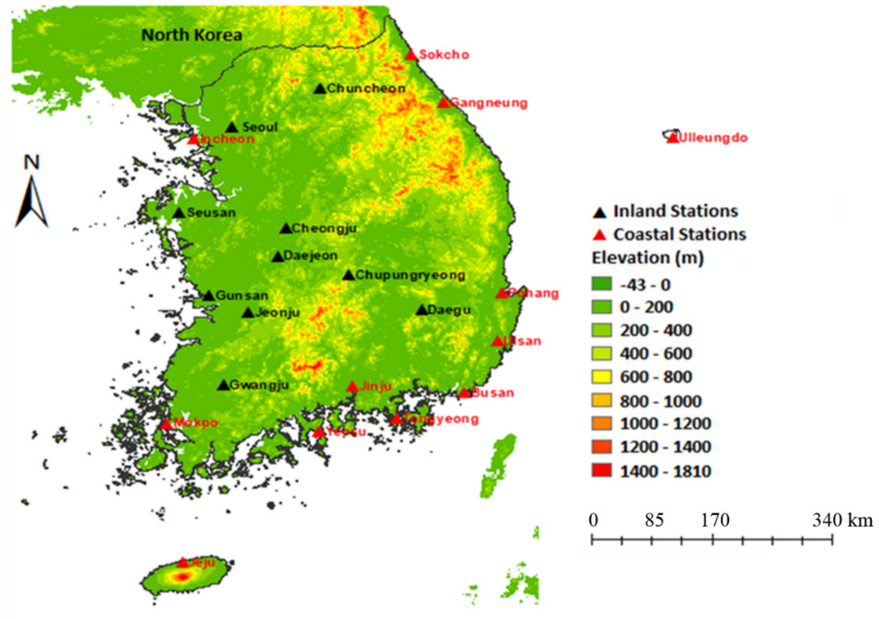
This study was conducted in South Korea (35°50′ N, 127°00′ W), which is located in East Asia between Japan and China. There is complex temporal and spatial variation in the climate of the country as it is strongly influenced by the East Asian monsoon and diverse topographical characteristics. There are four distinct seasons: winter (Dec–Feb), autumn (Sep–Nov), summer (Jun–Aug), and spring (Mar–May). The annual average precipitation across the country ranges from 1200 to 1500 mm with 60–70% of precipitation occurring in summer. The annual average temperature ranges from 10 to 15 °C. The country has a warm continental climate/humid continental climate in the Northwest to South Central regions, a humid subtropical climate in the South, and a warm oceanic climate in the East and part of the South. The elevation of the country ranges from −43 m in the West to 1810 m in the eastern and southern parts of the country (Figure 1).

2.2. Dataset and Sources

2.2.1. Observed Data

This study used observed data from the Korean Meteorological Agency (KMA). There are 96 gauge stations with historical data on precipitation in South Korea. However, the periods of data availability differ among stations. Stations with short availability (less than 30 years) are primarily located in the mountainous areas (Figure 1), and these stations are not considered in this study. This study used the observed data from 22 gauge stations over 35 years (1970–2005).

2.2.2. General Circulation Models

CMIP5 is a set of globally coordinated GCM simulations that comprise historical and future climate simulations assembled from different modeling groups. Following CMIP3, CMIP5 was significantly improved by including a greater number of GCMs and addressing several issues that were not considered in CMIP3 [9]. This study used the monthly historical and future precipitation data from 13 GCMs in the CMIP5 using the availability of RCPs 2.6, 4.5, 6.0, and 8.5 for South Korea. The names of the modeling centers, models, institutions, and resolutions are presented in

Table 1. Information on GCMs used in this study.

Modeling Centers	Models	Institutions	Resolution (Longitude × Latitude)
NSF-DOE-NCAR	CESM1-CAM5	National Science Foundation, Department of Energy, National Center for Atmospheric Research	1.25° × 0.94°
NCAR	CCSM4	National Center for Atmospheric Research	1.25° × 0.94°
CSIRO-QCCCE	CSIRO-Mk3.6.0	Commonwealth Scientific and Industrial Research Organisation in collaboration with the Queensland Climate Change Centre of Excellence	1.88° × 1.86°
BCC	BCC-CSM1.1	Beijing Climate Center, China Meteorological Administration	2.81° × 2.79°
	BCC CSM1.1(m)		1.13° × 1.12°
NOAAFGDL	GFDL-ESM2G	Geophysical Fluid Dynamics Laboratory	2.50° × 2.00°
	GFDL-ESM2M
GISS	GISS-E2-R	National Aeronautics and Space	1.88° × 1.86°
NIMR/KMA	HadGEM2-AO	National Institute of Meteorological Research/Korea Meteorological Administration	1.88° × 1.25
MRI	MRI-CGCM3	Meteorological Research Institute	1.13° × 1.12°
MIROC	MIROC5	Atmosphere and Ocean Research Institute National Institute for Environmental Studies (The University of Tokyo), and Japan Agency for Marine-Earth Science and Technology	1.41° × 1.40°
	MIROC-ESM	Japan Agency for Marine-Earth Science and Technology, Atmosphere and Ocean Research Institute (The University of Tokyo), and National Institute for Environmental Studies	2.81° × 2.79°
NCC	NorESM1-M	Norwegian Climate Centre	2.50° × 1.89°

.

3. Methodology

3.1. Procedure

The procedure used in this study was as follows:

• GCMs were selected from the pool of CMIP5 GCMs based on the availability of all RCPs for South Korea.
• All GCMs having all different resolutions were spatially downscaled to obtain the data of the 22 gauge stations using Inverse Distance Weighting (IDW).
• Bias corrections were made to the 13 GCMs using the observed precipitation data and 11 bias correction methods.
• The uncertainty of the 11 bias correction methods was quantified.
• The uncertainty of the 13 GCMs using the selected bias correction method was quantified.
• A robust bias correction method was selected using three evaluation metrics.
• The uncertainty of the four RCPs was quantified.
• The uncertainty of the nine 10-year time periods was quantified.
• The uncertainty of the locations by coastal and inland regions was quantified.

The five types of uncertainties were compared.

3.2. Bias Correction Methods

In this study, a total of 11 bias correction methods were used to correct biases in the GCMs. Of the 11 methods, nine used Quantile Mapping (QM); the other two used Deep Learning (DL) and Random Forest (RF) techniques.

3.2.1. Quantile Mapping

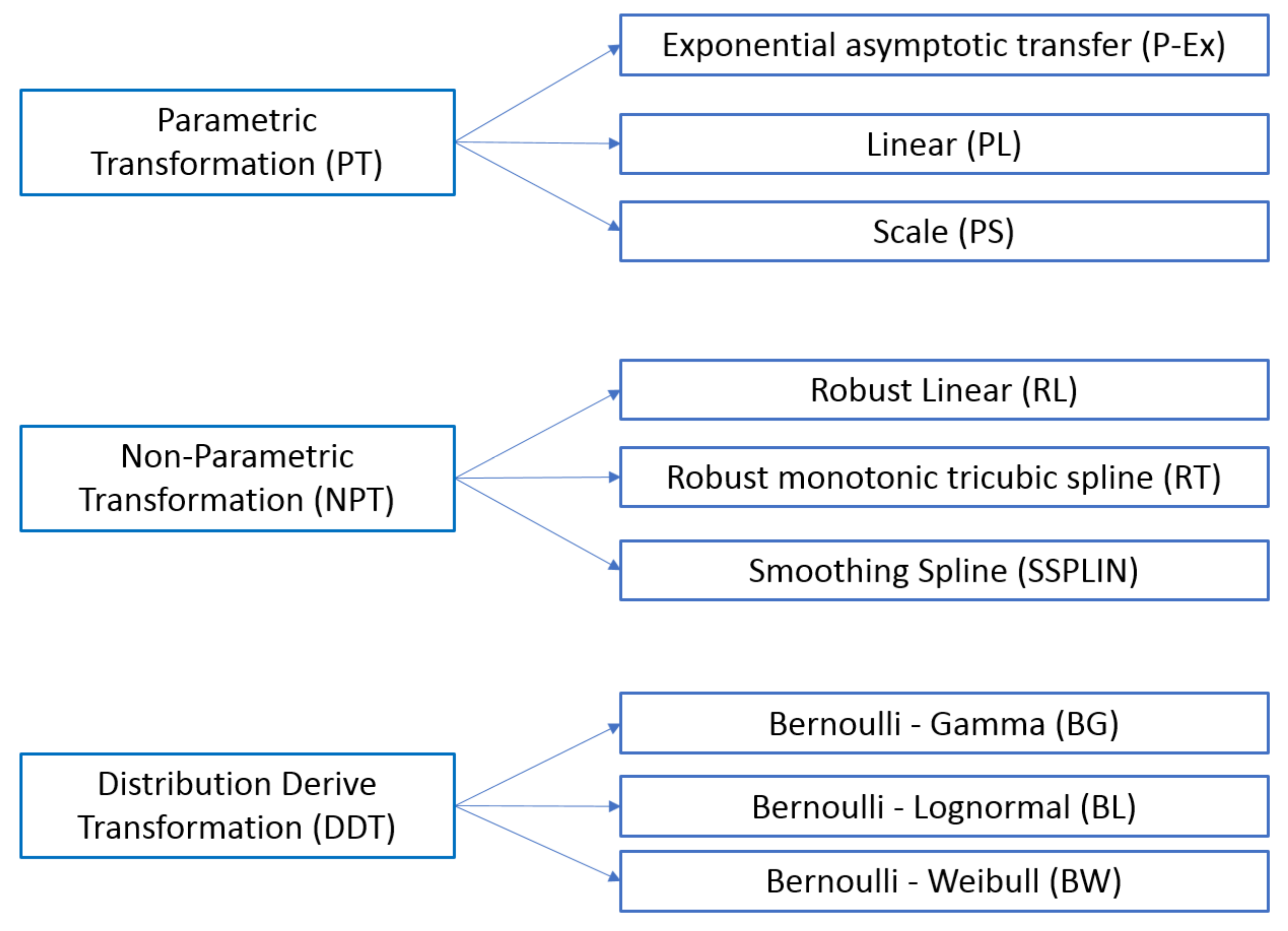
QM can be classified into Parametric Transformation (PT), Non-Parametric Transformation (NPT), and Distribution Derivation Transformation (DDT). The QM non-parametric technique [26] has the advantage of non-reliance on any predetermined statistical distribution of the data [27]. PT is a QM that has typically been used in the past [28]. QM builds a model variable (P_m) by using the probability integral transform in such a way that the newly constructed distribution becomes equal to the distribution of the observed variable (P_o).

$$P_o=h\left(P_m\right)$$

(1)

where $P_o$ is the observed precipitation value, $P_m$ is the simulated precipitation value of the GCM, and $h$ is the conversion function. Equation (2) is a distribution function based on Equation (1), and the observed precipitation value is calculated as the inverse of the cumulative distribution function (CDF).

$$P_o=P_o^{-1}\left(F_m\left(P_m\right)\right)$$

(2)

where $F_m$ is the CDF of $P_m$ and $P_o^{-1}$ is the inverse function of the CDF of $P_o$. There are three methods, which can be divided into exponential asymptotic transfer functions, (P-Ex), linear (PL), and scale (PS). The formulae for the three methods are presented as Equations (3)–(5).

$$P_o=\left(a+b\times P_m\right)\times \left(1-\exp \left(-\frac{P_m}{\tau }\right)\right)$$

(3)

$$P_o=a+bA\times P_m$$

(4)

$$P_o=bA\times P_m$$

(5)

where $P_o$ is the station precipitation value, $P_m$ is the simulated precipitation value of the GCM, $a$ is the additional correction coefficient, $b$ is the multiplicative correction coefficient, $\left(a+b\times P_m\right)$ is a formula for estimating the asymptote, and $\mathsf{\tau }$ is a value for determining a vector approaching the asymptote.

For NPT, Robust Linear (RL) and Smoothing Spline (SSPLIN) are frequently used [26,29,30]. Robust Linear regression is estimated using local linear least square regression to correspond to observed and simulation data in the quantile–quantile plot. SSPLIN is a method of estimation using the Smoothing Spline in quantile–quantile plot.

DDT involves the application of distribution functions in Equation (2). In this study, the Bernoulli–Gamma (BG), Bernoulli–Weibull (BW), and Bernoulli–Lognormal (BL) functions were used. Bernoulli was used to analyze the occurrence of a rainfall event, and Gamma, Weibull, and Lognormal were used to analyze precipitation distributions. The specific methods for QM used in this study are shown in Figure 2.

3.2.2. Random Forest

RF developed by Breiman [31] is one of the most successful machine (statistical) learning algorithms for practical applications. Despite its practical value, until very recently, and compared to other machine learning and artificial intelligence algorithms, random forests remained relatively obscure with limited use in water science and hydrological applications [32]. RF is a non-parametric statistical regression algorithm that produces numerous independent Classification and Regression Trees (CARTs). RF has superior performance for the tree decision-making process compared to the conventional method using hyperplane and it maximizes the advantages of ensemble theory. RF can be learned by calculating a simple hierarchical structure of complex and deterministic problems. This method automatically learns parameters from the learning data. RF has been identified as an effective and robust algorithm for bias correction in this study because: (1) the robustness of RF can avoid overfitting, (2) many different types of input variables can be implemented without variable deletion and regularization, and (3) it has analytical and operational flexibility.

3.2.3. Deep Learning

The Artificial Neural Network (ANN) proposed by McCulloch and Pitts [33] is a statistical algorithm that makes decisions patterned after the neural networks of human or animal brains. There are three components of ANNs: an input layer, several hidden layers, and an output layer. All layers are composed of various nodes, weights, and transition functions, and the optimal parameters and weights of the transition functions are determined in the learning phase. An ANN is mainly suitable for analyzing abnormal or nonlinear data. The ANN can be more accurate than the various statistical methods that are used if the amount of data that can be learned is secured, and it has great advantages in prediction and classification [34,35]. Also, ANN is used as a general-purpose approximator for sophisticated nonlinear regression [36]. Li and Zheng [37] derived that it is superior to conventional modeling methods regarding the ANN’s nonlinear system processing capability. Liu et al. [38] used it for global climate change and ecology studies. However, ANNs have a major problem of overfitting, which can be corrected to some extent by parameter adjustment. Hinton [39] used restricted Boltzmann machines to perform each layer’s pre-training to check the initialization point of Feedforward Neural Network (FNN) and solved the problem of overfitting by re-performing supervised backpropagation. This approach was applied in this study to avoid overfitting.

3.3. Inverse Distance Weighted Method

The Inverse Distance Weighted (IDW) method is a method typically used for studies that require geographical interpolation [40]. The IDW method is based on Tobler’s first law and is a method for interpolating the value of an unmeasured point; the value of the closest point is more relevant than a far point. In this study, Equation (6) was used to estimate the precipitation at the unmeasured point, and Equation (7) was used to estimate the weight.

$$P_i={\displaystyle \sum _{k=1}^N}\frac{w_s\left(x\right)}{{\sum }_{k=1}^N{w}_s\left(x\right)}{P}_i\left(x_s\right)$$

(6)

where $P_i$ represents the precipitation at the unmeasured point, and $P_i\left(x_s\right)$ represents the precipitation at the points surrounding the unmeasured point. In this study, the value of $P_i\left(x_s\right)$ was the GCM adjacent grid of unmeasured points, and the grid can use more than two points.

$$w_s\left(x\right)=\frac{1}{D_{\left(x,x_s\right)}^c}$$

(7)

where $w_s\left(x\right)$ is the interpolation weight and $D_{\left(x,x_s\right)}^c$ is the distance between the unmeasured and the measured points. The Lukaszk method and the Shepard method can both be used to calculate the weights. The Shepard method was used in this study. When the range of exponent c of $D^c$ is calculated to be a value between 0 and 1, the distribution of the data is narrowly interpolated, and when it is greater than 1, the distribution of the data is broadly interpolated. In this study, the value of c is set to 1 to consider only the effect of distance.

3.4. Evaluation Index

In this study, the performance of bias correction applied to GCM was compared. This study applied an excellent bias correction method in the forecast period and estimated the uncertainty of the period, RCP scenario, and location. Normalized Root Mean Square Error (NRMSE), Percent bias (Pbias), and Nash–Sutcliffe Efficiency (NSE) were used, and the above metrics are widely used to evaluate the results of the historical period of GCM [41]. NRMSE is shown in Equation (8). NRMSE removed the scale of RMSE, and the closer to 0, the higher the accuracy.

$$\mathrm{NRMSE}=\frac{\sqrt{\frac{1}{\mathrm{n}}{\sum }_{\mathrm{i}=1}^{\mathrm{n}}{\left({\mathrm{X}}_{\mathrm{s}}-{\mathrm{X}}_{\mathrm{o}}\right)}^2}}{\overline{{\mathrm{X}}_{\mathrm{o}}}}$$

(8)

Pbias is shown in Equation (9), and it is an indicator of bias. The tendency for the simulated value of GCM to be overestimated is calculated as a positive Pbias, and the closer to 0, the optimal value.

$$\mathrm{Pbias}=\frac{{\sum }_{\mathrm{i}=1}^{\mathrm{n}}\left({\mathrm{X}}_{\mathrm{o}}-{\mathrm{X}}_{\mathrm{s}}\right)}{{\sum }_{\mathrm{i}=1}^{\mathrm{n}}{\mathrm{X}}_{\mathrm{o}}}$$

(9)

NSE is shown in Equation (10). It is used to verify the accuracy of observed and GCM precipitation in water research. The negative value indicates that the correlation between GCM and observed precipitation is low, and the performance is low. The positive value means a high correlation and high performance.

$$\mathrm{NSE}=1-\frac{{\sum }_{\mathrm{i}=1}^{\mathrm{n}}{\left({\mathrm{X}}_{\mathrm{s}}-{\mathrm{X}}_{\mathrm{o}}\right)}^2}{{\sum }_{\mathrm{i}=1}^{\mathrm{n}}{\left({\mathrm{X}}_{\mathrm{o}}-\overline{{\mathrm{X}}_{\mathrm{o}}}\right)}^2}$$

(10)

In Equations (8)–(10), ${\mathrm{X}}_{\mathrm{s}}$ is the simulated value of GCM, and ${\mathrm{X}}_{\mathrm{o}}$ is the observed value. $\overline{{\mathrm{X}}_{\mathrm{o}}}$ means the average of the observed data.

4. Results

In this study, the uncertainties in historical and projected rainfall arising from five sources were analyzed. Uncertainty sources considered in this study included: (1) bias correction methods, (2) GCMs, (3) RCPs, (4) future periods, and (5) locations within the study area. The results obtained are presented in the corresponding sections. In each sub-section, there are many results for 22 stations. Due to the space limitation, the result for a representative station that showed the general characteristics is shown for Seoul in Section 4.1, Section 4.2, Section 4.4, Section 4.5 and Section 4.6 and Busan in Section 4.3.

4.1. Uncertainty in Bias Correction Methods

4.1.1. Historical Period

The Probability Density Functions (PDFs) of the monthly precipitation for the 13 GCMs for all bias correction methods at the Seoul station are shown in Supplementary Materials Figure S1. The PDFs from some bias correction methods were very similar to the observed data, whereas other methods overestimated or underestimated rainfall in some GCMs. The average monthly precipitation obtained from 11 bias correction methods for the Seoul station for the different GCMs is shown in Supplementary Materials Figure S2. The average monthly precipitation varied from 100.3 mm for BW to 159.8 mm for DL, and the range of the averages of the GCMs spanned from 3.1 mm for BG to 21.3 mm for BC and BW. The differences among the bias correction methods were not large except for several methods.

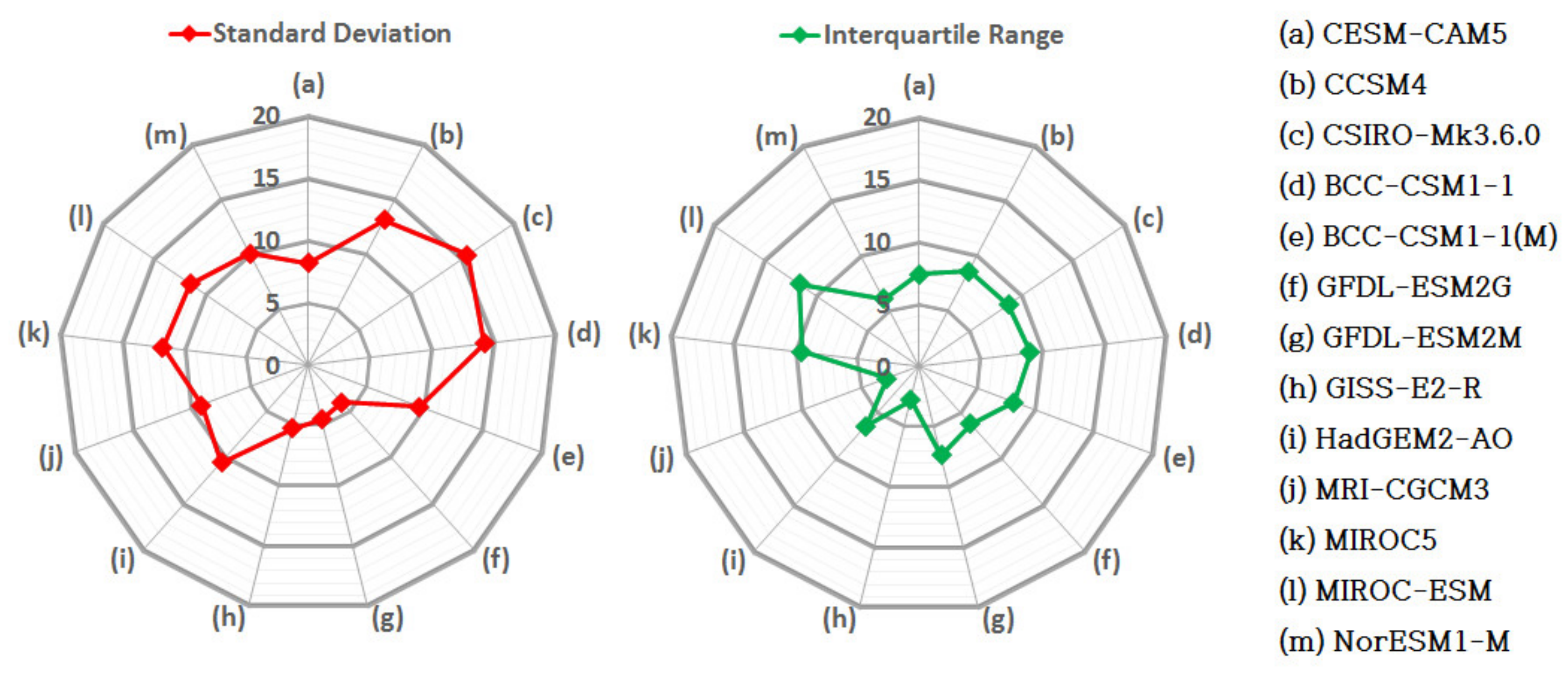
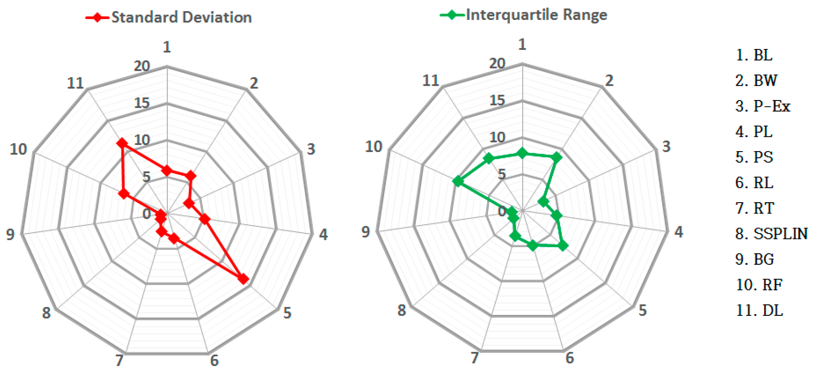
To quantify the uncertainty, the STDEVs and IQRs for the average monthly precipitation from the 11 bias correction methods were calculated for each GCM, and the results are presented in Figure 3. The maximum STDEV was 11.7 mm for MIROC-ESM, and the minimum was 4.0 mm for GFDL-ESM2G. A median STDEV of 10.1 mm was observed for NorESM1-M. The maximum value of the IQR was 11.6 mm for MIROC-ESM, and the minimum value was 2.8 mm for MRI-CGCM3 and GISS-E2-R. The median IQR was 7.4 mm for all GCMs. This indicates that MIROC-ESM was characterized by the highest uncertainty compared with the other GCMs.

4.1.2. Future Projection Period

The PDFs of bias-corrected precipitation for all GCMs during the period 2011–2100 are shown in Supplementary Materials Figure S3. The average monthly precipitation obtained from the 11 bias correction methods for the Seoul station was calculated for all GCMs and is shown in Supplementary Materials Figure S4. The averages ranged from 86.8 mm for RF to 184.7 mm for BL and BW in all GCMs and the range of the averages of the GCMs spanned from 29.6 mm for SSPLIN to 88.0 mm for BW. Accordingly, the values for the future projections were higher and their range was broader than those for the historical period.

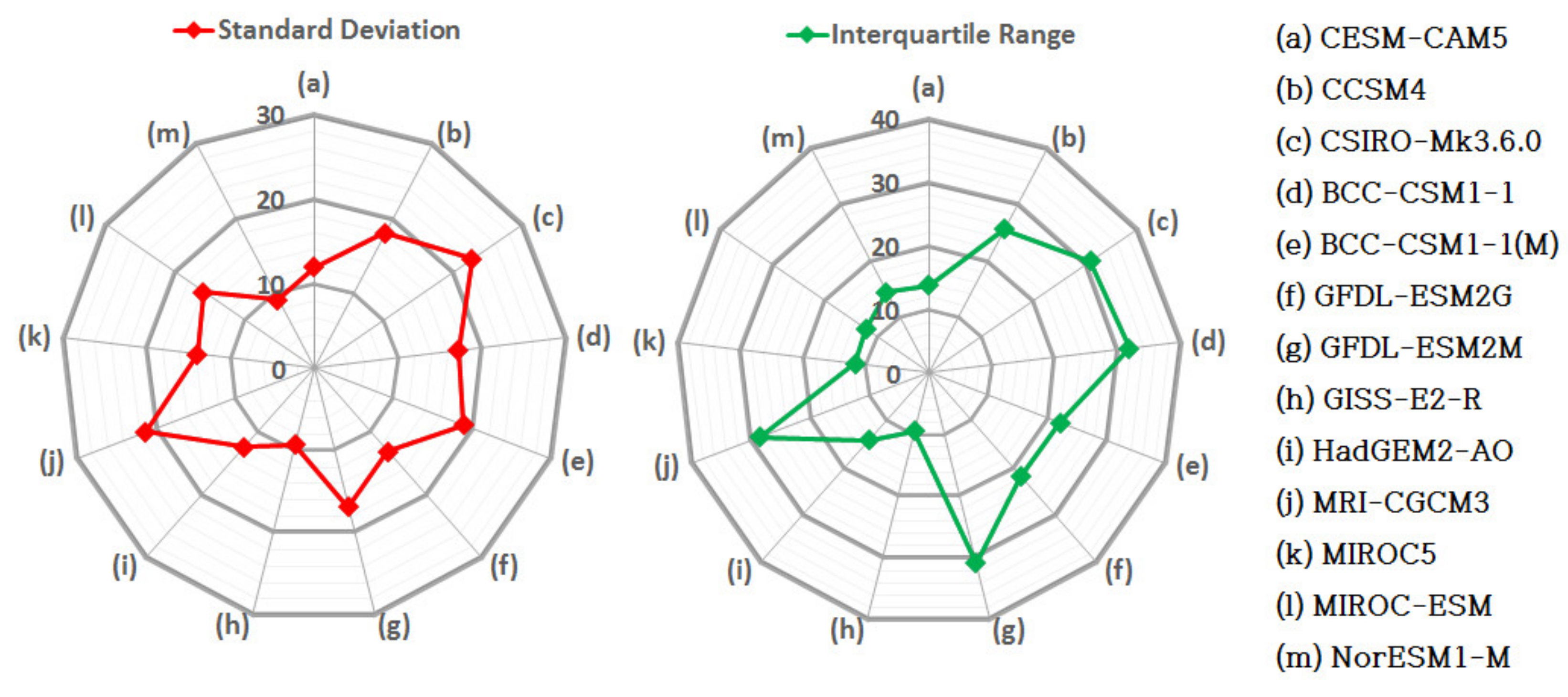
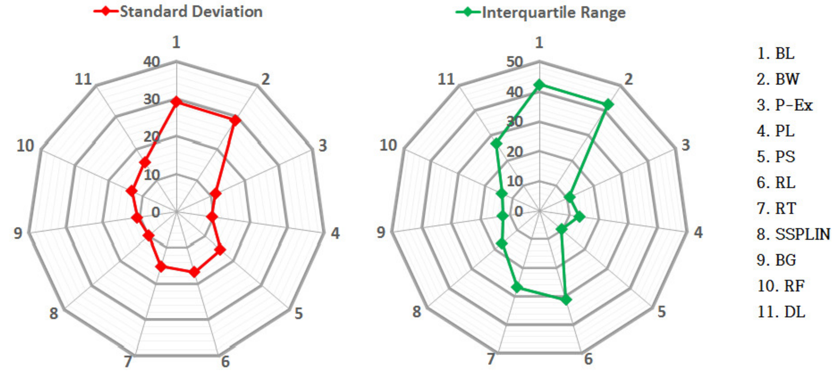
To quantify the uncertainty, the STDEVs and IQRs for the average monthly precipitation from the 11 bias correction methods were calculated for each GCM and the results are shown in Figure 4. The maximum STDEV was 21.5 mm for CSIRO-Mk3.6.0, and the minimum was 8.6 mm for NorESM1-M. The median STDEV was 16.4 mm for GFDL-ESM2M. The STDEVs for the projection period were much higher than those for the historical period. This finding indicates that there is a broader distribution of average monthly precipitation for the projection period in most GCMs.

The maximum value of the IQR was 29.7 mm for GFDL-ESM2M, and the minimum value was 10.1 mm for NorESM1-M. The median IQR was 24.4 mm for GFDL-ESM2G. Similar to the STDEV, these three IQRs were higher than those of the historical period. This finding indicates higher uncertainty in projected precipitation compared to the historical period.

4.2. Uncertainty in GCMs

4.2.1. Historical Period

The PDFs for the bias-corrected precipitation of the 13 GCMs and the observed precipitation using the different bias correction methods are shown in Supplementary Materials Figure S5. The precipitation distributions are similar for most of the GCMs and most of the bias correction methods. The greatest variation in the distribution of precipitations was in CESM1-CAM5 and CCSM4 using the PS bias correction method. Other GCMs such as CSIRO-Mk3.6.0 and GISS-E2-R were not able to replicate the properties of the observed data from the PDF. MIROC5 and HadGEM-2-AO were best able to replicate the observed precipitation distribution.

The average monthly precipitation of bias-corrected GCMs for the Seoul station was calculated using the 11 bias correction methods and is shown in Supplementary Materials Figure S6. The maximum average monthly precipitation of 153.8 mm was calculated for BCC-CSM1-1, and a minimum of 100.3 mm was calculated for CSIRO- Mk3.6.0. The range of the averages of bias-corrected precipitation based on the bias correction methods spanned from 11.8 mm for GFDL-ESM2G to 47.4 mm for CCSM4.

The STDEVs and IQRs of the average monthly precipitation from the 13 GCMs for the historical period were calculated for each bias correction method and are presented in Figure 5. The highest STDEV was 16.4 mm for DL, indicating the highest level of uncertainty among the methods. The minimum value was 0.9 mm for BG, indicating a lower level of uncertainty and similar precipitation results regardless of the type of GCM. The results of the IQRs were very similar to those of the STDEVs. The largest IQR was obtained from DL and the smallest was obtained from BG.

4.2.2. Future Projection Period

The PDFs of the bias-corrected precipitation of the 13 GCMs for the projection period from the different bias correction methods are presented in Supplementary Materials Figure S7. The PDFs of the GCMs were similar for many of the bias correction methods. The most dissimilar GCM was CCSM4, as seen from the PDFs of BL, BW, BG, and RF. The greatest variability in the distribution of precipitation in the GCMs was for the PS bias correction method. The average monthly precipitation of bias-corrected GCMs for the Seoul station was calculated for the 11 bias correction methods and is shown in Supplementary Materials Figure S8. The maximum average monthly precipitation was 184.7 mm for MIROC-ESM, and the minimum was 86.8 mm for BCC-CSM1-1. The range of the averages of the bias correction methods spanned from 24.9 mm for NorESM1-M to 69.5 mm for CSIRO-Mk3.6.0. These values are higher, and their ranges are broader than those for the historical period.

The STDEVs and IQRs of the average monthly average precipitation from the 13 GCMs for the projection period were calculated for each bias correction method and are presented in Figure 6. The highest STDEVs were observed in BL (29.0 mm) and BW, indicating the greatest uncertainty among these methods. The lowest STDEVs were observed for PL (9.5 mm), indicating a lower level of uncertainty, which is consistent with similar projections regardless of the type of GCM. In addition, the largest IQRs were again found in BL and BW (42.2 mm), and the smallest were calculated for P-Ex (10.9 mm) and PS (9.6 mm). The STDEVs and IQRs from all GCMs were higher than those for the historical period.

4.3. Selection of Bias Correction Method

To quantify the uncertainties based on the RCPs, the projection period, and the locations, a robust high-performing bias correction method should be consistently used for all GCMs. Therefore, the robust bias correction method should be selected based on various performances.

The 11 bias correction methods used in this study were analyzed using three evaluation indicators: Pbias, NSE, and NRMSE. NRMSE and Pbias values closer to 0 indicate better performance, whereas, NSE values closer to 1 indicate better performance. Standardization was performed based on the three estimated evaluation indicators; if the standardized performance was closer to 1, the performance had improved, and if it was closer to 0, the performance had deteriorated. To determine the final performance for each bias correction method at each station for each GCM, the average of the performance indicators for the individual station was taken. As a representative example, the performances of the different bias correction methods for the Busan station are presented by GCMs in

Table 2. Standardized statistical metrics for evaluation of bias correction methods for each GCM at Busan station.

Name of GCM	DL	BL	BW	P-Ex	BG	PL	RF	RL	RT	PS	SSPLIN
CAM	0.903	0.619	0	0.924	0.964	0.708	0.544	0.990	0.999	0.924	0.81
CCSM4	0.928	0	0.541	0.953	0.970	0.888	0.758	0.927	0.947	0.953	0.833
CSIRO	0.962	0.026	0.549	0.985	0.938	0.956	0.793	0.949	0.984	0.985	0.89
CSM1.1	0.874	0.923	0.356	1	0.983	0.872	0.32	0.912	0.92	1	0.923
CSM1.1M	0.986	0.375	0	0.97	0.988	0.773	0.519	0.986	0.996	0.97	0.877
ESM2G	0.958	0	0.882	0.987	0.99	0.993	0.673	0.988	0.998	0.987	0.952
ESM2M	0.899	0	0.937	0.945	0.982	0.977	0.636	0.991	0.991	0.945	0.988
GISS	0.854	0.214	0.457	0.891	0.936	0.888	0	0.91	0.929	0.891	0.989
HADAO	0.881	0.104	0.162	0.978	0.979	0.843	0.583	0.973	0.98	0.978	0.992
MIROC5	0.82	0.769	0	0.986	0.961	0.764	0.329	0.971	0.991	0.986	0.94
MIROCESM	0.926	0.53	0	0.99	0.987	0.802	0.522	0.986	0.992	0.99	0.893
MRI	0.854	0.614	0	0.941	0.969	0.727	0.391	0.969	0.988	0.941	0.950
NOR	0.898	0.932	0.351	1	0.979	0.875	0.313	0.988	0.986	1	0.927
Average	0.903	0.393	0.326	0.965	0.971	0.851	0.491	0.965	0.977	0.965	0.920

because the individual values of Busan station are relatively similar to the averages of all stations. The results of the Seoul station representing the main area in Korea are also shown in Supplementary Materials Table S1. This table also shows the average of the scores for each of the methods from the different GCMs. RT had the best performance for most GCMs followed by BG, P-Ex, RL, and PS. GISS and HADAO had the best performances using the SSPLIN method. BW, BL, and RF exhibited the poorest performances. Therefore, careful selection of the bias correction method is necessary because the performances of all GCMs in the reproduction of historical climate were substantially different.

The ranking of the performances for the 11 bias correction methods was derived from the observed data from the 22 stations in South Korea, as shown in

Table 3. The number of times showing the best performance by each bias correction method.

Name of GCM	DL	BL	BW	P-Ex	BG	PL	RF	RL	RT	PS	SSPLIN
CAM	1	0	0	0	1	0	0	4	4	0	12
CCSM4	0	0	0	0	7	0	0	1	1	0	13
CSIRO	0	0	0	3	0	0	0	2	6	4	11
CSM1.1	1	0	0	5	1	0	0	2	3	4	10
CSM1.1M	0	1	0	0	2	0	0	2	3	0	14
GFDL-ESM2G	0	0	0	1	2	1	0	4	2	1	12
GFDL-ESM2M	0	0	0	0	1	2	0	3	2	0	14
GISS	1	0	0	1	0	0	0	3	3	1	14
HADAO	1	0	0	2	0	0	0	2	3	2	14
MIROC5	0	0	0	3	1	0	0	2	1	2	15
MIROCESM	0	0	0	0	1	0	0	2	3	0	16
MRI	0	0	0	0	3	0	0	1	3	0	15
NOR	0	0	0	4	0	0	0	2	4	4	12
Overall	4	1	0	19	19	3	0	30	38	18	172

. This table shows the number of stations where each bias correction method was selected as having the best performance. Overall, the SSPLIN method exhibited the best performance. SSPLIN was selected 172 times, which represents 60.1% of all cases (286 = 13 GCM × 22 stations). The rank of the remaining methods was as follows: RT (38 times, 13.3%), RL (30 times, 10.5%), BG (19 times, 6.6%), and P-Ex (19 times, 6.6%), followed by relatively low frequencies of top ranking for DL (4 times), PL (4 times), and BL (1 time).

4.4. Uncertainties in the RCP Scenario

The results of the uncertainties based on the RCP scenarios are discussed in this section for the SSPLIN method, which had the best performance among all bias correction methods. The PDFs of all GCM simulations for the four RCPs are presented in Supplementary Materials Figure S9. The PDFs were similar for the RCPs of the different GCMs. However, RCP 8.5 showed a different distribution of precipitation for BCC-CSM1-1(M).

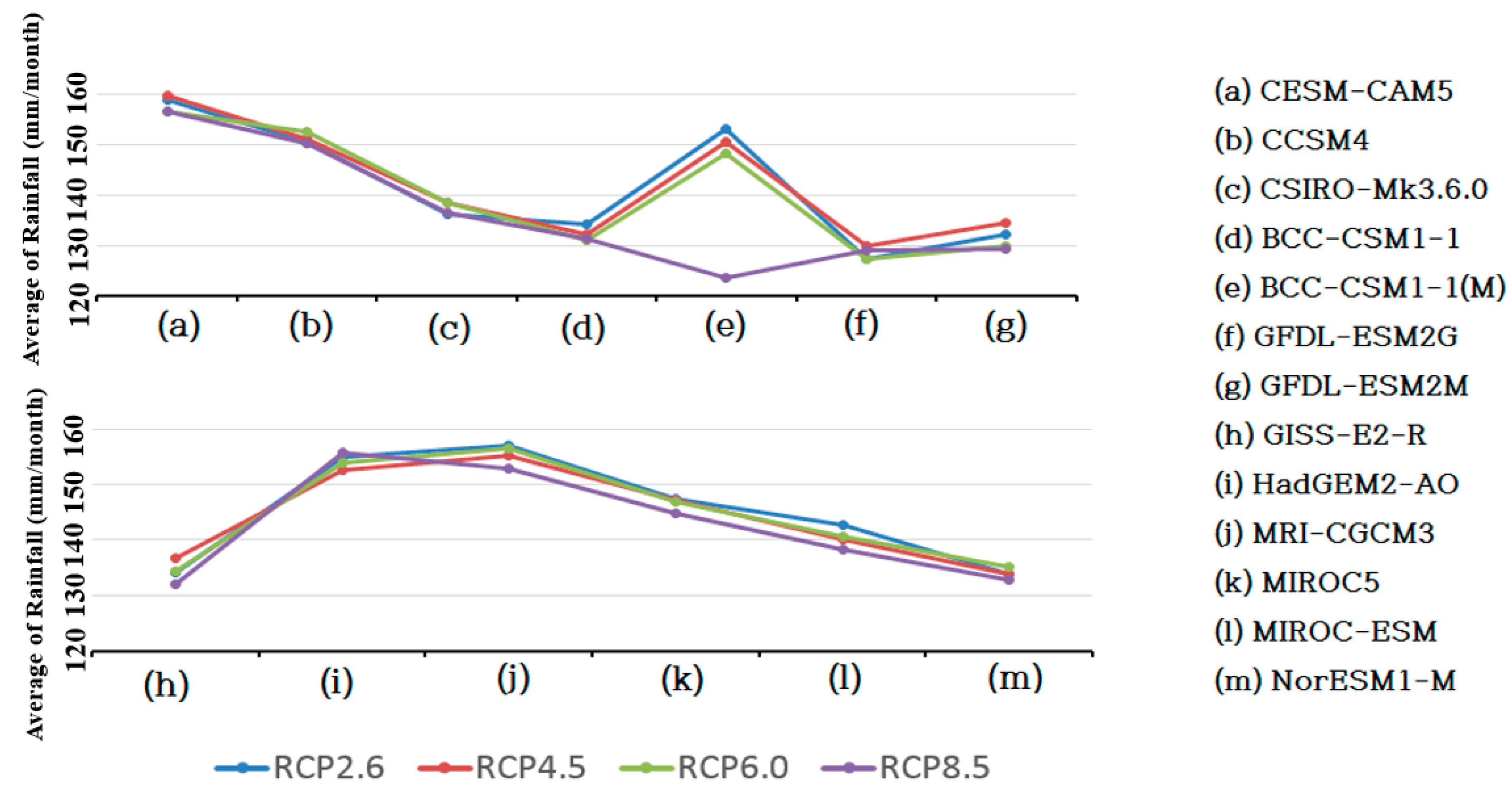
The average monthly precipitation for the four RCPs is presented for all GCMs in Figure 7. The ranges of the average precipitation for RCP 2.6, 4.5, 6.0, and 8.5 were 127.6–158.9 mm, 130.0–159.0 mm, 127.4–156.5 mm, and 123.6–156.5 mm, respectively. RCP 8.5 had the largest range (32.9 mm) followed by RCP 2.6 (31.3 mm), RCP 4.5 (29.6 mm), and RCP 6.0 (29.2 mm). There was little variation among the RCPs except for BCC-CSM1-1M, which had a much lower average monthly precipitation for RCP 8.5. CESM-CAM5 had the maximum average monthly precipitation of all RCPs, and GFDL-ESM2M had the minimum average monthly precipitation for RCPs 2.6, 4.5, and 6.0. The differences among the RCPs were 2.2–5.2 mm for all GCMs except for BCC-CSM1-1(M), which was 29.5 mm, as shown in Figure 7.

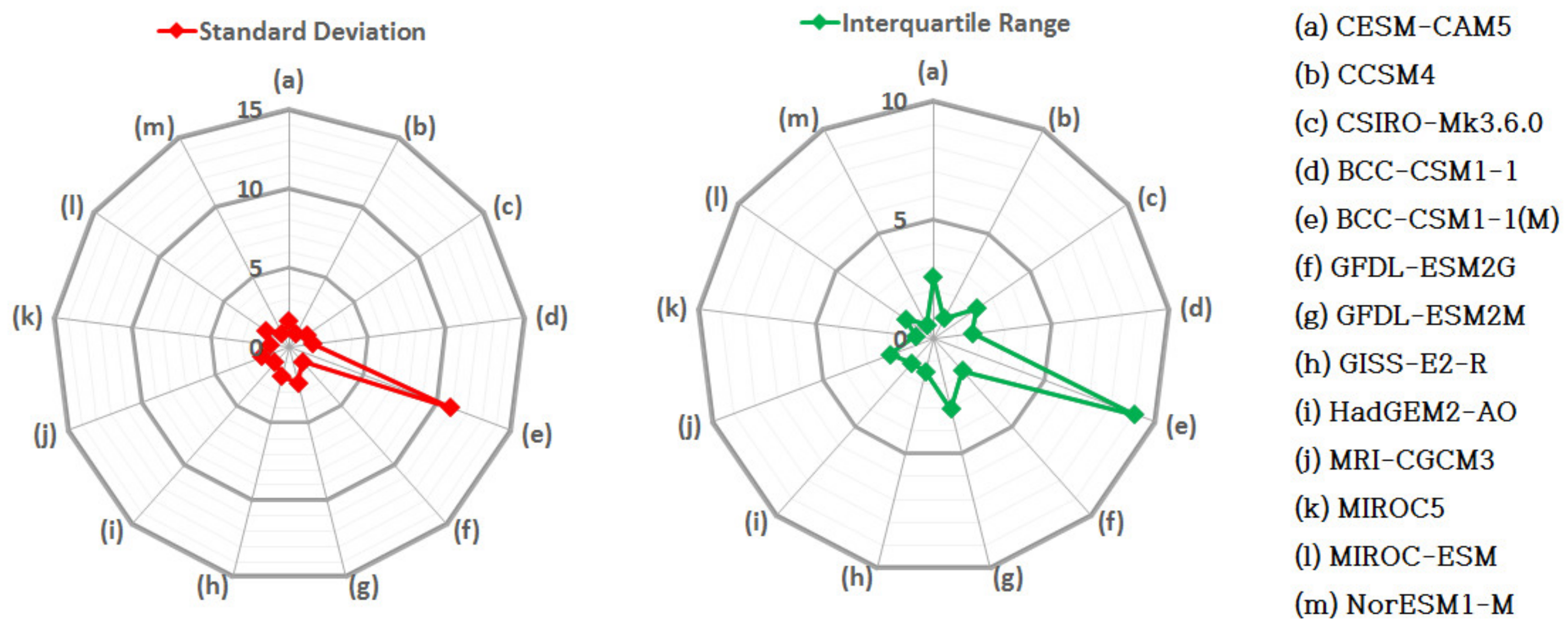
The STDEVs and IQRs for the four RCPs for the different GCMs are presented in Figure 8. The maximum STDEV was 10.9 mm, which was calculated for BCC-CSM1-1(M). However, most STDEVs, except for BCC-CSM1-1(M), were low; the median STDEV was 1.5 mm. The minimum STDEV was 0.95 mm for CCSM4. The maximum IQR was 9.05 mm, which was also calculated for BCC-CSM1-1(M). As with the STDEVs, the IQRs were also low for all GCMs, except for BCC-CSM1-1(M). The minimum IQR was 0.61 mm for NorESM1-M.

4.5. Uncertainties in Projection Periods

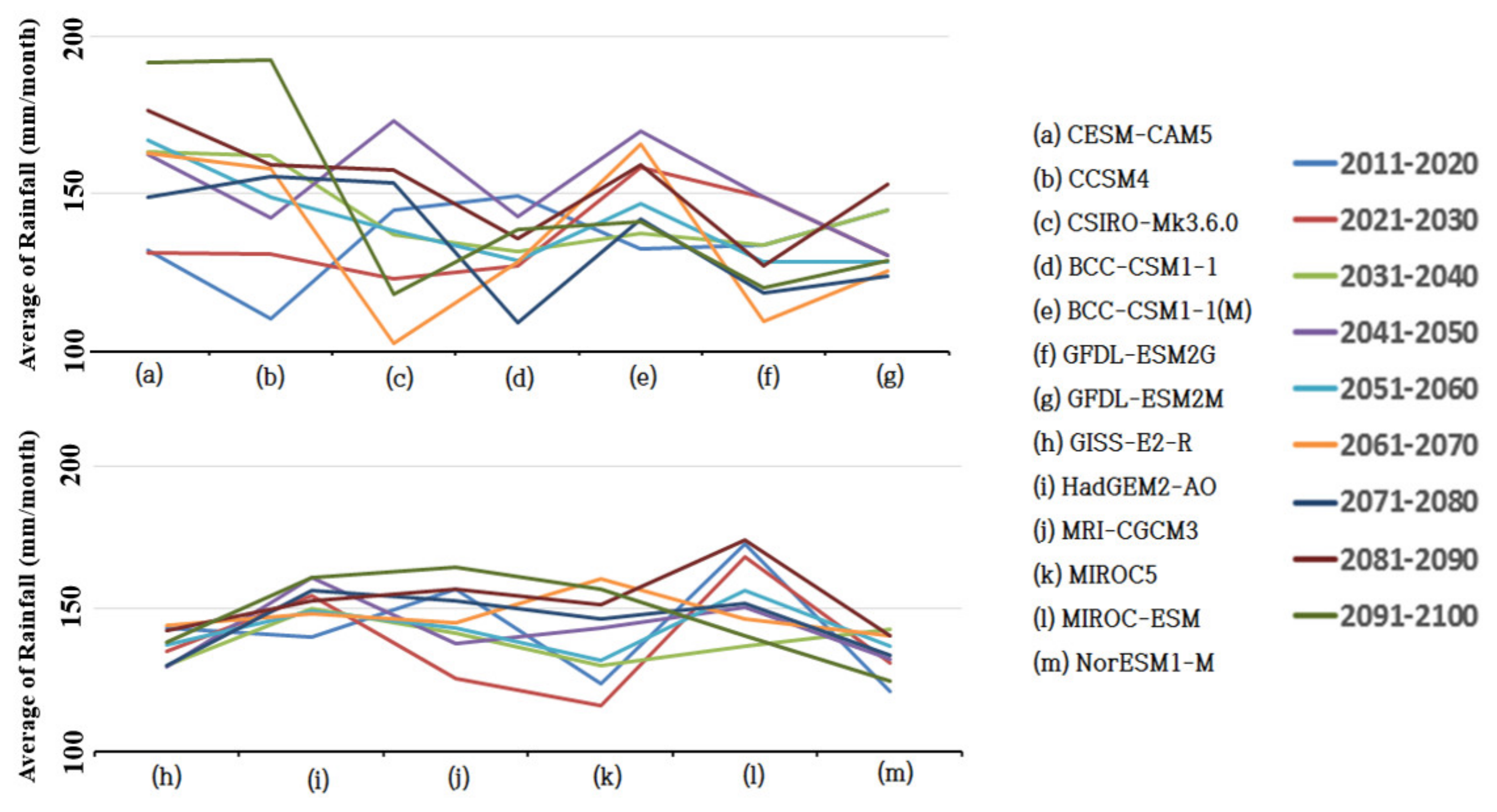
This section presents the results of the downscaling using the SSPLIN method for RCP 4.5 for the Seoul station over 10-year intervals from 2011 to 2100. The monthly precipitation for the nine 10-year periods for all GCMs at the Seoul station is shown in Figure 9. The ranges of precipitation were 110.5–172.7 mm for 2011–2020, 130.3–163.4 mm for 2031–2040, 128.5–167.1 mm for 2051–2060, 109.1–156.6 mm for 2071–2080, and 118.2–192.4 mm for 2091–2100 for all GCMs as shown in Supplementary Materials Figure S10. These data indicate that there will be variation in the average monthly precipitation during different periods of the century.

Figure 9 shows the monthly average precipitation at Seoul station divided into nine periods for the projection period of RCP4.5 in 13 GCMs. The widest range of average monthly precipitation for these periods was observed for CCSM4 with a range of 110.5–192.4 mm, and the smallest range was observed for GISS-E2-R with a range of 129.7–144.4 mm. The narrowest range of average monthly precipitation was for HadGEM2-AO and NorESM1-M with 140.1–161.1 mm and 121.0–143.1 mm of precipitation, respectively. As a result, all GCMs have their own decadal variations which are largely different from each other.

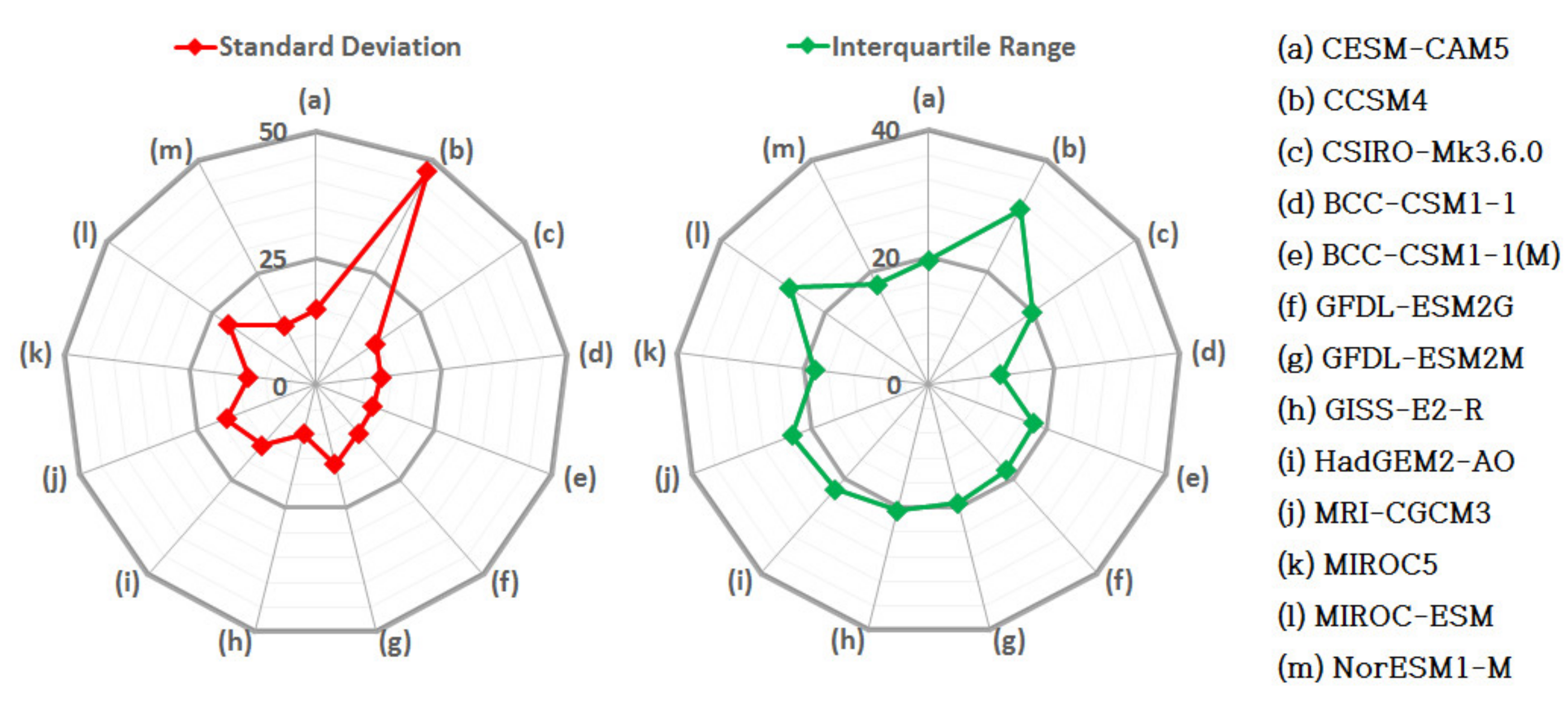
The STDEVs and IQRs of the GCM simulations for the nine time periods are shown in Figure 10. The maximum STDEV was 14.8 mm for CCSM4, and the minimum STDEV was 3.2 mm for GISS-E2-R. The range was 11.6 mm. CESM-CAM5 and CCSM4 showed high STDEVs, indicating that they have greater variation over time. The GCMs with the largest IQRs were the same as those for the STDEVs. However, the second and third largest GCMs were GFDL-ESM2G and MIROC5, and the third smallest was MIROC-ESM.

4.6. Uncertainty by Location

To analyze the uncertainties in projected precipitation based on location, the stations within the study area were classified as coastal or inland areas, as the meteorological characteristics of the two regions differed. The results are presented for the SSPLIN bias correction method for RCP 4.5.

4.6.1. Coastal Areas

The PDFs of the bias-corrected precipitation for the coastal stations are presented in Supplementary Materials Figure S11. There was a wide range of PDFs among the coastal stations as observed from the width of the PDFs. The maximum monthly precipitation varied from 286.8 mm at Ulleungdo to 1023.9 mm at Pohang. The range of the maximum monthly precipitation for the coastal area was 737.1 mm. This wide range in precipitation can be attributed to Pohang being closer to the equator (latitude 36.03) than Ulleungdo (latitude 37.48). Pohang is more strongly influenced by equatorial factors. The distribution of precipitation showed that the lower the latitude of a station, the higher the monthly precipitation. Higher monthly precipitation is expected at the stations located in the southeastern coastal areas.

The bias-corrected average monthly precipitation for the 12 coastal regions was calculated for all GCMs and is presented in Supplementary Materials Figure S12. The average monthly precipitation varied from 85.1 to 287.5 mm across all coastal regions. However, these two extreme cases both occurred at Pohang. Similarly, the values for Ulsan were 100.2–195.3 mm. Precipitation was expected to be high for CCSM4 at the Pohang and Ulsan stations.

The STDEVs and IQRs for the 12 gauge stations are presented by GCM in Figure 11. The highest STDEV was 47.3 mm for CCSM4, indicating the greatest uncertainty of the locations. In contrast, the lowest STDEV was 10.0 mm for GISS-E2-R and thus the range was 37.3 mm. Similar to the STDEV results, the IQRs were largest (31.0 mm) for CCSM4 and smallest (11.4 mm) for BCC-CSM1-1.

4.6.2. Inland Areas

The PDFs of the bias-corrected precipitation for the inland stations are shown in Supplementary Materials Figure S13. The maximum monthly precipitation of the PDFs varied from 312.5 mm for Daegu to 789.6 mm for Daejeon. The range of precipitation was 477.1 mm, which is much smaller than that for the coastal areas by 260.1 mm. Although the maximum precipitation for the inland areas was lower than that for the coastal areas, the PDFs of precipitation at the inland stations were broader and the precipitation was more widely distributed. In addition, the shapes of the PDFs in the inland areas were relatively similar to one another, compared to those of the coastal areas. However, some inland areas such as Busan and Ulsan showed variability in the distribution of precipitation for some GCMs such as CCSM4, CSIRO-Mk3.6.0, BCC-CSM1-1, GFDL-ESM2G, and HadGEM2-AO.

The bias-corrected average monthly precipitation for the 10 inland stations was calculated for all GCMs and is shown in Supplementary Materials Figure S14. The maximum average was 184.9 mm at Chuncheon, and the minimum average was 86.5 mm at Deagu.

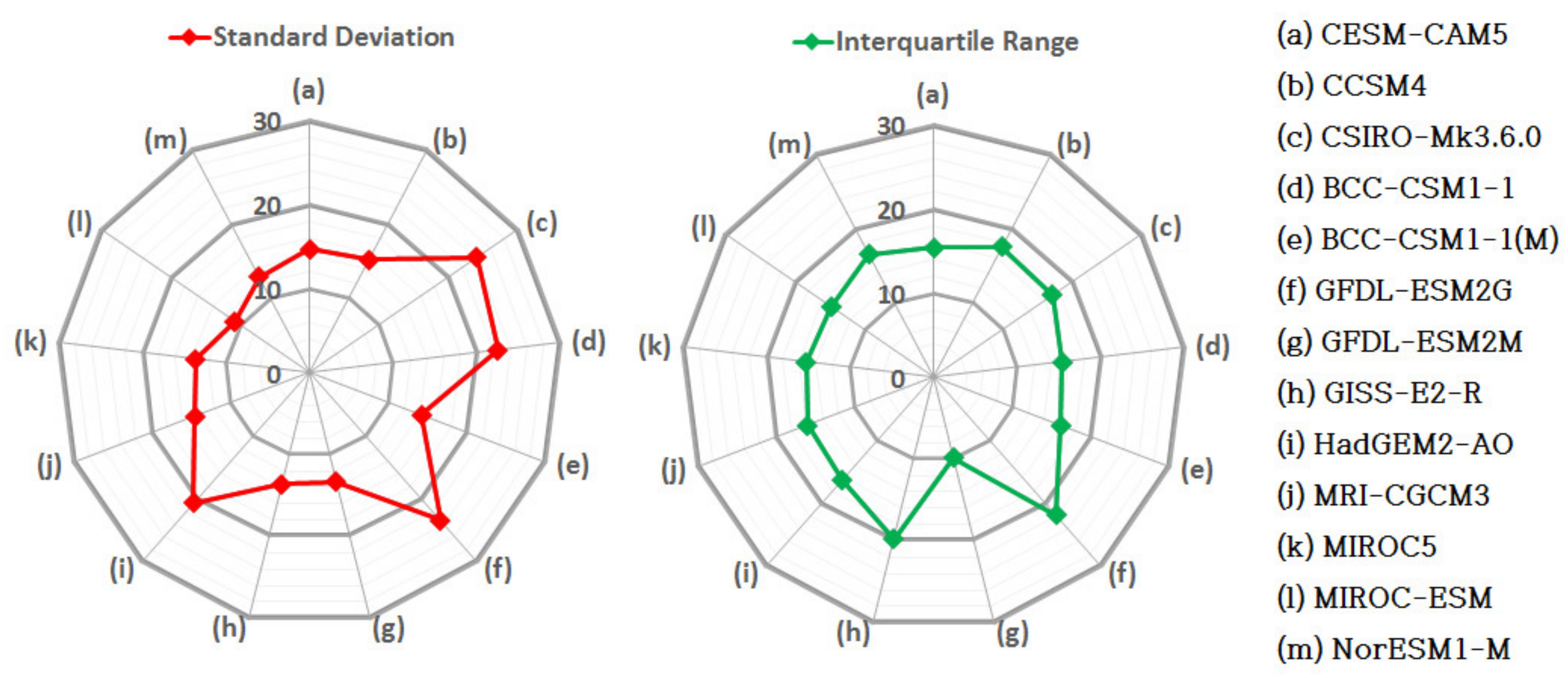
The STDEVs and IQRs for the 10 weather stations are presented by GCM in Figure 12. The STDEVs from the inland stations are lower than those from the coastal stations. The maximum STDEV was 24.1 mm for CSIRO-Mk3.6.0, and the minimum was 10.7 mm for MIROC-ESM. The range of the STDEVs was 13.4 mm. The next highest STDEVs were observed for GFDL-ESM2G, BCC-CSM1-1, and HadGEM2-AO with 23.4, 22.5, and 20.7 mm, respectively.

The IQRs for the inland areas were also lower than those for the coastal areas, indicating less uncertainty. The maximum IQR was 21.9 mm for GFDL-ESM2G, and the minimum IQR was 9.9 mm for GFDL-ESM2M. The range was 12.0 mm, which is smaller than that for the coastal area.

5. Discussion

The summary of STDEV and IQR analyses for the historical and projection periods is shown in

Table 4. STDEV and IQR analysis results for the historical period and projection period by GCMs.

Name of GCM	Historical Period		Projection Period
	Bias Correction		Bias Correction		RCPs		Period		Location
									Coastal		Inland
	STDEV	IQR	STDEV	IQR	STDEV	IQR	STDEV	IQR	STDEV	IQR	STDEV	IQR
CAM	8.1	7.3	11.9	13.8	1.6	2.6	19.6	18.3	14.8	19.4	14.7	15.4
CCSM4	13.1	8.6	18.0	25.5	1.0	0.9	22.7	16.6	47.3	31.0	15.1	17.5
CSIRO	15.4	8.7	22.7	30.9	1.3	2.2	21.7	30.5	14.3	19.8	24.1	17.2
CSM1.1	14.2	8.9	17.1	31.8	1.5	1.6	11.5	10.4	13.0	11.4	22.5	15.3
CSM1.1M	9.5	8.1	18.9	22.1	10.9	9.1	13.4	18.2	12.0	17.7	14.2	16.1
GFDL-ESM2G	4.0	6.2	13.1	21.8	1.2	1.8	13.3	13.7	12.7	18.2	23.4	21.9
GFDL-ESM2M	4.5	7.4	16.9	30.8	2.4	3.1	10.3	16.3	16.1	19.4	13.3	9.9
GISS	5.2	2.8	9.2	9.4	1.9	1.4	5.8	12	10.0	20.5	13.6	19.8
HADAO	10.4	6.4	12.4	14.1	1.4	1.4	6.7	7.6	15.8	22.2	20.7	16.3
MIROC5	9.1	2.8	21.2	28.4	1.8	1.9	11.9	15.3	18.7	23.0	14.5	16.0
MIROCESM	11.7	9.5	13.9	11.6	1.2	0.8	15.2	21	13.2	18.1	13.5	15.2
MRI	11.4	11.6	15.8	12.0	1.8	1.4	13.6	22	20.7	26.6	10.7	14.7
NOR	10.1	6.1	9.2	14.3	1.0	0.6	7.4	9.3	13.1	17.6	12.8	16.5
Overall	9.8	7.3	15.4	20.5	2.2	2.2	13.3	16.2	17.1	20.4	16.4	16.3

. For the historical period, the STDEVs and IQRs of the precipitation based on the type of bias correction method were higher than those based on the type of GCM. In contrast, for the projection period, the uncertainties related to the different bias correction methods were smaller than those related to the different GCMs.

The least uncertainty was observed among the four RCP scenarios, with a 2.2 mm STDEV and IQR. The next lowest level of uncertainty was related to the time period, with a STDEV and IQR of 13.3 and 16.2 mm, respectively. Therefore, the selection of the target future time period is much more important than the target RCP scenario.

The STDEVs and IQRs of the bias-corrected precipitation for the GCMs for the coastal and inland locations were compared. The results indicated that there was less uncertainty in the projected precipitation of the inland stations compared to that of the coastal stations.

Overall, the uncertainties based on bias correction methods, GCMs, and location all showed a similar magnitude, which was larger than the other sources of uncertainty. However, it can be concluded that the uncertainty in inland areas is lower than those from the other three sources, and the uncertainty in the GCMs are slightly higher than those from the bias correction methods during the projection period. In other words, the uncertainty in the projected precipitation in the coastal areas may be the intermediate between that of the bias correction methods and the GCMs for some criteria, or, overall, the largest among all kinds of uncertainty considered in this study (see Table 4 and

Table 5. STDEV and IQR analysis results for the historical period and projection period by bias correction (BC) methods.

BC Method	Historical Period		Projection Period
	STDEV	IQR	STDEV	IQR
DL	5.8	7.8	29.0	42.2
BL	6.0	8.6	28.7	42.2
BW	3.3	3.1	11.3	10.9
P-Ex	5.1	4.7	9.5	13.4
BG	13.7	7.2	15.4	9.6
PL	3.5	4.9	16.7	31.0
RF	2.6	3.6	15.1	26.7
RL	1.1	1.6	9.8	16.6
RT	0.9	1.5	10.7	12.4
PS	6.5	9.6	13.1	13.8
SSPLIN	11.2	8.4	15.7	26.7
Overall	5.4	5.5	15.9	22.3

).

6. Conclusions

In this study, five sources of uncertainty in the projected precipitation over South Korea were quantified. This study considered uncertainties based on the selection of bias correction methods, the GCMs, the RCPs, the time periods, and the locations within the study area. The study used 11 bias correction methods for the downscaling of 13 GCMs and four RCPs for 10-year intervals (2011–2100) at 22 gauge stations in coastal and inland areas of South Korea. The uncertainties were quantified using two statistics: STDEVs and IQRs. PDFs were used to assess the variability in the distribution of rainfall among the GCMs. The variability in the average monthly precipitation among GCMs was also assessed.

For the historical period, the uncertainty related to the bias correction method was greater than that from the GCMs, whereas the opposite was true for the projection period. For the projection period, the uncertainty based on the RCP scenario was the lowest and the uncertainty related to the selection of the future time period was the next lowest, but it was much larger than that related to RCP selection. In addition, the uncertainty in projected precipitation from inland areas was lower than that from the coastal areas. The uncertainties originating from the GCMs were slightly higher than those related to the bias correction method.

To reduce the uncertainties associated with climate projections using different GCMs, the use of a Multi-Model Ensemble (MME) is recommended. In doing so, the selection of the most realistic GCMs with lower uncertainties is suggested. The uncertainty assessment proposed in this study can be applied to the results of CMIP6 GCMs for the uncertainty quantification of new scenarios for shared socioeconomic pathways and these results can be compared to the results of this study for the improvement of CMIP6.

References

- McMichael, A.J.; Woodruff, R.E.; Hales, S. Climate change and human health: Present and future risks. Lancet 2006, 368, 842. [Google Scholar] [CrossRef]
- Aich, V.; Liersch, S.; Vetter, T.; Fournet, S.; Andersson, J.C.M.; Calmanti, S.; van Weert, F.H.A.; Hatterman, F.F.; Paton, E.N. Flood projections within the Niger River Basin under future land use and climate change. Sci. Total Environ. 2016, 562, 666–677. [Google Scholar] [CrossRef] [PubMed]
- Wagena, M.B.; Collick, A.S.; Ross, A.C.; Najjar, R.G.; Rau, B.; Sommerlot, A.R.; Fuka, D.R.; Kleinman, P.J.A.; Easton, Z.M. Impact of climate change and climate anomalies on hydrologic and biogeochemical processes in an agricultural catchment of the Chesapeake Bay watershed, USA. Sci. Total Environ. 2018, 637–638, 1443–1454. [Google Scholar] [CrossRef] [PubMed] [Green Version]
- Shiru, M.S.; Shahid, S.; Alias, N.; Chung, E.S. Trend analysis of droughts during crop growing seasons of Nigeria. Sustainability 2018, 10, 871. [Google Scholar] [CrossRef] [Green Version]
- Mohsenipour, M.; Shahid, S.; Chung, E.S.; Wang, X.J. Changing pattern of droughts during cropping seasons of Bangladesh. Water Resour. Manag. 2018, 32, 1555–1568. [Google Scholar] [CrossRef]
- Ahmed, K.; Sachindra, D.A.; Shahid, S.; Demirel, M.C.; Chung, E.S. Selection of multi-model ensemble of general circulation models for the simulation of precipitation and maximum and minimum temperature based on spatial assessment metrics. Hydrol. Earth Syst. Sci. 2019, 23, 4803–4824. [Google Scholar] [CrossRef] [Green Version]
- Ahmed, K.; Shahid, S.; Harun, S.B.; Chung, E.S.; Wang, X.J. Spatial distribution of secular trends in annual and seasonal precipitation over Pakistan. Clim. Res. 2018, 74, 95–107. [Google Scholar] [CrossRef]
- Pour, H.P.; Shahid, S.; Chung, E.S.; Wang, X.J. Model output statistics downscaling for projection of spatial and temporal changes of rainfall in Bangladesh. Atmos. Res. 2018, 213, 149–162. [Google Scholar] [CrossRef]
- Taylor, K.E.; Stouffer, R.J.; Meehl, G.A. An overview of CMIP5 and the experiment design. Bull. Am. Meteorol. Soc. 2012, 93, 485–498. [Google Scholar] [CrossRef] [Green Version]
- Knutti, R.; Sedlácek, J. Robustness and uncertainties in the new CMIP5 climate model projections. Nat. Clim. Chang. 2013, 3, 369–373. [Google Scholar] [CrossRef]
- Sierra, J.P.; Arias, P.A.; Vieira, S.C. Precipitation over northern South America and its seasonal variability as simulated by the CMIP5 models. Adv. Meteorol. 2015, 2015, 634720. [Google Scholar] [CrossRef] [Green Version]
- Brekke, L.; Barsugli, J. Extremes in a Changing Climate Detection, Analysis and Uncertainty; Springer: Dordrecht, The Netherlands, 2013; pp. 309–346. [Google Scholar]
- Strobach, E.; Bel, G. The contribution of internal and model variabilities to the uncertainty in CMIP5 decadal climate predictions. Clim. Dyn. 2017, 49, 3221–3235. [Google Scholar] [CrossRef] [Green Version]
- Shiru, M.S.; Shahid, S.; Chung, E.S.; Alias, N.; Scherer, L. A MCDM-based framework for selection of general circulation models and projection of spatio-temporal rainfall changes. A case study of Nigeria. Atmos. Res. 2019, 225, 1–16. [Google Scholar] [CrossRef]
- Prudhomme, C.; Davies, H. Assessing uncertainties in climate change impact analyses on the river flow regimes in the UK. Part 2: Future climate. Clim. Chang. 2009, 93, 197–222. [Google Scholar] [CrossRef]
- Jung, I.W.; Chang, H.; Moradkhani, H. Quantifying uncertainty in urban flooding analysis considering hydro-climatic projection and urban development effects. Hydrol. Earth Syst. Sci. 2011, 15, 617–633. [Google Scholar] [CrossRef] [Green Version]
- Sharma, T.; Vittal, H.; Chhabra, S.; Salvi, K.; Ghosh, S.; Karmakar, S. Understanding the cascade of GCM and downscaling uncertainties in hydro-climatic projections over India. Int. J. Climatol. 2017, 38, 178–190. [Google Scholar] [CrossRef]
- Akstinas, V.; Jakimavicius, D.; Meilutyte-Lukauskiene, D.; Kriauciuniene, J.; Sarauskiene, D. Uncertainty of annual runoff projections in Lithuanian rivers under a future climate. Hydrol. Res. 2019, 51, 257–271. [Google Scholar] [CrossRef]
- Wooten, A.; Terando, A.; Reich, B.J.; Boyles, R.P.; Semazzi, F. Characterizing sources of uncertainty from global climate models and downscaling techniques. J. Appl. Meteorol. Climatol. 2017, 56, 3245–3262. [Google Scholar] [CrossRef]
- Hosseinzadehtalaei, P.; Tabari, H.; Willems, P. Uncertainty assessment for climate change impact on intense precipitation: How many model runs do we need? Int. J. Climatol. 2017, 37, 1105–1117. [Google Scholar] [CrossRef] [Green Version]
- Tebaldi, C.; Smith, R.L.; Nychka, D.; Mearns, L.O. Quantifying uncertainty in projections of regional climate change: A Bayesian approach to the analysis of multimodel ensembles. J. Clim. 2005, 93, 485–498. [Google Scholar] [CrossRef] [Green Version]
- Giorgi, F.; Mearns, L.O. Calculation of Average, Uncertainty Range, and Reliability of Regional Climate Changes from AOGCM Simulations via the “Reliability Ensemble Averaging” (REA) Method. J. Clim. 2002, 15, 1141–1158. [Google Scholar] [CrossRef]
- Tanveer, M.E.; Lee, M.-H.; Bae, D.-H. Uncertainty and reliability analysis of CMIP5 climate projections in South Korea using REA method. Procedia Eng. 2016, 154, 650–655. [Google Scholar] [CrossRef] [Green Version]
- Abdulai, P.J.; Chung, E.S. Uncertainty assessment in drought severities for the Cheongmicheon watershed using multiple GCMs and the reliability ensemble averaging method. Sustainability 2019, 11, 4283. [Google Scholar] [CrossRef] [Green Version]
- Woldemeskel, F.M.; Sharma, A.; Sivakumar, B.; Mehrotra, R. Quantification of precipitation and temperature uncertainties simulated by CMIP3 and CMIP5 model. J. Geophys. Res. Atmos. 2015, 121, 3–17. [Google Scholar] [CrossRef] [Green Version]
- Gudmundsson, L.; Bremnes, J.B.; Haugen, J.E.; Engen-Skaugen, T. Technical Note: Downscaling RCM precipitation to the station scale using statistical transformations—A comparison of methods. Hydrol. Earth Syst. Sci. 2012, 16, 3383–3390. [Google Scholar] [CrossRef] [Green Version]
- Trinh-Tuan, L.; Matsumoto, J.; Tangang, F.; Juneng, L.; Cruz, F.T.; Narisma, G.T.; Santisirisomboon, J.; Phan-Van, T.; Gunawan, D.; Aldrian, E.; et al. Application of quantile mapping bias correction for mid–future precipitation projections over Vietnam. SOLA 2019, 15, 1–6. [Google Scholar] [CrossRef] [Green Version]
- Piani, C.; Weedon, G.P.; Best, M.; Gomes, S.M.; Viterbo, P.; Hagemann, S.; Haerterd, J. Statistical bias correction of global simulated daily precipitation and temperature for the application of hydrological models. J. Hydrol. 2010, 395, 199–215. [Google Scholar] [CrossRef]
- Ghimire, U.; Srinivasan, G.; Agarwal, A. Assessment of rainfall bias correction techniques for improved hydrological simulation. Int. J. Climatol. 2019, 39, 2386–2399. [Google Scholar] [CrossRef]
- Director, H.M.; Raftery, A.E.; Bitz, C.M. Improved sea ice forecasting through spatiotemporal bias correction. J. Clim. 2017, 30, 9493–9510. [Google Scholar] [CrossRef]
- Breiman, L. Random Forests. Mach. Learn. 2001, 45, 5–32. [Google Scholar] [CrossRef] [Green Version]
- Tyralis, H.; Papacharalampous, G.; Langousis, A. A brief review of random forests for water scientists and practitioners and their recent history in water resources. Water 2019, 11, 910. [Google Scholar] [CrossRef] [Green Version]
- McCulloch, W.S.; Piit, W. A logical calculus of the ideas immanent in nervous activity. Bull. Math. Biol. 1943, 52, 99–115. [Google Scholar] [CrossRef]
- Moraes, R.; Valiati, J.F.; Neto, W.P.G. Document-level sentiment classification: An empirical comparison between SVM and ANN. Expert Syst. Appl. 2013, 40, 621–633. [Google Scholar] [CrossRef]
- Ahmad, M.W.; Mourshed, M.; Rezgui, Y. Trees vs Neurons: Comparison between random forest and ANN for high-resolution prediction of building energy consumption. Energy Build. 2017, 147, 77–89. [Google Scholar] [CrossRef]
- Alberto, L.; Paolo, P.; Marco, L.; Danilo, M. Artificial Neural Networks for nonlinear regression and classification. In Proceedings of the 10th International Conference on Intelligent Systems Design and Applications, Cairo, Egypt, 29 November–1 December 2010; pp. 115–120. [Google Scholar]
- Li, S.C.; Zheng, D. Applications of artificial neural networks to geosciences: Review and prospect. Adv. Earth Sci. 2003, 18, 68–76. (In Chinese) [Google Scholar]
- Liu, Z.; Peng, C.; Xiang, W.; Tian, D.; Deng, X.; Zhao, M. Application of artificial neural networks in global climate change and ecological research. Chin. Sci. Bull. 2010, 55, 3853–3863. [Google Scholar] [CrossRef]
- Hinton, G.E. Learning multiple layers of representation. Trends Cogn. Sci. 2007, 11, 428–434. [Google Scholar] [CrossRef]
- Longley, P.A.; Goodchild, M.F.; Maguire, D.J.; Rhind, D.W. Geographic Information Systems and Science, 2nd ed.; Wiley: Chichester, UK, 2005. [Google Scholar]
- Nashwan, M.S.; Shahid, S.; Chung, E.S. Development of high-resolution daily gridded temperature datasets for the central north region of Egypt. Sci. Data 2019, 6, 138. [Google Scholar] [CrossRef] [Green Version]
Figure 1.
Map of the study area showing the elevation and meteorological stations.
Figure 2.
List of quantile mapping methods used in this study.
Figure 3.
(Left) Standard deviations (STDEVs) and (Right) interquartile ranges (IQRs) of bias-corrected average monthly precipitations of 11 bias correction methods for the historical period at Seoul station.
Figure 4.
(Left) STDEVs and (Right) IQRs of the bias-corrected average precipitations of 11 bias correction methods for the projection period (2011–2100) at Seoul station.
Figure 5.
(Left) STDEVs and (Right) IQRs of the bias-corrected average precipitations of 13 GCMs for the historical period at Seoul station.
Figure 6.
(Left) STDEVs and (Right) IQRs of the bias-corrected average precipitations of 13 GCMs for the projection period at Seoul station.
Figure 7.
Average monthly precipitations of GCMs for the projection period under RCPs 2.6, 4.5, 6.0, and 8.5 at Seoul station.
Figure 8.
(Left) STDEVs and (Right) IQRs of the bias-corrected average precipitations of four RCPs for the projection period at Seoul station.
Figure 9.
Monthly precipitations of 11 GCMs for nine 10-year periods at Seoul station.
Figure 10.
(Left) STDEVs and (Right) IQRs of the bias-corrected average precipitations of nine 10-year periods at Seoul station.
Figure 11.
(Left) STDEVs and (Right) IQRs of the bias-corrected average precipitations of 12 coastal areas for the projection period.
Figure 12.
(Left) STDEVs and (Right) IQRs of the bias-corrected average precipitations of 10 inland areas for the projection period.