Efficiency of Methods for Determining the Relevance of Criteria in Sustainable Transport Problems: A Comparative Case Study

Abstract

Problems related to sustainable urban transport have gained in importance with the rapid growth of urban agglomerations. There is, therefore, a need to support decision-making processes in this area, a trend that is visible in the literature. Many methods have already been presented as a useful decision-making tool in this field. However, it is still a significant challenge to properly determine the relevance of the criteria because it is one of the most critical points of many presented techniques to solve decision problems. In this work, we propose two new approaches to determining the relevance of particular decision criteria effectively in sustainable transport problems. For this purpose, we examine a study case for the evaluation of electric bikes evaluated against eight criteria, which have been taken from earlier work. We calculate the relevance of each criterion using four different approaches and then evaluate their effectiveness using a reference ranking and popular multi-criteria decision analysis methods. The results are compared with each other by using similarity coefficients. Finally, we summarize the results obtained and set out further methods of development.

1. Introduction

The massive desire to move to larger cities allows humanity to develop at faster rates. Nearly half of today’s world lives in urban areas, and by 2045 the quantity of citizens will rise by 150%. Scientists estimate that the population of cities can reach 6 billion [1]. The number of motorized vehicles is increasing every day, and this number has already reached 1 billion. Growing quality of life provokes the production of millions of new units in the transport sector [2,3]. Urbanization is taking the transport system to the next level. The fundamental factor in human development is the ability to save time. The availability of affordable transportation at our fingertips allows us to save several hours a day. Critical attitudes towards Sustainable Development Goals reaffirm the importance of this issue [4]. However, an equally important aspect is the impact of so many vehicles on the environment. All this leads to increased air pollution, which in turn has dire consequences: worsening of the immune system, respiratory diseases, and premature death [5]. Scientists estimate the number of deaths caused by pollution to be 9 million in 2015, three times more fatalities than from AIDS, tuberculosis, and malaria united and 15 times more than from all kinds of violence [6].

The importance of urban transport is becoming more and more evident. Growing influence provokes the growth of city-mover complexity in terms of sustainability [6]. Scientists search for solutions to this issue using a variety of innovative methods [7,8]. The above problem is relevant not only for metropolitan areas [9], but also for centers in developing countries [10,11]. The vital role of transport in the sustainability of the cities has been ascertained in previous papers, motivating researchers to explore new solutions in the area [12]. The degree of importance of transport systems in ensuring the sustainability of cities has already been defined in previous articles, stimulating researchers to search for new approaches in this field. Demand generates supply. As a result, modernize techniques have been put forward to improve existing transport systems while addressing the environmental and economic aspects that cause the current instability [13,14]. Unfortunately, previous studies did not practically investigate specific urban transport, with a focus on the supply chain [15]. Moreover, researchers in sustainable urban transport need to pay attention to a wide range of criteria, such as environmental, financial, social, constitutional, and administrative points [16]. In this case, the most suitable methods are fuzzy logic or multi-criteria solution analysis (MCDA) [17,18,19], using different techniques to solve the problems. The MCDA method, which has proven its effectiveness in assessing transport sustainability [20,21,22], is used to solve problems related to sustainable solutions [23,24]. Therefore, it applies to the assessment of transport sustainability, which has been proven many times. Given the desire for sustainability assessment, renewable energy sources should also be considered. Zero-emission energy sources are a good alternative, as they meet high availability and cleanliness requirements [25,26]. There are many suitable techniques to study problems related to renewable energy sources. For example, the PROMETHEE method for stability assessment (PROSA) [27,28] is used in the evaluation of offshore farm wind sites or the Analytic Network Process (ANP) and Analytic Hierarchy Process (AHP) [29] for the design of wind farms. Consequently, as the energy sector becomes greener, studies have shown that there is a growing interest in sustainable means of transport, such as public city buses or electric vans [30,31].

Providing the requirements of present and future optimal means of transport is a key to sustainable urban transport. A huge variety of research and practical initiatives were initiated in this area in recent years which can be shown [1,32,33]. They involve both works concentrated on planning a policy of constructing and improving sustainable urban transport [34,35,36], as plans of tactical [37,38,39] and operational [40] scope, concentrated for example on choosing and judgment of picked alternatives of ecological urban logistics [41,42,43]. It should be mentioned that active evolution of technologies offering new efforts in modernizing present sustainable options and exploring new ones in the city logistics and transport—for example, the search for a portfolio of relevant models of ecological city transport—should be shared by multiple layers [44] with the use of the total set of accessible transport options [45]. Furthermore, solutions, such as car sharing, which proved to be useful in sustainable transport fields, should be coexisting with other pro-ecological units of a single unified system of sustainable city logistics, like e-bikes, e-motors, and bikes [46,47,48,49].

Ordinarily, a sustainable city transport requires a comprehensive approach to determine resolution in which vehicle will fulfill a set of external conditions (e.g., climate conditions), technical or urbanistic options while providing a suitable level of safety [50]. As mentioned, the construction of necessary conjunction-diverse models of sustainable transport is a relevant task, and to complete it e-bikes may be a solution. Compared to fuel-powered cars electric bicycles are cheap and their usage cost is undoubtedly economical [51]. Furthermore, e-bikes are more comfortable than other green kinds of city transport, like traditional bicycles, moreover they decrease movement in urban areas which is especially advantageous for a city with high levels of traffic. E-bikes require less physical activity in comparison to traditional bikes, also they reach a higher speed of movement that can cause injuries. Still, they grant such positive sides as minor emissions of pollution, reduction the level of loud noises and affect the overall perception of a sustainable future, for example. Presently, various modern cities try to limit the usage of fuel-powered cars and several are planning finally to remove existing ones completely or absolutely ban future sales [52]. Support of eco-friendly vehicles causes an increasing interest in the trend toward electric means of transport in the near future [53]. The dynamic development of technologies affects the number of accessible sustainable vehicles, like e-bikes, electric-powered or hybrid cars. In such context, developing the methodological foundations for the rating of sustainable transport becomes more and more necessary. Natural loss of selected data as malfunction reports data, and loss of value of newly introduced variants over a few-year time span causes a specific problem that as a result forces the requirement to improve the methodological guidelines in the background of incomplete information in the model.

In modeling sustainable transport decision-making problems, a very big challenge remains to determine the relevance of the decision criteria. In the literature, there are methods to obtain the values of the criteria weights. However, these methods are not sufficiently investigated. In this article, we research effectiveness for determining the relevance of criteria in sustainable transport problems. 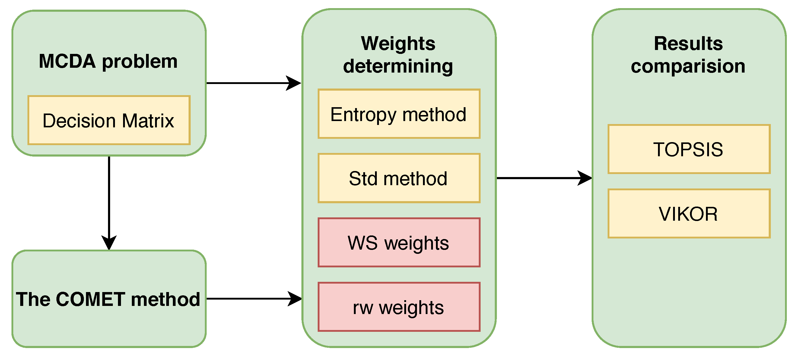Figure 1 presents the plan for the proposed research. We propose two new weighting methods which are based on ranking similarity coefficients. For these purposes, we present a comparative case study on the evaluation of electric bicycles. This is a continuation of previous work [54], where a modern Characteristic Object METhod (COMET) method was used, and a reference bicycle ranking was obtained. We compare the results for two proposed and two commonly used weighting method. Based on four different approaches for determining the relevance of criteria, we re-analyze the decision-making process using different standardization methods and Technique for Order of Preference by Similarity to Ideal Solution (TOPSIS) and VIKOR (in Serbian: VlseKriterijumska Optimizacija I Kompromisno Resenje) methods. The resulting rankings are then compared with a reference ranking that will help to determine the effectiveness of the investigated weighting methods. The main contribution of our research is, therefore, to propose two new approaches to the analysis of the relevance of decision-making criteria, and additionally to examine their effectiveness. The differences between the existing and proposed methods are significant and encourage further work in this direction.

The rest of the paper is organized as follows. Section 2 contains a brief introduction to fuzzy set theory, MCDA methods, correlation coefficients and normalization methods. The investigated study case is described in Section 3, which was divided into two parts, describing the data used for research (Section 3.1) and the research methodology (Section 3.2). Section 4 is devoted to the presentation of results and their discussion, which takes place in Section 4.1 and Section 4.2 for TOPSIS and VIKOR methods respectively. Finally, the conclusions are formulated in Section 5.

2. Preliminaries

2.1. Fuzzy Set Theory

The idea of Fuzzy Set Theory was introduced by Lofti Zadeh in [55]. Fuzzy Set Theory is used in many scientific fields and could be especially useful for solving MCDA problems [56,57,58]. Here we present some definitions and basic concepts of the Fuzzy Set Theory which are necessary to understand COMET method [59,60,61].

Definition 1.

The fuzzy set A in a certain non-empty space of solutions X is defined by (1).

$$A=\left\{\left(x,{\mu }_A\left(x\right)\right);x\in X\right\},$$

(1)

where

$${\mu }_A\left(x\right):X\to [0,1],$$

(2)

is a membership function of the fuzzy set A. This function indicates the degree of the membership of the element in the set A. ${\mu }_A\left(x\right)=1$ means full membership, $0<{\mu }_A\left(x\right)<1$ means partial membership and ${\mu }_A\left(x\right)=0$ means no membership at all.

Definition 2.

The triangular fuzzy number $A(a,m,b)$ is a fuzzy set which membership function is defined as followed (3):

$${\mu }_A(x,a,m,b)=\left\{\begin{array}{cc}0\hfill & x\le a\hfill \\ \frac{x-a}{m-a}\hfill & a\le x\le m\hfill \\ 1\hfill & x=m\hfill \\ \frac{b-x}{b-m}\hfill & m\le x\le b\hfill \\ 0\hfill & x\ge b\hfill \end{array}\right.$$

(3)

and fulfill characteristics (4) and (5):

$$x_1,x_2\in [a,m]\wedge x_2>x_1\Rightarrow {\mu }_A\left(x_2\right)>{\mu }_A\left(x_1\right)$$

(4)

$$x_1,x_2\in [m,b]\wedge x_2>x_1\Rightarrow {\mu }_A\left(x_2\right)<{\mu }_A\left(x_1\right)$$

(5)

Definition 3.

The support of a TFN—subset of the A set in which all elements have a non-zero membership value in the A set (6).

$$S\left(\tilde{A}\right)=x:{\mu }_{\tilde{A}}\left(x\right)>0=[a,b]$$

(6)

Definition 4.

The core of a TFN is a one-element fuzzy set (singleton) with membership value 1 (7).

$$C\left(\tilde{A}\right)=x:{\mu }_{\overline{A}}\left(x\right)=1=m$$

(7)

Definition 5.

The fuzzy rule—single fuzzy rule can be based on the Modus Ponens tautology. The reasoning process uses the $IF-THEN$, $OR$ and $AND$ logical connectives.

Definition 6.

The rule base—the rule base contains logical rules determining the relationships existing in the system between the input and output sets.

Definition 7.

The T-norm operator (intersection) is a function modeling the AND operation on two or more fuzzy numbers. T-norm is described by following properties: boundary (8), monotonicity (9), commutativity (10), associativity (11), for any $a,b,c,d\in [0,1].$

$$T(0,0)=0,T(a,1)=T(1,a)=a$$

(8)

$$T(a,b)<T(c,d)\iff ifa<candb<d$$

(9)

$$T(a,b)=T(b,a)$$

(10)

$$T(a,T(b,c\left)\right)=T\left(T\right(a,b),c)$$

(11)

Definition 8.

The S-norm operator or T-conorm is a function modeling the OR operator of two or more fuzzy numbers. It should fulfill the following properties: boundary (12), monotonicity (13), commutativity (14), associativity (15), for any $a,b,c,d\in [0,1].$

$$S(1,1)=1,S(a,0)=S(0,a)=a$$

(12)

$$S(a,b)<S(c,d)\iff ifa<candb<d$$

(13)

$$S(a,b)=S(b,a)$$

(14)

$$S(a,S(b,c\left)\right)=S\left(S\right(a,b),c)$$

(15)

2.2. Mcda Methods

2.2.1. COMET

The Characteristic Objects METhod (COMET) is based on fuzzy logic and triangular fuzzy sets. The accuracy of the COMET method was verified in previous works [20,30,62]. The formal notation of the COMET must be recalled based on [63,64,65], and Figure 2 presents the flowchart of the COMET method as summarizing.

Step 1. Definition of the space of the problem—the expert determines the dimensionality of the problem by selecting r criteria, $C_1,C_2,\dots ,C_r$. Then, a set of fuzzy numbers is selected for each criterion $C_i$, e.g., $\{{\tilde{C}}_{i1},{\tilde{C}}_{i2},\dots ,{\tilde{C}}_{i{c}_i}\}$ (16):

$$\begin{array}{c}{C}_1=\left\{{\tilde{C}}_{11},{\tilde{C}}_{12},\dots ,{\tilde{C}}_{1c_1}\right\}\\ C_2=\left\{{\tilde{C}}_{21},{\tilde{C}}_{22},\dots ,{\tilde{C}}_{2c_2}\right\}\\ \cdots \\ C_r=\left\{{\tilde{C}}_{r1},{\tilde{C}}_{r2},\dots ,{\tilde{C}}_{r{c}_r}\right\}\end{array}$$

(16)

where $C_1,C_2,\dots ,C_r$ are the ordinals of the fuzzy numbers for all criteria.

Step 2. Generation of the characteristic objects—the characteristic objects ($CO$) are obtained with the usage of the Cartesian product of the fuzzy numbers’ cores of all the criteria (17):

$$CO=\langle C\left(C_1\right)\times C\left(C_2\right)\times \cdots \times C\left(C_r\right)\rangle$$

(17)

As a result, an ordered set of all $CO$ is obtained (18):

$$\begin{array}{c}C{O}_1=\langle C\left({\tilde{C}}_{11}\right),C\left({\tilde{C}}_{21}\right),\dots ,C\left({\tilde{C}}_{r1}\right)\rangle \\ C{O}_2=\langle C\left({\tilde{C}}_{11}\right),C\left({\tilde{C}}_{21}\right),\dots ,C\left({\tilde{C}}_{r1}\right)\rangle \\ \cdots \\ C{O}_t=\langle C\left({\tilde{C}}_{1c_1}\right),C\left({\tilde{C}}_{2c_2}\right),\dots ,C\left({\tilde{C}}_{r{c}_r}\right)\rangle \end{array}$$

(18)

where t is the count of $CO$s and is equal to (19):

$$t=\prod _{i=1}^r{c}_i$$

(19)

Step 3. Evaluation of the characteristic objects—the expert determines the Matrix of Expert Judgment ($MEJ$) by comparing the $CO$s pairwise. The matrix is presented below (20):

$$MEJ=\left(\begin{array}{cccc}{\alpha }_{11}& {\alpha }_{12}& \cdots & {\alpha }_{1t}\\ {\alpha }_{21}& {\alpha }_{22}& \cdots & {\alpha }_{2t}\\ \cdots & \cdots & \cdots & \cdots \\ {\alpha }_{t1}& {\alpha }_{t2}& \cdots & {\alpha }_{tt}\end{array}\right)$$

(20)

where ${\alpha }_{ij}$ is the result of comparing $C{O}_i$ and $C{O}_j$ by the expert. The function $f_{exp}$ denotes the mental judgment function of the expert. It depends solely on the knowledge of the expert. The expert’s preferences can be presented as (21):

$${\alpha }_{ij}=\left\{\begin{array}{c}0.0,f_{exp}\left(C{O}_i\right)<f_{exp}\left(C{O}_j\right)\hfill \\ 0.5,f_{exp}\left(C{O}_i\right)=f_{exp}\left(C{O}_j\right)\hfill \\ 1.0,f_{exp}\left(C{O}_i\right)>f_{\exp }\left(C{O}_j\right)\hfill \end{array}\right.$$

(21)

After the MEJ matrix is prepared, a vertical vector of the Summed Judgments ($SJ$) is obtained as follows (22):

$$S{J}_i=\sum _{j=1}^t{\alpha }_{ij}$$

(22)

Eventually, the values of preference are approximated for each characteristic object. As a result, a vertical vector P is obtained, where the i-th row contains the approximate value of preference for $C{O}_i$.

Step 4. The rule base—each characteristic object and its value of preference is converted to a fuzzy rule as (23):

$$IFC\left({\tilde{C}}_{1i}\right)ANDC\left({\tilde{C}}_{2i}\right)AND\dots THEN{P}_i$$

(23)

In this way, a complete fuzzy rule base is obtained.

Step 5. Inference and the final ranking—each alternative is presented as a set of crisp numbers, e.g., $A_i=\{{\alpha }_{i1},{\alpha }_{i2},{\alpha }_{ri}\}$. This set corresponds to the criteria $C_1,C_2,\dots ,C_r$. Mamdani’s fuzzy inference method is used to compute the preference of the i-th alternative. The rule base guarantees that the obtained results are unequivocal. The bijection makes the COMET completely rank reversal free.

2.2.2. TOPSIS

The TOPSIS method is a simple MCDA technique used in many practical problems. Thanks to its simplicity of use it is widely used in solving multi-criteria problems. Below we present its algorithm [66]. We assume that we have decision matrix with m alternatives and n criteria is represented as $X={\left(x_{ij}\right)}_{m\times n}$.

Step 1. Calculate the normalized decision matrix. The normalized values $r_{ij}$ calculated according to Equation (39) for profit criteria and (40) for cost criteria. We use this normalization method, because [67] shows that it performs better that classical vector normalization.

$$r_{ij}=\frac{x_{ij}-mi{n}_j\left(x_{ij}\right)}{ma{x}_j\left(x_{ij}\right)-mi{n}_j\left(x_{ij}\right)}$$

(24)

$$r_{ij}=\frac{ma{x}_j\left(x_{ij}\right)-x_{ij}}{ma{x}_j\left(x_{ij}\right)-mi{n}_j\left(x_{ij}\right)}$$

(25)

Step 2. Calculate the weighted normalized decision matrix $v_{ij}$ according to Equation (26).

$$v_{ij}=w_i{r}_{ij}$$

(26)

Step 3. Calculate Positive Ideal Solution (PIS) and Negative Ideal Solution (NIS) vectors. PIS is defined as maximum values for each criterion (27) and NIS as minimum values (28). We do not need to split criteria into profit and cost here, because in step 1 we use normalization which turns cost criteria into profit criteria.

$$v_j^{+}=\{v_1^{+},v_2^{+},\cdots ,v_n^{+}\}=\left\{ma{x}_j\left(v_{ij}\right)\right\}$$

(27)

$$v_j^{-}=\{v_1^{-},v_2^{-},\cdots ,v_n^{-}\}=\left\{mi{n}_j\left(v_{ij}\right)\right\}$$

(28)

Step 4. Calculate distance from PIS and NIS for each alternative. As shows Equations (29) and (30).

$$D_i^{+}=\sqrt{\sum _{j=1}^n{(v_{ij}-v_j^{+})}^2}$$

(29)

$$D_i^{-}=\sqrt{\sum _{j=1}^n{(v_{ij}-v_j^{-})}^2}$$

(30)

Step 5. Calculate each alternative’s score according to Equation (31). This value is always between 0 and 1, and the alternatives which got values closer to 1 are better.

$$C_i=\frac{D_i^{-}}{D_i^{-}+D_i^{+}}$$

(31)

2.2.3. VIKOR

The VIKOR method, similarly to the TOPSIS method, is based on distance measurements. In this approach a compromise solution is sought. The description of the method will be quoted according to [68,69]. Let us say that we have decision matrix with m alternatives and n criteria is represented as $X=f_{ij}{\left(A_i\right)}_{m\times n}$.

Step 1. Determine the best $f_i^{*}$ and the worth $f_i^{-}$ values for each criteria functions. Use (32) for profit criteria and (33) for cost criteria.

$$f_j^{*}=\underset{i}{max}{f}_{ij},f_j^{-}=\underset{i}{min}{f}_{ij}$$

(32)

$$f_j^{*}=\underset{i}{min}{f}_{ij},f_j^{-}=\underset{i}{max}{f}_{ij}$$

(33)

Step 2. Calculate the $S_i$ and $R_i$ values by Equations (34) and (35).

$$S_i=\sum _{j=1}^n{w}_j\left(f_j^{*}-f_{ij}\right)/\left(f_j^{*}-f_j^{-}\right)$$

(34)

$$R_i=\underset{j}{max}\left[w_j\left(f_j^{*}-f_{ij}\right)/\left(f_j^{*}-f_j^{-}\right)\right]$$

(35)

Step 3. Compute the $Q_i$ values using Equation (36).

$$Q_i=v\left(S_i-S^{*}\right)/\left(S^{-}-S^{*}\right)+(1-v)\left(R_i-R^{*}\right)/\left(R^{-}-R^{*}\right)$$

(36)

where

• $S^{*}={min}_i{S}_i,S^{*}={min}_i{S}_i$
• $R^{*}={min}_i{R}_i,R^{*}={max}_i{R}_i$

and v is introduced as a weigh for the strategy “majority of criteria”. We use $v=0.5$ here.

Step 4. Rank alternatives, sorting by the values S, R, Q in ascending order. Result is three ranking lists.

Step 5. Normally, we should use S, R, Q ranking lists to propose the compromise solution or set of compromise solutions, as showed in [69,70]. However, in this paper would be used only Q ranking list.

2.3. Correlation Coefficients

Correlation coefficients make it possible to compare obtained results and determine how similar they are. In this paper, we would use the weighted Spearman correlation coefficient (37) and the rank similarity coefficient (38) to determine how similar obtained with COMET rankings to reference rankings.

2.3.1. Weighted Spearman’s Rank Correlation Coefficient

For a sample of size N, the rank values $x_i$ and $y_i$ is defined as (37). In this approach, the positions at the top of both rankings are more important. The weight of significance is calculated for each comparison. It is the element that determines the main difference to the Spearman’s rank correlation coefficient, which examines whether the differences appeared and not where they appeared.

$$r_w=1-\frac{6{\sum }_{i=1}^N{(x_i-y_i)}^2((N-x_i+1)+(N-y_i+1))}{N^4+N^3-N^2-N}$$

(37)

2.3.2. Rank Similarity Coefficient

For a sample of size N, the rank values $x_i$ and $y_i$ is defined as (38) [71]. It is an asymmetric measure. The weight of a given comparison is determined based on the significance of the position in the first ranking, which is used as a reference ranking during the calculation.

$$WS=1-\sum _{i=1}^N{2}^{-x_i}\frac{|x_i-y_i|}{max\left(\right|x_i-1|,|x_i-N\left|\right)}$$

(38)

2.4. Normalization Methods

In the literature, there is no clear assignment to which decision-makers’ methods of data normalization are used. This situation poses a problem, as it is necessary to consider the influence of particular normalization on the result. The most common normalization methods in MCDA methods can be divided into two groups [72], i.e., methods designed to profit (39), (41), (43) and (45) and cost criteria (40), (42), (44) and (46).

The minimum-maximum method—in this approach, the greatest and the least values in the considered set are used. The formulas are described as follows (39) and (40):

$$r_{ij}=\frac{x_{ij}-mi{n}_j\left(x_{ij}\right)}{ma{x}_j\left(x_{ij}\right)-X_{min}}$$

(39)

$$r_{ij}=\frac{ma{x}_j\left(x_{ij}\right)-x_{ij}}{ma{x}_j\left(x_{ij}\right)-mi{n}_j\left(x_{ij}\right)}$$

(40)

The maximum method—in this technique, only the greatest value in the considered set is used. The formulas are described as follows (41) and (42):

$$r_{ij}=\frac{x_{ij}}{ma{x}_j\left(x_{ij}\right)}$$

(41)

$$r_{ij}=1-\frac{x_{ij}}{ma{x}_j\left(x_{ij}\right)}$$

(42)

The sum method—in this method, the sum of all values in the considered set is used. The formulas are described as follows (43) and (44):

$$r_{ij}=\frac{x_{ij}}{{\sum }_{i=1}^m{x}_{ij}}$$

(43)

$$r_{ij}=\frac{\frac{1}{x_{ij}}}{{\sum }_{i=1}^m\frac{1}{x_{ij}}}$$

(44)

The vector method—in this method, the square root of the sum of all values. The formulas are described as follows (45) and (46):

$$r_{ij}=\frac{x_{ij}}{\sqrt{{\sum }_{i=1}^m{x}_{ij}^2}}$$

(45)

$$r_{ij}=1-\frac{x_{ij}}{\sqrt{{\sum }_{i=1}^m{x}_{ij}^2}}$$

(46)

2.5. Weighting Methods

2.5.1. Entropy Method

According to [73], entropy method is based on a measure of uncertainty in the information. It is calculated using Equations (47)–(49) below.

$$p_{ij}=\frac{x_{ij}}{{\sum }_{i=1}^m{x}_{ij}}i=1,...,m;j=1,...,n$$

(47)

$$E_j=-\frac{{\sum }_{i=1}^m{p}_{ij}ln\left(p_{ij}\right)}{ln\left(m\right)}j=1,...,n$$

(48)

$$w_j=\frac{1-E_j}{{\sum }_{i=1}^n(1-E_i)}j=1,...,n$$

(49)

2.5.2. Standard Deviation Method

This method is similar to entropy at some point, and assigns small weights to an attribute which has similar values across alternatives. The SD method defined with Equations (50) and (51), where $w_j$ is weight of criteria and ${\sigma }_j$ is standard deviation [73].

$${\sigma }_j=\sqrt{\frac{{\sum }_{i=1}^m\left(x_{ij}-{\left.\overline{x_j}\right)}^2\right.}{m}}j=1,\dots ,n$$

(50)

$$w_j={\sigma }_j/\sum _{j=1}^n{\sigma }_{j}j=1,\dots ,n$$

(51)

3. Study Case

3.1. Materials

The material used for this case study will be the data from the article [54], which concerns the assessment of preferences for electric city bikes. For the analysis, eight criteria were used, which are presented in detail in

Table 1. Selected criteria $C_1$–$C_8$ and their characteristic values {low, medium, high} [54].

${\mathit{C}}_{\mathit{i}}$	Name	Unit	Low	Medium	High
$C_1$	battery capacity	Ah	4	9	15
$C_2$	charging time	hours	3	5	8
$C_3$	number of gears	units	1	7	21
$C_4$	engine power	W	250	350	500
$C_5$	maximum speed	km/h	20	27	35
$C_6$	range	km	20	60	100
$C_7$	weight	kg	10	20	25
$C_8$	price	USD	300	2500	6300

. It should be noted that each criterion has a different numerical domain. This will be of particular importance when determining the relevance weighting of criteria. In Table 1, there are also characteristic values determined for particular criteria, which is one of the most important steps in the COMET method.

Visualization of linguistic values, i.e., low, medium and high, is shown in Figure 3. All the presented fuzzy numbers are asymmetrical because they are matched to the data distributions identified by the expert. The identified structural model was transformed into a monolithic model, which was only auxiliary. The values of the preference, and thus the rankings of the identified decision-making sets, remained unchanged.

In our work, we focus only on those alternatives that were described with complete information. Therefore, 55 alternatives that are presented in detail in

Table 2. Alternatives description and preference.

${\mathit{A}}_{\mathit{i}}$	Name	${\mathit{C}}_1$	${\mathit{C}}_2$	${\mathit{C}}_3$	${\mathit{C}}_4$	${\mathit{C}}_5$	${\mathit{C}}_6$	${\mathit{C}}_7$	${\mathit{C}}_8$	P	Rank
$A_1$	2017 Raleigh Detour iE	11.6	4	9	250	32	80	21.7	2399	0.5779	26
$A_2$	BESV CF1	8.4	5	10	250	28.8	64	22.4	1799	0.4810	46
$A_3$	BESV PSA1	10.5	5	7	250	30.4	72	19.5	1999	0.5569	35
$A_4$	Blix Aveny	11	3	7	350	32	96	23.5	1899	0.6849	2
$A_5$	Blix Sol	11	3	7	350	32	88	22	1599	0.6870	1
$A_6$	California Bicycle S	8	4	1	250	32	56	22.6	2499	0.3669	55
$A_7$	Cannondale E-Rigid	11	3.5	8	350	32	100	22.6	3490	0.6280	9
$A_8$	Coboc ONE Soho	9.6	3	1	250	24.8	88	13.1	5520	0.4016	52
$A_9$	CUBE Cross Pro 400	11	3.5	9	250	32	96	22.7	2599	0.6236	11
$A_{10}$	Desiknio Pinion Classic	7	3	6	250	24.8	80	15.7	6135	0.3945	53
$A_{11}$	Desiknio Single Urban	7	3	1	250	24.8	80	13.1	4415	0.3898	54
$A_{12}$	EcoMotion Tour e-Road	10.4	4	7	350	32	83	20.2	1299	0.6763	4
$A_{13}$	E-Glide SS	10.4	5	1	350	32	56	17.1	1099	0.4893	44
$A_{14}$	E-Glide ST	11.4	6	10	500	32	80	24.4	1699	0.5838	25
$A_{15}$	e-Joe Gadis	11	5	7	350	32	72	24.9	1699	0.5555	36
$A_{16}$	E-Lux Monaco	10.5	6	9	500	32	88	24.8	1995	0.5912	23
$A_{17}$	Emazing Coeus 73h3h	8.7	4	7	350	32	88	20.2	1800	0.6591	5
$A_{18}$	Emazing Selene 73h3h	8.7	4	7	350	32	88	21.9	2000	0.6336	8
$A_{19}$	Espin Flow	11.6	4.5	8	350	35	80	24.3	1888	0.6095	17
$A_{20}$	EUNORAU E-TORQUE	12.5	5	7	350	32	72	24.6	1599	0.5694	32
$A_{21}$	eVox KAB 375	7.8	4	8	350	35	100	20.4	2199	0.6831	3
$A_{22}$	Gazelle Avenue C8	14	4	8	250	32	100	23.8	2999	0.6167	13
$A_{23}$	Gazelle CityZen C8 HM	11	3.5	8	350	32	94	23.1	2999	0.6204	12
$A_{24}$	Gazelle CityZen T9 HMB	13.4	4	9	350	32	100	24.1	3499	0.6089	18
$A_{25}$	GenZe 200 Series	9.6	3.5	8	350	32	56	22.6	1899	0.5399	39
$A_{26}$	IZIP E3 Brio	11.6	5.5	7	250	32	80	25	1699	0.5600	33
$A_{27}$	IZIP E3 Loma	11	5.5	7	250	32	80	24.9	1699	0.5582	34
$A_{28}$	Juiced OceanCurrent	8.8	4	8	500	35	64	23.1	1299	0.6144	14
$A_{29}$	Junto Gen 1	11.6	6	11	350	32	96	22.1	2222	0.6140	15
$A_{30}$	Kalkhoff Agattu B7	11	3.5	7	250	32	100	24	2499	0.6353	7
$A_{31}$	Optibike Rocky Mount.	11.6	5	11	500	35	96	24.4	3995	0.5768	27
$A_{32}$	Orbea Katu-E 10	11	3.5	8	250	32	96	22.9	2999	0.6114	16
$A_{33}$	Populo Lift V2	8.7	4.5	7	250	32	56	22.1	1399	0.5273	41
$A_{34}$	Populo Scout	13	4.5	8	350	32	80	24.7	1699	0.6010	22
$A_{35}$	Populo Sport	10.4	3	1	250	32	48	15.7	999	0.5028	43
$A_{36}$	Populo Sport V3	8.7	4.5	1	250	32	56	16.7	999	0.4813	45
$A_{37}$	Propella 2.2 7-Speed	6.8	3	7	250	28.8	56	16.8	1299	0.5486	37
$A_{38}$	Propella V2.0 Single-Speed	6.8	3	1	250	25.6	56	13.6	1199	0.4495	48
$A_{39}$	PUBLIC D8 Electric	8.8	4.5	8	350	32	88	24.8	2199	0.5841	24
$A_{40}$	Pure Cycles Volta 8-Speed	5.8	4	8	250	32	40	17	1999	0.4433	49
$A_{41}$	Raleigh Sprite iE	8.8	5	7	350	32	64	24.5	1899	0.5116	42
$A_{42}$	Raleigh Superbe iE	8.8	4.5	7	350	32	64	22.7	1799	0.5450	38
$A_{43}$	Riese, Müller Mixte	13.4	3.5	10	350	32	100	21.9	3879	0.6238	10
$A_{44}$	Riese, Müller NuVinci	11	3.5	1	250	32	100	24.8	4489	0.4592	47
$A_{45}$	Schwinn Monroe 250	11.6	4.5	1	250	32	72	18.8	1199	0.5335	40
$A_{46}$	Schwinn Monroe 350	14	6	1	350	32	88	20.4	1499	0.5732	28
$A_{47}$	Scott E-Sub Evo	11	3.5	8	350	32	100	22.4	4199	0.6060	20
$A_{48}$	Shaofu 6AH	4.4	3	1	350	25	20	12	390	0.4261	50
$A_{49}$	Specialized Como 2.0	12.8	3.5	9	250	32	96	21.5	2600	0.6411	6
$A_{50}$	Specialized Como 3.0	12.8	4	9	250	32	80	20.7	2950	0.5711	31
$A_{51}$	Specialized Vado 3.0	12.5	3.5	10	250	32	100	24.5	3200	0.6027	21
$A_{52}$	Trek Lift+ Lowstep	11.6	4	10	250	32	80	20.3	2799	0.5718	29
$A_{53}$	Trek Neko+	11.6	4	10	250	32	80	19.1	2999	0.5717	30
$A_{54}$	VoltBike Urban	13	5.5	6	350	32	80	23.4	1199	0.6085	19
$A_{55}$	Xiaomi QiCycle	5.8	3	3	250	20	45	14.5	950	0.4063	51

will be analyzed. Table 2 shows the full decision matrix, which is contained in columns from $C_1$ to $C_8$. There is also presented information about the value of preferences and the position in the ranking of each of the examined bicycles. For example, the most attractive bicycle turned out to be Blix Sol, i.e., alternative $A_5$, which received a rating of 0.6870. California Bicycle S, which received a rating of 0.3669 and the last place in the ranking, was indicated as the least attractive bicycle. It is worth noting the differences between some alternatives are relatively low, where for example, the second position in the ranking has a rating worse by only 0.0021.

It is worth recalling that the obtained results come from a method that does not require a model of knowledge of the significance of decision-making criteria to be determined. The expert identifies the whole model by comparing pairs of characteristic objects. In this way, an indirect identification takes place, and the models obtained in this way are well suited to complex non-linear problems. Thanks to this, and based on Table 2, we will propose two approaches to identify the relevance of criteria in Section 3.2.

3.2. Methods

To determine the relevance of the criteria, a reference ranking was used. It was created using the model identified by the COMET method. In the next step, we set eight rankings which are created by successive exclusions of individual component criteria from the primary model. Each such ranking has exactly seven active criteria and one excluded criterion.

Table 3. Correlation with reference ranking when one criterion excluded.

Excluding	1	2	3	4	5	6	7	8	9	10	${\mathit{r}}_{\mathit{w}}$	$\mathit{WS}$
$none$	$A_5$	$A_4$	$A_{21}$	$A_{12}$	$A_{17}$	$A_{49}$	$A_{30}$	$A_{18}$	$A_7$	$A_{43}$	1.0000	1.0000
$C_1$	$A_{28}$	$A_{21}$	$A_5$	$A_4$	$A_{12}$	$A_{17}$	$A_{43}$	$A_{31}$	$A_7$	$A_{18}$	0.8244	0.9616
$C_2$	$A_{14}$	$A_{31}$	$A_{29}$	$A_{16}$	$A_{28}$	$A_{43}$	$A_{12}$	$A_{21}$	$A_5$	$A_{24}$	0.7513	0.8377
$C_3$	$A_5$	$A_4$	$A_{28}$	$A_{12}$	$A_{43}$	$A_{21}$	$A_7$	$A_{17}$	$A_{23}$	$A_{31}$	0.8011	0.9854
$C_4$	$A_{49}$	$A_5$	$A_{43}$	$A_{53}$	$A_{52}$	$A_{50}$	$A_9$	$A_4$	$A_{12}$	$A_1$	0.7801	0.9208
$C_5$	$A_{43}$	$A_5$	$A_4$	$A_{28}$	$A_{12}$	$A_{31}$	$A_{49}$	$A_{24}$	$A_7$	$A_{23}$	0.8190	0.9558
$C_6$	$A_{28}$	$A_5$	$A_{43}$	$A_{12}$	$A_{31}$	$A_4$	$A_{25}$	$A_{21}$	$A_{49}$	$A_{14}$	0.7176	0.9459
$C_7$	$A_4$	$A_{28}$	$A_5$	$A_{31}$	$A_{43}$	$A_{24}$	$A_{23}$	$A_{34}$	$A_{19}$	$A_7$	0.8429	0.9284
$C_8$	$A_{43}$	$A_{31}$	$A_{47}$	$A_5$	$A_7$	$A_{24}$	$A_4$	$A_{28}$	$A_{23}$	$A_{21}$	0.7897	0.9076

presents the main ranking without exclusions and eight derivative rankings with their ten initial alternatives. The most important information contained in this table is the value of the similarity coefficient between the main ranking and individual derivative rankings. For this purpose, two measures of $r_w$ and $WS$ were used. The highest value of $r_w$ was recorded for the ranking that excluded the $C_7$ criterion from the main model (value 0.8429). The smallest value was obtained for the ranking that excluded criterion $C_6$ (value 0.7176). This means that the $C_6$ criterion had a more significant impact on the ranking change than the $C_7$ criterion, so it was more significant than the $r_w$ criterion. The lowest value is obtained for criterion $C_2$, i.e., 0.8377, so based on the $WS$ coefficient, the most important is criterion $C_2$ and the least important is criterion $C_3$. It should be reminded here that both coefficients have a different paradigm of determining the similarity of the two rankings. Therefore, both these coefficients will be used for further investigation.

The $r_w$ coefficient indicated that the most important criterion is the range and the least important criterion is the weight of the bike. It is common sense that this is in line with the expectations of many consumers. The most important criterion is the charging time expressed in hours, and the least important is the number of gears. It should be noted that in both cases, the battery capacity is a less important parameter in this case than the range of the bicycle. It can be explained by the fact that a battery with a specific capacity does not always guarantee the same distance and this attribute can be less important than range. Figure 4 presents the similarity of the reference and derivative rankings.

Due to the nature of both coefficients, we propose the following formula (52) to calculate the significance weights of the individual criteria:

$$w_i=\frac{1-x_i}{{\sum }_{j=1}^{N}1-x_j},$$

(52)

where N means the number of all criteria, $w_i$ is a i-th weights of criterion $C_i$, and $x_i$ is i-th coefficient ($WS$ or $r_w$). This gives us two different approaches to the importance of weights, which will be compared with entropy (49) and standard deviation (51) methods.

Table 4. Weights determined with different methods.

${\mathit{C}}_{\mathit{i}}$	${\mathit{r}}_{\mathit{w}}$ Weights	$\mathit{WS}$ Weights	Entropy Method	Std Method
$C_1$	0.1049	0.0690	0.0627	0.0017
$C_2$	0.1486	0.2914	0.0589	0.0007
$C_3$	0.1188	0.0262	0.3854	0.0025
$C_4$	0.1313	0.1423	0.0648	0.0569
$C_5$	0.1081	0.0794	0.0109	0.0022
$C_6$	0.1687	0.0972	0.0795	0.0146
$C_7$	0.0939	0.1286	0.0393	0.0028
$C_8$	0.1256	0.1660	0.2984	0.9185

provides detailed results of the relevance weights obtained using two new and two traditional methods for determining the relevance of criteria.

To better compare the obtained criteria weights, they are shown in Figure 5. The significance weights determined by means of the $r_w$ coefficient are characterized by quite equal distribution of significance. The most significant criterion is the range with weight 0.1687 and the least significant is the weight with weight 0.0939. Greater differences between the individual weights occur with the approach using the $WS$ coefficient. In this case charging time (0.2914) is the most important and the number of gears is the least important (0.0262). Using the entropy of information approach, we get as the most important criterion the number of gears (0.3854) and the least important criterion is the maximum speed (0.0109). The most asymmetrical in its assessment is the method based on standard deviation where the price has a significance equal to 0.9185. According to this approach, the least important parameter is the charging time. The results obtained using information entropy and standard deviation are less effective than our proposed approaches, which will be proven in the next section.

4. Results and Discussion

4.1. TOPSIS

To check the effectiveness of the four criteria weighting methods, the first TOPSIS method will be used, where 55 electric bicycles will be evaluated using different normalization methods with each of the four methods to identify the significance of the weights. Figure 6, Figure 7, Figure 8 and Figure 9 show a comparison of reference ranking and rankings determined by TOPSIS method, selected normalizations and ways of determining criterion significance. In case of perfect compatibility, the black dots should completely cover the blue line. Figure 6 shows visualizations of the results using minimax normalization. Visually, the best representation was achieved using the scales determined by the $r_w$ approach. The ranking circle was also well reflected by using the $WS$ approach. At the same time, the entropy and standard deviation method reflected best the tail of the ranking. This is confirmed by the numerical values presented in

Table 5. Comparison of the results from the reference ranking and the ranking obtained by using TOPSIS and different normalization techniques.

Normalization	Weighted Method	${\mathit{r}}_{\mathit{w}}$	$\mathit{WS}$
minmax	$r_w$ weights	0.8959	0.9831
	$WS$ weights	0.2759	0.9415
	Entropy weights	0.3887	0.6301
	Std weights	−0.2079	0.6634
max	$r_w$ weights	0.9283	0.9897
	$WS$ weights	0.4002	0.9698
	Entropy weights	0.3369	0.6111
	Std weights	−0.2079	0.6634
sum	$r_w$ weights	0.4204	0.8302
	$WS$ weights	−0.0655	0.7783
	Entropy weights	0.0407	0.4963
	Std weights	−0.2162	0.6626
vector	$r_w$ weights	0.7311	0.9675
	$WS$ weights	0.1242	0.9200
	Entropy weights	0.2651	0.7195
	Std weights	−0.2079	0.6634

. the method based on the $r_w$ coefficient undoubtedly did best in this aspect.

Then, Figure 7 shows a comparison of results obtained using normalization max type. The $r_w$ method again proved to be the most similar to the reference ranking results obtained with the COMET method. This is confirmed by the numbers presented in Table 5. In this case, both coefficients also inform us about the advantage of the $WS$ method over the entropy and standard deviation methods.

Another normalization based on the sum does not bring such unambiguous results as in the two previous cases. In all four methods presented in Figure 8, the dispersion is higher than in the previous cases. However, based on the data from Table 5, it can be concluded that the $r_w$ significance test method received relatively good results. It should be reminded here once again that the ideal situation is when all the dots are exactly on the blue line. This means that the two rankings are identical, which was well visible in Figure 7 when using the $r_w$ approach weights was the closest to this situation. At that time, the rankings’ similarity coefficients were 0.9283 and 0.9897, respectively.

The last examined case is vector normalization, presented in Figure 9, which again gives the best results in the $r_w$ ratio approach, where similarity measures are 0.7311 and 0.9675, respectively. Again, the least effective is the standard deviation approach. When comparing rankings using $r_w$ ratio, entropy approach is more effective than $WS$ approach. However, using $WS$ coefficient, the situation is the opposite. This is due to better matching of the ranking front in the $WS$ method than in the case of entropy. It is characteristic for the $WS$ ratio because it is the top of the ranking that is most important there, and the ratio itself is an asymmetric measure.

The complete list of results using the similarity of rankings is presented in Table 5. The normalization methods that best managed to reconstruct the initial ranking were minmax and max, and the worst managed to be the sum-based method.

To summarize the effectiveness of the proposed methods and standard approaches, we present Figure 10. This is a visualization of the results obtained with a $r_w$ ratio. Its value can range from −1 to 1. As we can see, for all types of standardization, the method based on the standard deviation is the least effective. The $r_w$ ratio method proposed in our article works most effectively as an alternative approach. The entropy method and our second proposition are poorly matched when using the $r_w$ similarity measure. However, the effectiveness advantage of the $r_w$ approach is undeniable.

When using the second-ranking matching indicator $WS$, one should pay attention to its different nature. In this case, the values may vary from zero to one. Figure 11 shows a comparison of the proposed approaches. Again, the most effective approach seems to be the $r_w$ weighting approach. In contrast to the previous list, the $WS$ weighting method came second. Interestingly, the method based on standard deviation was also used in three out of four cases and obtained better results than those obtained using entropy. In the analyzed case study, both comparative approaches indicate the highest efficiency using the $r_w$ ratio approach. In the next section, we will examine the efficiency of the set significance criteria using the example of the VIKOR method.

4.2. VIKOR

The next stage of checking the effectiveness of the proposed approaches will be based on the use of the VIKOR method without normalization and with four types of it. Although the method does not require the use of normalization, quite often one can meet the opinion that it is convicted to obtain better results. For readability of the paper, the drawings containing comparisons of the results from the reference ranking and the ranking obtained by using VIKOR are shown in the Appendix A. In Figure A1, all methods of determining the significance of the weights indicate high dispersion. This is the first case when entropy proves to be more effective and moreover with both parameters of ranking similarity measurement. In this case, the weakest match was obtained with the $WS$ coefficient. However, it should be emphasized that all obtained results indicate low effectiveness of the methods used.

Much lower dispersion is achieved when standardizing the decision matrix with the minmax method. The VIKOR method then has a much better matching of results than without normalization. This is visible in Figure A2, and the detailed measures of the matching are presented in

Table 6. Comparison of the results from the reference ranking and the ranking obtained by using VIKOR and different normalization techniques.

Normalization	Weighted Method	${\mathit{r}}_{\mathit{w}}$	$\mathit{WS}$
none	$r_w$ weights	0.4447	0.3525
	$WS$ weights	0.0124	0.2462
	Entropy weights	0.4802	0.4151
	Std weights	0.1514	0.3822
minmax	$r_w$ weights	0.8032	0.9640
	$WS$ weights	0.5124	0.9792
	Entropy weights	0.5091	0.6933
	Std weights	−0.1965	0.6596
max	$r_w$ weights	0.8032	0.9640
	$WS$ weights	0.5124	0.9792
	Entropy weights	0.5091	0.6933
	Std weights	−0.1965	0.6596
sum	$r_w$ weights	0.7927	0.9642
	$WS$ weights	0.2498	0.9188
	Entropy weights	0.5256	0.8346
	Std weights	−0.1917	0.6598
vector	$r_w$ weights	0.8032	0.9640
	$WS$ weights	0.5124	0.9792
	Entropy weights	0.5091	0.6933
	Std weights	−0.1965	0.6596

. The $WS$-based method is slightly more effective when testing the matching by $WS$ coefficient than the $r_w$-based approach. The weakest results were obtained using a method based on standard deviation. Identical results are obtained using max and vector normalizations. Figure A3 and Figure A5 return precisely the same results despite using a different normalization method. Thus, both cases are entirely equivalent.

The last tested normalization is a sum, where the results are presented in Figure A4. In this case, we obtain results similar to those of minmax, max and vector normalizations. The difference is that the effectiveness of the approach based on the $WS$ is deteriorated when using both meters. Detailed results of the analysis are presented in Table 6.

Summary of the analyses based on the $r_w$ coefficient is presented in Figure 12. Using any standardization, the determination of the significance of criteria with $r_w$ proves to be the most effective. The weakest approach was the one based on the standard deviation when we use any transformation of the decision matrix. Using VIKOR without normalization, the best result was obtained using the method based on entropy. However, it should be remembered that all the obtained results were much weaker. As many as three cases returned the same value. However, the highest effectiveness again falls to the approach based on $r_w$ coefficient.

When analyzing the data in Figure 13 we get very similar results. Again, without the use of techniques transforming the decision matrix, entropy turns out to be the best in the other two cases, the two most effective methods are those based on ranking similarity coefficients. The weakest approach is again, a standard deviation.

5. Conclusions

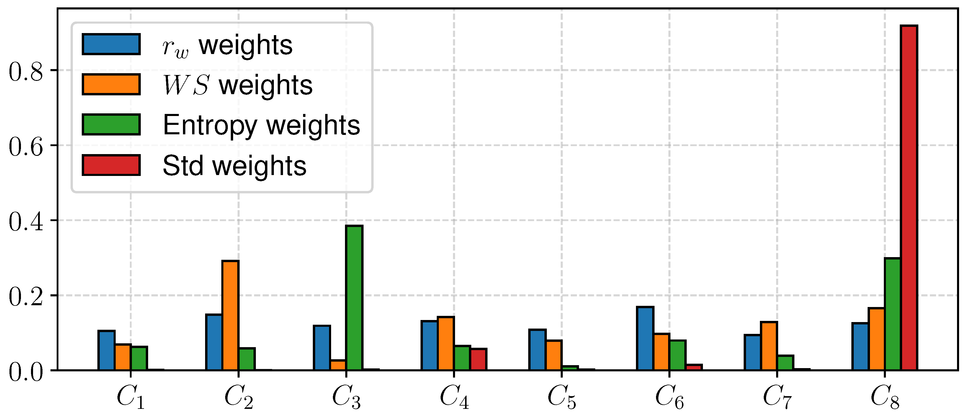
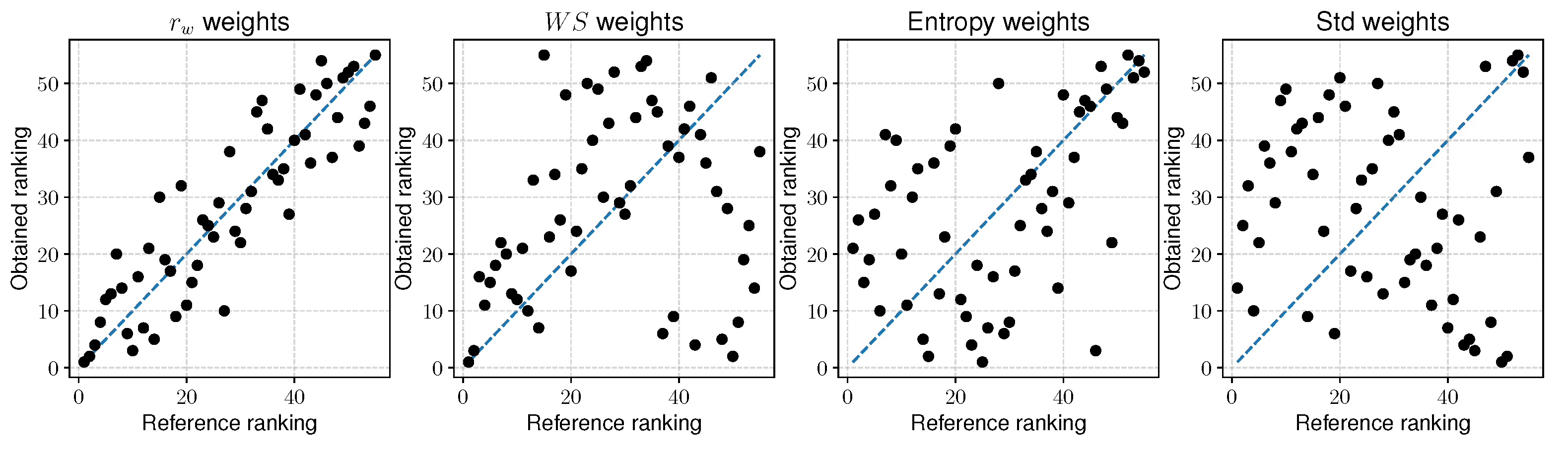
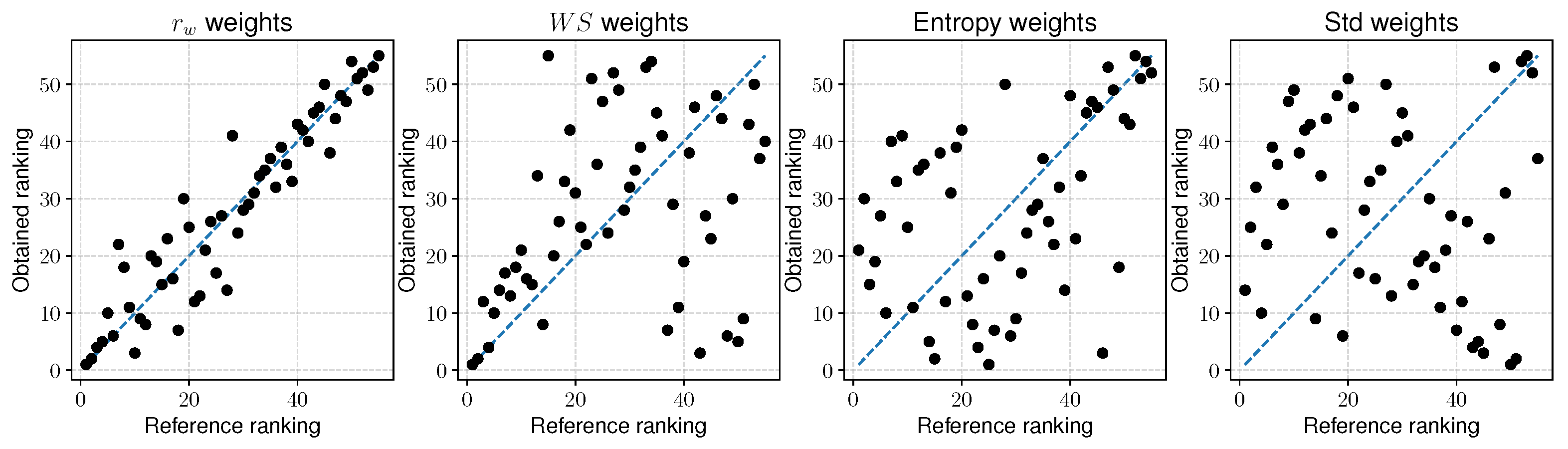
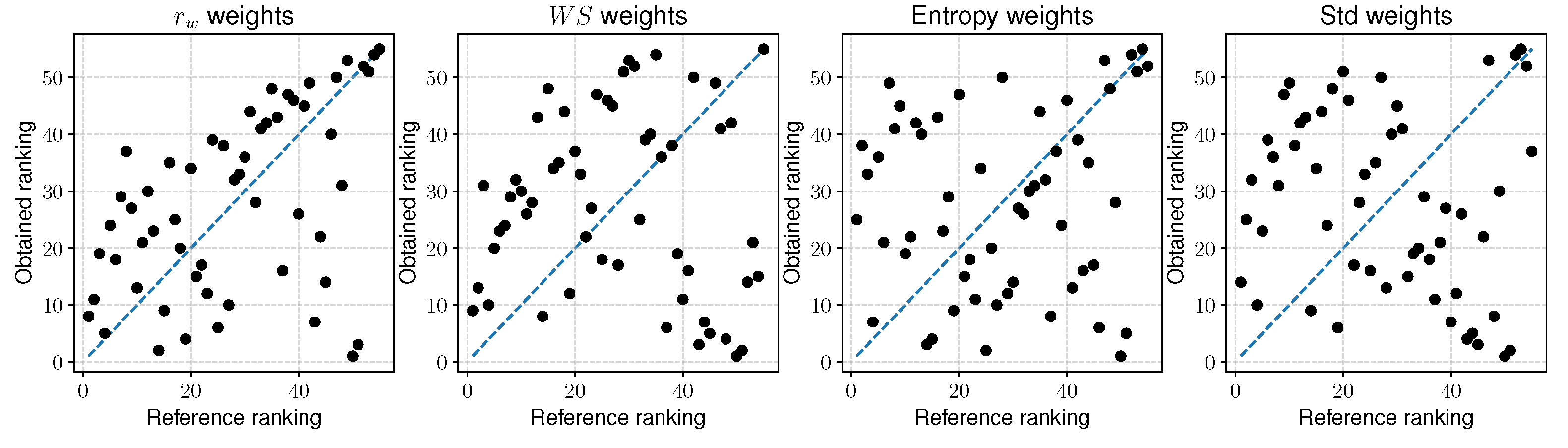
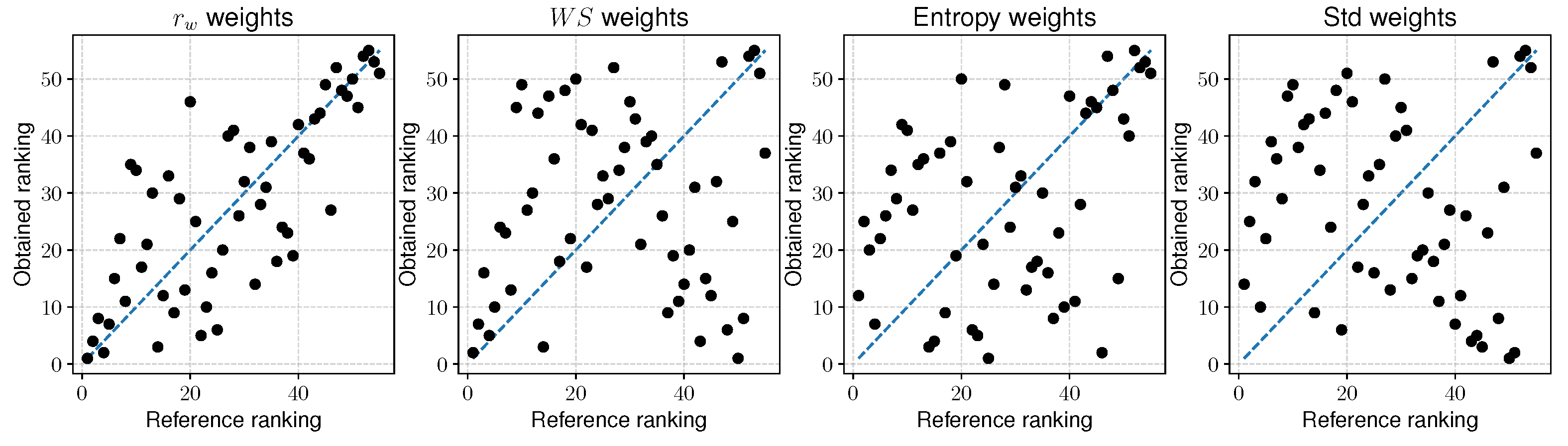
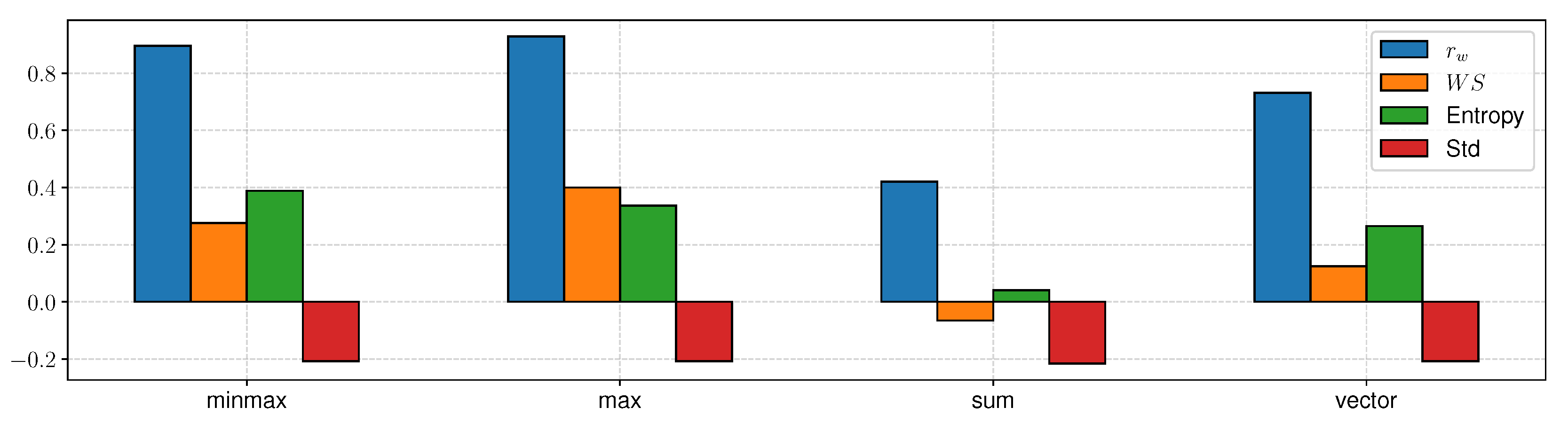
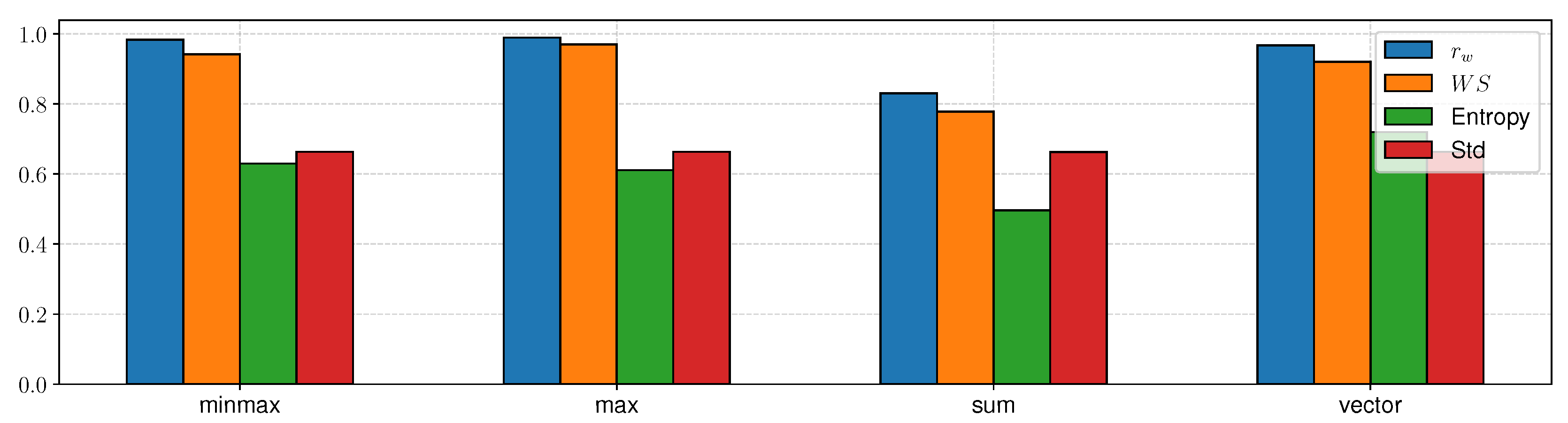
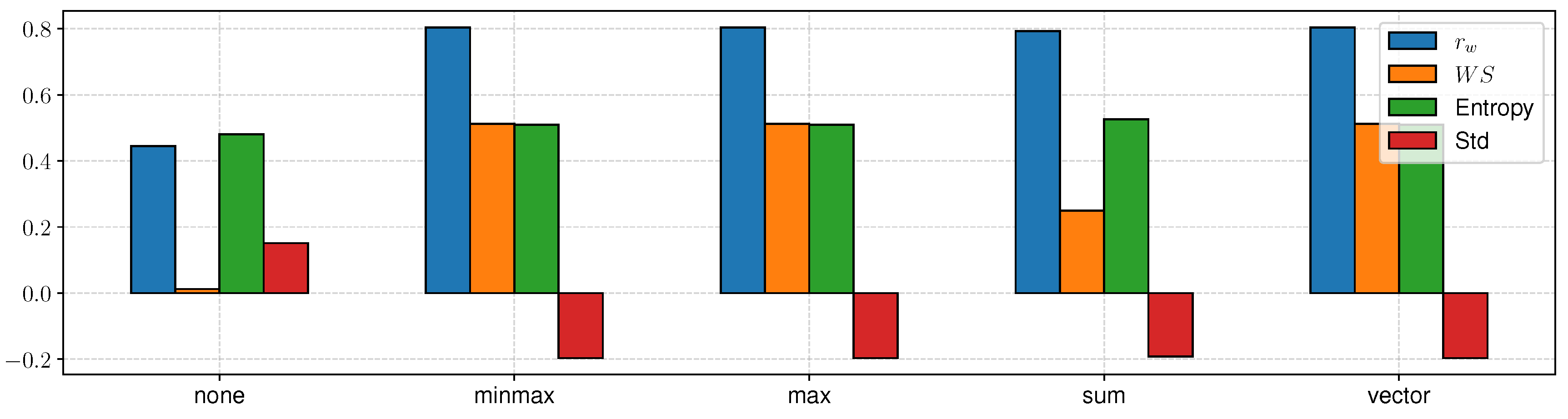
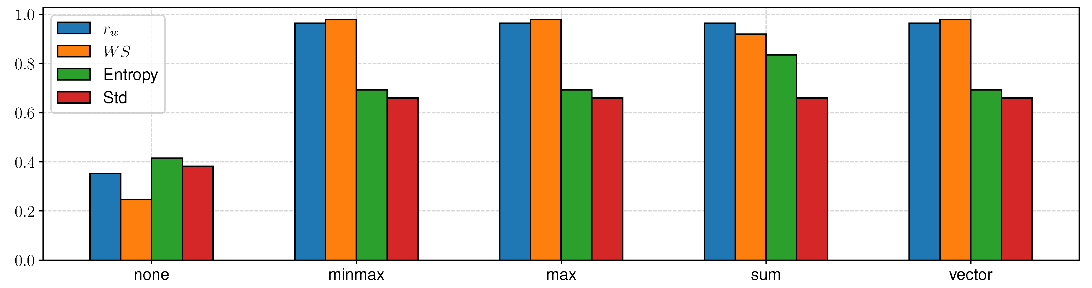
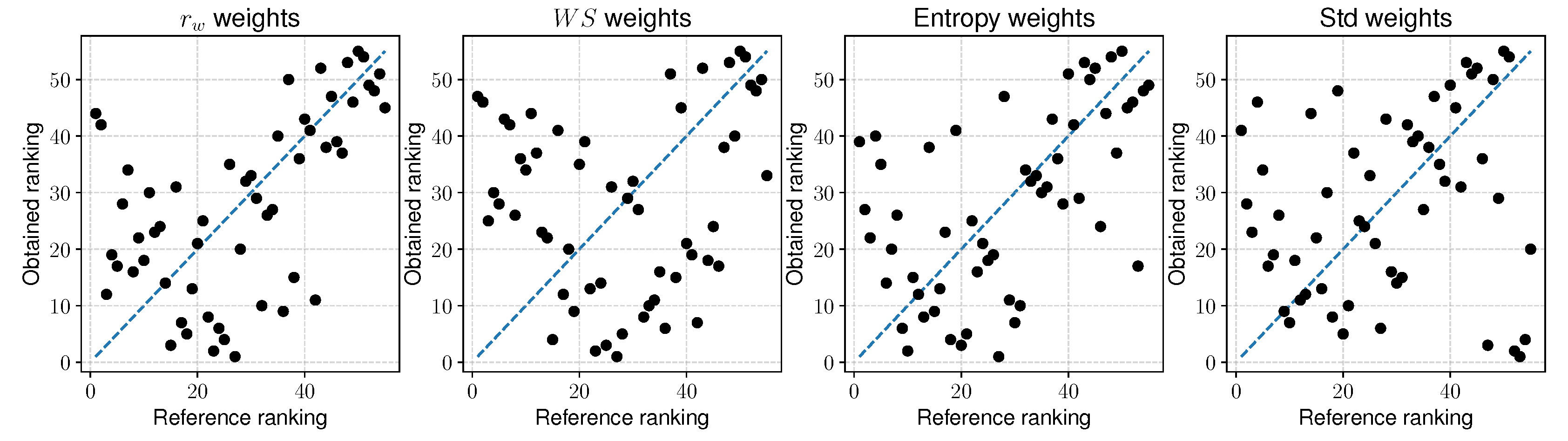
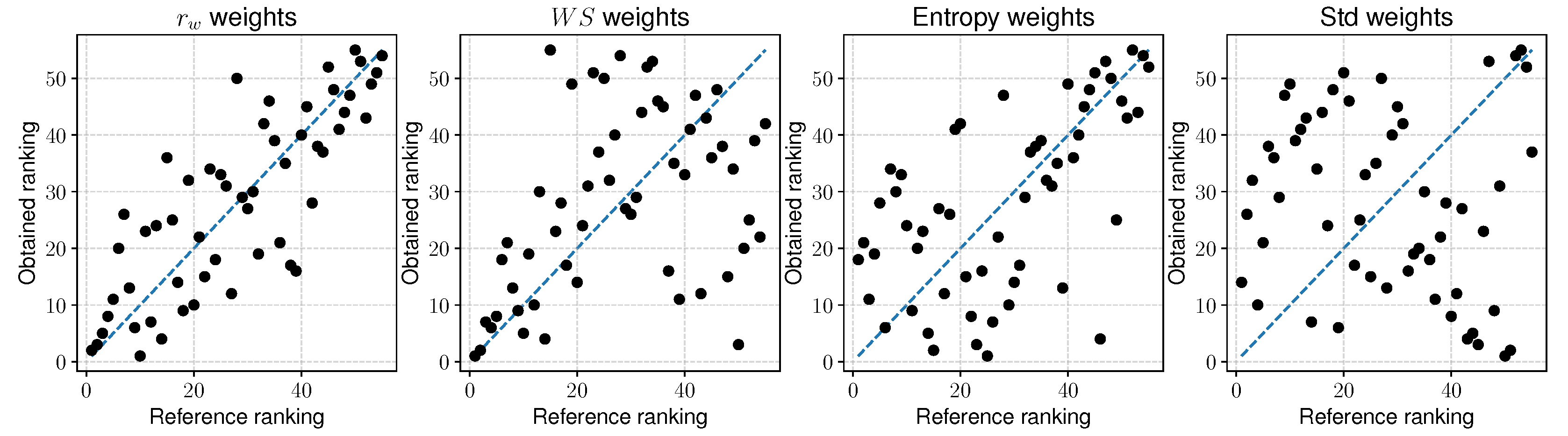
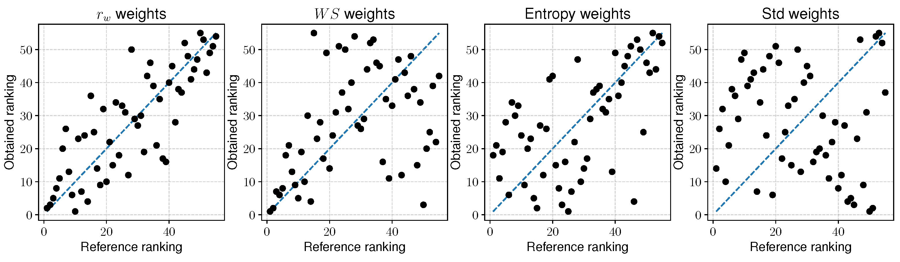
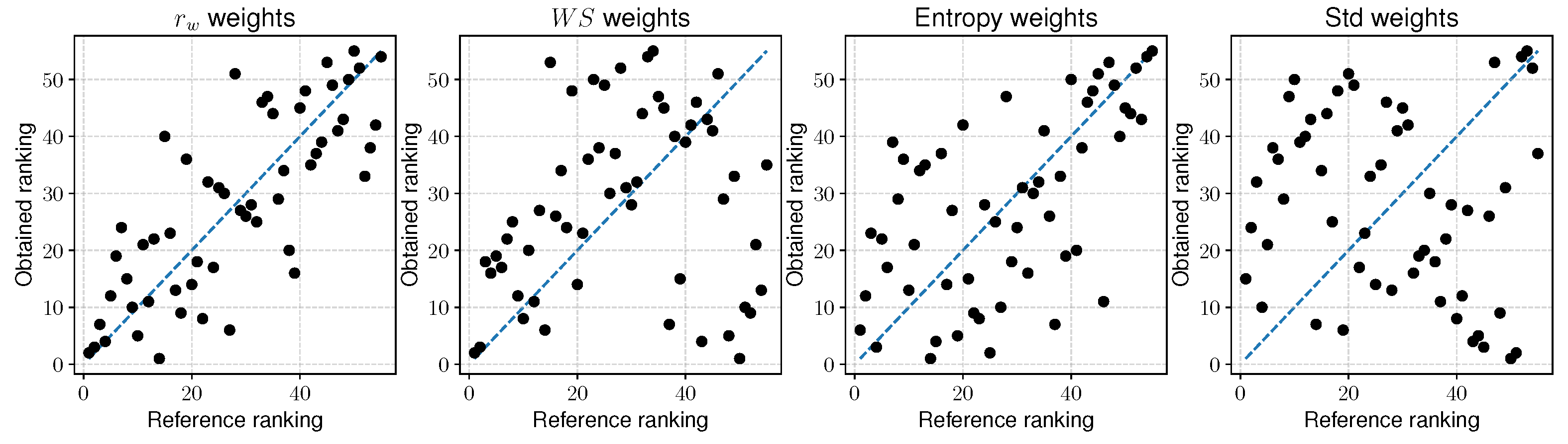
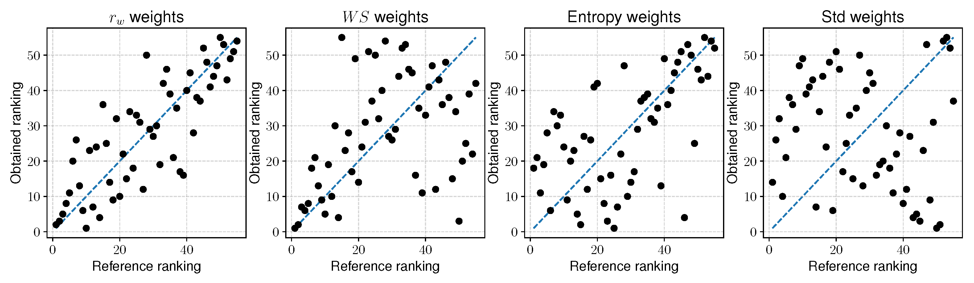
In this work, we present an entirely new approach to determining the relevance of criteria in sustainable transport issues. Based on a comparative study, we analyze the similarity of the approach to determining materiality using $r_w$ and $WS$ as well as standard methods such as entropy and standard deviation. The obtained materiality levels differ significantly. When analyzing which criteria were indicated as the most relevant in the four approaches, it should be pointed out that the most logical ones seem to be those related to the $r_w$ and $WS$. However, in order to empirically verify, an additional study was carried out to check the effectiveness of the calculated criteria weights when using two popular MCDA methods, i.e., TOPSIS and VIKOR. We also examined what the final rankings look like when using different contact normalizations in two cases. We received precise results which indicate that the most effective approach is based on the $r_w$ ratio. At the same time, it is essential to note that the $WS$ ratio approach also has its advantages. Only in one of the nine cases did the entropy method turn out to be the best way to calculate the weighting values. However, it was a case where all the examined methods had poor results. Therefore, based on the conducted research, it can be indicated that the effectiveness of the proposed approaches is higher than the previously used approaches related to entropy and standard deviation.

The limitations of our research are that it concerns one research field, i.e., sustainable transport. Additionally, it should be noted that this is preliminary research which should be extended with extended simulation. Further improvement of approaches related to ranking similarity coefficients should be indicated as the main directions for future work. Further empirical tests related to the use of other methods of determining criterion weighting and other cases of use should be conducted.

References

1. Flamary, R.; Courty, N.; Tuia, D.; Rakotomamonjy, A. Optimal transport for domain adaptation. IEEE Trans. Pattern Anal. Mach. Intell. 2016. [Google Scholar] [CrossRef]
2. Abdul-Manan, A.F. Uncertainty and differences in GHG emissions between electric and conventional gasoline vehicles with implications for transport policy making. Energy Policy 2015, 87, 1–7. [Google Scholar] [CrossRef]
3. Rode, P.; Floater, G.; Thomopoulos, N.; Docherty, J.; Schwinger, P.; Mahendra, A.; Fang, W. Accessibility in Cities: Transport and Urban Form: NCE Cities, Paper 03; LSE: London, UK, 2014. [Google Scholar]
4. Griggs, D.; Stafford-Smith, M.; Gaffney, O.; Rockström, J.; Öhman, M.C.; Shyamsundar, P.; Steffen, W.; Glaser, G.; Kanie, N.; Noble, I. Sustainable development goals for people and planet. Nature 2013, 495, 305–307. [Google Scholar] [CrossRef]
5. Kampa, M.; Castanas, E. Human health effects of air pollution. Environ. Pollut. 2008, 151, 362–367. [Google Scholar] [CrossRef]
6. Landrigan, P.J.; Fuller, R.; Acosta, N.J.; Adeyi, O.; Arnold, R.; Basu, N.N.; Baldé, A.B.; Bertollini, R.; Fuster, V.; Greenstone, M.; et al. The lancet commissions the lancet commission on pollution and health. Lancet 2018, 391, 462–512. [Google Scholar] [CrossRef] [Green Version]
7. Rees, W.; Wackernagel, M. Urban ecological footprints: Why cities cannot be sustainable—And why they are a key to sustainability. In Urban Ecology; Springer: Boston, MA, USA, 2008; pp. 537–555. [Google Scholar]
8. Goldman, T.; Gorham, R. Sustainable urban transport: Four innovative directions. Technol. Soc. 2006, 28, 261–273. [Google Scholar] [CrossRef]
9. Zhao, P. Sustainable urban expansion and transportation in a growing megacity: Consequences of urban sprawl for mobility on the urban fringe of Beijing. Habitat Int. 2010, 34, 236–243. [Google Scholar] [CrossRef]
10. Pojani, D.; Stead, D. Sustainable urban transport in the developing world: Beyond megacities. Sustainability 2015, 7, 7784–7805. [Google Scholar] [CrossRef] [Green Version]
11. De Gruyter, C.; Currie, G.; Rose, G. Sustainability measures of urban public transport in cities: A world review and focus on the Asia/Middle East Region. Sustainability 2017, 9, 43. [Google Scholar] [CrossRef] [Green Version]
12. Hidalgo, D.; Huizenga, C. Implementation of sustainable urban transport in Latin America. Res. Transp. Econ. 2013, 40, 66–77. [Google Scholar] [CrossRef]
13. Mehar, S.; Zeadally, S.; Remy, G.; Senouci, S.M. Sustainable transportation management system for a fleet of electric vehicles. IEEE Trans. Intell. Transp. Syst. 2014, 16, 1401–1414. [Google Scholar] [CrossRef]
14. Banister, D. Unsustainable Transport: City Transport in the New Century; Taylor & Francis: Abingdon, UK, 2005. [Google Scholar]
15. Barfod, M.B.; Salling, K.B. A new composite decision support framework for strategic and sustainable transport appraisals. Transp. Res. Part A: Policy Pract. 2015, 72, 1–15. [Google Scholar] [CrossRef] [Green Version]
16. Pérez, J.C.; Carrillo, M.H.; Montoya-Torres, J.R. Multi-criteria approaches for urban passenger transport systems: A literature review. Ann. Oper. Res. 2015, 226, 69–87. [Google Scholar] [CrossRef]
17. Rajak, S.; Parthiban, P.; Dhanalakshmi, R. Sustainable transportation systems performance evaluation using fuzzy logic. Ecol. Indic. 2016, 71, 503–513. [Google Scholar] [CrossRef]
18. Mukherjee, S. Selection of alternative fuels for sustainable urban transportation under multi-criteria intuitionistic fuzzy environment. Fuzzy Inf. Eng. 2017, 9, 117–135. [Google Scholar] [CrossRef] [Green Version]
19. Mardani, A.; Zavadskas, E.K.; Khalifah, Z.; Jusoh, A.; Nor, K.M. Multiple criteria decision-making techniques in transportation systems: A systematic review of the state of the art literature. Transport 2016, 31, 359–385. [Google Scholar] [CrossRef] [Green Version]
20. Sałabun, W.; Karczmarczyk, A. Using the comet method in the sustainable city transport problem: An empirical study of the electric powered cars. Procedia Comput. Sci. 2018, 126, 2248–2260. [Google Scholar] [CrossRef]
21. Awasthi, A.; Chauhan, S.S. Using AHP and Dempster–Shafer theory for evaluating sustainable transport solutions. Environ. Model. Softw. 2011, 26, 787–796. [Google Scholar] [CrossRef]
22. Aljohani, K.; Thompson, R.G. A stakeholder-based evaluation of the most suitable and sustainable delivery fleet for freight consolidation policies in the inner-city area. Sustainability 2019, 11, 124. [Google Scholar] [CrossRef] [Green Version]
23. Sałabun, W.; Wątróbski, J.; Piegat, A. Identification of a multi-criteria model of location assessment for renewable energy sources. In International Conference on Artificial Intelligence and Soft Computing; Springer: Cham, Switzerland, 2016; pp. 321–332. [Google Scholar]
24. Throne-Holst, H.; Stø, E.; Strandbakken, P. The role of consumption and consumers in zero emission strategies. J. Clean. Prod. 2007, 15, 1328–1336. [Google Scholar] [CrossRef]
25. Wątróbski, J.; Ziemba, P.; Jankowski, J.; Zioło, M. Green energy for a green city—A multi-perspective model approach. Sustainability 2016, 8, 702. [Google Scholar] [CrossRef] [Green Version]
26. Soares, J.; Canizes, B.; Lobo, C.; Vale, Z.; Morais, H. Electric vehicle scenario simulator tool for smart grid operators. Energies 2012, 5, 1881–1899. [Google Scholar] [CrossRef] [Green Version]
27. Ziemba, P. Towards strong sustainability management—A generalized PROSA method. Sustainability 2019, 11, 1555. [Google Scholar] [CrossRef] [Green Version]
28. Ziemba, P.; Wątróbski, J.; Zioło, M.; Karczmarczyk, A. Using the PROSA method in offshore wind farm location problems. Energies 2017, 10, 1755. [Google Scholar] [CrossRef] [Green Version]
29. Wątróbski, J.; Małecki, K.; Kijewska, K.; Iwan, S.; Karczmarczyk, A.; Thompson, R.G. Multi-criteria analysis of electric vans for city logistics. Sustainability 2017, 9, 1453. [Google Scholar] [CrossRef] [Green Version]
30. Sałabun, W.; Karczmarczyk, A.; Wątróbski, J. Decision-making using the hesitant fuzzy sets COMET method: An empirical study of the electric city buses selection. In Proceedings of the 2018 IEEE Symposium Series on Computational Intelligence (SSCI), Bangalore, India, 18–21 November 2018; pp. 1485–1492. [Google Scholar]
31. Ziemba, P. Inter-criteria dependencies-based decision support in the sustainable wind energy management. Energies 2019, 12, 749. [Google Scholar] [CrossRef] [Green Version]
32. De Goes, F.; Breeden, K.; Ostromoukhov, V.; Desbrun, M. Blue noise through optimal transport. ACM Trans. Graph. (TOG) 2012, 31, 1–11. [Google Scholar] [CrossRef]
33. Kontou, E.; Yin, Y.; Lin, Z. Socially optimal electric driving range of plug-in hybrid electric vehicles. Transp. Res. Part D Transp. Environ. 2015, 39, 114–125. [Google Scholar] [CrossRef] [Green Version]
34. Kenworthy, J.R. The eco-city: Ten key transport and planning dimensions for sustainable city development. Environ. Urban. 2006, 18, 67–85. [Google Scholar] [CrossRef]
35. Chen, H.; Jia, B.; Lau, S. Sustainable urban form for Chinese compact cities: Challenges of a rapid urbanized economy. Habitat Int. 2008, 32, 28–40. [Google Scholar] [CrossRef]
36. Suzuki, H.; Cervero, R.; Iuchi, K. Transforming Cities with Transit: Transit and Land-Use Integration for Sustainable Urban Development; The World Bank: Washington, DC, USA, 2013. [Google Scholar]
37. Bagaeen, S. Brand Dubai: The instant city; or the instantly recognizable city. Int. Plan. Stud. 2007, 12, 173–197. [Google Scholar] [CrossRef]
38. Nidumolu, R.; Prahalad, C.K.; Rangaswami, M.R. Why sustainability is now the key driver of innovation. Harv. Bus. Rev. 2009, 87, 56–64. [Google Scholar]
39. Coaffee, J. Risk, resilience, and environmentally sustainable cities. Energy Policy 2008, 36, 4633–4638. [Google Scholar] [CrossRef]
40. Dekker, R.; Bloemhof, J.; Mallidis, I. Operations Research for green logistics–An overview of aspects, issues, contributions and challenges. Eur. J. Oper. Res. 2012, 219, 671–679. [Google Scholar] [CrossRef] [Green Version]
41. Awasthi, A.; Chauhan, S.S. A hybrid approach integrating Affinity Diagram, AHP and fuzzy TOPSIS for sustainable city logistics planning. Appl. Math. Model. 2012, 36, 573–584. [Google Scholar] [CrossRef]
42. Schliwa, G.; Armitage, R.; Aziz, S.; Evans, J.; Rhoades, J. Sustainable city logistics—Making cargo cycles viable for urban freight transport. Res. Transp. Bus. Manag. 2015, 15, 50–57. [Google Scholar] [CrossRef] [Green Version]
43. Crainic, T.G.; Ricciardi, N.; Storchi, G. Models for evaluating and planning city logistics systems. Transp. Sci. 2009, 43, 432–454. [Google Scholar] [CrossRef] [Green Version]
44. Richardson, B.C. Sustainable transport: Analysis frameworks. J. Transp. Geogr. 2005, 13, 29–39. [Google Scholar] [CrossRef]
45. Kelly, C.; May, A.D.; Jopson, A. The development of an option generation tool to identify potential transport policy packages. Transp. Policy 2008, 15, 361–371. [Google Scholar] [CrossRef]
46. Firnkorn, J.; Müller, M. What will be the environmental effects of new free-floating car-sharing systems? The case of car2go in Ulm. Ecol. Econ. 2011, 70, 1519–1528. [Google Scholar] [CrossRef]
47. Firnkorn, J.; Müller, M. Selling mobility instead of cars: New business strategies of automakers and the impact on private vehicle holding. Bus. Strategy Environ. 2012, 21, 264–280. [Google Scholar] [CrossRef]
48. Ampudia-Renuncio, M.; Guirao, B.; Molina-Sanchez, R. The impact of free-floating carsharing on sustainable cities: Analysis of first experiences in Madrid with the university campus. Sustain. Cities Soc. 2018, 43, 462–475. [Google Scholar] [CrossRef]
49. Kopp, J.; Gerike, R.; Axhausen, K.W. Do sharing people behave differently? An empirical evaluation of the distinctive mobility patterns of free-floating car-sharing members. Transportation 2015, 42, 449–469. [Google Scholar] [CrossRef]
50. Lehmann, S. Green urbanism: Formulating a Series of Holistic Principles. Available online: http://journals.openedition.org/sapiens/1057 (accessed on 10 June 2020).
51. Cherry, C.R.; Weinert, J.X.; Xinmiao, Y. Comparative environmental impacts of electric bikes in China. Transp. Res. Part D Transp. Environ. 2009, 14, 281–290. [Google Scholar] [CrossRef] [Green Version]
52. Buehler, R.; Pucher, J.; Gerike, R.; Götschi, T. Reducing car dependence in the heart of Europe: Lessons from Germany, Austria, and Switzerland. Transp. Rev. 2017, 37, 4–28. [Google Scholar] [CrossRef]
53. Offer, G.J.; Contestabile, M.; Howey, D.; Clague, R.; Brandon, N.P. Techno-economic and behavioural analysis of battery electric, hydrogen fuel cell and hybrid vehicles in a future sustainable road transport system in the UK. Energy Policy 2011, 39, 1939–1950. [Google Scholar] [CrossRef] [Green Version]
54. Sałabun, W.; Palczewski, K.; Wątróbski, J. Multicriteria approach to sustainable transport evaluation under incomplete knowledge: Electric bikes case study. Sustainability 2019, 11, 3314. [Google Scholar] [CrossRef] [Green Version]
55. Zadeh, L. Fuzzy sets. Inf. Control 1965, 8, 338–353. [Google Scholar] [CrossRef] [Green Version]
56. Piegat, A.; Sałabun, W. Comparative analysis of MCDM methods for assessing the severity of chronic liver disease. In International Conference on Artificial Intelligence and Soft Computing; Springer: Cham, Switzerland, 2015; pp. 228–238. [Google Scholar]
57. Jankowski, J.; Sałabun, W.; Wątróbski, J. Identification of a multi-criteria assessment model of relation between editorial and commercial content in web systems. In Multimedia and Network Information Systems; Springer: Cham, Switzerland, 2017; pp. 295–305. [Google Scholar]
58. Salabun, W.; Napierala, M.; Bykowski, J. The Identification of Multi-Criteria Model of the Signicficance of Drainage Pumping Stations in Poland. Acta Sci. Polonorum. Form. Circumiectus 2015, 14, 147. [Google Scholar] [CrossRef]
59. Faizi, S.; Sałabun, W.; Rashid, T.; Wątróbski, J.; Zafar, S. Group decision-making for hesitant fuzzy sets based on characteristic objects method. Symmetry 2017, 9, 136. [Google Scholar] [CrossRef]
60. Faizi, S.; Rashid, T.; Sałabun, W.; Zafar, S.; Wątróbski, J. Decision making with uncertainty using hesitant fuzzy sets. Int. J. Fuzzy Syst. 2018, 20, 93–103. [Google Scholar] [CrossRef] [Green Version]
61. Sałabun, W. Reduction in the number of comparisons required to create matrix of expert judgment in the comet method. Manag. Prod. Eng. Rev. 2014, 5, 62–69. [Google Scholar] [CrossRef]
62. Sałabun, W.; Karczmarczyk, A.; Wątróbski, J.; Jankowski, J. Handling Data Uncertainty in Decision Making with COMET. In Proceedings of the 2018 IEEE Symposium Series on Computational Intelligence (SSCI), Bangalore, India, 18–21 November 2018; pp. 1478–1484. [Google Scholar]
63. Wątróbski, J.; Jankowski, J.; Ziemba, P.; Karczmarczyk, A.; Zioło, M. Generalised framework for multi-criteria method selection. Omega 2019, 86, 107–124. [Google Scholar] [CrossRef]
64. Faizi, S.; Sałabun, W.; Ullah, S.; Rashid, T.; Więckowski, J. A New Method to Support Decision-Making in an Uncertain Environment Based on Normalized Interval-Valued Triangular Fuzzy Numbers and COMET Technique. Symmetry 2020, 12, 516. [Google Scholar] [CrossRef] [Green Version]
65. Sałabun, W. The Characteristic Objects Method: A New Distance-based Approach to Multicriteria Decision-making Problems. J. Multi-Criteria Decis. Anal. 2015, 22, 37–50. [Google Scholar] [CrossRef]
66. Behzadian, M.; Otaghsara, S.K.; Yazdani, M.; Ignatius, J. A state-of the-art survey of TOPSIS applications. Expert Syst. Appl. 2012, 39, 13051–13069. [Google Scholar] [CrossRef]
67. Sałabun, W. The mean error estimation of TOPSIS method using a fuzzy reference models. J. Theor. Appl. Comput. Sci. 2013, 7, 40–50. [Google Scholar]
68. Opricovic, S. Multicriteria optimization of civil engineering systems. Fac. Civ. Eng. Belgrade 1998, 2, 5–21. [Google Scholar]
69. Opricovic, S.; Tzeng, G.H. Compromise solution by MCDM methods: A comparative analysis of VIKOR and TOPSIS. Eur. J. Oper. Res. 2004, 156, 445–456. [Google Scholar] [CrossRef]
70. Papathanasiou, J.; Ploskas, N. Multiple Criteria Decision Aid; Springer: Cham, Switzerland, 2018. [Google Scholar]
71. Sałabun, W.; Urbaniak, K. A new coefficient of rankings similarity in decision-making problems. In International Conference on Computational Science; Springer: Cham, Switzerland, 2020. [Google Scholar]
72. Podviezko, A. Distortions introduced by normalisation of values of criteria in multiple criteria methods of evaluation. LMD Darb 2014, 55, 51–56. [Google Scholar] [CrossRef]
73. Zardari, N.H.; Ahmed, K.; Shirazi, S.M.; Yusop, Z.B. Weighting Methods and Their Effects on Multi-Criteria Decision Making Model Outcomes in Water Resources Management; Springer: Cham, Switzerland, 2015. [Google Scholar]
Figure 1. The research procedure.
Sustainability 12 07915 g001
Figure 2. The procedure of the COMET method.
Sustainability 12 07915 g002
Figure 3. Visualization of linguistic values, i.e., low—blue, medium—orange and high—green, for criteria C 1 C 8 .
Sustainability 12 07915 g003
Figure 4. Visualization of the similarity of the reference ranking and eight derived rankings.
Sustainability 12 07915 g004
Figure 5. Visualize the relevance of criteria using different methods.
Sustainability 12 07915 g005
Figure 6. Comparison of the results from the reference ranking and the ranking obtained by using TOPSIS—minmax.
Sustainability 12 07915 g006
Figure 7. Comparison of the results from the reference ranking and the ranking obtained by using TOPSIS—max.
Sustainability 12 07915 g007
Figure 8. Comparison of the results from the reference ranking and the ranking obtained by using TOPSIS—sum.
Sustainability 12 07915 g008
Figure 9. Comparison of the results from the reference ranking and the ranking obtained by using TOPSIS—vector.
Sustainability 12 07915 g009
Figure 10. Visualization of the results from the reference ranking and the ranking obtained by using TOPSIS and different normalization techniques ( r w coefficient).
Sustainability 12 07915 g010
Figure 11. Visualization of the results from the reference ranking and the ranking obtained by using TOPSIS and different normalization techniques ( W S coefficient).
Sustainability 12 07915 g011
Figure 12. Visualization of the results from the reference ranking and the ranking obtained by using VIKOR and different normalization techniques ( r w coefficient).
Sustainability 12 07915 g012
Figure 13. Visualization of the results from the reference ranking and the ranking obtained by using VIKOR and different normalization techniques ( W S coefficient).
Sustainability 12 07915 g013