Article

Monitoring and Mathematical Modeling of Soil and Groundwater Contamination by Harmful Emissions of Nitrogen Dioxide from Motor Vehicles

1
Department of Computer Science, West Ukrainian National University, 11 Lvivs’ka Str., 46000 Ternopil, Ukraine
2
Department of Information Systems, Wroclaw University of Economics and Business, Komandorska 118/120, 53-345 Wroclaw, Poland
*
Authors to whom correspondence should be addressed.
Sustainability 2021, 13(5), 2768; https://0-doi-org.brum.beds.ac.uk/10.3390/su13052768
Submission received: 4 January 2021 / Revised: 26 February 2021 / Accepted: 28 February 2021 / Published: 4 March 2021
(This article belongs to the Special Issue Methods, Tools, Indexes and Frameworks in Sustainability Assessment)

Abstract

:
The article considers the task and a new approach to monitoring of soil and groundwater contamination by harmful emissions of nitrogen dioxide from motor vehicles. The approach is based on combination of measurement procedure of the harmful emissions concentrations in the surface atmospheric layer and mathematical modeling of the impact of these emissions on soil and groundwater contamination. The scheme of this harmful emission concentrations measurement using a mobile complex Sniffer4D Hyper-local Air Quality Analyzer is given. Based on these results, a mathematical model of diffusion of this harmful substance in the upper layers of soil and water resources is proposed. As a result of the computations, the distribution of concentrations of soil and water contamination in the neighborhood of separate observation points has been built. Also, the field of nitrogen dioxide concentrations at various depths for observation points has been modeled. For a waterbody, the concentration of nitric acid, which is formed due to the interaction of nitrogen dioxide with water, is higher in water than in the surface layer of the soil. This concentration can be significantly increased during prolonged downpours when acidic solutions drain from surrounding soil areas into the waterbodies. The obtained research results are fully consistent with the practical and theoretical results on the diffusion of gases into soils and water resources. It means that the proposed approach can be used instead of the existing very expensive approach to analysis of soil and groundwater contamination in the laboratory.

1. Introduction

Environmental contamination due to human anthropogenic activities is one of the greatest challenges facing humanity that requires implementation of regulatory policy [1]. Pollutants lead to negative changes in flora and fauna. Also, directly or indirectly contribute to the deterioration of human health causing various diseases and pathologies [2]. The nature of contamination sources is different. Respectively, their complex impact on air, soil and water resources is different [3]. In order to reduce the negative impact on the environment, there are variety of systems for its monitoring [4]. The best results have been achieved in the monitoring of atmospheric air, the quality of which has a direct impact on the human respiratory system and mainly leads to immediate consequences for the disease [5]. At the same time, special attention needs to be paid to the identification and research of the condition of particularly dangerous sources of soil and groundwater contamination [1,6,7,8,9]. Their contamination mainly have more prolonged negative consequences for human health, as well as for flora and fauna, compared to air pollution [10,11].
It should be noted that a large number of tools are available to monitor air contamination [12]. Such systems are deployed both to control pollution by motor vehicles in large cities [12], and to monitor air contamination by other objects such as chemical plants and thermal and nuclear power plants [13]. There are also a huge number of sensors for operational air quality analysis, or for checking of contaminants or pollutants presence in the air. However, for the soil and groundwater contamination, such the operational monitoring is significantly complicated [14,15,16]. Mainly, the monitoring of soils and groundwater is based on the technologies of analysis of soil and groundwater contamination involve the collection of soil or groundwater samples at different depths with their subsequent analysis in the laboratory [6,14,15,16,17,18,19]. This approach to monitoring is not operational and expensive [14,19]. However, with this approach it is very difficult to establish the origin of contamination, i.e., their sources.
As known [20,21,22], the main sources of chemical contamination of soil are chemical substances used in agriculture (fertilizers, pesticides, etc.), precipitation within the range of industrial enterprises (especially, chemical and metallurgical ones), mining, thermal and nuclear power plants, and also, motor vehicles.
Chemical contamination of soil due to the absorption of harmful substances by the top layer of soil is relevant for large cities, as well as for the surrounding soils and waterbodies. It should be noted that the research of soil contamination through atmospheric air is considered in [23,24]. At the same time, insufficient attention is paid to the monitoring of this type of soil and water contamination. Indirect soil contamination due to precipitation is mainly considered [24,25]. However, they do not take into account, for example, contamination of soils and waterbodies by harmful emissions in the exhaust gases of motor vehicles. In such cases, due to high humidity, diffusion processes and close proximity of the emission sources to the soil and waterbodies, this type of contamination causes pollution of soils, groundwater and adjacent waterbodies [18,26].
It should be noted that there is a range of harmful substances in the motor vehicles exhaust gases. Nitrogen dioxide in high concentrations is the most dangerous of them [27,28]. The problem about nitrogen dioxide consists in emission to atmospheric surface layer, which contributes to the direct diffusion of this contaminant into the soil and waterbodies surrounding the road sections. Further processes of nitrogen dioxide diffusion related to entering to groundwater, transforming into nitric acid and leaching of its salts into waterbodies. It causes the saturation of waterbodies with nitrates which are known to be extremely harmful for humans and fauna [29]. For large cities, such contamination is critical compared to other types. For example, this type of contamination is more than 50% for large cities [30]. Because, contamination sources of nitrogen dioxide or other harmful substances from thermal power plants or other chemical plants are mainly at a great distance from the surface layer and this fact contributes to the partial dispersion and transfer of contaminants to other places over long distances, outside the surrounding areas, where they settle on the ground or into waterbodies in lower concentrations [31].
Thus, we can state that the existing approaches to the analysis of soil and groundwater contamination, which involve the sampling of soil or groundwater with their subsequent analysis in the laboratory, are inefficient and expensive. Especially when it comes to such type of contamination as harmful emissions in the exhaust gases of motor vehicles [14,15,16,19]. At the same time, organization of monitoring of air contamination by harmful emissions in the exhaust gases of motor vehicles is practically solved problem for the majority of economically developed countries [12,27,28,29,32]. Based on the above, a complex approach to solving of problem of monitoring of soil and groundwater contamination due to harmful emissions in the exhaust gases of motor vehicles is proposed. The essence of the approach consists in combination of procedure of measurement of harmful emissions concentration in the surface atmospheric layer and mathematical modeling of the impact of these emissions on soil and groundwater contamination.
A separate question is modeling and predicting of the consequences of soil and groundwater contamination due to the absorption of gaseous substances by the soil. For these purposes, mathematical models are used in the form of differential equations in partial derivatives, or their difference analogues which are synthesized by algorithms of structural identification [4,5,27]. Such mathematical models are sufficiently studied and considered in a large number of scientific papers. At the same time, for their building, it is necessary to set the initial conditions. It again leads to the use of a certain number of soil samples from some upper layer and laboratory studies of collected samples to establish concentrations of contaminants [6,9,19,25]. However, the problem of “initial conditions” for mathematical model building can be solved within the above-announced complex approach.
For these purposes, it is necessary to use a system for monitoring of contamination by motor vehicles of the surface atmospheric layer [27,28,32]. Based on the above, the task of monitoring of soil and groundwater contamination by harmful nitrogen dioxide emissions from vehicles by the using approach of combining means of measurement concentration of this harmful emissions in the surface atmospheric layer and mathematical modeling of the impact of these emissions on soil and groundwater contamination is represented in this article.

2. Materials and Methods

2.1. Mathematical Models of Nitrogen Dioxide Diffusion in Soil and Waterbody

As it was mentioned earlier, the main task of the research is to monitor the surface atmospheric layer in order to detect the contamination by nitrogen dioxide, followed by modeling of absorption of this contamination into the soil. The measurements of the contaminants concentration in the surface atmospheric layer (almost on the soil surface) make it possible to research the processes of penetration of these contaminants into the soil and waterbodies. From this surface, gaseous contaminants penetrate into the upper layers of loose soil.
In a humid environment, nitrogen dioxide reacts with water according to the reaction [33]:
2 NO 2 + H 2 O HNO 3 + HNO 2
In its turn, nitric acid, which is formed during the absorption of nitrogen dioxide, as unstable compound decomposes into nitrogen oxide and nitric acid [33]:
3 HNO 2 HNO 3 + 2 NO + H 2 O
As a result, we can consider the reaction:
6 NO 2 + 3 H 2 O 4 HNO 3 + 2 NO + H 2 O  
Reducing both parts of the equation by molecule of water, we obtain the basic equation of formation of nitric acid:
3 NO 2 + H 2 O 2 HNO 3 + NO
Nitric acid in aqueous solutions dissociates into ions. As a strong monobasic acid, it interacts with basic and amphoteric oxides (of copper and zinc), with bases, and displaces weak acids from their salts. For example, calcium carbonate, which is found in limestone and chalk. Nitrogen dioxide and nitric acid are toxic substances. The maximum permissible concentrations of which C NO 2 B , C HNO 3 B are limited by national standards. Significant exceed of the maximum allowable doses is the basis for chemical reclamation of soils with limestone fertilizers and construction of treatment facilities for waterbodies.
The main mechanism of mass transfer of gases in the soil and gas exchange between the soil and the atmosphere is diffusion—the movement of gases under the action of a concentration gradient. Convective (under the action of temperature gradients), gravitational (under the action of gravity) mechanisms and also, mechanism under the action of atmospheric pressure differences are of auxiliary nature [34].
The approaches to modeling of nitrogen dioxide concentration in the soil have been analyzed. The analyzed areas of contaminations are characterized by a fairly large size compared to the depth of penetration of contamination. The contamination concentration on the soil surface is not characterized by significant gradients. It allows to consider the analysis of the concentrations field of contamination in the soil as a local problem at each observation point on the surface with a single argument which is the distance of the observation point from the soil surface. In this case, a one-dimensional diffusion equation is obtained:
d d h [ D S ( h ) d C i S ( h ) d h ] =   0 ,
where i is the observation point number, D S ( h ) is the coefficient of diffusion of nitrogen dioxide in the soil, and C i S ( h ) is the concentration of soil contamination in the neighborhood of i-th observation point.
The nonlinear differential diffusion Equation (5) is given in the form convenient for application of numerical methods:
d 2 C i S ( h ) d h 2 + D S ( h ) D S ( h ) d C i S ( h ) d h = 0
It has been complemented with the Dirichlet boundary conditions on the soil surface (h = 0), where the observation results Pi of surface contamination at the i-th observation point, adjusted for the difference between the values of diffusion coefficients in air D A   and on the soil surface D S ( 0 ) have been used:
C i S ( 0 ) = P i D S ( 0 ) D A
At the lower bound of the most fertile soil layer Hy in the first approximation, we apply the Neumann-type no-slip condition:
d C i S ( h ) d h | h = H y = 0
It should be noted that there is a problem of determination of the diffusion coefficient distribution in the soil. To determine it, it is necessary to take such factors into account: soil type, atmospheric conditions, such as daily and seasonal changes of air temperature and atmospheric pressure, temperature gradients at the air-soil surface boundary, atmospheric air turbulence, precipitation and nature of their distribution, intensity and volume of water evaporation [35]. Based on the theoretical background [34,35], it can be stated that all these parameters will only affect the diffusion coefficient distribution. The basic diffusion model in this case remains unchanged. If it is possible to investigate the diffusion coefficient distribution for specific conditions, it could easily be taken into account in the proposed model. However, the modeling of the diffusion coefficient distribution itself is a separate task that goes beyond the scope of this research.
An analogue task can be set for a waterbody. Assuming that the diffusion coefficient in water is constant, we can obtain an analytical representation of its solution. But, the assumption of the constancy of the diffusion coefficient of nitric acid in water is, in our opinion, an oversimplification. In particular, according to the resource [35], such a diffusion coefficient depends on the concentration of the acid itself. Given this, the one-dimensional equation of diffusion of nitric acid in water:
d d h [ D W ( C i W ( h ) ) d C i W ( h ) d h ]   =   0
is given in the following way:
D W ( C i W ( h ) ) C i W [ d C i W ( h ) d h ] 2 + D W ( C i W ( h ) ) d 2 C i W ( h ) d h 2 = 0  
By analogy with modeling problem represented by Equations (6)–(8), we obtain the modeling problem represented by Equations (11)–(13) for building of distribution of nitric acid concentration in the water:
d 2 C i W ( h ) d h 2 + D W ( C i W ( h ) ) C i W D W ( C i W ( h ) ) [ d C i W ( h ) d h ] 2 = 0
C i W ( 0 ) = P i W
d C i W ( h ) d h | h = H b = 0
where i is the observation point number, D W ( C ) is the function of nitric acid diffusion in the water depending on its concentration, C i W ( h ) is concentration of water contamination in the neighborhood of i-th observation point and H b is averaged depth of waterbody.
To solve the Equations (6)–(8) and (11)–(13), the software module solve_bvp from “integrate” section of Python library Scipy has been used. The module is based on the “shooting method” using the method of difference approximations, which is described in [36].
The use of this module involves the representation of the functional dependence of NO2 diffusion coefficient in the soil. To build it, the data from the source [37] have been used as well as the UnivariateSpline module from the “interpolate” section of the Python library Scipy.

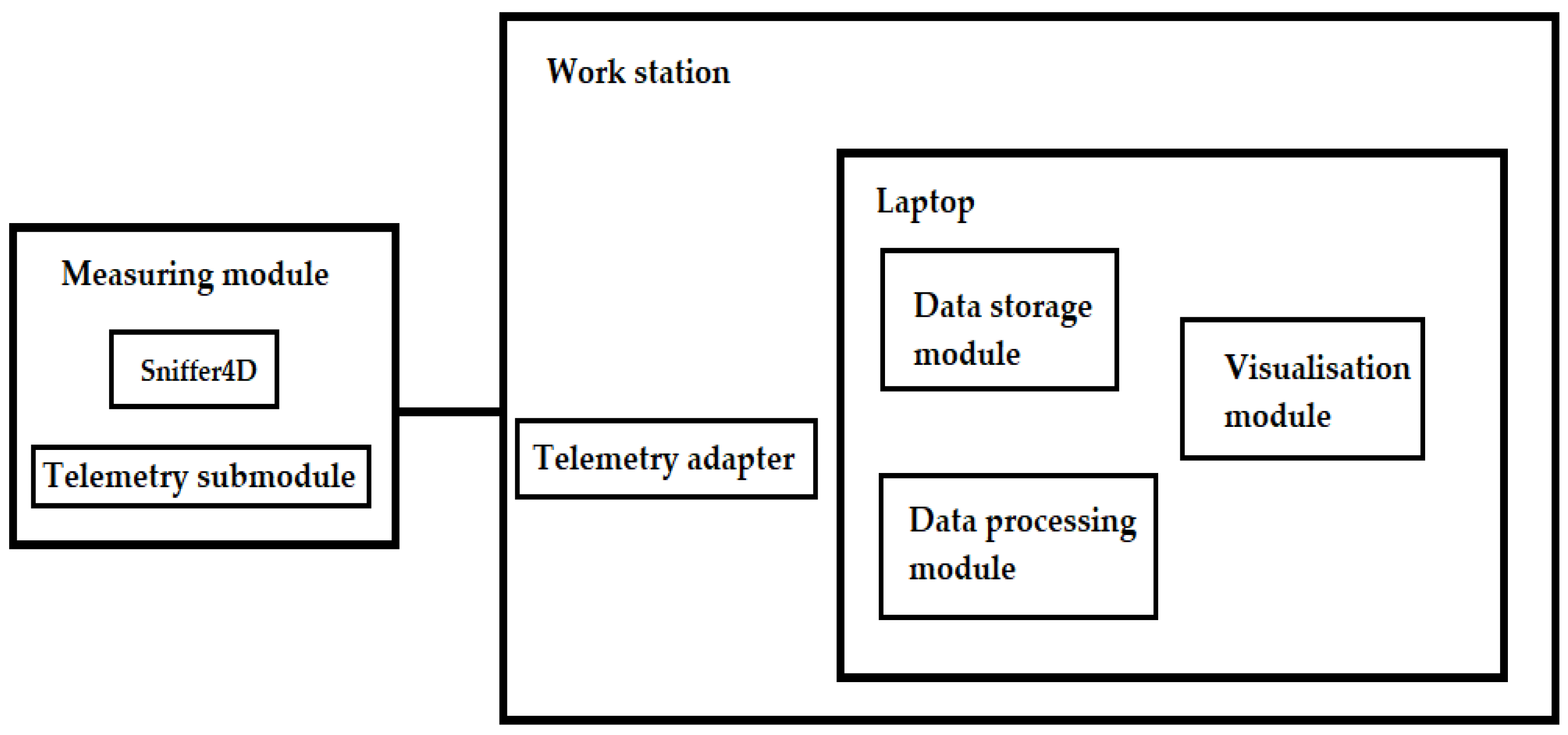
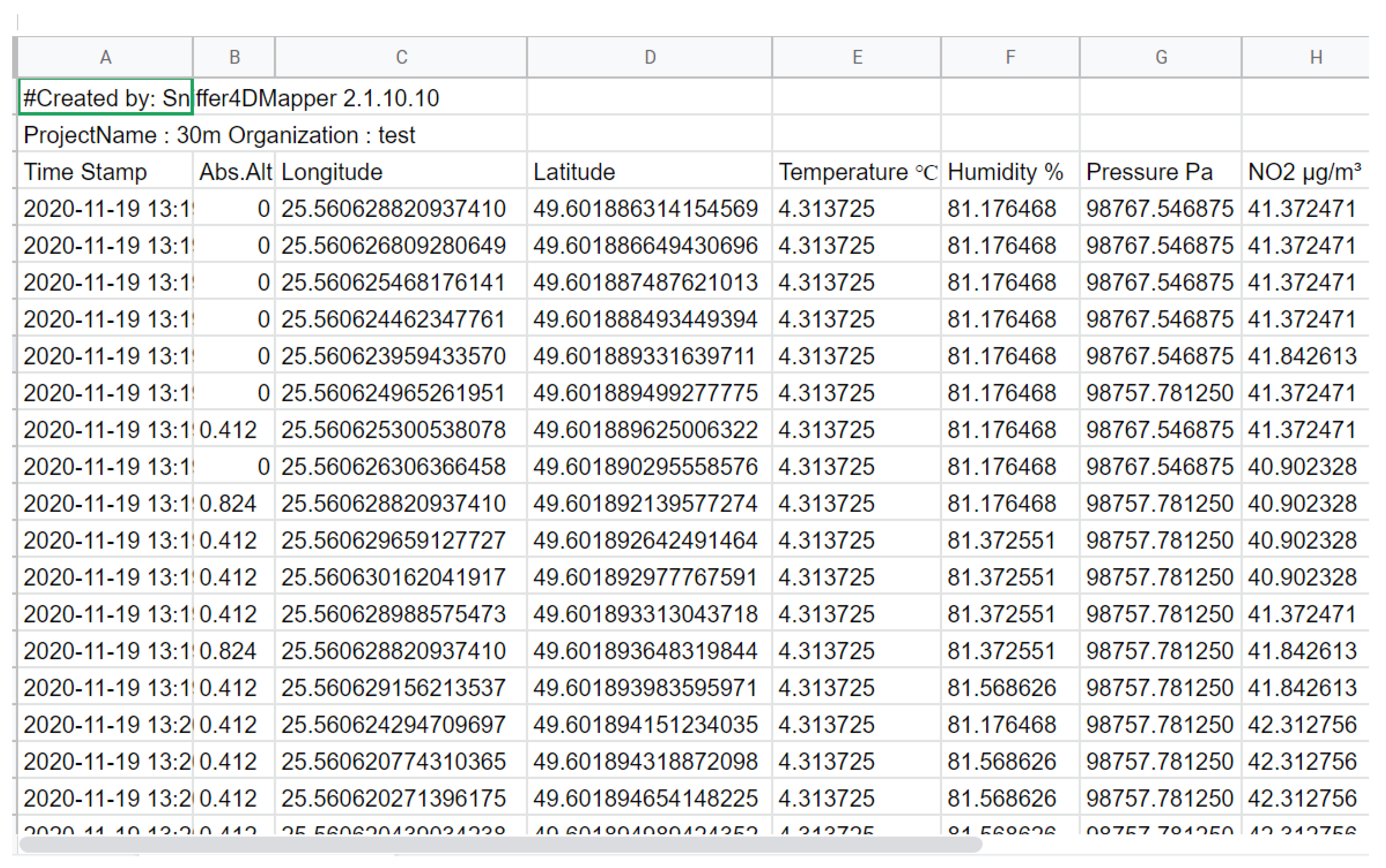
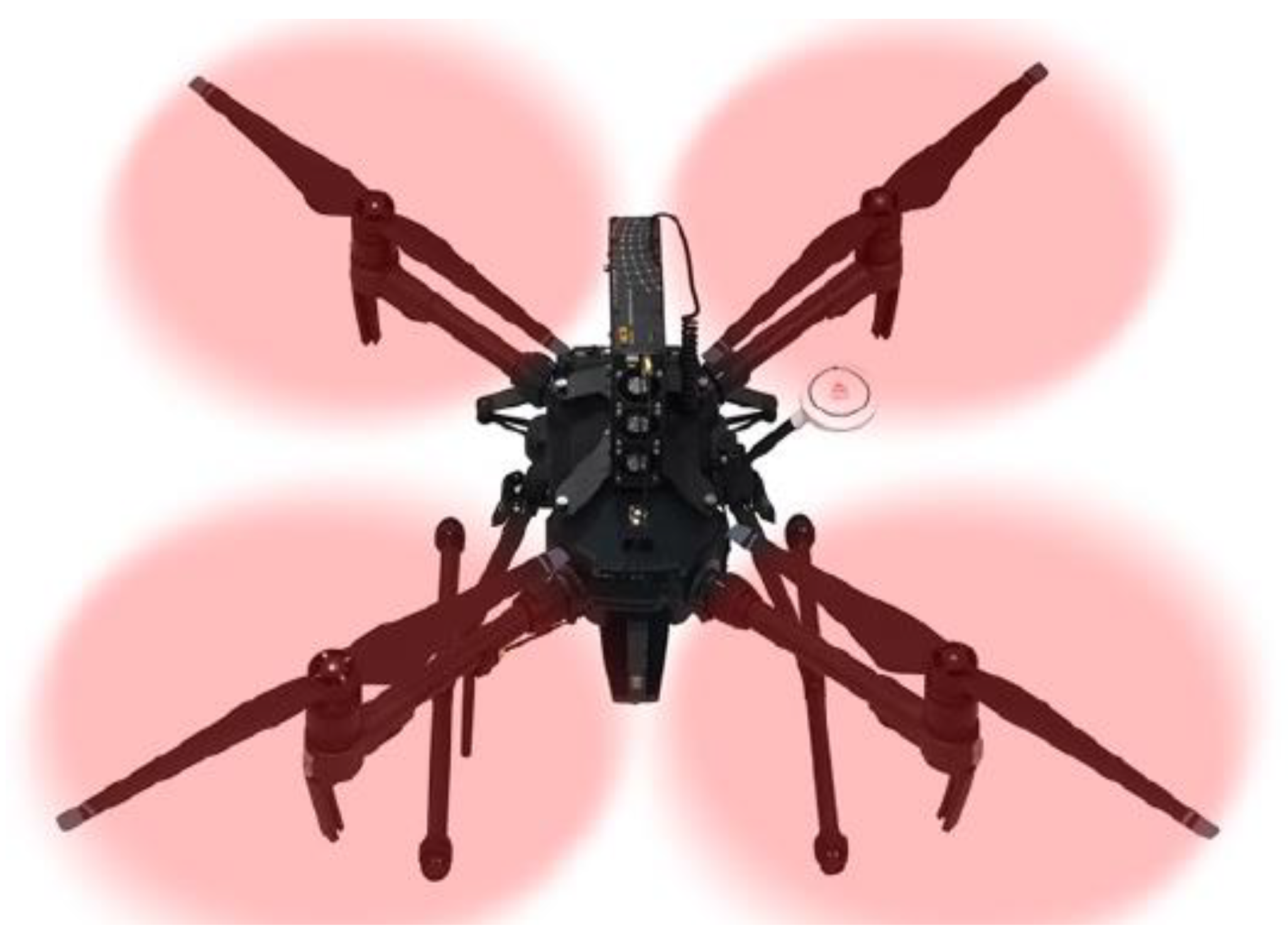
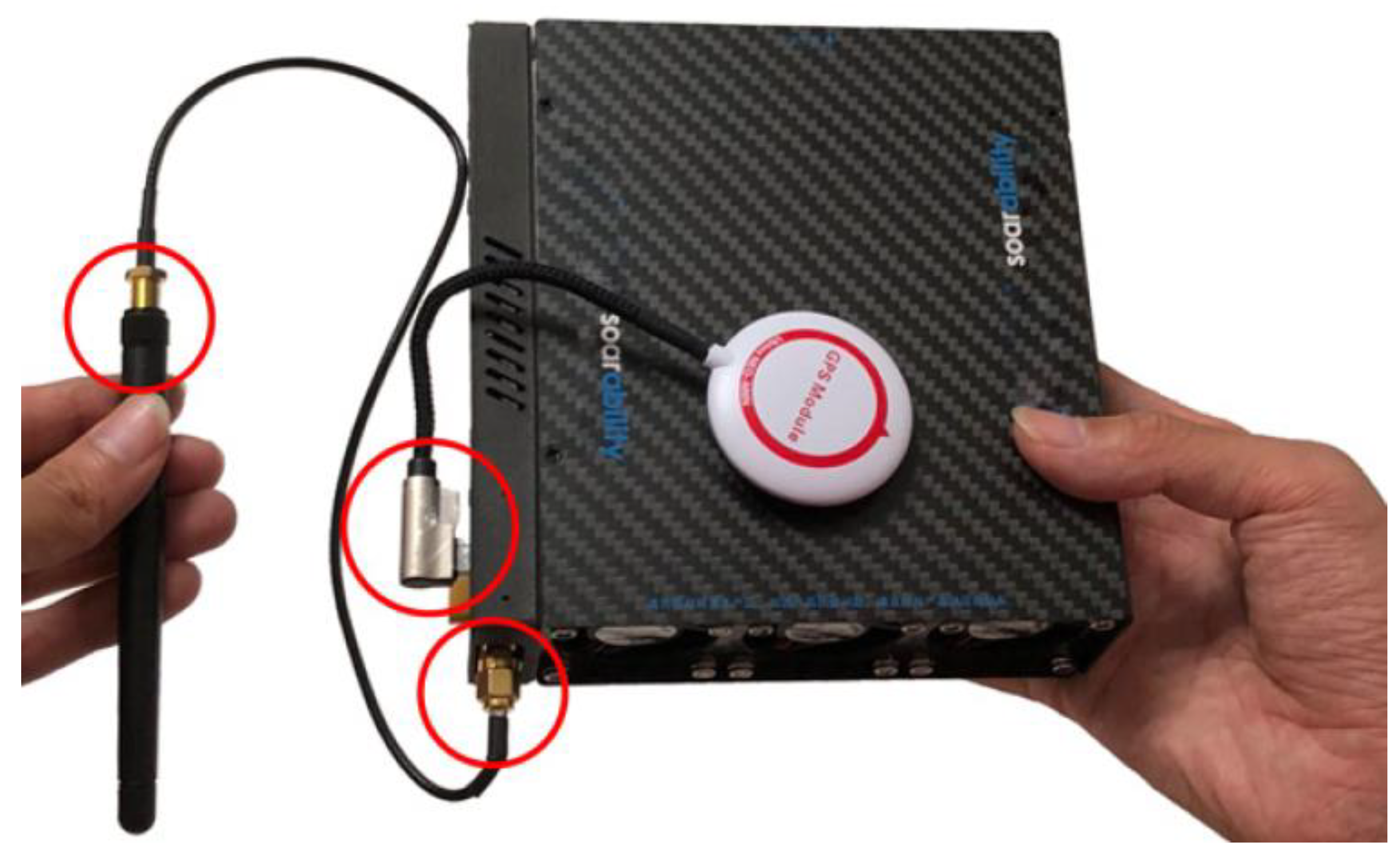
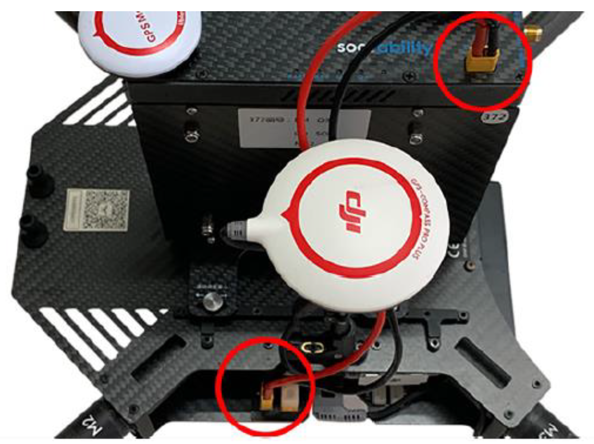
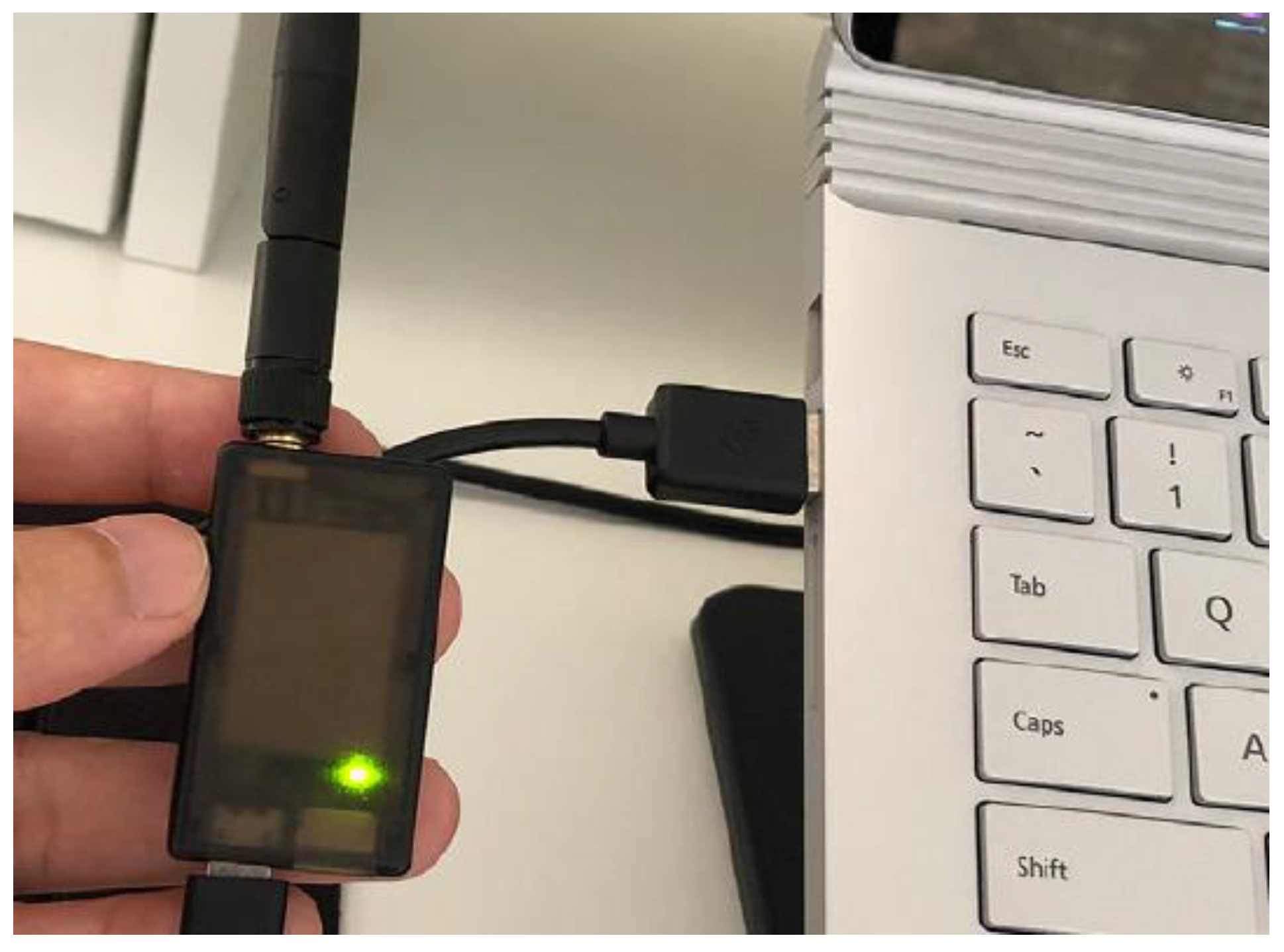
2.2. Monitoring Tools

Based on the previous work of the authors [32], the basic element to monitor the nitrogen dioxide concentration is the Sniffer4D Hyper-local Air Quality Analyzer unit [38], with the nitrogen dioxide measuring sensor installed. The general view of Sniffer4D Hyper-local Air Quality Analyzer sensors is presented in Appendix A (Figure A1).
One of the main advantage of this sensor unit is the presence of automated calibration system, together with other advantages: high measurement accuracy; wide range of operating temperatures; instant response time and significant service life. This unit is installed onboard the DJI M100 quadcopter mobile system [39] as shown in Appendix A (Figure A2).
To organize the data transmission between the mobile system and the base station, where the measurement results are stored, it is necessary to do some settings of the Sniffer4D unit. First of all, there is a need to connect the GPS module to the main unit using a micro USB connector and a telemetry antenna to the antenna port of the device using an extension cord. General view of device with connected stuff is represent in the Appendix A (Figure A3).
The result of installation of the Sniffer4D unit onto the quadcopter is showed in the Appendix A (Figure A4). In particular, fixation of unit, connection of the unit’s power supply via the XT30U port to the main power supply of the quadcopter.
To transmit the data between the Sniffer4D Hyper-local Air Quality Analyzer unit and the base station, Sniffer4D Mapper software is installed on the personal computer of this station. It allows not only to pre-process the telemetry data and record them into the database, but also to visualize and analyze the results of real-time measurements. Also, after installing the specified software, the unit sensor and the Sniffer4D Mapper utility have been synchronized. To do this, the telemetry module (receiver) united with the device, is connected to the computer, as shown in the Appendix A (Figure A5), the specified software module is launched.
Broad overview of the Sniffer4D Mapper interface is shown in the Appendix A (Figure A6). As we can see, the synchronization ensures transmission and visual representation of telemetry results (contaminants concentrations, environment temperature, atmospheric pressure and humidity) on the background of the area map where these telemetry data are collected.
Data from the Sniffer4D Hyper-local Air Quality Analyzer sensor are transmitted in real time via the telemetry module and antennas to the base station and entered into the Sniffer4D Mapper software. Schematically, the architecture of the monitoring system is shown in Figure 1.
As can be seen from the above Figure 1, the monitoring system consists of two main parts. The first part is a measuring module (consisting of Sniffer4D, which is installed on a quadcopter and a telemetry submodule for data transmission). The second part is a workstation built on the basis of a computer to which a telemetry adapter is connected to receive the data from the measuring module via radio channel. Data is transmitted between modules over TCP/IP, which is excellent for quick exchange of large information amount. Next, the software part of the monitoring system is considered in more detail. The received data is stored in a file, what the data storage module is responsible for. Further information processing is performed in the data processing module. The main business logic of this module is based on the developed mathematical diffusion model. The computations results are visualized on the background of the area map.

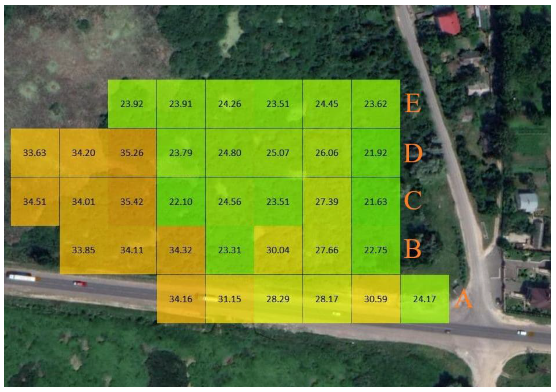
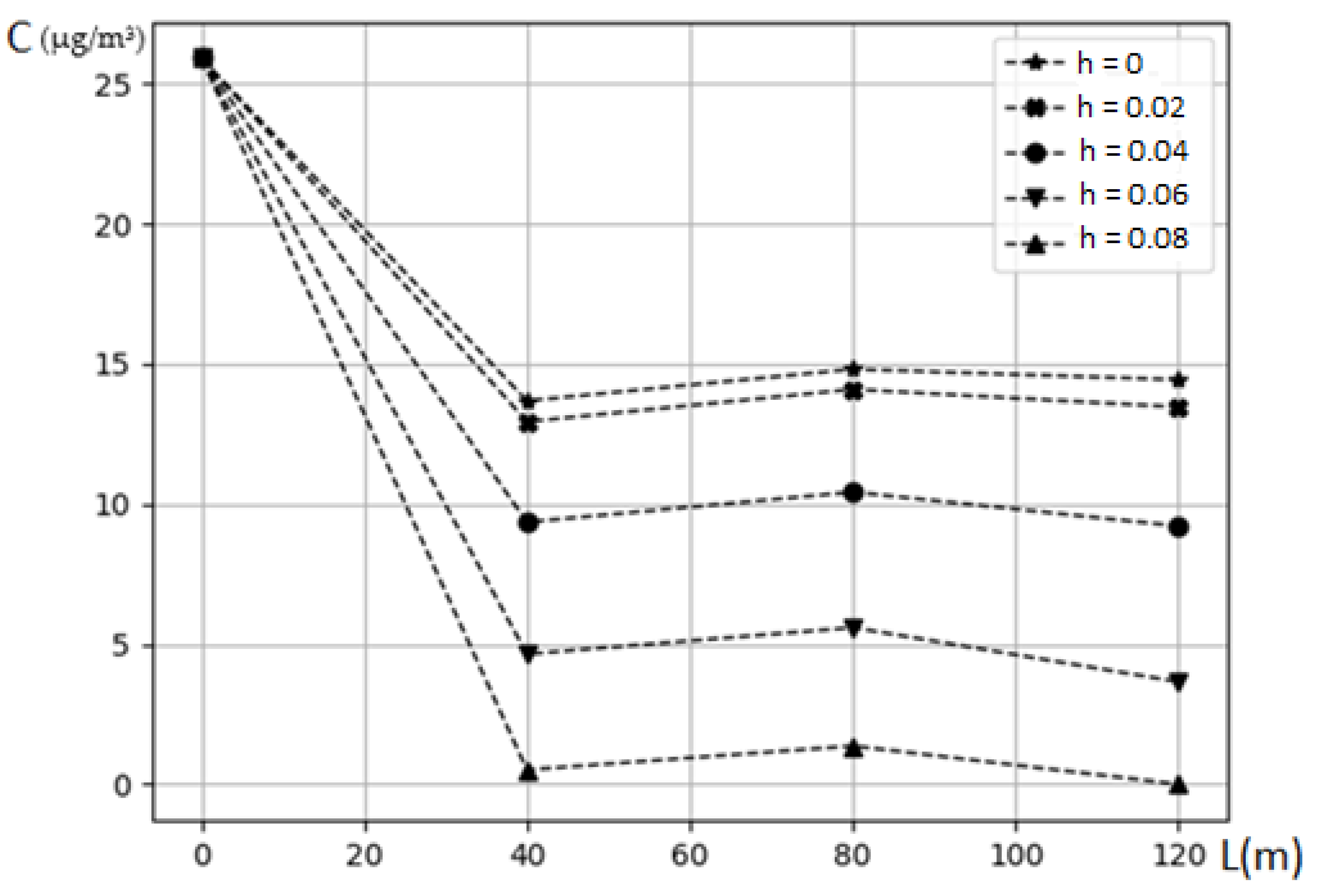
3. Results and Discussion

The assessment of impact of nitrogen dioxide on soil contamination has been executed on the section of the road P41 at a distance of up to 200 m. This section is characterized by heavy traffic and is located on a highway of regional importance in Ukraine, near the village of Chistyliv (a bypass road in Ternopil, Ukraine).
Initially, the measurements have been executed at a height of 1–5 m (atmospheric surface layer) above the road and along the road at a distance of 2–5 m.
In the course of research of the mentioned road section, the instant values of the ni-trogen dioxide concentration have been measured, which have been further used to calcu-late the initial conditions required to solve the differential diffusion Equation (6). The type of soil at the research location is black soil. The characteristics of it, to calculate the diffusion coefficient distribution, are given in the work [37]. Other conditions for calculation of values the diffusion coefficient distribution have been selected from the Table 1.
The measurement results are shown in the Figure 2A,B. By moving the aircraft (quadcopter) with the Sniffer4D Hyper-local Air Quality Analyzer complex, the following measurements, in the same way, have been executed along the road at a distance of 10–30 m, Figure 2C, 40–70 m, Figure 2D, 70–90 m, Figure 2E, 100–130 m, Figure 2F, 140–160 m, Figure 2G.
In the second series of the research, the aircraft complex measured nitrogen dioxide concentrations at a height of 30 m above the same road section. Measurements at this height are necessary to assess how the concentration of nitrogen dioxide varies depending on distance from the ground. In a similar way, as in the first experiment, the measurements have been executed along the road above the road: Figure 3A, at a distance of 10–30 m from the road, Figure 3B, 40–70 m, Figure 3C, 70–90 m, Figure 3D, 100–130 m, Figure 3E.
The instantaneous values of nitrogen dioxide concentration in micrograms per cubic meter of air ( 10 6 g m 3 ) have been recorded on the obtained “square” plots.
As can be seen from Figure 2, the concentration of nitrogen dioxide in the atmospheric surface layer for the selected area ranges from 37.61   × 10 6 g m 3 to 44.21   × 10 6 g m 3 . At this, it is higher near the road and decreases at bigger distances from the road. From Figure 2, it can be concluded that with increasing of distance from the soil surface, the concentration decreases. It should be noted that at height of about 100 m in this area, the concentration of nitrogen dioxide has decreased by at least 10 times compared to the concentration in the surface layer. From the above, the assumption can be made that the contamination source is harmful emissions of nitrogen dioxide in the exhaust gases of motor vehicles moving on the road. Using the installed software Sniffer4D Mapper, a data table is prepared. The fragment of the data table is shown in the form of the Figure 4.
The table shows the time of measurements, the coordinates of the points where the measurements were made, the conditions of measurements (temperature, atmospheric pressure and humidity of the air), as well as the concentrations of nitrogen dioxide at the measurement points. Using the data table generated by the software Sniffer4D Mapper, part of the data have been selected from it to illustrate the proposed mathematical model. The selected data have been presented in the Table 1 of nitrogen dioxide measurement results.
The results of some numerical experiments implemented on the basis of the described method are demonstrated below. Observations from line D (Figure 1) have been selected for demonstration and entered into the Table 1 of nitrogen dioxide measurement results. Table 1 shows 10 observation points. Each of them is characterized by the time, the meteorological conditions of the measurements and the measured concentrations of nitrogen dioxide. Instead of the points spatial coordinates (as illustrated in Figure 4), Table 1 shows the distances from the left edge of the line (D or G) to each of the observation points.
They are characterized by relatively significant differences in the observed contamination concentrations. In the first series of experiments, the distribution of soil contamination concentrations in the neighborhood of points of line D has been modeled, where the largest, the smallest, and median values of contamination concentrations in the surface atmospheric layer have been observed. The results of the experiments are presented in the Figure 5. It should be noted that the initial values of concentrations in the upper soil layer are recalculated relative to the concentrations in the atmosphere, according to equation (7). The abscissa axis represents the distance (depth) from the soil surface in meters, and the ordinate axis shows the contamination concentrations with a factor of 10 6 g m 3 . Analysis of the graphs shows that significant penetration of contaminants in the gaseous state stops almost at a depth of 0.1 m. This result, from the point of view of process physics, is qualitatively completely consistent with the results of gas diffusion in soils [37].
In the next series of experiments, the contamination concentrations have been modeled in the neighborhood of each observation point of line D. The corresponding concentrations at different depths up to 0.1 m are shown in the Figure 6. The abscissa axis shows the distances of observation points from the left edge of line D, and the ordinate axis shows the contamination concentrations with a factor of 10 6 g m 3 . The uniform decrease in concentration at all points of line D has been observed.
The modeling problem represented by Equations (11)–(13) has been analyzed. First of all, the diffusion coefficients of nitrogen dioxide in air and water have been compared. According to the publication [40], at the lowest acid concentrations, the diffusion coefficient is 2.984 · 10 1 m 2 s .
This is 104 times more than the diffusion coefficient of nitrogen dioxide in the air. Such a significant predominance of the diffusion coefficient in water over the diffusion coefficient in air leads to the fact that the contamination concentration in the upper layer of water will be equal to the concentration in the other layers of water. Minimal changes in the diffusion coefficient of nitric acid in a wide range of its concentration mean that the second component in Equation (11) can be equated to zero. The zero Neumann condition in the lower layer of water means that this concentration is constant throughout the layer. Therefore, it remains to accept the assumption that concentration of nitric acid is constant at the level of the bound value:
P i W = 2 3 P i
The coefficient is obtained from the equation of chemical reaction (4) according to the principle of mass conservation.
The conducted analysis together with the solving method of modeling problem represented by Equations (6)–(8) allows building of contamination distribution along the line G (Figure 2), which crosses both the surface of the waterbody and the soil. Data for modeling at four points along the line G are shown in the Table 1. The results of the corresponding numerical experiments are represented in the Figure 7. It is worth to note that the first point of the line G in the Table 1 (distance is 0 m) is located above the lake surface.
The abscissa axis shows the distances of the observation points from the left edge of the line G, and the ordinate axis shows the concentrations of contamination with the factor 10 6 g m 3 . At the same time, the concentration of contamination in a waterbody significantly exceeds the soil contamination concentration. This result is qualitatively consistent with the results of the physics of gas diffusion in water and soil [34,35,37].
As a result of the executed computations, the distribution of contamination concentrations for soil and water in the neighborhood of individual observation points has been built, as well as the distribution of contamination concentration in the neighborhood of the pair of observation points of waterbody-coast subsystem.

4. Conclusions

The considered problem of soil and groundwater contamination monitoring, as well as mathematical models of the contaminants distribution are relevant for large cities with adjacent agricultural lands and water resources. One of the most dangerous harmful substance in the exhaust gases of motor vehicles is the nitrogen dioxide. The main results of the research have been established with the help of the mobile information and measuring complex Sniffer4D Hyper-local Air Quality Analyzer and mathematical models of nitrogen dioxide diffusion in the upper soil layers and water resources. The proposed approach to monitoring is based on combination of procedure of measurement of harmful emissions concentration in the surface atmospheric layer and mathematical modeling of the impact of these emissions on soil and groundwater contamination.
As a result of the executed computations, the distribution of contamination concentration for soil and water in the neighborhood of individual observation points is built, as well as the distribution of contamination concentration in the neighborhood of a pair of observation points of waterbody-coast subsystem. In the first series of experiments, the contamination concentrations distribution in the cross section of the soil in the neighborhood of the points along the line has been modeled based on the obtained concentrations from the mobile measuring complex where the largest, smallest and median values of contamination concentrations in the surface layer have been observed.
It has been established that significant penetration of contaminants in the gaseous state stop almost at a depth of 0.1 m.
In the next series of experiments, the contamination concentrations have been modeled in the neighborhood of each observation point along one line. A uniform decrease of concentration in all points of the line with increase of the depth has been observed, which is fully consistent with the physics of the diffusion process. For a waterbody, the diffusion coefficients are significantly higher and, accordingly, the concentration of nitric acid, which is formed due to the interaction of nitrogen dioxide with water, is higher in water than in the surface layer of the soil.
Numerical experiments indicate the highest concentration of contamination caused by nitrogen dioxide in waterbodies. This concentration can significantly increase during prolonged downpours when acidic solutions drain from the surrounding soil areas into waterbodies. The obtained research results are fully consistent with the practical and theoretical results on the diffusion of gases into soils and water resources obtained by other authors [34,35,37]. It means that the proposed approach can be used instead of the existing very expensive approach to analysis of soil, groundwater and waterbodies contamination in a laboratory.

Author Contributions

Conceptualization, M.D. and A.R.; methodology, R.P.; software, V.T. and N.H.; validation, R.P. and A.R.; formal analysis, M.D. and R.P.; investigation, M.D and V.T.; resources, M.D and A.R.; data curation, V.T. and N.H.; writing—original draft preparation, M.D. and Y.M.; writing—review and editing, M.D and Y.M.; visualization, V.T.; supervision, M.D. and A.R.; project administration, M.D. and A.R.; funding acquisition, A.R. All authors have read and agreed to the published version of the manuscript.

Funding

The research is supported by the Ministry of Science and Higher Education in Poland under the programme “Regional Initiative of Excellence” 2019–2022 project number 015/RID/2018/19 total funding amount 10 721 040,00 PLN and partially supported by the Ministry of Education and Science of Ukraine under the grant “Mathematical tools and software for identification and monitoring of particularly dangerous sources of soil and groundwater pollution” January 2020–December 2021, state registration number 0120U102040.

Institutional Review Board Statement

Not applicable.

Informed Consent Statement

Not applicable.

Data Availability Statement

Data is contained within the article.

Conflicts of Interest

The authors declare no conflict of interest.

Appendix A

Figure A1. General view of Sniffer4D Hyper-local Air Quality Analyzer sensors [38].
Sustainability 13 02768 g0a1
Figure A2. Integration of Sniffer4D unit with DJI M100 quadcopter [39].
Sustainability 13 02768 g0a2
Figure A3. Connection of telemetry antenna and GPS module to the Sniffer4D unit [39].
Sustainability 13 02768 g0a3
Figure A4. Installation of Sniffer4D unit onto quadcopter [39].
Sustainability 13 02768 g0a4
Figure A5. Telemetry module connected to the computer [39].
Sustainability 13 02768 g0a5
Figure A6. A general overview of the software interface of Sniffer4D Mapper with the synchronized sensor.
Sustainability 13 02768 g0a6

References

  1. Rausch, A. CMS Guide on Soil and Groundwater Contamination; CMS.Low.Tax.: Kyiv, Ukraine, 2019; p. 54. Available online: https://cms.law/en/media/international/files/publications/guides/soil-and-groundwater-contamination-guide (accessed on 17 November 2020).
  2. Stefurak, V.P.; Yastrebova, O.S. Environment and human health. Galician Med. Bull. 2014, 1, 126–128. [Google Scholar]
  3. Vasyukova, T.G. Ecology: A Textbook; Concord: Kyiv, Ukraine, 2012; 524p. [Google Scholar]
  4. Dyvak, M.; Porplytsya, N.; Maslyiak, Y.; Kasatkina, N. Modified artificial bee colony algorithm for structure identification of models of objects with distributed parameters and control. In Proceedings of the 2017 14th International Conference, The Experience of Designing and Application of CAD Systems in Microelectronics (CADSM), Lviv, Ukraine, 21–25 February 2017; pp. 50–54. [Google Scholar] [CrossRef]
  5. Porplytsya, N.; Dyvak, M. Interval difference operator for the task of identification recurrent laryngeal nerve. In Proceedings of the 2015 16th International Conference on Computational Problems of Electrical Engineering (CPEE), Lviv, Ukraine, 2–5 September 2015; pp. 156–158. [Google Scholar] [CrossRef]
  6. Amin Al Manmi, D.A.M.; Abdullah, T.O.; Al-Jaf, P.M.; Al-Ansari, N. Soil and Groundwater Pollution Assessment and Delineation of Intensity Risk Map in Sulaymaniyah City, NE of Iraq. Water 2019, 11, 2158. [Google Scholar] [CrossRef] [Green Version]
  7. La Cecilia, D.; Porta, G.M.; Tang, F.H.; Riva, M.; Maggi, F. Probabilistic indicators for soil and groundwater contamination risk assessment. Ecol. Indic. 2020, 115, 106424. [Google Scholar] [CrossRef]
  8. Moranda, A.; Cianci, R.; Paladino, O. Analytical Solutions of One-Dimensional Contaminant Transport in Soils with Source Production-Decay. Soil Syst. 2018, 2, 40. [Google Scholar] [CrossRef] [Green Version]
  9. Hoghooghi, N.; Radcliffe, D.E.; Habteselassie, M.Y.; Clarke, J.S. Confirmation of the Impact of Onsite Wastewater Treatment Systems on Stream Base-Flow Nitrogen Concentrations in Urban Watersheds of Metropolitan Atlanta, GA. J. Environ. Qual. 2016, 45, 1740–1748. [Google Scholar] [CrossRef]
  10. Kotsur, N.I. Environmental risks and human health: Current problems and solutions. Young Sci. 2016, 9.1, 91–94. [Google Scholar]
  11. Ugochukwu, U.C.; Ochonogor, A. Groundwater contamination by polycyclic aromatic hydrocarbon due to diesel spill from a telecom base station in a Nigerian City: Assessment of human health risk exposure. Environ. Monit. Assess 2018, 190, 249. [Google Scholar] [CrossRef] [PubMed]
  12. Smit, R.; Kingston, P. Measuring On-Road Vehicle Emissions with Multiple Instruments Including Remote Sensing. Atmosphere 2019, 10, 516. [Google Scholar] [CrossRef] [Green Version]
  13. Dragomir, E.G.; Oprea, M. A Multi-Agent System for Power Plants Air Pollution Monitoring. IFAC Proc. Vol. 2013, 46, 89–94. [Google Scholar] [CrossRef]
  14. Bottomley, P.J.; Angle, J.S.; Weaver, R.W. Part 2: Microbiological and Biochemical Properties. In Methods of Soil Analysis, 1st ed.; Soil Science Society of America: Madison, WI, USA, 2011. [Google Scholar]
  15. Zhao, L.; Hu, Y.M.; Zhou, W.; Liu, Z.H.; Pan, Y.C.; Shi, Z.; Wang, L.; Wang, G.X. Estimation Methods for Soil Mercury Content Using Hyperspectral Remote Sensing. Sustainability 2018, 10, 2474. [Google Scholar] [CrossRef] [Green Version]
  16. Sparks, D.L.; Bartels, J.M. Methods of Soil Analysis: Chemical Methods. Part 3; John Wiley & Sons: Hoboken, NJ, USA, 2020; p. 1424. [Google Scholar]
  17. De Corato, U. Towards New Soil Management Strategies for Improving Soil Quality and Ecosystem Services in Sustainable Agriculture: Editorial Overview. Sustainability 2020, 12, 9398. [Google Scholar] [CrossRef]
  18. Nawrot, N.; Wojciechowska, E.; Rezania, S.; Walkusz-Miotk, J.; Pazdro, K. The effects of urban vehicle traffic on heavy metal contamination in road sweeping waste and bottom sediments of retention tanks. Sci. Total Environ. 2020, 749, 141511. [Google Scholar] [CrossRef] [PubMed]
  19. Koda, E.; Osinski, P.; Sieczka, A.; Wychowaniak, D. Areal Distribution of Ammonium Contamination of Soil-Water Environment in the Vicinity of Old Municipal Landfill Site with Vertical Barrier. Water 2015, 7, 2656–2672. [Google Scholar] [CrossRef]
  20. Baliuk, S.; Medvedev, V.; Miroshnichenko, M.; Skrylnik, Y.; Timchenko, D.; Fatieev, A.; Khristenko, A.; Tsapko, Y. Environmental State of Soils in Ukraine; National Scientific Center; Institute for Soil Science and Agrochemistry Research: Kharkiv, Ukraine, 2015; pp. 38–42. [Google Scholar]
  21. Matviychuk, V.K.; Khar, I.O. Monograph. In Atmospheric Air Pollution; National Academy of Management: Kyiv, Ukraine, 2013; 272p. [Google Scholar]
  22. Popova, A.O. Sources of land pollution by hazardous substances and their sorts. In Current Problems of the State and Law; Collection of Scientific Works: Kyiv, Ukraine, 2014; Volume 73, pp. 443–450. Available online: http://nbuv.gov.ua/UJRN/apdp_2014_73_73 (accessed on 17 November 2020).
  23. Yurchenko, V.A.; Mikhailova, L.S.; Bespalova, M.V. Investigation of the influence of the road on the ecosystems of the roadside space. In Bulletin of the Kharkiv National Automobile University: A Collection of Scientific Papers; Kharkiv National Automobile and Road University: Kharkiv, Ukraine, 2018; pp. 29–32. [Google Scholar]
  24. Melnikova, O.G.; Yurchenko, V.A. Ecological consequences of technogenic load created by road-infrastructure complexes on soil ecosystems. In Proceedings of the IX International Scientific and Practical Conference. Ecological, Legal and Economic Aspects of Ecological Security of the Regions, Kharkiv, Ukraine, 29–31 October 2014; pp. 232–236. Available online: https://dspace.khadi.kharkov.ua/dspace/bitstream/123456789/966/1/24_64.pdf (accessed on 16 November 2020).
  25. Paul, S.; Cashman, M.A.; Szura, K.; Pradhanang, S.M. Assessment of Nitrogen Inputs into Hunt River by Onsite Wastewater Treatment Systems via SWAT Simulation. Water 2017, 9, 610. [Google Scholar] [CrossRef] [Green Version]
  26. Dzhigirey, V.S. Ecology and Protection of the Natural Environment, 3rd ed.; KOO: Znannya, Ukraine, 2014; 309p. [Google Scholar]
  27. Ocheretnyuk, N.; Voytyuk, I.; Dyvak, M.; Martsenyuk, Y. Features of structure identification the macromodels for nonstationary fields of air pollutions from vehicles. In Proceedings of the Modern Problems of Radio Engineering, Telecommunications and Computer Science—Proceedings of the 11th International Conference, Lviv, Ukraine, 17–19 May 2012; p. 444. [Google Scholar]
  28. Dyvak, M.; Porplytsya, N.; Borivets, I.; Shynkaryk, M. Improving the computational implementation of the parametric identification method for interval discrete dynamic models. In Proceedings of the 2017 12th International Scientific and Technical Conference on Computer Sciences and Information Technologies (CSIT), Lviv, Ukraine, 5–8 September 2017; pp. 533–536. [Google Scholar] [CrossRef]
  29. Bilyavsky, G.O.; Butchenko, L.I.; Navrotsky, V.M. Fundamentals of Ecology: Theory and Workshop; Book-K.: Kyiv, Ukraine, 2012; 352p. [Google Scholar]
  30. Sukharev, S.M.; Chundak, S.Y.; Sukhareva, O.Y. Technology and Environmental Protection: Textbook; New World: Lviv, Ukraine, 2014; 252p. [Google Scholar]
  31. Filina, T.V. Change in the activity of some soil enzymes under the influence of metals. Biol. Ser. Ecol. 1999, 4, 114–118. [Google Scholar]
  32. Dyvak, M.P.; Masliyak, Y.B.; Pukas, A.V.; Porplytsya, N.P.; Voitiuk, I.F.; Tymchyshyn, V.S. Architecture of the ecological monitoring system and an example of its application for modeling concentrations of harmful emissions from motor transport. Ind. Model. Complex Syst. 2017, 9, 69–84. [Google Scholar]
  33. Zakharov, I.I.; Lishchyshyna, T.P.; Zakharova, O.I. Ecologically pure technology for the nitric acid reproduction. Visnyk East. Ukr. Natl. Univ. Volodymyr Dahl 2014, 9, 7–14. [Google Scholar]
  34. Pozniak, S.P. Soil Science and Geography of Soils; Ivan Franko Lviv National University: Lviv, Ukraine, 2010; 270p. [Google Scholar]
  35. Diffusion Coefficient of Aqueous Solutions in Pure Water. Available online: http://weldworld.ru/theory/summary/koefficient-diffuzii-vodnyh-rastvorov-v-chistoy-vode.html (accessed on 18 November 2020).
  36. Clark, K.D.; Petzold, L.R. Numerical solution of boundary value problems in differential-algebraic systems. SIAM J. Sci. Stat. Comput. 2009, 10, 915–938. [Google Scholar] [CrossRef] [Green Version]
  37. Kovdy, V.A.; Rozanov, B.G. Soil Science; Higher School: Moscow, Russia, 1988; 400p. [Google Scholar]
  38. Image. Available online: http://sniffer4d.eu/ (accessed on 16 November 2020).
  39. Image. Available online: https://newwezhanoss.oss-cn-hangzhou.aliyuncs.com/contents/sitefiles2012/10062246/files/157744.pdf?Expires=1608257644&OSSAccessKeyId=LTAIekGM1705vEQp&Signature=DLFXu%2BZ0v9686mMRSuiI7rCrUQc%3D&response-content-disposition=inline%3Bfilename%3DEn_Sniffer4D_User_Manual_191109.pdf&response-content-type=application%2Fpdf (accessed on 16 November 2020).
  40. Diffusion Coefficient of Aqueous Nitric Acid at 25 °C as Function of Concentration. Available online: https://0-pubs-acs-org.brum.beds.ac.uk/doi/abs/10.1021/je60048a004 (accessed on 20 November 2020).
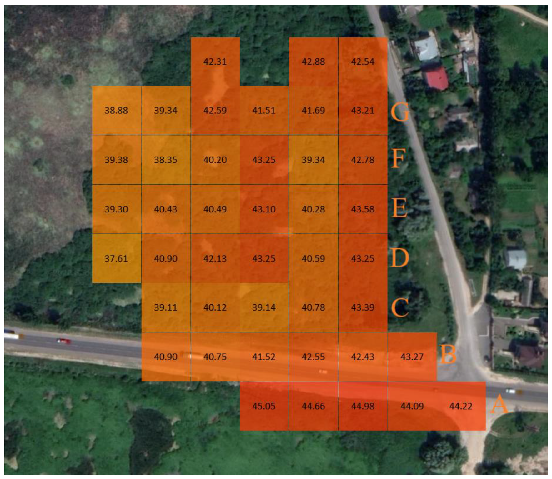
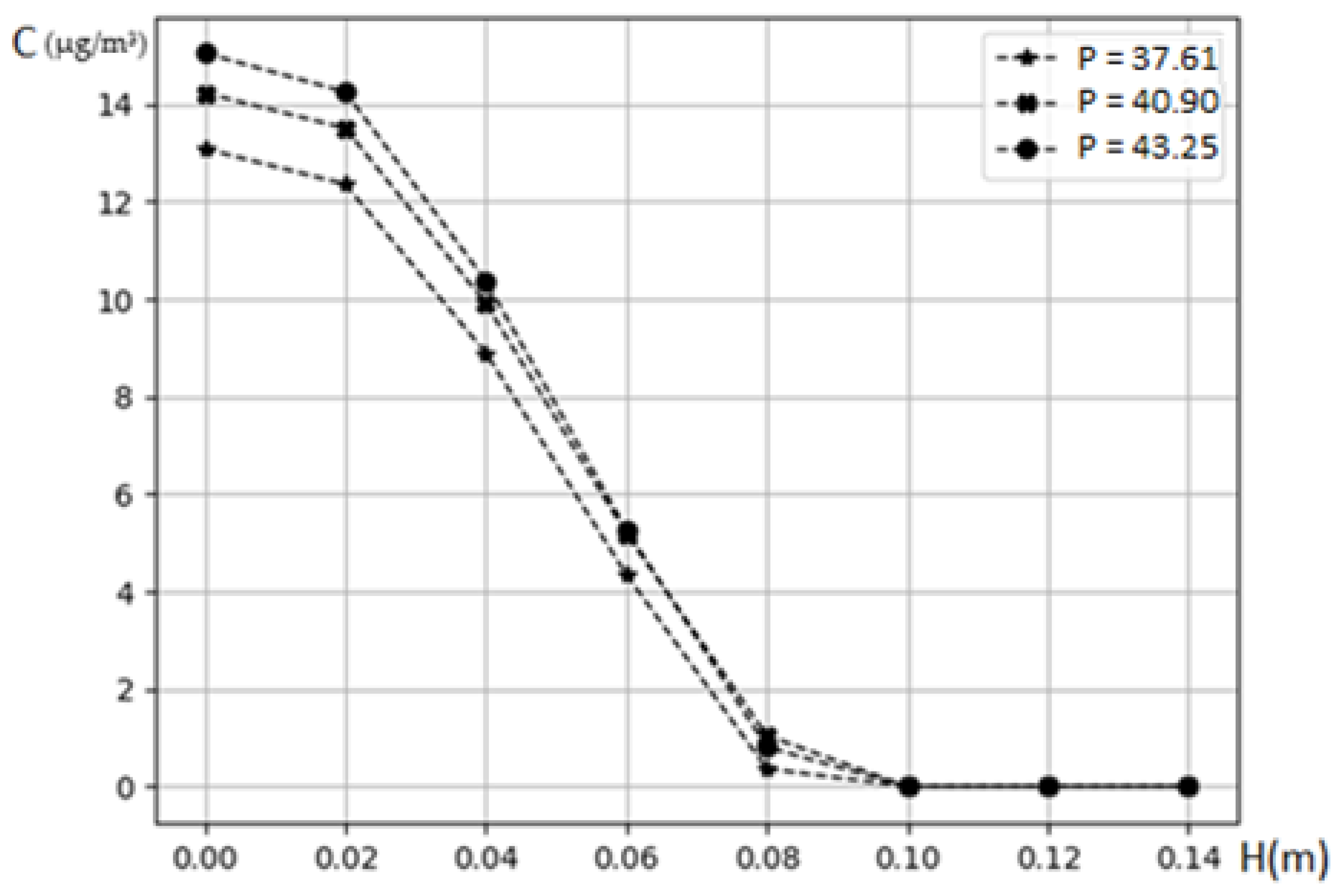
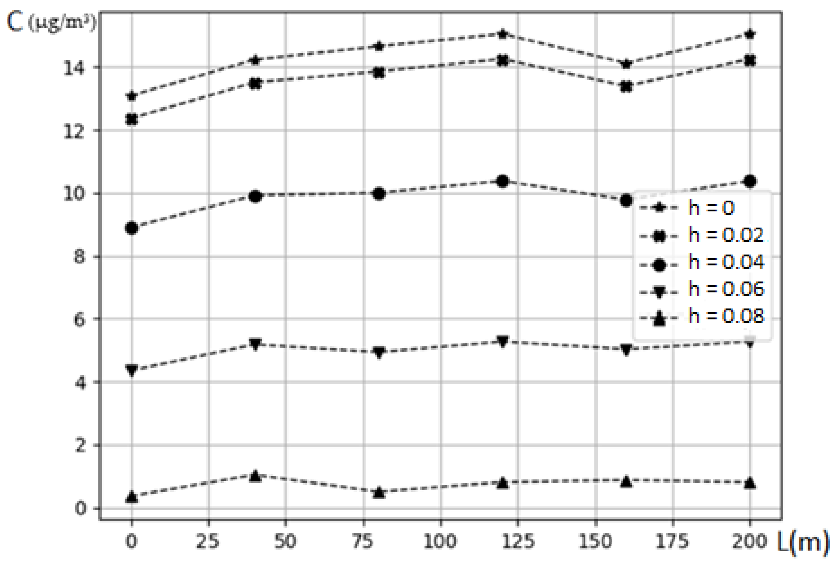
Figure 1. Monitoring system architecture.
Sustainability 13 02768 g001
Figure 2. Visualization results of dioxide nitrogen measurements at a height of 1–5 m.
Sustainability 13 02768 g002
Figure 3. Visualization results of dioxide nitrogen measurements at a height of 30 m.
Sustainability 13 02768 g003
Figure 4. Illustration of the table fragment of nitrogen dioxide measurement results generated by Sniffer4D Mapper.
Sustainability 13 02768 g004
Figure 5. Modeled concentrations of nitrogen dioxide in the soil in the neighborhood of some points of line D.
Sustainability 13 02768 g005
Figure 6. Field of nitrogen dioxide concentrations at the different distances (depths) from the soil surface in meters, for observation points of line D.
Sustainability 13 02768 g006
Figure 7. Field of concentrations of nitrogen dioxide or nitric acid at different depths of soil and waterbody (at the first point) for observation points of line G.
Sustainability 13 02768 g007
Table 1. Nitrogen dioxide measurement results (date: 2020-11-19).
LineTime
Stamp
Distance, mAir Temperature, ℃Air Humidity, %Air Pressure, Pa Concentration   of   NO 2 ,   10 6 g m 3
D (Figure 2)13:27:0504.118098,61137.61
13:27:15403.528398,59640.9
13:27:25803.528398,66042.13
13:27:351203.528398,60643.25
13:27:451603.528398,63040.59
13:27:552003.528398,60643.25
G (Figure 2)13:30:2504.118098,56738.88
13:30:35404.118098,57739.34
13:30:45803.728298,48442.59
13:30:551203.728298,46941.51
Publisher’s Note: MDPI stays neutral with regard to jurisdictional claims in published maps and institutional affiliations.

