Article

Maximizing Total Profit of Thermal Generation Units in Competitive Electric Market by Using a Proposed Particle Swarm Optimization

1
Faculty of Electrical and Electronics Engineering, Ho Chi Minh City University of Technology and Education, Ho Chi Minh City 700000, Vietnam
2
Faculty of Electrical Engineering Technology, Industrial University of Ho Chi Minh City, Ho Chi Minh City 700000, Vietnam
3
Faculty of Automobile Technology, Van Lang University, Ho Chi Minh City 700000, Vietnam
4
Power System Optimization Research Group, Faculty of Electrical and Electronics Engineering, Ton Duc Thang University, Ho Chi Minh City 700000, Vietnam
*
Author to whom correspondence should be addressed.
Sustainability 2020, 12(3), 1265; https://0-doi-org.brum.beds.ac.uk/10.3390/su12031265
Submission received: 8 January 2020 / Revised: 2 February 2020 / Accepted: 5 February 2020 / Published: 10 February 2020
(This article belongs to the Special Issue Sustainable Building Retrofit and Energy Optimization)

Abstract

:
In the paper, a proposed particle swarm optimization (PPSO) is implemented for dealing with an economic load dispatch (ELD) problem considering the competitive electric market. The main task of the problem is to determine optimal power generation and optimal reserve generation of available thermal generation units so that total profit of all the units is maximized. In addition, constraints, such as generation limit and reserve limit of each unit, power demand and reserve demand, must be exactly satisfied. PPSO is an improved version of conventional particle swarm optimization (PSO) by combining pseudo gradient method, constriction factor and a newly proposed position update method. On the other hand, in order to support PPSO to reach good results for the considered problem, a new constraint handling method (NCHM) is also proposed for determining maximum reserve generation and correcting reserve generation. Three test systems with 3, 10 and 20 units are employed to evaluate the real performance of PPSO. In addition to the comparisons with previous methods, salp swarm optimization (SSA), modified differential evolution (MDE) and eight other PSO methods are also implemented for comparisons. Through the result comparisons, two main contributions of the study are as follows: (1) NCHM is very effective for PSO methods to reach a high success rate and higher solution quality, (2) PPSO is more effective than other methods. Consequently, NCHM and PPSO are the useful combination for the considered problem.

1. Introduction

Economic load dispatch (ELD) is one of the most important problems in power systems due to its significant contributions to economy and operation stabilization of power system. The ELD problem is mathematically formulated by the objective of minimizing fuel cost and a set of constraints regarding thermal generation units and power systems [1]. The earliest ELD problem did not consider power losses in transmission lines due to effects of resistance and reactance of transmission lines and also ignored valve effects on power increase and decrease process of thermal generation units [2]. Another more complicated ELD problem has taken into account active power loss, the valve effects and complex constraints of thermal generating units such as prohibited working zones [3], ramp rate limitations [4] and generation limitations [5]. The concerned problem has been solved by applying a huge number of methods such as maximum likelihood optima (MLO) [6], evolutionary particle swarm optimization algorithm (EPSO) [7], improved stochastic fractal search algorithm (ISFSA) [8], improved social spider optimization algorithm (ISSOA) [9], interior search algorithm (ISA) [10], multi-leader comprehensive learning particle swarm optimization with adaptive mutation (MLCL-PSO) [11], dragonfly algorithm (DA) [12] and ameliorated grey wolf optimization (AGWO) [13]. In general, these studies focused on demonstrating constraint handling ability and high-quality solution searching ability of original methods and improved methods rather than proposing new issues and real phenomena regarding power systems and electric components. In fact, complicated constraints, such as generation limits, generation increase and decrease limits, prohibited working zones and active power reserve requirement, have been taken into account. On the other hand, discontinuous objective functions (i.e., fuel cost functions) have been considered to be huge challenges for solution methods. Multiple fuels and valve effects on thermal generating units were challenges. These valve effects have been represented as the sum of sinusoidal function and quadratic function meanwhile multiple fuels have been shown as a sum function of two or three quadratic functions. The challenges were the vast difficulties for optimization algorithms and ineffective algorithms could not reach global optimum solution or nearby global optimum solutions. The real effectiveness of solution methods has been confirmed by comparing fuel cost and computation speed. Clearly, the ELD problem is considered as a very important problem in power system operation; however, it can become more realistic if the competitive electric market is considered for process of electric generation and purchasing [14,15,16]. As joining competitive electricity market, thermal power plants have to supply electricity to loads with the cheapest prices and the purpose is that loads can consume the highest power energy from the thermal power plants. In this case, customers can get the highest profit by selecting the most reasonable providers among available suppliers [17]. However, thermal power plants have to cope with several difficulties. In fact, they have to decide how much active power should be generated to supply to loads and how much active power should be reserved for coming time periods [18]. If higher reserved power can be sold, higher benefit can be reached. However, if customers do not use the reserved power, thermal power plants must suffer non-benefit [19]. Optimal operation of thermal power plants in competitive electricity market has been widely and successfully studied [20,21,22,23,24,25,26,27,28,29,30,31]. Among the studies, start-up fuel cost has been concerned in some studies [20,21,22,23,24,25,26,27,28] while this cost has not been taken into account in remaining studies. Different methods have been proposed for the problem such as Lagrange function-based evolutionary programming (LFEP) [19], Tabu search algorithm (TSA) [20], muller approach (MA) [21], memetic optimization algorithm (MOA) [22], modified artificial bee colony optimization algorithm (MABCOA) [23], ant colony optimization algorithm (ACOA) [24], multi-agent model algorithm (MAMA) [25], binary fish optimization algorithm (BFOA) [26], Lagrange function-based invasive weed optimization algorithm (LFIWOA) [27], sine function and cosine function-based algorithm (SCBA) [28], binary whale optimization algorithm (BWOA) [29], expanded Lagrange function-based Hopfield network method (ELF-HNM) [30] and five Lagrange function-based Hopfield neuron network (LF-HNN) methods [31]. The main difference between studies [1,2,3,4,5,6,7,8,9,10,11,12,13] and studies [20,21,22,23,24,25,26,27,28,29,30,31] is competitive electric market. For example, the same authors have published three studies [8,9,31] in Energies journal but only the study [31] has considered competitive electricity market. Nonconvex fuel cost functions together with complicated constraints such as prohibited operating zones and ramp rate limits have been considered in the two studies [8,9]. Whereas, the complex level of the study [31] is due to competitive electricity market. In addition, applied methods in the studies are also different. Improved versions of the meta-heuristic algorithm have been applied for nonconvex economic load dispatch problem (ISFSA [8] and ISSOA [9]) whereas five LF-HNN methods have been proposed for dealing with competitive electricity market [31]. Basically, the two metaheuristic algorithms can deal with the competitive electricity market successfully but the five LF-HNN methods fail to cope with nonconvex fuel cost function. Among the studies regarding the competitive electric market, ELF-HNM was an application of Hopfield neuron network based on expanded Lagrange function. The method obtained better results than PSO and DE. However, the expanded function used one more control parameter and the determination of the parameter became a problem. Conventional Lagrange function was used to tackle the shortcoming of ELF-HNM [30]. Five different functions were proposed to update output neurons such as Logistic, Hyperbolic tangent, Gompertz, Error and Gudermanian function, leading to the appearance of five methods [31]. Among five LF-HNN methods, LF-HNN with the application of error function was the best with the most stable search ability and the highest performance. The ELF-HNM and LF-HNN have shown better search ability than metaheuristic algorithms such as PSO, DE and cuckoo search algorithm (CSA). However, the application of the traditional methods larger systems will become more difficult because the number of constraints of the problem is not small. Basically, derivative-based methods have one additional parameter for each constraint of problem and the selection of the parameter is not easy because there is not a predetermined range for the parameter. Furthermore, the methods for finding the most appropriate values are mainly based on the experiment. In addition, the methods must cope with difficulties of deterministic methods since taking partial derivative must be required. As a result, the methods could not deal with non-differential functions-based problems. Consequently, as the nonconvex fuel cost function is taken into account, the utilization of Hopfield neuron network-based methods is impossible. Therefore, meta-heuristic methods can solve the problem more easily and successfully, especially for systems with large scale and valve effects.
Based on the competitive electric market in USA [32], the study [18] has established total revenue function, total fuel cost function and total profit function for two different cases including payment for power delivered and payment for reserve allocated. As a result, reserve market problem has been mathematically formulated in the study [18] and then the formulation has been applied for unit commitment problem [19]. The unit commitment problem is also the economic load dispatch problem with considering operation status of available thermal generating units and start-up cost of the units. The combination of unit commitment with competitive electric market has been dealt in the study [19]. In our work, we have reduced the complex level of the study [19] by supposing that all available thermal generating units are working. Thus, operation status and start-up cost of the units are neglected in the paper. As a result, the problem formulation is established in Section 2 by using previous studies [18,19] about competitive electric market and other previous studies [1,2,3,4,5,6,7,8,9] about economic load dispatch problem.
Among existing metaheuristic algorithms, particle swarm optimization is a popular and effective method with simple characteristic and simple implementation [33]. However, PSO is not a new method and its performance is not really effective for all optimization problems, especially for complicated problems with complicated constraints and nondifferentiable objective function. PSO is easily fallen into local optimal zones, and the possibility of jumping out the zones and moving to global optimal zones is low. However, it is not denied that PSO has been widely and successfully applied for many optimization problems, and its improved versions have increased constantly such as MLCL-PSO for ELD problem [11], hybrid particle swarm optimization (HPSO) for power loss optimization problem in transmission networks [34], hybrid multiagent-based particle swarm optimization (HMPSO) [35], PG-PSO for ELD problem [36], time-varying acceleration coefficients-based particle swarm optimization (TVAC-PSO) for combined heat and power dispatch (CHPD) problem [37], and four PSO methods such as constriction factor-based particle swarm optimization (CF-PSO), inertia weight factor-based particle swarm optimization (IW-PSO), CF-PSO with local best particle and IW-PSO with local best particle for CHPD problem [38]. As shown in the studies, these PSO methods could reach good result with higher performance than other metaheuristic methods like DE, hybrid DE (HDE), improved DE (IDE), GA, hybrid GA (HGA), TSA, gravitational search algorithm (GSA), harmony search algorithm (HSA), evolutionary programming algorithm (EPA), simulated annealing algorithm (SAA) and biogeography-based optimization algorithm (BBOA). It is clear that PSO variants are highly effective for optimization problems in the power system field and the high-performance characteristics of these methods have high contribution to the power system. Consequently, if PSO methods continue to be improved and applied for optimization problems for further investigation of performance, researchers can select the most appropriate option for their own problem in the power system or other engineering fields. In this paper, we apply PSO variants consisting of conventional PSO [33], CF-PSO [39], IW-PSO [40], PG-PSO [41], IW-PG-PSO, CF-PG-PSO, TVIW-PSO [42], TVAC-PSO [43], and PPSO. In PPSO method, we have combined pseudo gradient method, constriction factor, and a newly proposed velocity update method. Pseudo gradient method is useful in determining better direction for moving to new positions meanwhile constriction factor can support to limit search space. The two applications can form a high-performance method, which is CF-PG-PSO. Furthermore, we also propose a new position update method by using the so-far best position of each particle instead of using the previous position in PSO. In addition, we propose NCHM that can satisfy power reserve demand easily and successfully but the effectiveness is high. For presenting the real performance of NCHM, the survey of obtained results from PPSO and eight other PSO methods with and without using NCHM is accomplished by using a three-unit system with convex fuel cost function, a ten-unit system with convex fuel cost function and a twenty-unit system with nonconvex fuel cost function. For indicating the real performance of PPSO, it is compared to these eight PSO methods, SSA, MDE and other previous methods such as PSO, DE, CSA, ELF-HNM and five LF-HNN methods. In summary, the novelties of the study are as follows:
(1)
Propose the effective NCHM for handling constraints.
(2)
Propose the high performance PPSO.
(3)
Consider valve effects on thermal generation units for the considered problem.
In addition, the application of PPSO method also has some advantages as follows:
(1)
PPSO method has few control parameters, population and the number of iterations. Therefore, the setting of the two parameters is simple.
(2)
The process of evaluating solution quality is easily and simply performed by calculating fitness function.
By owning novelties and advantages above, the study can reach the following main contributions:
(1)
Reach very high success rate with 100%: Implemented methods using NCHM always reaches all successful runs but the same implemented methods without using NCHM must suffer much lower than 100% for success rate.
(2)
Converge to high quality solutions: NCHM supports implemented methods to find global optimum solutions with fast speed and reach high stability.
(3)
PPSO method always reaches better results than other PSO, SSA, MDE and previous methods.
(4)
PPSO method is faster than approximately all other methods for study cases.
However, in order to reach good results and appropriate simulation time for PPSO method, some difficulties exist as follows:
(1)
The most appropriate values for the population and the number of iterations are not easy to select. In fact, higher values can result in better results but simulation time is still increased correspondingly. If high values are set, all methods have the same best solution and the evaluation is not exactly performed. In this case, real performance of PPSO method cannot be shown.
(2)
The procedure of applying PPSO method is a long iterative algorithm. Therefore, the implementation procedure must be careful and verification procedure must be serious.
In addition to introduction, other main sections of the paper are as follows: Mathematical formulation of the problem is shown in Section 2. The construction of applied PSO methods is expressed in Section 3. The application of the PSO methods for the problem is described in detail in Section 4. Comparison and discussion of obtained results are shown in Section 5. Finally, a summary of the contribution and future work is included in Section 6.

2. Problem Formulation

2.1. Objective Function

The ELD problem in the competitive electric market is established by the presence of an objective function and a set of constraints regarding thermal generating units as well as power systems. In order to present the considered objective function, the fuel cost function for generating electricity is first mentioned as follows:
For the case without considering valve point loading effects on thermal generation units during the electricity generation process, fuel cost function is approximately expressed as the second order function below [12]:
F n = α n + β n P G n + χ n P G n 2
However, it is more appropriate since the valve effects are considered for the operation process of the units, and a more complex function is used as follows [28]:
F n = α n + β n P G n + χ n P G n 2   + | δ n × sin ( ε n × ( L B n P G n ) ) |
In the competitive electricity market, reserve power is really necessary and thermal units must generate power higher than predetermined demand if reserve is allocated and used by loads. So, fuel cost for both reserve generation and power generation must be taken into account based on Formulas (1) and (2) above. The two new fuel cost functions are as follows:
F n = α n + β n ( P G n + R G n ) + χ n ( P G n + R G n ) 2
F n = α n + β n ( P G n + R G n ) + χ n ( P G n + R G n ) 2   + | δ n × sin [ ε n × [ L B n ( P G n + R G n ) ] ] |
In the competitive electric market, each thermal power plant concerns two cases, the payment for power delivered and the payment for reserve power. For each case, total revenue and total cost are calculated as follows:
(1) Payment for power delivered
In this case, reserve power is only paid if the reserve power is used by customers. Thus, the price of reserve power (PriceRP) is higher than the price of delivered power (PriceDP). The total revenue (TR) and total cost (TC) are calculated by [19]:
T R =   P r i c e D P × n = 1 N P G n . S t n + P r i c e R P n = 1 N r × R G n . S t n
T C = ( 1 r )   n = 1 N F n . S t n + r n = 1 N F n . S t n + n = 1 N F S U n . S t n
In the two equations above, r is the probability that reserve power is called by the requirement from loads. Stn is on/off operation status of the nth thermal generation unit. The parameter has two values only, 1 for on operation status and 0 for off operation status. In addition, FSUn is start-up fuel cost of the nth thermal generation unit. The determination of the status and the start-up fuel cost are really important for finding optimal generation and optimal reserve as unit commitment problem is considered. However, in the study, we consider pure economic load dispatch problem and the assumption is that all thermal generation units are working. Therefore, the start-up fuel cost and on/off operation status can be neglected, and the result does not influence the task of determining optimal generation and optimal reserve.
(2) Payment for reserve power
In this case, thermal power plants receive the price of reserve power because the reserve power is not used. As the reserve power is used by loads, thermal power plants receive the price for delivered power that was generated. So, the price of reserve power is much less than that of delivered power. TR and TC are obtained by [19]:
T R =   P r i c e D P × n = 1 N P G n . S t n + [ ( 1 r ) . P r i c e R P + r . P r i c e D P ] n = 1 N R G n . S t n
T C = ( 1 r )   n = 1 N F n . S t n + r n = 1 N F n . S t n + n = 1 N P r i c e D P . S t n
In Equations (7) and (8), PriceDP and PriceRP are not fixed values and they are different for different time periods in a day [18,19,44]. In fact, this issue was demonstrated [18] and different values for these prices were then applied [19]. In this paper, we consider only one period for pure economic load dispatch problem. Therefore, we only considered one fixed value for PriceDP and one fixed value for PriceRP for each study case.
Finally, the total profit (TP) is determined by [18]:
T P = T R T C
The objective function is to maximize the total profit or minimize the minus total profit as follows:
Maximize   { T P = T R T C }   o r   Minimize   { T P = T C T R   }
In the Equations (5) and (7), total reserve power from all units ( n = 1 N R G n ) can be from zero to reserve demand (RD) depending on the obtained total profit. As seen from Equation (10), total profit can be higher than zero if the total revenue is higher than total fuel cost. It can be seen from the total fuel cost functions (6) and (8), fuel cost of generation and reserve can be considered if reserve is called and used. So, Equations (5) and (7) can be obtained for any values of reserve and the profit is dependent on the revenue for selling power and total fuel cost for generating power.

2.2. The Consisdered Constraints

(1) Power demand
Basically, the ELD problem is about determining power generation of all thermal units for minimizing total cost of these units. Power balance constraint in the problem is about active power in which total generation, power loss and power demand must follow the equality constraint [45,46]. Frequency stability is really important in high voltage networks [47] because power system cannot be stably working if the frequency oscillation happens. Thus, in traditional economic load dispatch problem, active power balance is seriously constrained as the following model [45]:
T P G P l o s s D = 0
where Ploss is the total power losses in all transmission lines; TPG is total power generation of all power sources [46] that can supply electricity to loads. TPG can be expressed in detail as follows:
T P G = i = 1 I P H i + j = 1 J P P j + k = 1 K P W k + n = 1 N P G n
where PHi is the power generation of the ith hydropower plant; PPj is the jth power generation of photovoltaic system; PWk is the power generation of the kth wind turbine; and PGn is the power generation of the nth thermal generation unit; I is the number of hydropower plants; J is the number of photovoltaic systems; and K is the number of wind turbines
However, as considering competitive electricity market for economic load dispatch problem, the power balance constraint above is rewritten as follows [18,19]:
n = 1 N P G n D
On the contrary to the traditional economic load dispatch problem (neglecting competitive electric market), total power generation from N units in the problem can be lower than the forecasted power demand as long as the total profit of N units is high. Generation companies can select to purchase power lower than demand [19].
However, power generation of each thermal generating unit must follow the limits below [30]
L B n P G n U B n
(2) Reserve power demand
In the current industry, the significance of the total mean electricity cost can be directly found in the requirement to satisfy the (N-1) contingency [48]. However, two high changes in the competitive industry that are taking place can lead to the high deviations from the operation concept [18]. In the studies [32,49], the reasons for making reserve markets and reserve generation contract were presented. First, power energy providers will sell power energy to their customers via signed contracts. In order to avoid the service interruption and compensate customers for the interruption due to the failure of their own generator, the power energy providers may buy reserve power energy from other providers. Second, since industrial zones or other high-power energy customers usually move to deregulation of use of electricity, reserve market is really necessary. Namely, the reserve demand constraint is formulated by:
n = 1 N R G n R D
Similar to power generation, total reserve power of all units can be lower than reserve demand as long as total profit is high and generation companies can purchase reserve lower than the forecasted reserve demand [19].
However, reserve capability of each thermal generating unit is not infinite and constrained by [18,19]:
0 R G n U B n L B n
R G n + P G n U B n
As showing constraints (16) and (17) above, reserve generation limits of each thermal generating unit are not fixed for different reserve demand and power demand. The limits are dependent on power generation, which was predetermined. This issue is totally different from power generation limits that are shown in constraint (14). So, the study focuses on a good method to reach the most appropriate limits for reserve generation and find the best reserve power for each unit in competitive electricity market. In general, previous studies have ignored the major issue.

3. Applied PSO Methods

3.1. CF-PSO and IW-PSO

In 1995, Kennedy and Eberhart [33] developed conventional PSO to solve the optimization problem and then the method was modified to be more effective for more complicated problems [39,40,41,42,43]. PSO method is represented as two typical terms including velocity and position. The two main factors are formulated by:
V e p n e w = V e p + c 1 . ε 1 . ( P o b e s t , p P o p ) + c 2 . ε 2 . ( P o G b e s t P o p )
P o p n e w = P o p + V e p n e w
The process of updating new velocity by using (18) was considered to be limited due to the constant change of velocity [39,40]. Then, inertia weight factor [39] and constriction factor [40] were proposed for finding out more promising velocity. The application of the two factors results in the following model:
V e p n e w = ω V e p + c 1 . ε 1 . ( P o b e s t , p P o p ) + c 2 . ε 2 . ( P o G b e s t P o p )
V e p n e w = C F . [ V e p + c 1 . ε 1 . ( P o b e s t , p P o p ) + c 2 . ε 2 . ( P o G b e s t P o p ) ]
where:
ω = ω max . ω max ω min G max . G
C F = 2 | 2 ( c 1 + c 1 ) ( c 1 + c 1 ) 2 4 ( c 1 + c 1 ) |
In CF-PSO and IW-PSO, position update still utilizes Formula (19).

3.2. TVIW-PSO and TVAC-PSO

The combination of inertia weight factor and constriction factor has been applied to develop TVIW-PSO method [42]. The proposal developed the new velocity as follows:
V e p n e w = C F . [ ω V e p + c 1 . ε 1 . ( P o b e s t , p P o p ) + c 2 . ε 2 . ( P o G b e s t P o p ) ]
On the contrary, the study [43] has proposed the change for two acceleration coefficients c1 and c2, and the new velocity of TVAC-PSO is determined by:
V e p n e w = V e p + c 1 . ε 1 . ( P o b e s t , p P o p ) + c 2 . ε 2 . ( P o G b e s t P o p )
where
c 1 = ( c 1 E n d c 1 i n i t i a l ) G G max + c 1 i n i t i a l
c 2 = ( c 2 E n d c 2 i n i t i a l ) G G max + c 2 i n i t i a l
In the two equations above, c1initial and c1End are initial and final cognitive acceleration factors, respectively. c2initial and c2End are initial and final social acceleration factors, respectively. The factors are predetermined and fixed during the application of TVAC-PSO for a typical optimization problem.

3.3. PG-PSO

The pseudo-gradient based search algorithm (PGBSA) [41] has been proposed with intent to select a more appropriate velocity direction for each considered particle. PGBSA could enable PSO to determine the best direction in a large search space without requesting any complicated computation process. The application of PGBSA for PSO has developed PG-PSO and it has been implemented for nonconvex economic load dispatch problem with complicated constraints and non-differentiable objective function [41]. The method for updating new velocity in PG-PSO still applied formula of PSO meanwhile the method for updating new position is determined by:
P o p n e w = { P o p + α ( P o p n e w ) . | V e p n e w |   i f   F p < F p Pr e P o p + V e p n e w    e l s e
where α ( P o p n e w ) is direction determination factor and calculated by using the equation below.
α ( P o p n e w ) = { 1 i f   P o p < P o p P r e 0 i f   P o p = P o p P r e 1 e l s e

3.4. The Proposed PSO Method

In this paper, we suggest applying the combination of PG-PSO with inertia weight factor to form IW-PG-PSO and the combination of PG-PSO with constriction factor to form FC-PG-PSO. In addition, we suggest one more modification for updating new positions as follows:
P o p n e w = { P o b e s t , p + α . | V e p n e w |   i f   F p < F p Pr e P o b e s t , p + V e p n e w    e l s e
By applying the combination of FC-PG-PSO and the newly updated position model, PPSO is first introduced in the paper. In summary, PPSO method applies Formulas (21) and (23) to update new velocity and then applies Formulas (29) and (30) to update new position.

4. Implementation of PPSO Method for the Considered Problem

4.1. The New Constriaint Handling Method for Reseve Power

As shown in Equation (14), reserve power of each thermal generating unit n can be from 0 MW to (UBn-LBn) but it is totally different if Equation (17) is considered as another main constraint. In fact, Equation (17) indicates that the reserve must not be higher than (UBn-PGn) while PGn can be higher than LBn. So, we suggest that upper bound of reserve should be determined first and then real reserve can be constrained by the upper bound. Namely, the two formulas below should be used.
R G n max U B n P G n
0 R G n R G n max
Therefore, in order to sure reserve power always satisfy constraints (16) and (17), the upper bound of reserve should be determined first by using Equation (31) and then its value is checked and corrected by the following model:
R G n = { 0 i f   R G n 0 R G n max i f   R G n R G n max R G n e l s e

4.2. Main Steps of the Proposed Method for the Implementation

4.2.1. Selection of Control Variables and Population Initialization

Basically, each solution p contains a set of control variables corresponding to considered problems. In the paper, power generation and reserve generation are selected to be control variables and included in each solution p (Pop) as the following expression:
P o p = [ P G n , p ,   R G n , p   ] ;   n = 2 , ,   N
The solution Pop is not infinite and seriously constrained by the upper bound PoUB and lower bound PoLB, which are, respectively, determined by:
P o U B = [ U B n ,   ( U B n L B n )   ] ;   n = 2 ,   ,   N
P o L B = [ L B n ,   R G n min   ] ;   n = 2 ,   ,   N
where R G n min is the minimum reserve generation of the nth thermal generating unit and is equal to 0, as shown in Equation (32).
After determining control variables and their limitations, solution Pop (where p = 1, …, Nop) in the population is randomly produced by:
P o p = P o L B + ε 3 . ( P o U B P o L B ) ;   p = 1 ,   ,   N o p

4.2.2. Calculation of Dependent Variables

After having power generation and reserve generation from unit 2 to unit N, the power generation and the reserve generation of the first thermal generating unit is determined by
P G 1 D n = 2 N P G n
R G 1 R D n = 2 N R G n

4.2.3. Correction for Produced Control Variables

After initializing solutions by using Equation (37), reserve generation must be checked and corrected if it is outside the range between lower bound and upper bound. The correction for reserve can be accomplished by using Section 4.1.
In addition, after updating new solutions by using Equation (30), power generation must be also corrected by using Equation (40) below:
P G n = { L B n i f   P G n L B n U B n i f   P G n U B n P G n e l s e ;   n = 2 ,   ,   N
Finally, reserve generation continues to be corrected by using Section 4.1.

4.2.4. Handling Violation of Power Demand and Reserve Demand

After determining power generation and reserve generation by using Section 4.2.2, power demand and reserve demand are checked and penalized if violations happen. Two penalty terms corresponding to the violation of power demand and reserve demand are calculated by using the following models:
Δ D p = { 0 i f   n = 1 N P G n , p D ( n = 1 N P G n , p D ) 2 e l s e
Δ R D p = { 0 i f   n = 1 N R G n , p R D ( n = 1 N R G n , p R D ) 2 e l s e

4.2.5. Handling Violation of the First Thermal Generating Unit

Power generation and reserve generation of the first thermal generating unit cannot be corrected because they have a huge contribution to exactly met power demand and reserve demand. Thus, penalty terms for the violations of the first thermal generating unit must be taken into account and determined by:
Δ P G 1 , p = { ( P G 1 , p P G 1 min ) 2 i f   P G 1 , p < P G 1 min ( P G 1 , p P G 1 max ) 2 i f   P G 1 , p > P G 1 max 0 e l s e
Δ R G 1 , p = { ( R G 1 , p R G 1 min ) 2 i f   R G 1 , p < R G 1 min ( R G 1 , p R G 1 max ) 2 i f   R G 1 , p > R G 1 max 0 e l s e

4.2.6. Fitness Function

Fitness function must be calculated to evaluate the quality of solutions. Hence, the fitness function has to point out the quality of objective function and the violation level of constraints and dependent variables. In an ELD problem with the competitive electric market, the fitness function is the sum of minus total profit and penalty terms for the violations of power demand, reserve demand and the first thermal generation unit. In case of finding a valid solution, fitness function and the minus total profit are the same meanwhile penalty terms are zero. Nevertheless, there is no warrantee that the valid solution is the global optimum or close to the global optimum. In the study, the fitness function is expressed as follows:
F p n e w = ( T C T R ) + K 1 . Δ D p + K 2 . Δ R D p + K 3 . Δ P G 1 , p + K 4 . Δ R G 1 , p
where K1, K2, K3 and K4 are penalty factors and determined by experiment.

4.3. Establishing Limits of Velocity and Producing Initial Velocity

The upper limit and lower limit of velocity are respectively determined by:
V e U B = L i m . ( P o U B P o L B )
V e L B = L i m . ( P o U B P o L B )
where Lim is the velocity limit factor and can be selected from 15% to 20% [36].
Similar to initial solutions, initial velocity has to be determined by:
V e p = V e L B + ε 4 . ( V e U B V e L B ) ;   p = 1 ,   ,   N o p

4.4. Termination Criterion for Iterative Algorithm

Generally, termination criteria for an iterative algorithm in solving optimization problems can be maximum mismatch of considered constraints, error tolerance of two consecutive iterations or the number of iterations dependent on characteristic of implemented methods and characteristic of considered problems. In the study, PPSO is a population-based method and heavily influenced by random factors. Consequently, the number of iterations is used for the stopping criterion and collecting results. A high possibility is that the high number of iterations can result in better optimal solutions and more stable search ability. Thus, the search process is carried out until the last iteration is reached. The most appropriate selection of the iteration is reached by experiment. However, the performance of a run is heavily influenced by iterations and population. PPSO handles constraints (13) and (15) by selecting reasonable control variables shown in (34) and other constraints (14), (16)–(17) by correcting and using other penalty methods in Equations (31)–(44) so that considered constraints are exactly met. One solution is considered as a valid one if there is no violation of the considered constraints. Normally, one solution found by using the optimization algorithm, which is called the optimal solution, does not necessarily have good quality. For an implemented run, if the total profit is equal to fitness function at the last iteration (i.e., G = Gmax), it is a successful run. On the contrary, if fitness function is higher than total profit (corresponding to penalty terms in (41)–(44) are higher than zero), there is at least one violated constraint and this is an unsuccessful run.

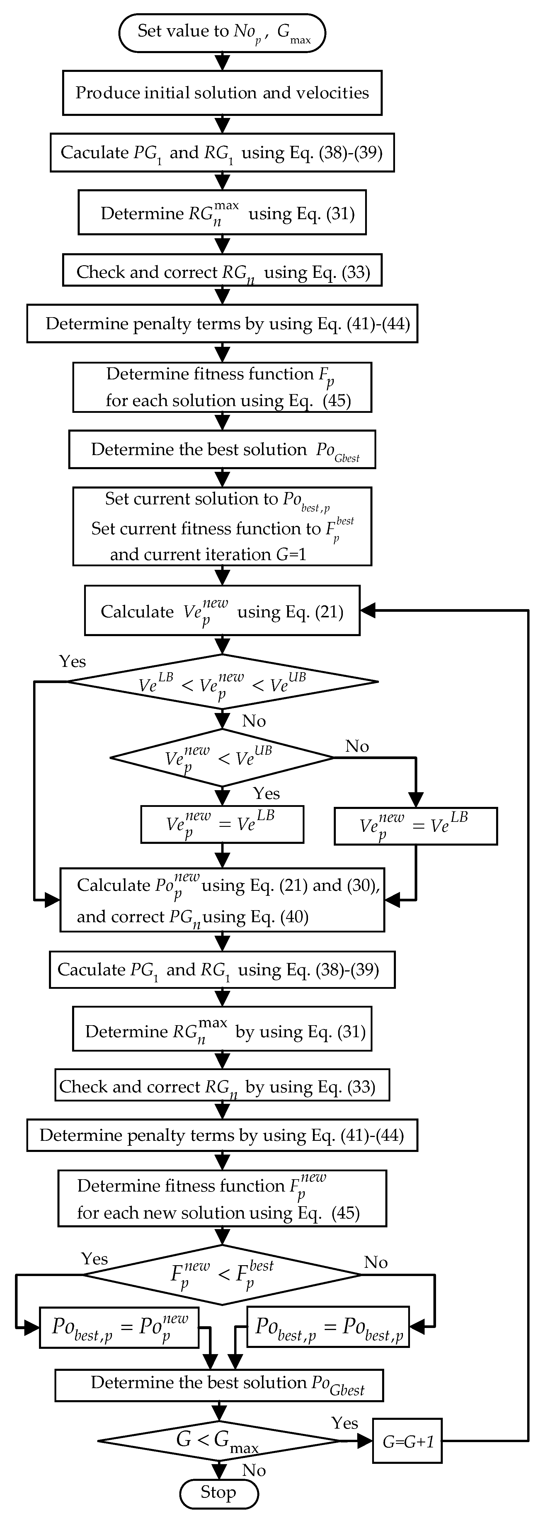
4.5. The Entire Search Process of PPSO for the Considered Problem

The whole search process of PPSO can be summarized in Figure 1 and described in the following computation steps.
Step 1: Set value to Nop and Gmax for the proposed method.
Step 2: Produce initial solutions and initial velocities by using (37) and (48), respectively.
Step 3: Calculate PG1 and RG1 by using (38) and (39), respectively.
Step 4: Determine R G n max (n = 1, …, N) by using Equation (31).
Step 5: Check and correct RGn (n = 1, …, N) by using (33).
Step 6: Determine penalty terms for the violation of power demand, reserve demand, power generation of the first thermal generating unit and reserve generation of the first generating unit by using Equations (41)–(44).
Step 7: Determine fitness function for each solution by using (45).
Step 8: Among current solutions, determine the best solution with the lowest fitness function and set to PoGbest.
Step 9: Set current solutions to PoGbest and current iteration G to 1.
Step 10: Calculate V e p n e w by using (21) and correct V e p n e w if it is oust side limits. Namely, V e p n e w is set to VeLB if V e p n e w < VeLB and V e p n e w is set to VeUB if V e p n e w > VeUB.
Step 11: Calculate P o p n e w by using (21) and (30) and correct PGn (n = 2, …, N) by using (40).
Step 12: Calculate PG1 and RG1 by using (38) and (39), respectively.
Step 13: Determine R G n max (n = 1, …, N) by using Equation (31).
Step 14: Check and correct RGn (n = 1, …, N) by using (33).
Step 15: Determine penalty terms for the violation of power demand, reserve demand, power generation of the first thermal generating unit and reserve generation of the first generating unit by using (41)–(44).
Step 16: Determine fitness function for each solution by using (45).
Step 17: Compare Pobest,p and P o p n e w (p = 1, …, Nop) to keep better one, and set kept one to Pobest,p.
Step 18: Among current solutions Pobest,p, determine the best solution with the lowest and set to PoGbest.
Step 19: If G = Gmax, stop search process. Otherwise, set G = G + 1 and back to Step 10.

5. Numerical Results

In this section, we have implemented nine methods including PSO, CF-PSO, IW-PSO, PG-PSO, IW-PG-PSO, CF-PG-PSO, TVIW-PSO, TVAC-PSO and PPSO for three test systems with two different cases. The summary of the test systems and the two considered cases is as follows:
  • Test system 1: Three units with convex fuel cost function shown in Equation (1)
  • Test system 2: Ten units with convex fuel cost function shown in Equation (1)
  • Test system 3: Twenty units with nonconvex fuel cost shown in Equation (2)
  • Case 1: Total revenue and total fuel cost are obtained by using Equations (5) and (6)
  • Case 2: Total revenue and total fuel cost are obtained by using Equations (7) and (8)
The whole data of the tests and parameters corresponding to the two cases are given in Table A1, Table A2, Table A3, Table A4 in the Appendix A. All implemented methods are coded on Matlab program language-version R2016a and run on a personal computer with configuration as follows: CPU: Intel Core i7 with 2.4 GHz processor and 4 GB of RAM 4 GB, GPU: Intel HD Graphics 5500, and system version: Windows 8.1 Pro-64-bit. For each study case, 50 successful runs are obtained. Basic parameters of PSO methods are selected as follows:
(1)
Nop = 5 and Gmax = 5 for test system 1
(2)
Nop = 20 and Gmax = 100 for test system 2
(3)
Nop = 30 and Gmax = 500 for test systems 3

5.1. The Impact of the Proposed NCHM on Results

In this section, we have run nine methods with and without using NCHM. Obtained results that are used for comparison are success rate (SR) of reaching 50 successful runs, the maximum total profit (MTP) and the average total profit (ATP). MTP is the best profit over 50 successful runs meanwhile ATP is the average profit of 50 successful runs. MTP is used to evaluate the ability of finding the best optimal solution meanwhile ATP is used to reflect the stability of the method over 50 successful runs. SR is compared to reflect the ability of dealing with all constraints of applied methods. Normally, methods with higher MTP are more effective because it can find better solutions; however, real improvement of the methods can be further investigated as considering ATP for comparison. In fact, ATP is the average value of 50 successful runs and higher ATP is corresponding to higher quality of 50 successful runs. ATP is more valuable for a small-scale system like the three-unit system since MTP of methods with and without CHM is not highly different, it is even considered approximately the same. However, ATP of methods with and without CHM is much different. In this case, methods with higher ATP is more effective and more stable for finding optimal solutions over a number of successful runs. So, ATP is really necessary for comparison and evaluation. Furthermore, for a more exact comparison, we also calculate higher MTP and higher ATP that methods using NCHM can reach as compared to the same methods without using NCHM. Then, the values are converted to percent, which is similar to the improvement level of NCHM.
As a result, all methods with using NCHM can reach 100% for success rate, but the success rate from these methods without using NCHM is only from 83.3% to 92.5%. Figure 2 and Figure 3 show MTP and ATP for case 1 and case 2 of system 1. Similarly, Figure 4 and Figure 5 show MTP and ATP for the two cases of system 2, and Figure 6 and Figure 7 show MTP and ATP of the two cases of system 3. In these figures, the bars in blue and red are MTP values with and without using NCHM, while the bars in grey and yellow are ATP values with and without using NCHM. It is seen that MTP with and without using NCHM is approximately equal for system 1, while MTP with using NCHM is higher than MTP without using NCHM for system 2 and system 3. On the contrary, ATP with using NCHM is always much higher than ATP without using NCHM for two cases of three systems. The comment is the same for MTP and ATP of nine implemented methods.
Table 1, Table 2 and Table 3 report better MTP and ATP (in $/h and in %) of methods using NCHM as compared to the same methods without NCHM. Table 1 sees that using NCHM can reach higher MTP from $0.015 to $1.450 for case 1, and from $69.056 to $179.722 for case 2 of system 1. The higher value is similar to the improvement level from 0.001% to 0.132% for case 1 and from 0.037% to 0.133% for case 2. It is clear the MTP is not much improved by using NCHM, but the improvement of ATP is much more significant. In fact, better value of ATP is from $69.056 to $179.722 for case 1 and from $142.252 to $314.008 for case 2. The values are equivalent to the high improvement from 7.347% to 22.305% for case 1 and from 15.825% to 42.9% for case 2. Table 2 shows that MTP can be higher from $39.15 to $938.57 corresponding to the improvement level from 0.27% to 6.89%, and ATP can be higher by from $1741.05 to $4117.138 corresponding to the improvement level from 13.98% to 41.75% for case 1 of system 2. For case 2, MTP can be higher by from $109.84 to $531.67 corresponding to the improvement level from 0.81% to 4.06%, and ATP can be higher by from $9357.84 to $13,026.5 corresponding to the improvement level from 1544.92% to 11,313.34%. Table 3 shows that MTP can be higher up to $425.54 corresponding to the improvement level of 2.09% and ATP can be higher up to $2263.72 corresponding to the improvement level of 12.55% for case 1. For case 2, MTP can be higher up to $286.23 corresponding to the improvement level of 1.97% and ATP can be higher up to $2376.208 corresponding to the improvement level of 20.24%.
In summary, the application of NCHM can support methods to reach significant achievements as follows:
(1)
Methods using NCHM can reach the highest SR with 100% but SR of the methods without using NCHM is much lower, only from 83.3% to 92.5%.
(2)
NCHM can support methods to find the global optimum solutions, high search stability and low possibility to low quality solutions.

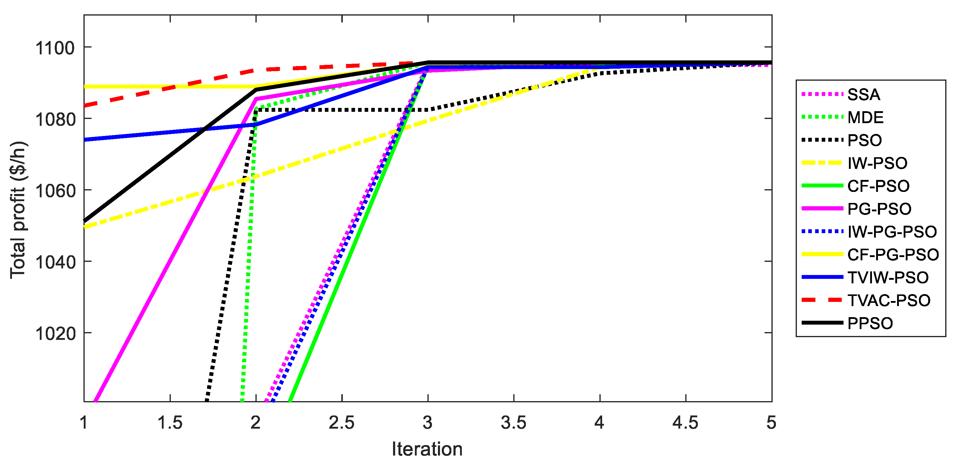
5.2. Comparison for Test System 1

In this section, we compare the real performance of the proposed PSO method with other PSO and previous methods as testing on three-unit system. In addition, we have also implemented salp swarm algorithm (SSA) [50] and modified differential evolution (MDE) [51] by setting the same population and the number of iterations as PSO methods.
Table 4 and Table 5 show the result comparison for case 1 and case 2, respectively. The comparisons indicate that PPSO can reach better MTP and ATP values than other implemented PSO methods, SSA and MDE for the two cases. MTP and ATP of PPSO are respectively $1102.451 and $1008.9942 for case 1, and $1095.648 and $1063.955 for case 2 but those of others are lower. For instance, MTP of others is from $1102.024 to $1102.4502 and ATP of others is from $935.3537 to $1006.0338 for case 1. Similarly, MTP of others is from $1094.993 to $1095.648 and ATP of others is from $872.2816 to $1056.866 for case 2. Clearly, PPSO can find the best optimal solution with the highest profit and all runs of PPSO reach higher performance than other PSO methods, SSA and MDE. Furthermore, PPSO is a more stable method in the searching process since its standard deviation (STD) is much lower than these methods. Namely, it is 96.4 for case 1 and 97.3 for case 2 whereas that of other ones is increased from 101.6 to 196.7 for case 1 and from 110.1 and 212.5 for case 1.
As compared to other remaining methods such as ELF-HNM [30], PSO [31], CSA [31], DE [31] and five Hopfield Lagrange network-based methods [31], PPSO can reach the same best solutions as approximately all these methods excluding LF-HLN-GdF [31], LF-HLN-GF [31] and LF-HLN-LF [31] for case 2 with worse solutions than PPSO. In connection with the comparison of ATP, PPSO is more effective than other metaheuristic algorithms like PSO and DE but the achievement is not reached again as comparing to CSA and five Hopfield Lagrange network-based methods. However, PPSO is still superior to these methods since it has been run by setting 5 to population and 5 to iterations and spent less computation time. In fact, DE, PSO and CSA have been implemented by using 5 for population and 500 for the number of iterations meanwhile these five Hopfield Lagrange network-based methods are deterministic algorithms with very small change among different runs.
Figure 8 and Figure 9 show the best convergence characteristics corresponding to the best run over 50 successful runs while Figure 10 and Figure 11 illustrate the mean solution searching characteristic of the 50 successful runs for case 1 and case 2, respectively. The four figures have the same manner that PPSO is slower than other ones at the first iterations but PPSO converges to better solutions at final iterations. Figure 8 and Figure 9 are about the maximum total profit, so all methods have the same final point. On the contrary, Figure 10 and Figure 11 are about the average total profit, so the final point of PPSO is much higher than that of other ones. It is clear that PPSO has better ability of jumping out local zones and converge to more promising zones.
In summary, PPSO can improve result more effectively than other PSO methods and it can reach approximately equal or better results than other ones, however, it is always faster than other ones. Therefore, PPSO is really a highly efficient method for the system with 3 units and convex fuel cost function.

5.3. Comparison for Test System 2

In this section, we compare the real performance of the proposed PSO method with other PSO, SSA and MDE and previous methods by using the ten-unit system without valve effects of thermal units. Table 6 and Table 7 show result comparison for case 1 and case 2 of the system. From the tables, it is seen that PPSO can reach better MTP and ATP than other implemented PSO, SSA and MDE methods for the two cases. MTP and ATP from PPSO are respectively $14,564.74 and $14,193.08 for case 1 and $13,635.12 and $13,525.28 for case 2 whereas those from other implemented methods are much worse. In fact, SSA must suffer the worst MTP with the lowest values of $14,370.95 for case 1 and $13,597.06 for case 2 whereas the second-best methods consisting of CF-PSO and TVIW-PSO can reach $14,563.77 for case 1 and the second-best method, IW-PG-PSO, can reach $13,635.04 for case 2. Similarly, ATP of the worst method and the second-best method is $13,918.55 and $14,128.56 for case 1 and is $13,086.99 and $13,454.77 for case 2. Clearly, all methods cannot reach the highest profit and find the global optimal solution that PPSO can. Furthermore, the stability of PPSO is always better since the standard deviation is also much lower than other ones. The standard deviation of PPSO is 236.9 for case 1 and 105.1 for case 2 whereas that of others is from 237.1 to 617.6 for case 1 and from 109.8 to 605.7 for case 2. The convergence characteristic for the best run and mean solution searching characteristic for 50 successful runs are respectively plotted in Figure 12, Figure 13, Figure 14 and Figure 15 for the two cases. As seen in Figure 12 and Figure 13, PPSO cannot reach better solutions than other ones at the first 20 iterations, however, PPSO can find better solutions. Moreover, the superiority of PPSO over other ones can be clearly seen through Figure 14 and Figure 15. Mean convergence curves of PPSO have much higher profit than those of other ones for both case 1 and case 2 from the first iteration to the last one. This means that PPSO has stronger search ability than other ones.
As compared to other remaining methods [30,31], PPSO can reach better MTP than approximately all methods for the two cases excluding LF-HLN-EF, LF-HLN-THF and ELF-HNM for case 1. Especially, as comparing to PSO [31], DE [31] and CSA [31], PPSO can reach much higher MTP and ATP. PPSO can reach higher MTP than PSO, CSA and DE by $382.55, $0.69 and $511.71 for case 1, and $1406.67, $929.64 and $1471.55 for case 2. Similarly, PPSO can also reach much higher ATP than PSO, DE and CSA for the two cases. Clearly, the improvement of PPSO over PSO, DE and CSA is significant. Although PPSO can reach higher ATP than all methods, PPSO has implemented only 100 iterations with population of 20, whereas, PSO, DE and CSA have used 500 iterations and population of 5. Furthermore, computation time of the proposed method is still much faster than these methods.
In summary, PPSO can find better or the same solutions with other compared methods but it outperforms these methods in terms of convergence speed and stability of searching ability. Consequently, PPSO is really effective for the system with ten units and without valve effects of thermal units.

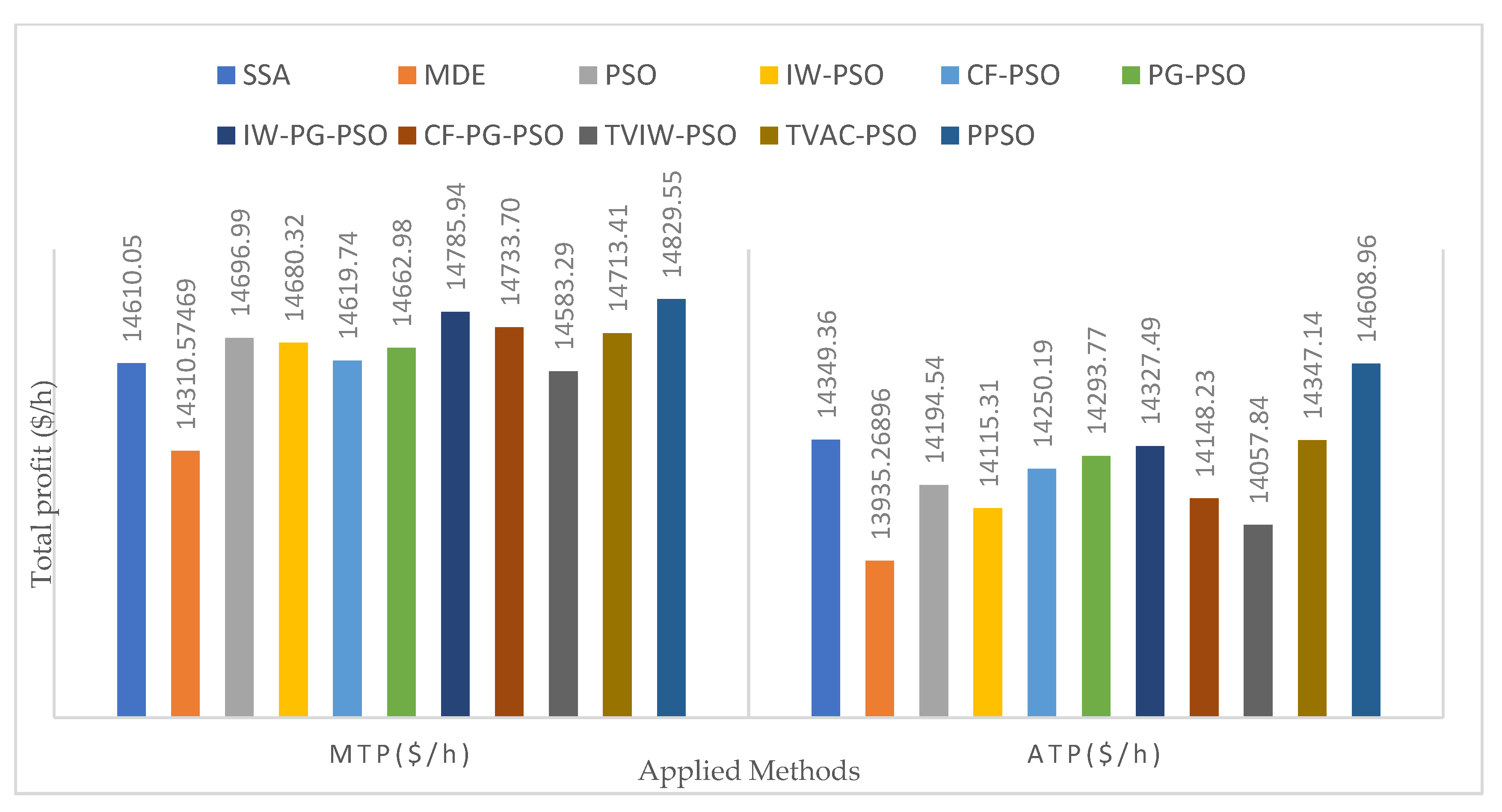
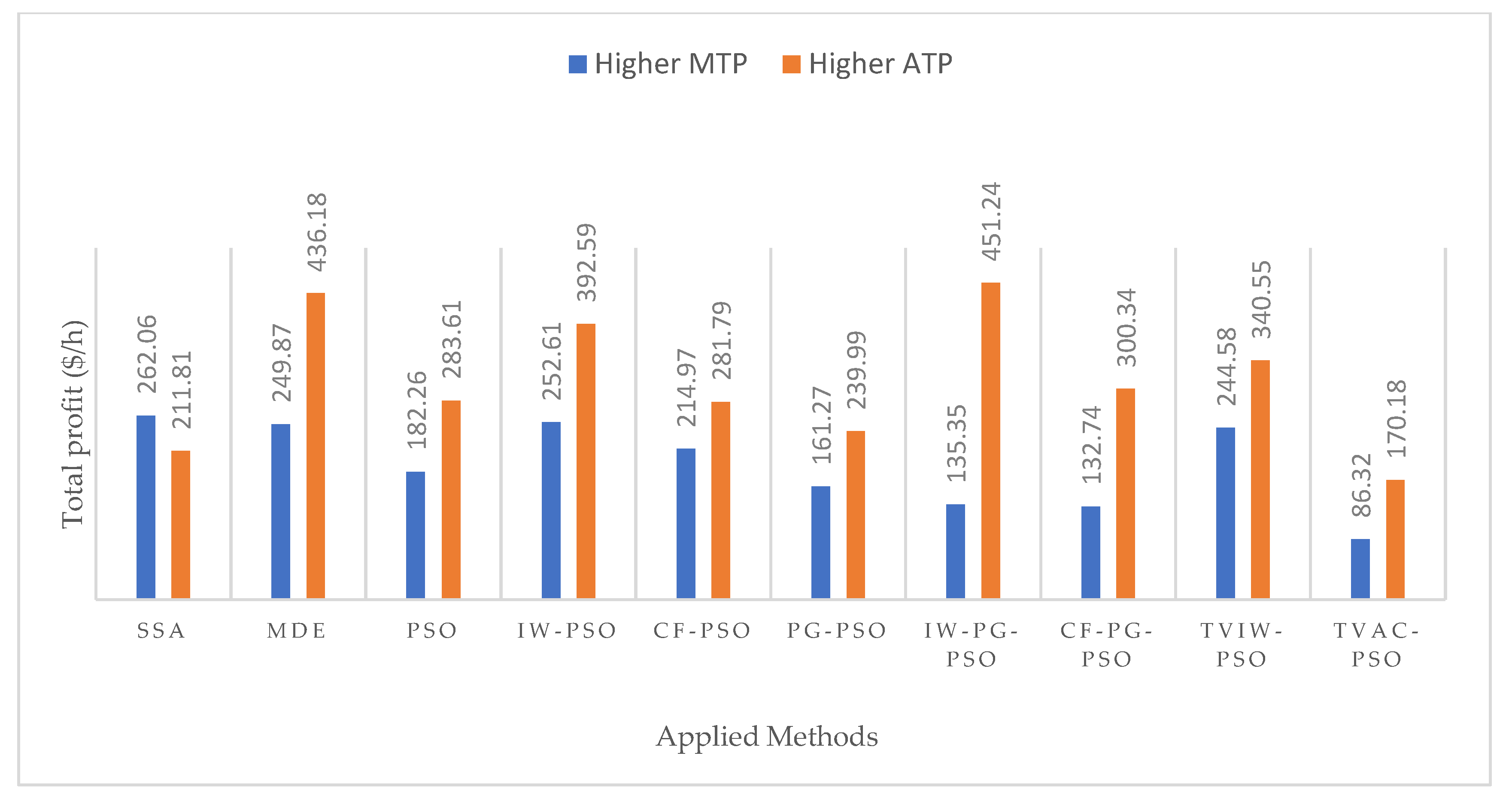
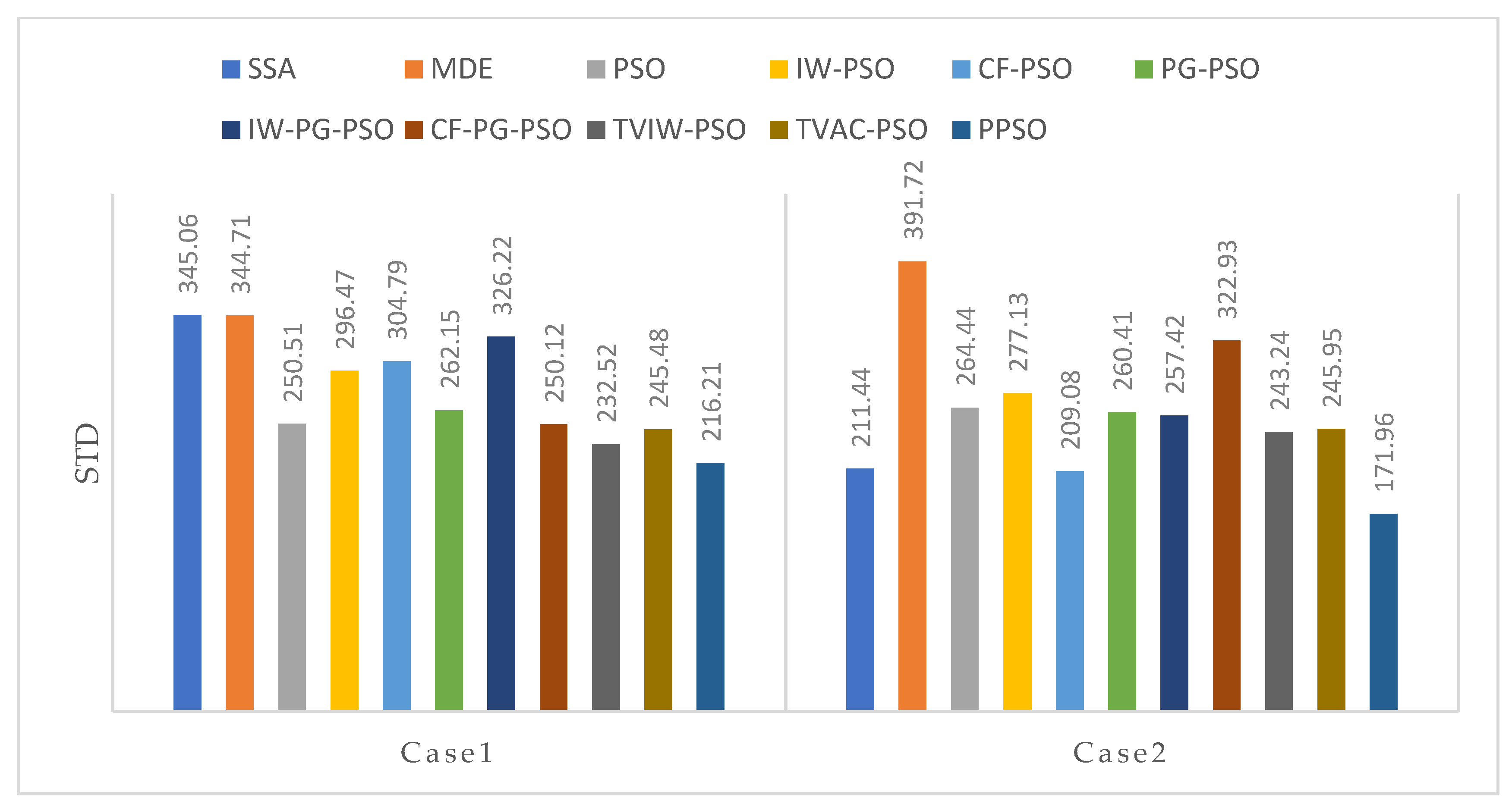
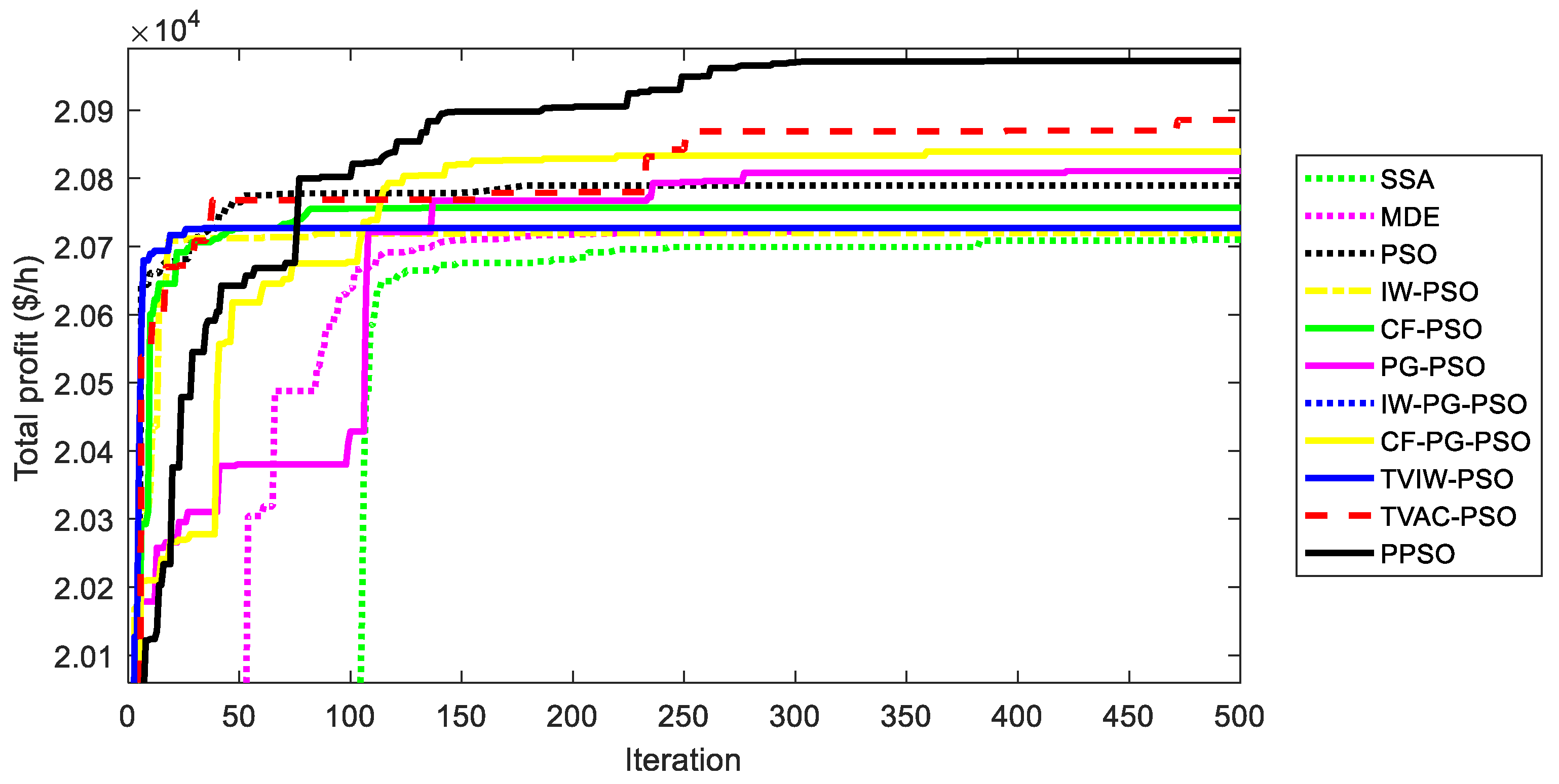
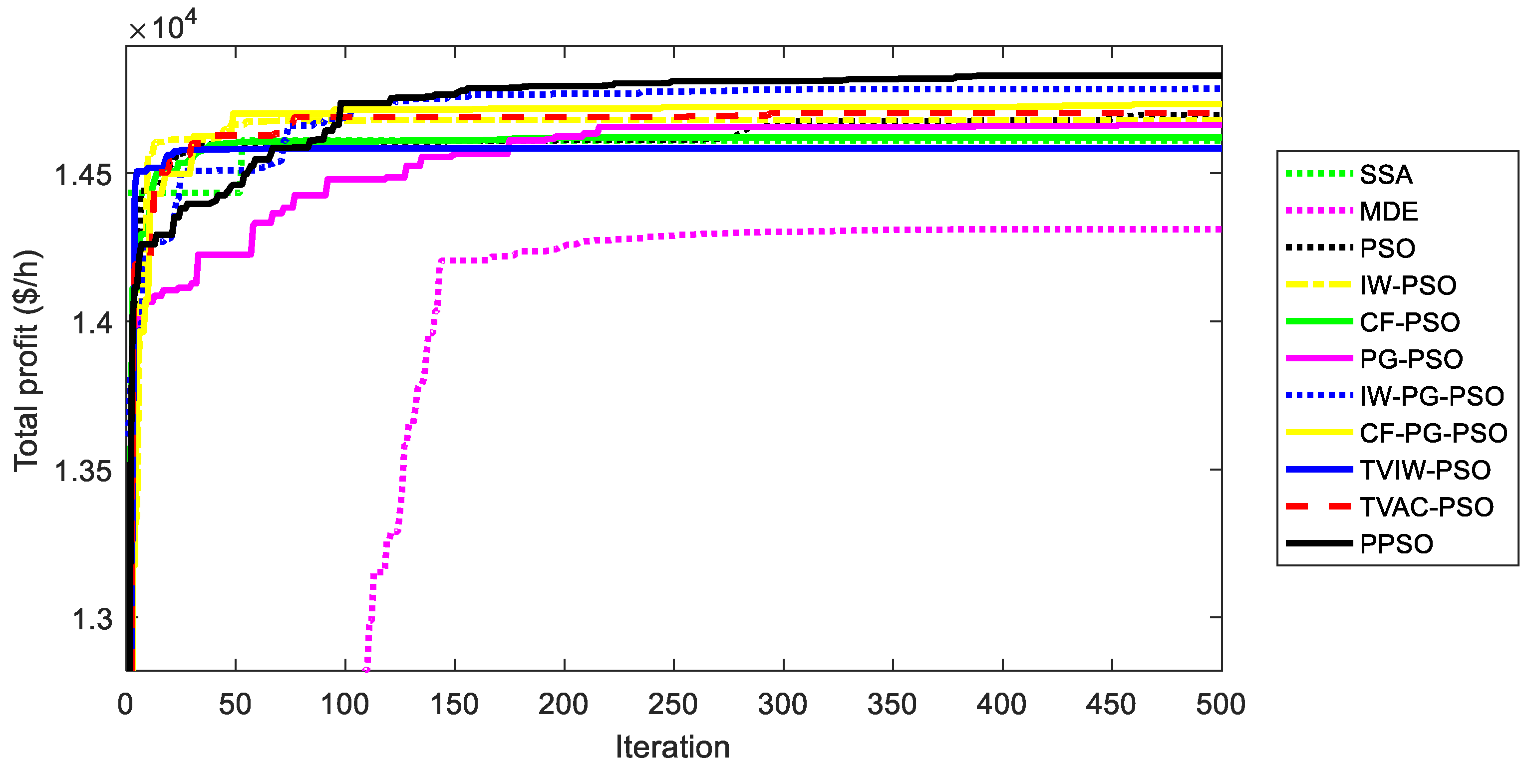
5.4. Comparison for Test System 3

In this section, PPSO is compared to eight other PSO methods, SSA and MDE by employing a 20-unit system with valve effects on thermal generation units. MTP and ATP obtained by all implemented methods are respectively plotted in Figure 16 and Figure 17. As shown in the two figures, PPSO is the best method with the highest bars of MTP and ATP for both case 1 and case 2. Higher ATP values of PPSO as comparing to other ones are significant for the two cases. For better view of the superiority, Figure 18 and Figure 19 are plotted to report higher MTP and ATP values obtained by PPSO as compared to other methods. As observing from the figures, PPSO can reach higher MTP values than other method by from $86.32 to $252.61 for case 1, and from $43.61 to $246.26 for case 2. Similarly, PPSO can reach higher ATP values than others by from $170.18 to $451.23 for case 1, and from $261.82 to $551.12 for case 2. The results are corresponding to the improvement level from 0.63% to 1.22% for MTP and from 1.2% to 2.24% for ATP of case 1. For case 2, the improvement is from 0.29% to 1.69% for MTP and from 1.82% to 3.92% for ATP. Figure 20 showing standard deviation of 50 successful runs is also a good evidence for confirming the strong search of PPSO since two bars of PPSO for the two cases are the lowest among eleven implemented ones.
As seen from the computation time shown in Figure 21, all applied methods have approximately equal time because we have set the same population and the same number of iterations for them. So, simulation time is approximately the same. However, the convergence characteristics of the best run and the mean solution searching characteristics in Figure 22, Figure 23, Figure 24 and Figure 25 for case 1 and case 2 can indicate that PPSO is faster and more stable than other ones. PPSO can find much better solutions than others after the 100th iteration and even solution of other methods at the 500th iteration is much worse than that of PPSO at the 100th iteration. Clearly, PPSO is significantly faster than these compared methods.
In summary, as implementing PPSO and other meta-heuristic algorithms for the largest system with 20 units considering valve effects, PPSO can show outstanding performance, since it can reach much better solutions, more stable searching ability and faster search process. Hence, PPSO is a promising method for dealing with ELD problem considering competitive electric market and valve effects on thermal generation units.
Power generation and reserve power of each thermal generation unit are reported in Table A5, Table A6 and Table A7 in Appendix A for the three studied systems. As calculated from the tables, total power generation and reserve are, respectively, 924.5042 MW and 100 MW for the three-unit system, 1500 MW and 150 MW for the ten-unit system, and 2463.39 MW and 241.2707 (for case 1) and 2469.973 MW and 20.1596 MW (for case 2) for the twenty-unit system. As compared to power demand and reserve demand shown in Table A4, balance of generation and reserve for ten-unit system is satisfied, while the balance of the three-unit system and the twenty-unit system is not met. The same results can be seen as referring to three-unit system and twenty-unit system of unit commitment problem [19], and three-unit system of economic load dispatch problem [30]. In competitive electric market, generation companies can provide power and reserve lower than forecasted power and reserve demand as long as they reach high profit [19].

6. Conclusions and Future Work

In the paper, a proposed particle swarm optimization has been compared to SSA, MDE and eight other PSO methods in finding optimal solutions of ELD problem taking into account competitive electric market. Study cases were three different systems with 3, 10 and 20 units in which the 20-unit system has considered valve point effects on thermal generation units. In addition, a new constraint handling method has been also applied for all methods. As a result, the proposed constraint handling method was very useful in reaching the highest success rate of 100% and finding much better optimal solutions for all cases. As compared with SSA, MDE and eight other PSO methods, the proposed method was the best because it could find the same or better solutions than these methods but it was faster than the methods for approximately all study cases. Furthermore, the proposed method was also compared to other previous methods for evaluating clear improvement level. The proposed method could find either equal or better solution quality than others meanwhile the proposed method has used smaller number of iterations. As a result, it is recommended that the new constraint handling method should be used for the problem as applying metaheuristic methods and the proposed method should be used for ELD problem considering competitive electric market.
In this paper, we have considered only thermal power plants in competitive electric market, namely thermal generation units in a thermal power plant. It is obvious that all types of power plants can supply electricity in a competitive electric market; however, their optimization operation strategies can be different from thermal power plants. In fact, hydropower plants can store water by using pumped storage system and reaching the best operation strategy. Wind turbine can adjust power output by changing bitch angle. Operating power plants in competitive electric market is separated and different power plants have different prices depending on type of power plants and different fuel characteristics. In the future, we will consider only wind turbines or photovoltaic systems in the electric market. The proposed PSO method will be successfully applied for the renewable energies in electric market. As shown in Section 4, the proposed PSO method can be successfully implemented for the problem as long as fitness function is correctly established. In the fitness function of the considered problem, objective function is total profit meanwhile penalty terms are to avoid the violations of power generation and reserve power of the first thermal generation unit, the violation of power demand and the violation of reserve demand. For the case that wind turbines together with photovoltaic systems are considered and mathematical formulation is successfully developed, the proposed PSO and other meta-heuristic algorithms are capable of solving the new problem.

Author Contributions

L.C.K. and T.T.N. have simulated results and written some parts of the paper. T.L.D. and V.-D.P. have collected obtained results, analyzed results and written some parts of the paper. All authors have read and agreed to the published version of the manuscript.

Funding

This study is funded through the Project of the Year 2020 of the Ministry of Education and Training - Vietnam. We also thank Ho Chi Minh City University of Technology and Education for the support.

Conflicts of Interest

The authors declare that there is no conflict of interests regarding the publication of this paper.

Abbreviations

IW-PG-PSOInertia weight factor and pseudo gradient -based particle swarm optimization
CF-PG-PSOConstriction factor and Pseudo gradient-based particle swarm optimization
TVIW-PSOTime varying inertia weight factor-based particle swarm optimization
LF-HLN-EFLagrange function-based Hopfield neuron network method with Error function
LF-HLN-THFLagrange function-based Hopfield neuron network method with hyperbolic tangent function
LF-HLN-GdFLagrange function-based Hopfield neuron network method with Gudermanian function
LF-HLN-GFLagrange function-based Hopfield neuron network method with Gompertz function
LF-HLN-LFLagrange function-based Hopfield neuron network method with Logistic function

Nomenclature

α n ,   β n ,   χ n ,   δ n ,   ε n Known coefficients of fuel cost function of the nth unit
c1, c2Acceleration constants
DForecasted power demand
ΔDpPenalty term for the violation of power demand corresponding to the pth solution
ΔRDpPenalty term for the violation of reserve demand corresponding to the pth solution
ΔPG1,pPenalty term for the violation of power generation of the first thermal generation unit corresponding to the pth solution
ΔRG1,pPenalty term for the violation of reserve of the first thermal generation unit corresponding to the pth solution
ε1, ε2, ε3Random numbers generated in range of [0,1]
FpFitness function of old position Pop
F p n e w Fitness function of new position
FnFuel cost function of the nth thermal generation unit as producing power only
F n Fuel cost function of the nth thermal generation unit as producing power and reserve
GCurrent iteration
GmaxMaximum iteration
LBnLower bound of generation of the nth thermal generating unit
NNumber of thermal generating units
nUnit index
NopPopulation size
P o p n e w ,   V e p n e w New position and new velocity of the pth particle
P o p Pr e The previous position of old position
PGnPower generation of the nth thermal generating unit
PG1Power generation of the first thermal generation unit
Pobest,pThe so-far best position of the pth particle
PoGbestThe so-far best position of all particles
RDForecasted reserve power demand
RGnReserve generation of the nth thermal generating unit
RG1Reserve of the first thermal generation unit
TCTotal cost
TPTotal profit
TRTotal revenue
UBnUpper bound of generation of the nth thermal generating unit
VeLB, VeUBLower bound and upper bound of velocity
Vep, PopOld velocity and position of the pth particle
ωInertia weigh factor
ωmin, ωmaxMinimum and maximum value of inertia weigh factor

Appendix A

Table A1. Data of the first system.
n χ n β n α n L B n (MW) U B n (MW)
10.00210500100600
20.00258300100400
30.005610050200
Table A2. Data of the second system.
n χ n β n α n L B n (MW) U B n (MW)
10.000480016.191000150455
20.000310017.26970150455
30.0020016.6070020130
40.002110016.5068020130
50.003980019.7045025162
60.007120022.263702080
70.000790027.744802585
80.004130025.926601055
90.002220027.276651055
100.001730027.796701055
Table A3. Data of the third system
n χ n β n α n δ n ε n L B n (MW) U B n (MW)
1100018.190.000681000.0840150600
297019.260.000711000.084050200
360019.80.006501500.063050200
470019.10.005001200.077050200
542018.10.007381000.084050160
636019.260.006120020100
749017.140.007900025125
866018.920.008130050150
976518.270.005220050200
1077018.920.005730030150
1180016.690.0048000100300
1297016.760.0031000150500
1390017.360.008500040160
1470018.70.005110020130
1545018.70.003980025185
1637014.260.07120002080
1748019.140.00890003085
1868018.920.007130030120
1970018.470.006220040120
2085019.790.007730030100
Table A4. Other data of system 1, system 2 and system 3
ParametersSystem 1System 2System 3
D (MW)110011001500150025002500
RD (MW)100100150150300300
PriceDP ($/MWh)11.311.331.6531.6531.630
PriceRP ($/MWh)33.90.0452158.250.3165158.250.12
r0.0050.0050.050.0050.050.005
Table A5. Optimal solutions for the three-unit system obtained by PPSO.
nCase 1Case 2
PGn (MW)RGn (MW)PGn (MW)RGn (MW)
1324.5042100324.5076100
240004000
320002000
Table A6. Optimal solutions for the 10-unit system obtained by PPSO.
nCase 1Case 2
PGn (MW)RGn (MW)PGn (MW)RGn (MW)
145504550
245504550
313001300
413001300
516201620
6800800
725602560
842.999712.00034312
910451045
101032.99971033
Table A7. Optimal solutions for the 20-unit system obtained by PPSO.
nCase 1Case 2
PGn (MW)RGn (MW)PGn (MW)RGn (MW)
1599.514606000
250.1367148.7997199.24330
350.06863.7282500.0056
450050.64440
592.4212090.748413.0514
627.70613.408120.02545.194
7123.471301250
851.743329.741250.55360
9140.9860107.50
10300.24950.43080
12278.205803000
13463.9710401.32430
14139.31740110.99130
152036.779467.37150.0325
16185057.12310
1740.4855035.27910.0142
1835.662818.5147300.2627
1930044.95790.7649
2054.69930.050478.77990.8343

References

  1. Nguyen, T.T. Solving economic dispatch problem with piecewise quadratic cost functions using lagrange multiplier theory. In International Conference on Computer Technology and Development, 3rd ed.; ASME Press: New York, NY, USA, 2011; pp. 359–363. [Google Scholar] [CrossRef]
  2. Xu, J.; Yan, F.; Yun, K.; Su, L.; Li, F.; Guan, J. Noninferior Solution Grey Wolf Optimizer with an Independent Local Search Mechanism for Solving Economic Load Dispatch Problems. Energies 2019, 12, 2274. [Google Scholar] [CrossRef] [Green Version]
  3. Su, C.T.; Chiang, C.L. Nonconvex power economic dispatch by improved genetic algorithm with multiplier updating method. Electr. Power Compon. Syst. 2004, 32, 257–273. [Google Scholar] [CrossRef]
  4. Nguyen, T.T.; Quynh, N.V.; Van Dai, L. Improved firefly algorithm: A novel method for optimal operation of thermal generating units. Complexity 2018. [Google Scholar] [CrossRef] [Green Version]
  5. Raja, M.A.Z.; Ahmed, U.; Zameer, A.; Kiani, A.K.; Chaudhary, N.I. Bio-inspired heuristics hybrid with sequential quadratic programming and interior-point methods for reliable treatment of economic load dispatch problem. Neural Comput. Appl. 2019, 31, 447–475. [Google Scholar] [CrossRef]
  6. Roy, S. The maximum likelihood optima for an economic load dispatch in presence of demand and generation variability. Energy 2018, 147, 915–923. [Google Scholar] [CrossRef]
  7. Xiong, G.; Shi, D. Hybrid biogeography-based optimization with brain storm optimization for non-convex dynamic economic dispatch with valve-point effects. Energy 2018, 157, 424–435. [Google Scholar] [CrossRef]
  8. Pham, L.H.; Duong, M.Q.; Phan, V.D.; Nguyen, T.T.; Nguyen, H.N.A. High-Performance Stochastic Fractal Search Algorithm for Optimal Generation Dispatch Problem. Energies 2019, 12, 1796. [Google Scholar] [CrossRef] [Green Version]
  9. Kien, L.C.; Nguyen, T.T.; Hien, C.T.; Duong, M.Q. A Novel Social Spider Optimization Algorithm for Large-Scale Economic Load Dispatch Problem. Energies 2019, 12, 1075. [Google Scholar] [CrossRef] [Green Version]
  10. Khan, K.; Kamal, A.; Basit, A.; Ahmad, T.; Ali, H.; Ali, A. Economic Load Dispatch of a Grid-Tied DC Microgrid Using the Interior Search Algorithm. Energies 2019, 12, 634. [Google Scholar] [CrossRef] [Green Version]
  11. Lin, A.; Sun, W. Multi-Leader Comprehensive Learning Particle Swarm Optimization with Adaptive Mutation for Economic Load Dispatch Problems. Energies 2019, 12, 116. [Google Scholar] [CrossRef] [Green Version]
  12. Das, D.; Bhattacharya, A.; Ray, R.N. Dragonfly Algorithm for solving probabilistic Economic Load Dispatch problems. Neural Comput. Appl. 2019, 1–17. [Google Scholar] [CrossRef]
  13. Singh, D.; Dhillon, J.S. Ameliorated grey wolf optimization for economic load dispatch problem. Energy 2019, 169, 398–419. [Google Scholar] [CrossRef]
  14. Richter, C.W.; Sheble, G.B. A profit-based unit commitment GA for the competitive environment. IEEE Trans. Power Syst. 2000, 15, 715–721. [Google Scholar] [CrossRef]
  15. Kong, X.Y.; Chung, T.S.; Fang, D.Z.; Chung, C.Y. An power market economic dispatch approach in considering network losses. In Proceedings of the IEEE Power Engineering Society General Meeting, San Francisco, CA, USA, 16 June 2005; pp. 208–214. [Google Scholar] [CrossRef]
  16. Shahidehpour, M.; Marwali, M. Maintenance Scheduling in Restructured Power Systems; Springer Science Business Media: New York, NY, USA, 2012. [Google Scholar] [CrossRef]
  17. Hermans, M.; Bruninx, K.; Vitiello, S.; Spisto, A.; Delarue, E. Analysis on the interaction between short-term operating reserves and adequacy. Energy Policy 2018, 121, 112–123. [Google Scholar] [CrossRef]
  18. Allen, E.H.; Ilic, M.D. Reserve markets for power systems reliability. IEEE Trans. Power Syst. 2000, 15, 228–233. [Google Scholar] [CrossRef]
  19. Attaviriyanupap, P.; Kita, H.; Tanaka, E.; Hasegawa, J. A hybrid LR-EP for solving new profit-based UC problem under competitive environment. IEEE Trans. Power Syst. 2003, 18, 229–237. [Google Scholar] [CrossRef]
  20. Ictoire, T.A.A.; Jeyakumar, A.E. Unit commitment by a tabu-search-based hybrid-optimisation technique. IEE Proc. Gener. Transm. Distrib. 2005, 152, 563–574. [Google Scholar] [CrossRef]
  21. Chandram, K.; Subrahmanyam, N.; Sydulu, M. New approach with muller method for profit based unit commitment. In Proceedings of the 2008 IEEE Power and Energy Society General Meeting-Conversion and Delivery of Electrical Energy in the 21st Century, Pittsburgh, PA, USA, 1–8 July 2008. [Google Scholar] [CrossRef]
  22. Dimitroulas, D.K.; Georgilakis, P.S. A new memetic algorithm approach for the price based unit commitment problem. Appl. Energy 2011, 88, 4687–4699. [Google Scholar] [CrossRef]
  23. Columbus, C.C.; Simon, S.P. Profit based unit commitment: A parallel ABC approach using a workstation cluster. Comput. Electr. Eng. 2012, 38, 724–745. [Google Scholar] [CrossRef]
  24. Columbus, C.C.; Chandrasekaran, K.; Simon, S.P. Nodal ant colony optimization for solving profit based unit commitment problem for GENCOs. Appl. Soft Comput. 2012, 12, 145–160. [Google Scholar] [CrossRef]
  25. Sharma, D.; Trivedi, A.; Srinivasan, D.; Thillainathan, L. Multi-agent modeling for solving profit based unit commitment problem. Appl. Soft Comput. 2013, 13, 3751–3761. [Google Scholar] [CrossRef]
  26. Singhal, P.K.; Naresh, R.; Sharma, V. Binary fish swarm algorithm for profit-based unit commitment problem in competitive electricity market with ramp rate constraints. IET Gener. Trans. Distrib. 2015, 9, 1697–1707. [Google Scholar] [CrossRef]
  27. Sudhakar, A.V.V.; Karri, C.; Laxmi, A.J. A hybrid LR-secant method-invasive weed optimisation for profit-based unit commitment. Int. J. Power Energy Convers. 2018, 9, 1–24. [Google Scholar] [CrossRef]
  28. Reddy, K.S.; Panwar, L.K.; Panigrahi, B.K.; Kumar, R. A New Binary Variant of Sine–Cosine Algorithm: Development and Application to Solve Profit-Based Unit Commitment Problem. Arab. J. Sci. Eng. 2018, 43, 4041–4056. [Google Scholar] [CrossRef]
  29. Reddy, K.S.; Panwar, L.; Panigrahi, B.K.; Kumar, R. Binary whale optimization algorithm: A new metaheuristic approach for profit-based unit commitment problems in competitive electricity markets. Eng. Optim. 2019, 51, 369–389. [Google Scholar] [CrossRef]
  30. Vo, D.N.; Ongsakul, W.; Nguyen, K.P. Augmented Lagrange Hopfield network for solving economic dispatch problem in competitive environment. AIP Conf. Proc. 2012, 1499, 46–53. [Google Scholar] [CrossRef]
  31. Duong, T.L.; Nguyen, P.D.; Phan, V.D.; Vo, D.N.; Nguyen, T.T. Optimal Load Dispatch in Competitive Electricity Market by Using Different Models of Hopfield Lagrange Network. Energies 2019, 12, 2932. [Google Scholar] [CrossRef] [Green Version]
  32. Citizens Power. The USPower Markel: Restrucluring and Risk Manage-Metit; Risk Publications: London, UK, 1997. [Google Scholar]
  33. Kennedy, J.; Eberhart, R. Particle swarm optimization. In Proceedings of the ICNN’95-International Conference on Neural Networks, Perth, Australia, 27 November–1 December 1995; pp. 1942–1948. [Google Scholar] [CrossRef]
  34. Esmin, A.A.A.; Lambert-Torres, G.; Zambroni de Souza, A.C. A hybrid particle swarm optimization applied to loss power optimization. IEEE Trans. Power Syst. 2005, 2, 866–895. [Google Scholar] [CrossRef]
  35. Shunmugalatha, A.; Slochanal, M.R.S. Application of hybrid multiagent-based particle swarm optimization to optimal reactive power dispatch. Electr. Power Compon. Syst. 2008, 36, 788–800. [Google Scholar] [CrossRef]
  36. Polprasert, J.; Ongsakul, W.; Dieu, V.N. Optimal reactive power dispatch using improved pseudo-gradient search particle swarm optimization. Electr. Power Compon. Syst. 2016, 44, 518–532. [Google Scholar] [CrossRef]
  37. Mohammadi-Ivatloo, B.; Moradi-Dalvand, M.; Rabiee, A. Combined heat and power economic dispatch problem solution using particle swarm optimization with time varying acceleration coefficients. Electr. Power Syst. Res. 2013, 95, 9–18. [Google Scholar] [CrossRef]
  38. Nguyen, T.T.; Vo, D.N. Improved particle swarm optimization for combined heat and power economic dispatch. Sci. Iran. 2016, 23, 1318–1334. [Google Scholar] [CrossRef] [Green Version]
  39. Clerc, M. The swarm and the queen: Towards a deterministic and adaptive particle swarm optimization. In Proceedings of the 1999 Congress on Evolutionary Computation-CEC99 (Cat. No. 99TH8406), Washington, DC, USA, 6–9 Juny 1999; pp. 1951–1957. [Google Scholar] [CrossRef]
  40. Eberhart, R.C.; Shi, Y.H. Comparing inertia weights and constriction factors in particle swarm optimization. In Proceedings of the IEEE Congress on Evolutionary Computation, La Jolla, CA, USA, 16–19 Juny 2000; pp. 84–88. [Google Scholar] [CrossRef]
  41. Vo, D.N.; Schegner, P.; Ongsakul, W. A newly improved particle swarm optimization for economic dispatch with valve point loading effects. In Proceedings of the 2011 IEEE Power and Energy Society General Meeting, Detroit, MI, USA, 1–8 July 2011. [Google Scholar] [CrossRef]
  42. Shi, Y.; Eberhart, R.C. Empirical study of particle swarm optimization. In Proceedings of the 1999 Congress on Evolutionary Computation-CEC99, Washington, DC, USA, 6–9 Juny 1999; pp. 1945–1950. [Google Scholar] [CrossRef]
  43. Ratnaweera, A.; Halgamuge, S.K.; Watson, H.C. Self-organizing hierarchical particle swarm optimizer with time-varying acceleration coefficients. IEEE Trans. Evol. Comput. 2004, 8, 240–255. [Google Scholar] [CrossRef]
  44. Coxe, R.; Ilić, M. System planning under competition. In Power Systems Restructuring; Springer: Boston, MA, USA, 1998; pp. 283–333. [Google Scholar]
  45. Mohammadi, F.; Nazri, G.A.; Saif, M. An Improved Mixed AC/DC Power Flow Algorithm in Hybrid AC/DC Grids with MT-HVDC Systems. Appl. Sci. 2020, 10, 297. [Google Scholar] [CrossRef] [Green Version]
  46. Mohammadi, F.; Nazri, G.A.; Saif, M. A Bidirectional Power Charging Control Strategy for Plug-in Hybrid Electric Vehicles. Sustainability 2019, 11, 4317. [Google Scholar] [CrossRef] [Green Version]
  47. Mohammadi, F.; Zheng, C. Stability Analysis of Electric Power System. In Proceedings of the 4th National Conference on Technology in Electrical and Computer Engineering, Tehran, Iran, 27 December 2018. [Google Scholar]
  48. Mohammadi, F.; Nazri, G.A.; Saif, M. An Improved Droop-Based Control Strategy for MT-HVDC Systems. Electronics 2020, 9, 87. [Google Scholar] [CrossRef] [Green Version]
  49. Tan, C.W.; Varaiya, P. Interruptible electric power service contracts. J. Econ. Dyn. Control 1993, 17, 495–517. [Google Scholar] [CrossRef]
  50. Mirjalili, S.; Gandomi, A.H.; Mirjalili, S.Z.; Saremi, S.; Faris, H.; Mirjalili, S.M. Salp Swarm Algorithm: A bio-inspired optimizer for engineering design problems. Adv. Eng. Softw. 2017, 114, 163–191. [Google Scholar] [CrossRef]
  51. Dinh, B.H.; Nguyen, T.T. New Solutions to Modify the Differential Evolution Method for Multi-objective Load Dispatch Problem Considering Quadratic Fuel Cost Function. In AETA 2016: Recent Advances in Electrical Engineering and Related Sciences; AETA 2016. Lecture Notes in Electrical Engineering; Springer: Cham, Switherland, 2016; p. 415. [Google Scholar] [CrossRef]
Figure 1. The flowchart of solving the considered problem by using proposed particle swarm optimization (PPSO) method.
Sustainability 12 01265 g001
Figure 2. Maximum total profit (MTP) and average total profit (ATP) obtained by particle swarm optimization (PSO) methods with and without using NCHM for case 1 of system 1.
Sustainability 12 01265 g002
Figure 3. MTP and ATP obtained by PSO methods with and without using NCHM for case 2 of system 1.
Sustainability 12 01265 g003
Figure 4. MTP and ATP obtained by PSO methods with and without using NCHM for case 1 of system 2.
Sustainability 12 01265 g004
Figure 5. MTP and ATP obtained by PSO methods with and without using NCHM for case 2 of system 2.
Sustainability 12 01265 g005
Figure 6. MTP and ATP obtained by PSO methods with and without using NCHM for case 1 of system 3.
Sustainability 12 01265 g006
Figure 7. MTP and ATP obtained by PSO methods with and without using NCHM for case 2 of system 3.
Sustainability 12 01265 g007
Figure 8. Convergence characteristic of implemented methods corresponding to the best run for case 1 of system 1.
Sustainability 12 01265 g008
Figure 9. Convergence characteristic of implemented methods corresponding to the best run for case 2 of system 1.
Sustainability 12 01265 g009
Figure 10. Mean solution searching characteristic of implemented methods for case 1 of system 1.
Sustainability 12 01265 g010
Figure 11. Mean solution searching characteristic of implemented methods for case 2 of system 1.
Sustainability 12 01265 g011
Figure 12. Convergence characteristic of implemented methods corresponding to the best run for case 1 of system 2.
Sustainability 12 01265 g012
Figure 13. Convergence characteristic of implemented methods corresponding to the best run for case 2 of system 2.
Sustainability 12 01265 g013
Figure 14. Mean solution searching characteristic of implemented methods for case 1 of system 2.
Sustainability 12 01265 g014
Figure 15. Mean solution searching characteristic of implemented methods for case 2 of system 2.
Sustainability 12 01265 g015
Figure 16. MTP and ATP obtained by implemented methods for case 1 of system 3.
Sustainability 12 01265 g016
Figure 17. MTP and ATP obtained by implemented methods for case 2 of system 3.
Sustainability 12 01265 g017
Figure 18. Higher MTP and ATP obtained by PPSO as comparing to other methods for case 1 of system 3.
Sustainability 12 01265 g018
Figure 19. Higher MTP and ATP obtained by PPSO as comparing to other methods for case 2 of system 3.
Sustainability 12 01265 g019
Figure 20. Standard deviation of implemented methods for two cases of system 3.
Sustainability 12 01265 g020
Figure 21. Average computation time for each run of implemented methods for system 3.
Sustainability 12 01265 g021
Figure 22. Convergence characteristic of implemented methods corresponding to the best run for case 1 of system 3.
Sustainability 12 01265 g022
Figure 23. Convergence characteristic of implemented methods corresponding to the best run for case 2 of system 3.
Sustainability 12 01265 g023
Figure 24. Mean solution convergence characteristic of implemented methods for case 1 of system 3.
Sustainability 12 01265 g024
Figure 25. Mean solution convergence characteristic of implemented methods for case 2 of system 3.
Sustainability 12 01265 g025
Table 1. Better maximum total profit (MTP) and average total profit (ATP) in $/h and % by using NCHM for test system 1.
MethodCase 1Case 2
Higher MTPHigher ATPHigher MTPHigher ATP
In $/hIn %In $/hIn %In $/hIn %In $/hIn %
PSO1.450.13130.4015.851.230.11236.6230.86
IW-PSO0.230.02146.8618.490.600.05193.0522.92
CF-PSO0.330.03114.6813.760.650.06151.2117.39
PG-PSO0.100.01125.6514.671.450.13194.8623.19
IW-PG-PSO0.230.0276.288.380.400.04178.4720.32
CF-PG-PSO0.750.0788.619.660.540.05142.2515.82
TVIW-PSO0.130.01168.2521.311.020.09314.0142.90
TVAC-PSO0.370.03179.7222.300.900.08261.2533.78
PPSO0.020.0069.067.350.450.04199.2423.04
Table 2. Better MTP and ATP in $/h and % by using NCHM for test system 2.
MethodCase 1Case 2
Higher MTPHigher ATPHigher MTPHigher ATP
In $/hIn %In $/hIn %In $/hIn %In $/hIn %
PSO391.032.763580.5234.21196.801.464146.6945.99
IW-PSO787.985.723300.2731.08115.630.864766.9952.09
CF-PSO938.576.894026.7740.35114.780.854932.3454.35
PG-PSO53.790.372694.3523.6475.030.552667.7023.35
IW-PG-PSO275.971.932893.4825.89160.951.193027.4427.41
CF-PG-PSO178.001.243533.4633.7979.730.593137.1628.90
TVIW-PSO331.592.334117.1441.75124.700.924838.2752.94
TVAC-PSO414.132.933291.8330.42114.910.853335.8830.96
PPSO39.150.271741.0513.9811.130.081343.7910.46
Table 3. Better MTP and ATP in $/h and % by using NCHM for test system 3.
MethodCase 1Case 2
Higher MTPHigher ATPHigher MTPHigher ATP
In $/hIn %In $/hIn %In $/hIn %In $/hIn %
PSO20.240.102263.7212.56281.761.952277.2319.11
IW-PSO28.260.142173.7112.07146.231.012376.2120.24
CF-PSO425.542.092155.8611.89174.511.211852.8114.95
PG-PSO241.381.171302.576.84146.421.01919.016.87
IW-PG-PSO296.201.441070.755.62286.231.97612.944.47
CF-PG-PSO30.340.15834.644.29124.280.85850.626.40
TVIW-PSO357.071.752101.9211.5973.690.51628.744.68
TVAC-PSO315.841.542078.2011.34209.161.441286.839.85
PPSO83.300.40611.883.0783.320.57670.914.81
Table 4. Comparison of results obtained for case 1 of system 1.
MethodMTP ($/h)ATP ($/h)STDGmaxNopCpu Time (s)
LF-HLN-EF [31]1102.451102.45---0.017
LF-HLN-THF [31]1102.451102.45---0.02
LF-HLN-GdF [31]1102.451102.45---0.06
LF-HLN-GF [31]1102.451102.449---0.062
LF-HLN-LF [31]1102.451102.45---0.069
PSO [31]1102.45938.8674-50050.383
CSA [31]1102.451099.229-50050.765
DE [31]1102.45635.3542-50050.808
ELF-HNM [30]1102.45----0.16
SSA1102.45935.3537193.9550.0055
MDE1102.451001.462108.5550.0235
PSO1102.024953.201186.4550.0027
IW-PSO1102.45941.067183.6550.0027
CF-PSO1102.45948.201176.9550.0023
PG-PSO1102.444981.901190.7550.0052
IW-PG-PSO1102.367986.454101.6550.0051
CF-PG-PSO1102.4421006.033195.4550.0054
TVIW-PSO1102.449957.905196.7550.0028
TVAC-PSO1102.45985.487185.1550.0026
PPSO1102.4511008.99496.4550.0051
Table 5. Comparison of results obtained for case 2 of system 1.
MethodMTP ($/h)ATP ($/h)STDGmaxNopCpu Time (s)
LF-HLN-EF [31]1095.6481095.648---0.07
LF-HLN-THF [31]1095.6471095.647---0.1
LF-HLN-GdF [31]1095.611095.61---0.18
LF-HLN-GF [31]1095.5891095.589---0.185
LF-HLN-LF [31]1095.591095.59---0.32
PSO [31]1095.648943.7049-50050.77
CSA [31]1095.6481088.329-50050.82
DE [31]1095.648745.1618-50050.95
ELF-HNM [30]1095.648----0.16
SSA1094.993950.3221190.3550.0043
MDE1095.412872.2816212.5550.0238
PSO1095.6241003.32185.1550.0022
IW-PSO1095.6481035.424115550.0053
CF-PSO1095.6481020.58170.1550.0029
PG-PSO1095.6481035.26141.9550.0045
IW-PG-PSO1095.6481056.866123.1550.0043
CF-PG-PSO1095.6471041.161142.2550.0058
TVIW-PSO1095.6481045.962110.1550.0025
TVAC-PSO1095.6481034.671120.3550.0025
PPSO1095.6481063.95597.3550.0049
Table 6. Comparison of results obtained for case 1 of system 2.
MethodMTP ($/h)ATP ($/h)STDGmaxNopCpu Time (s)
LF-HLN-EF [31]14,564.7314,564.73-194-0.08
LF-HLN-THF [31]14,564.7314,564.73-225.6-0.1
LF-HLN-GdF [31]14,564.7214,564.72-256.81-0.11
LF-HLN-GF [31]14,564.7114,564.71-195-0.08
LF-HLN-LF [31]14,564.7114,564.71-279.57-0.22
PSO [31]14,182.199771.186-50051.5
CSA [31]14,564.0514,101.86-50051.7
DE [31]14,053.038416.163-50051.9
ELF-HNM [30]14,564.73- 5000-0.18
SSA14,370.9514,128.56237.1100200.1537
MDE14,527.6414,041.82240.4100200.8143
PSO14,563.7614,046.23411.4100200.0224
IW-PSO14,563.7313,918.55417.3100200.0119
CF-PSO14,563.7714,007.25381.5100200.0124
PG-PSO14,563.7414,091.15416.1100200.019
IW-PG-PSO14,563.7414,071.23398.1100200.0189
CF-PG-PSO14,563.7613,992.12617.6100200.0207
TVIW-PSO14,563.7713,977.68299.4100200.0133
TVAC-PSO14,563.4114,111.44357.5100200.0122
PPSO14,564.7414,193.08236.9100200.0148
Table 7. Comparison of results obtained for case 2 of system 2.
MethodMTP ($/h)ATP ($/h)STDGmaxNopCpu Time (s)
LF-HLN-EF [31]13,635.1113,635.11-187-0.08
LF-HLN-THF [31]13,635.1113,635.11-227.56-0.1
LF-HLN-GdF [31]13,635.1113,635.11-270.48-0.12
LF-HLN-GF [31]13,635.1113,635.11-195-0.09
LF-HLN-LF [31]13,635.1113,635.11-278.86-0.22
PSO [31]13,158.079824.841-50051.6
CSA [31]13,635.1113,448.05-50051.7
DE [31]13,093.198346.24-50052
ELF-HNM [30]13,635.11--5000-0.18
SSA13,597.0613,454.77109.8100200.1535
MDE13,626.0213,353.64515.4100200.84575
PSO13,634.8313,163.26528100200.0138
IW-PSO13,603.9513,138.09605.7100200.0172
CF-PSO13,635.0213,303.35359.9100200.0119
PG-PSO13,635.0013,319.49351.4100200.021
IW-PG-PSO13,635.0413,306.97386.6100200.0251
CF-PG-PSO13,635.0213,321.75348.8100200.0292
TVIW-PSO13,618.6613,086.99591.6100200.0141
TVAC-PSO13,634.9213,326.12315.9100200.0146
PPSO13,635.1213,525.28105.1100200.0206

