Modeling Method for Cost and Carbon Emission of Sheep Transportation Based on Path Optimization
by
 ,
,
Mengjie Zhang
1, 
Lei Wang
1,
Huanhuan Feng
1,
Luwei Zhang
1,
Xiaoshuan Zhang
1,2,* and
Jun Li
3,* 1
College of Engineering, China Agricultural University, Beijing 100083, China
2
Beijing Laboratory of Food Quality and Safety, China Agricultural University, Beijing 100083, China
3
College of Economics and Management, China Agricultural University, Beijing 100083, China
*
Authors to whom correspondence should be addressed.
Sustainability 2020, 12(3), 835; https://0-doi-org.brum.beds.ac.uk/10.3390/su12030835
Submission received: 15 December 2019
/
Revised: 16 January 2020
/
Accepted: 17 January 2020
/
Published: 22 January 2020
(This article belongs to the Special Issue Sustainable Livestock Production)
Abstract
:Energy conservation, cost, and emission reduction are the research topics of most concern today. The aim of this paper is to reduce the cost and carbon emissions and improve the sustainable development of sheep transportation. Under the typical case of the “farmers–middlemen–slaughterhouses” (FMS) supply model, this paper comprehensively analyzed the factors, sources, and types of cost and carbon emissions in the process of sheep transportation, and a quantitative evaluation model was established. The genetic algorithm (GA) was proposed to search for the optimal path of sheep transportation, and then the model solving algorithm was designed based on the basic GA. The results of path optimization indicated that the optimal solution can be obtained effectively when the range of basic parameters of GA was set reasonably. The optimal solution is the optimal path and the shortest distance under the supply mode of FMS, and the route distance of the optimal path is 245.6 km less than that of random path. From the cost distribution, the fuel power cost of the vehicle, labor cost in transportation, and consumables cost account for a large proportion, while the operation and management cost of the vehicle and depreciation cost of the tires account for a small proportion. The total cost of the optimal path is 26.5% lower than that of the random path, and the total carbon emissions are 36.3% lower than that of random path. Path optimization can thus significantly reduce the cost of different types and significantly reduce the proportion of vehicle fuel power cost and consumables cost, but the degree of cost reduction of different types is different. The result of the optimal path is the key to be explored in this study, and it can be used as the best reference for sheep transportation. The quantitative evaluation model established in this paper can systematically measure the cost and carbon emissions generated in the sheep transportation, which can provide theoretical support for practical application.
1. Introduction
1.1. Background
In China, the livestock industry has contributed a lot to the economic development. According to the latest statistics, the amount of sheep both in stock and slaughter have reached more than 300 million in China. Sheep transportation, as an important link to ensure the sustainable development of the sheep industry, is often limited by the relatively widespread distribution of small-scale farming methods in China. After on-the-spot investigations in many provinces and municipalities, it was found that the “farmers–middlemen–slaughterhouses” (FMS) supply mode widely exists in various regions of China. Under this supply mode, farmers are usually scattered in rural areas in large numbers, but the scale of farming is not large; slaughterhouses are generally concentrated and appear in small numbers. The middlemen are generally local businessmen engaged in sheep farming or trafficking. They provide lambs to farmers, purchase transportation trucks, and are responsible for the unified recovery of adult fattening sheep. Due to the lack of unified and standardized management, the transportation cost is high and energy consumption is large. Fossil fuel consumption is also the most important cause of carbon emissions. Therefore, it is necessary to further strengthen the research on the evaluation and optimization methods of sheep transportation.
Through the analysis of the existing relevant literature, it is known that cost reduction, energy conservation, and environmental protection are currently the most valuable research topics [1,2,3]. However, from different subjects, the research focus will be different. For instance, related companies may consider more to improve efficiency. From the perspective of social sustainable development, more attention should be given to energy conservation and environmental pollution reduction. For the different supply conditions of different industries, the following research has been described in detail: construction, renovation and demolition (CRD) industry [3], mining industry [4,5], train dispatching [6], cold chain logistics [7], biomass raw material supply [8], and urban transportation [9]. The transportation environment and conditions of each industry are different, and each industry has its own characteristics. For instance, cold chain logistics has very strict requirements on transportation time [7]. The purpose is to prevent the deterioration of fresh commodities, while biomass raw material supply will pay more attention to the transportation distance [8], and the location of supply points is often specially planned. Similarly, the transportation of farm commodity animals has its own unique characteristics.
Different from general cargo transportation, the transportation of farm animals usually has the characteristics of difficulty in control and uncertainty, including animal health and animal welfare [10,11,12]. This requires special care during transportation such as pharmacological adjustment and reducing the weight loss of living body, so there will be corresponding additional costs. It is also found in the literature that, for the dynamic transportation environment of multi-cycle, multi-product, and multi-supplier, the solution of transportation optimization is usually conducted from the perspective of cost, carbon emissions, and mode conversion, and the optimization model is established by intelligent algorithms, dynamic planning methods, and an analytic hierarchy process to solve the sustainable transportation problem [4,13,14]. In order to reduce supply cost and energy consumption in an all-round way, the key factors such as the choice of transportation path, transportation distance, transportation time, vehicle characteristics and commodity characteristics will be considered [2,4,15]. Although the transportation of farm commodity animals has its own characteristics, it still conforms to the regularity of general cargo transportation, and the research methods can be used for reference. However, the previous literature rarely involves the research on the sustainability of farm animal transportation, so it needs to be further explored in this field.
1.2. Literature Review
1.2.1. The Application of Path Optimization
Path optimization has always been one of the most basic problems in network optimization because the research has a wide range of potential applications and great economic value. It involves vehicle routing problems (VRP) [16,17,18], location problems (LP) [19,20], and traveling salesman problems (TSP) [21,22]. These kinds of path optimization problems have their own application scenarios, but sometimes they will be comprehensively considered for decision-making.
In the CRD industry, the supply of raw materials and the recovery of waste materials are very significant [3]. Since it usually involves a large amount of energy consumption and cost expenditure, the application of logistics network optimization design is conducive to improving the expected profit and reducing the loss. In the mining industry, since countries pay more attention to the protection of the ecological environment [23] and have formulated laws and regulations to restrict the damage to the environment, it is more urgent to improve the sustainability of transportation. For instance, in the mining stage, Yardimci and Karpuz [5] proposed an optimal transportation path solution method that considers motion constraints under certain conditions of the transportation path, such as minimum turning radius and maximum slope. In the transportation stage, Gupta et al. [4] proposed the use of analytic hierarchy process and data envelopment analysis to establish a transportation optimization model. In terms of train scheduling problem, train scheduling is a key part of daily railway operation. How to generate a high-quality train scheduling adjustment scheme based on ensuring safety is an important guarantee for providing high-quality transport services [6]. In the cold chain logistics industry, since the goods transported by its logistics are mostly agricultural products, aquatic products, and pharmaceuticals, it is necessary to maintain a low temperature environment during transportation [24]. This requires that the vehicle-mounted refrigeration equipment needs to be in a long-term operating state. If the transportation time is not properly controlled, it will not only affect the quality of the goods, but also increase energy consumption and cost. In biomass power generation industry, the key problem is how to determine the best location of power plants and raw material collection stations [25,26]. Most of the areas rich in biomass resources are agricultural areas, and raw materials are easily accessible near farms, but they still need to be collected and transported in a unified way to reduce expenditure. In addition, agricultural areas are usually far away from cities, which will also increase investment in transmission lines and their supporting facilities. Li et al. [8] proposed a two-stage path optimization model considering carbon emission levels and offloading to determine the optimal location and size of biomass collection stations, and designed a hybrid GA to solve the problem, which verifies the reliability of the model. In terms of urban transportation, despite having a large bus network, subway network and many taxis, traffic congestion is still common in the core areas of the city. Solving or alleviating traffic congestion as much as possible is one of the important issues for the transportation department and related transportation enterprises [9].
1.2.2. The Solutions of Costs and Energy Consumption Reduction
Previous studies have found that transportation cost or carbon emission reduction issues were mainly focused on path optimization, decision optimization, etc. A logistics network optimization decision-making model based on low-carbon economy perspective is typically constructed, and a variety of solutions are designed [1,2,3]. For instance, for effectively solving the stochastic optimization problem, and considering the empirical distribution factors of uncertain parameters, Layeb et al. [27] proposed a simulation-based optimization model. Aiming at the characteristics of synchronous transportation, Resat and Turkay [15] proposed a mixed-factor programming problem in which cost, time and carbon emissions were considered in the optimization of network structure. Furthermore, Lagoudis and Shakri [28] analyzed the relevant literature of practice and methods, and interviewed with experts in the industry, hoping to achieve better results through the combination of theory and practice. Considering the sustainability parameters such as economy and environment, Gupta et al. [4] used “analytic hierarchy process” to estimate the weight of different vehicles and used “data envelopment analysis” to analyze the efficiency on different routes, aiming to solve the multi-objective decision-making problem of sustainable transportation. For the dynamic transportation problem of multi-product and multi-supplier [13,14], the solution of transportation optimization can be analyzed from the perspective of cost, carbon emission and mode conversion [15], and the key factors such as the selection of transportation path [2], total transportation distance, transportation time and vehicle characteristics [4] can be considered. By studying genetic algorithm [5,6], ant colony algorithm [7,29], particle swarm algorithm [30], and dynamic programming [18,31], transportation optimization problems can be comprehensively analyzed and solved. However, each method has some limitations in its application and needs to be improved on an original basis or construct a hybrid algorithm to solve them [8,30,32,33,34].
1.2.3. Genetic Algorithm (GA) for Path Optimization
Genetic algorithm (GA) is a kind of randomized search heuristic algorithm which is based on the evolution of the survival of the fittest in biology. It has been widely used in combination optimization, production scheduling and machine learning, etc. [6,22,35]. Genetic algorithm can be used to solve optimization problems in computational mathematics, usually through selection, crossover, and mutation to achieve computer simulation. For an optimization problem, it is a process of evolution from a certain number of candidate solutions to a better solution, but evolution starts from a completely random population. In each generation, the fitness of the whole population will be evaluated. Based on their fitness, a part of individuals will be randomly selected from the current population, and new populations will be generated through selection, crossover, and mutation [36,37,38,39,40]. The main feature of GA is to operate the object directly, adopt the probabilistic optimization method, automatically obtain the optimized search space, adaptively adjust the search and evolution, without the limitation of derivation and function continuity, with the inherent implicit parallelism and better overall optimization ability [38]. Because the overall search strategy and optimization search method of GA do not depend on gradient information knowledge, but only need to adjust the objective function and fitness function of search direction, GA provides a general framework for solving complex system problems, which has the advantages of good convergence, less calculation time and high robustness [38,40]. However, it should be noted that the GA may converge to the local optimum when the fitness function is not selected properly, but not the global optimum [40].
1.2.4. The Identification of Key Factors
In view of how to calculate the cost and carbon emission in the transportation process, the relevant literatures showed that the asset investment [9,41], equipment depreciation [42,43,44], goods loss [11,12], energy consumption [45], insurance [46], labor [47], and operation management [48] in the logistics operation process should be considered. It should be emphasized that transportation distance, transportation time, and loading capacity are the most critical factors affecting cost and carbon emissions [8,49,50]. The factors that affect CO2 emissions are also discussed, such as emission coefficient, fuel consumption, truck ownership, highway freight share, and industrialization level [51,52]. In addition, Sarkar et al. [53] proposed that the pure fixed assets usually account for a large part, especially the costs related to vehicles, which need to allocate resources reasonably. However, the fixed cost of vehicles is mainly related to maintenance, depreciation and insurance. The task of decision-makers is how to arrange these operating vehicles to maximize transportation revenue [54]. Furthermore, fossil energy consumption is not only the main cost source, but also the most important carbon emission source. The emission level of transport vehicles depends on fuel consumption, fuel type and emission coefficient [55].
1.2.5. Research Gaps
Through the collation and analysis of relevant literature, the research on path optimization methods, application of path optimization and solutions to reduce cost and energy consumption has been rich. Scholars have proposed different research content and innovation points to serve the sustainable development of society.
Although the previous literature has covered many research fields, it rarely involves the research on the sustainability of farm animal transportation. Different from general cargo transportation, the sheep transportation is usually difficult to control, with many uncertain factors, and animal health and animal welfare must be guaranteed. This requires special care during the transportation process, such as pharmacological adjustment and prevention of weight loss. In addition, the supply of sheep will develop intensively in the future, but the supply mode of FMS currently widely exists in various regions of China. This research not only provides decision-making basis for FMS supply mode but also provides reference basis for other transportation fields.
1.3. Research Objectives
This research aims to reduce the cost and carbon emission in the process of sheep transportation, improve the operating profit and transportation efficiency, and gradually realize the sustainable development of sheep industry. Considering the practical problems and actual needs, such as transportation characteristics, animal health, and animal welfare, this research systematically analyzed the characteristics of each link in the whole process of sheep transportation and proposes to use GA to solve the problem of sheep transportation path optimization under the mode of FMS. Based on the path optimization, the quantitative evaluation model for cost and carbon emission of sheep transportation was established. According to the model, the typical case was selected for model application analysis. Hence, the contribution of this research is to provide a theoretical basis for the qualitative and quantitative evaluation of cost and carbon emission of sheep transportation.
2. Materials and Methods
2.1. Overall Description
2.1.1. Problem Description
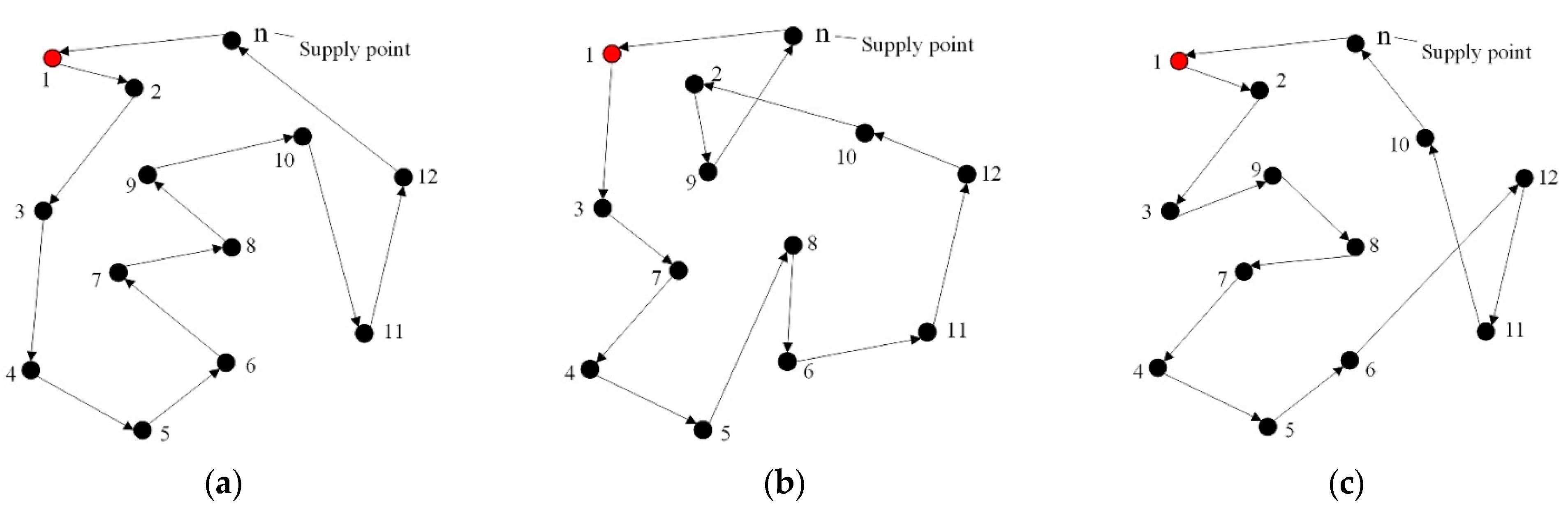
The research indicates that the transportation mode of FMS is basically the same as that of “Traveling Salesman Problem” (TSP), and the method of solving “TSP” is proposed to search for the optimal path. That is, if the middleman wants to reach “n” locations, he must choose the path he wants to take. Once the path is determined, he can only go through each location once, and finally he must return to the original departure location [21,22]. Figure 1 shows examples of different transportation paths under the sheep supply model of FMS. The goal of the path selection is to minimize the transportation distance. The key factors affecting cost and carbon emission are transportation distance, transportation time, and transportation capacity. Hypothesis: (1) Vehicle parameters are fixed values, which mainly focus on transportation distance and capacity. Transportation distance is closely related to the choice of transportation route, and the carrying capacity affects transportation cost and carbon emission between different supply points. (2) The location of supply points, the arrival time of vehicles and the number of sheep are known. (3) Meet the transportation time and the transportation distance in a positive correlation, regardless of the late penalty cost. (4) Acquire the sheep of each supply point according to the established route and satisfy the condition that the “TSP” problem path is closed loop.
2.1.2. Conceptual Framework
The investigation found that the transportation process of sheep can be divided into five stages: transportation preparation, loading, transportation, unloading, and temporary captivity. As shown in Figure 2, the participants in the transportation preparation stage are the seller and the transporter, the loading stage is completed by the loader, the transporter and the management department are involved in the transportation process, the unloading stage is completed by the unloader, and the temporary captivity stage is managed by the purchaser. Costs or energy consumption factors include vehicle preparation, tool preparation, quarantine, replenishment preparation, pharmaceutical preparation, loading equipment, limb collision, loading density, loading speed, road condition, vehicle speed, ventilation, transportation time, transportation distance, public management, unloading equipment, limb collision, unloading speed, site, feeding and drinking, pharmacology, etc. The main types of energy consumption are fuel consumption and energy consumption. The types of cost include depreciation of fixed assets, power cost, labor cost, management cost, maintenance and insurance cost, weight loss cost, and consumables cost.
2.2. Cost Accounting Method
2.2.1. Depreciation Cost of the Vehicle
The depreciation of vehicles refers to the loss of their own value caused by the decrease of vehicle conditions and the increase of operating costs during the use of vehicles [48,54]. Combined with the comprehensive impact of China’s national conditions and the economic benefits of vehicle operation, based on the straight-line depreciation method, the dynamic straight-line depreciation method is proposed [25,56]. That is, during the service life, based on the depreciation method without considering the value of time (linear depreciation method), a more practical depreciation method considering the value of time (dynamic linear depreciation method) is proposed. Then, according to the workload, the calculation method of vehicle depreciation cost of the current transportation is proposed:
where denotes the vehicle depreciation cost of the current transportation, CNY; is the purchase cost of the vehicle, CNY; is the residual value of the vehicle, CNY; is the service life of the vehicle, years; is the annual interest rate, %; is the estimated annual total carrying weight, kg/year; is the estimated annual transportation distance, km/year; is the current transportation distance, km; is the current transportation weight, kg.
2.2.2. Fuel Power Cost of the Vehicle
The mechanical equipment powered by internal combustion engine will produce energy consumption due to fuel combustion in use. And the fuel consumption can be calculated according to the basic parameters such as fuel consumption rate, vehicle speed and vehicle power. When the vehicle is running in a certain state, the fuel consumption rate equation of the engine can be derived according to the engine power corresponding to the vehicle speed and the fuel consumption of the vehicle running in 100 km [26,57]:
where denotes the fuel consumption rate, kg (kW h)−1; is the speed of the vehicle, km/h; is the fuel density, and the diesel density is generally 0.84 [57], kg L−1; represents the fuel consumption, L/100 km; is the running power of the engine, kW.
Then the fuel cost of the vehicle is
where denotes the fuel cost of the vehicle, CNY/(kg km); is the fuel price, CNY/L; is the full load fuel consumption rate, kg (kW h)−1; is the no-load fuel consumption rate, kg (kW h)−1; is the full load speed, km/h; is the no-load speed, km/h; is the rated power of the vehicle, kW; is the rated load capacity of the vehicle, kg.
According to the workload, the following calculation method of fuel cost for the current transportation is proposed:
where denotes the fuel cost of current transportation, CNY; is the number of sheep supply points; is the route length from supply point to supply point , km; is the number of deliveries from supply point to supply point ; is the average weight of each sheep, kg.
2.2.3. Depreciation Cost of the Tires
The depreciation cost of tires refers to the cost of outer tube, inner tube and cushion belt consumed by vehicle. According to relevant research, the consumption cost of tires cannot be ignored [47]. Referring to the calculation method of depreciation cost of fixed assets [25,56], the calculation method of tire depreciation cost of current transportation is proposed according to the workload:
where denotes the tire depreciation cost of the current transportation, CNY; is the purchase cost of tires, CNY; is the tire residual value, CNY; is the service life of tires, year; is the number of vehicle tires.
2.2.4. Maintenance and Insurance Cost of the Vehicle
Based on the analysis of relevant literature [25] and the conclusion of field investigation, the calculation method of vehicle maintenance and insurance cost for the current transportation is put forward according to the workload
where denotes the vehicle maintenance and insurance cost of the current transportation, CNY; and are the annual maintenance cost and insurance cost of vehicle respectively, CNY/year; and are annual maintenance cost coefficient and insurance cost coefficient of vehicle respectively; is the running time of vehicle, h/year.
2.2.5. Labor Cost in Transportation
Labor cost refers to the sum of direct and indirect labor costs incurred using labor force in the activities of production, operation and provision of labor services within a certain period [47]. For the labor cost of sheep transportation, only the direct labor cost incurred by the driver due to the use of labor in the current transportation is concerned—that is, the driver’s salary in the current transportation. According to the factors of labor cost in actual transportation, the calculation method of labor cost in transportation is proposed:
where denotes the driver’s salary for the current transportation, CNY; is the number of drivers; and are the basic wages (CNY/h) and working hours (h/day) of drivers respectively; is overtime pay after basic working hours (CNY/h); is the actual working time. Among them, is the loading time; is the unloading time; is the transportation time; is the rest time.
2.2.6. Operation and Management Cost of the Vehicle
Operation and management cost of the vehicle refers to the indirect operation cost related to vehicle ownership, usually including transportation management fee, tax and road maintenance fee, etc. [48]. According to the workload, the calculation method of operation and management cost of the current transportation is proposed:
where denotes the operation and management cost of the current transportation, CNY; is the different types of operation and management cost, CNY/year.
2.2.7. Labor Cost for Loading and Unloading
The survey found that the labor cost of loading and unloading is generally calculated according to the actual workload.
where denotes the loading or unloading costs, CNY; is the loading or unloading quantity; is the unit price of loading (unloading), CNY.
2.2.8. Weight Loss Cost of Sheep
Due to long-term transportation, long distance, bumps in the road, etc., the sheep will have different degrees of stress response and weight loss [58,59]. The following calculation method is proposed according to the actual transportation process:
where denotes the weight loss cost of the current transportation, CNY; is the average weight loss per 100 km after transportation, kg/100 km; is the expected price of sheep, CNY/kg.
2.2.9. Consumables Cost
According to field research and related research, feeding and pharmacological aids are sometimes arranged during the transportation to reduce the stress response and weight loss of sheep [58,59], and the following calculation method is proposed:
where is the total cost of consumables in the current transportation, including feed cost and pharmacological cost, CNY.
2.3. Carbon Emission Accounting Method
The carbon emission evaluation method proposed in this paper only aims at the carbon dioxide emission caused by the consumption of nonrenewable energy in the transportation process and takes the carbon dioxide emission weight as the measurement standard. The tracking study found that the energy consumption of vehicle fuel power is mainly involved in the transportation process of sheep, so this part only considers the carbon emission of vehicle fuel. The “top-down” method is adopted to calculate carbon dioxide emissions [60,61]:
where is carbon dioxide emission, kg; is the average cost of consumables per 100 km, CNY; is the factor of carbon dioxide emission, and the carbon dioxide emission factor of diesel is generally 3.16 [62], kg CO2/kg.
2.4. Objective Functions Analysis
2.4.1. Decision Variables
2.4.2. Objective Functions
- ①
- Objective Function of Cost:
- ②
- Objective Function of Carbon Emission:
The following constraints are met:
where Formulas (17) and (18) represent the objective function of cost and carbon emission respectively; Formula (19) represents that the transportation distance of vehicle from supply point to supply point is less than or equal to the total transportation distance of the current transportation; Formula (20) represents that the transportation weight of vehicle from supply point to supply point is less than or equal to the total mass of the current transportation. Formula (21) presents that the transportation weight does not exceed the rated weight of the vehicle ; Formula (22) represents the constraint on the transportation time, that is, the total work time is equal to the sum of the loading/unloading time, the transportation time, and the rest time. Formulas (23)–(25) indicates that the transportation tasks of each supply point are not separable and are transported by one vehicle. Formulas (26) and (27) represent the mutual constraint relationship between decision variables. Formula (28) indicates that the transportation path of the vehicle is a closed loop constraint condition; Formula (29) indicates that the value of decision variable is 0 or 1.
2.5. Solution Algorithm of the Model
- Step (a)
- Binary coding method is used to determine the chromosome length according to the number of supply points “n,” arrange the individuals according to the order of reaching the supply point, and generate the initial population. Set the operation parameters [38,40] of GA: the population size is generally taken as 20~100, the termination evolution algebra is generally taken as 100~500, the crossover probability is generally taken as 0.4~0.99, and the mutation probability is generally taken as 0.0001~0.1.
- Step (b)
- The fitness function of TSP problem is expressed by the reciprocal of the total distance of transportation route as follows:The distance from supply point to supply point is calculated according to the geographical coordinates of supply point, and the non-negative constant is set to prevent the fitness function from tending to 0 due to the excessive total distance of the path.
- Step (c)
- The fitness values are calibrated by formulas as follows [38]:where denotes the calibrated fitness value; denotes the original fitness value; denotes the upper bound of fitness function value; denotes the lower bound of fitness function value; denotes a positive real number in open interval (0,1). The calibrated fitness value can be enlarged or reduced according to the range of population change to prevent the supernormal individuals from dominating the group or the algorithm from swinging near the optimal solution.
- Step (d)
- The individual fitness value is calculated and sorted according to the size. Before the selection operation of GA, compare the individuals in the population one by one. If two individuals have similar genes (0 or 1) in similar positions, the number of the same genes is defined as similarity . Define the average fitness value as , take the average fitness value as the threshold value, and select the individuals whose fitness value is greater than the average fitness value to judge the similarity. When the similarity ( is the individual coding length), the two individuals are considered to have similarity [38].
- Step (e)
- Judge the degree of similarity of individuals in the population, the individuals with the highest fitness value are used as evolutionary templates to filter out similar individuals.
- Step (f)
- Repeat step (e). After each generation of the GA, select individuals with high fitness values as templates, and select individuals with different patterns to form new groups.
- Step (g)
- Determine whether the group size is reached. If yes, proceed to the next genetic operation such as crossover, mutation, etc.; otherwise repeat step (f). If the population size is not enough, the filtered individuals will make up for the missing population in the order of fitness value.
- Step (h)
- Judge whether the end requirement is satisfied, that is, whether the running algebra reaches the end evolutionary algebra. If not, go back to step (d). If yes, the distance from supply point to supply point and the total distance of the transportation path are decoded and output.
- Step (i)
- With and as intermediate variables, calculate the total target cost and various types of costs , , , , , , , and . Then calculate carbon emissions .
3. Results
3.1. Typical Case Analysis
According to “China Agricultural Statistics,” Liaoning Province has abundant resources of sheep and many farmers. However, most of the farmers are scattered in rural areas, and the scale of breeding is small. The average breeding scale of family farmers is less than 100. The suppliers involved in the supply chain generally have farmers, middlemen and slaughtering enterprises. The middlemen are generally local businessmen engaged in the sheep trading industry. They are involved in the supply of sheep and are responsible for liaising with farmers and slaughter enterprises. However, due to the lack of unified standard management, it shows the characteristics of high transportation cost and large energy consumption.
In this paper, 20 townships (towns) in Chaoyang City, Liaoning Province were selected as sheep supply points. ArcGIS10.2 was used to draw the geographical distribution map of 20 townships (towns) in Chaoyang City according to the scale of 1:1,000,000, the statistical results are shown in Table 1, and the mapping results are shown in Figure 3.
In order to quantitatively evaluate the cost and carbon emission of sheep transportation, it was necessary to analyze the values of the parameters first and assumed that the transportation vehicle will load 10 sheep on average at each supply point. As shown in Table 2, the basic parameter values involved in typical case are given. The values of the basic parameters were derived from references and field research and was not necessarily connected with the route of transportation. As shown in Table 3, the specific parameters of the random path, the suboptimal path, and the optimal path are given. The data was derived from field research and was related to the transportation path. Among them, the random path represents the irregular transportation route; the suboptimal path represents the transportation route close to the shortest total distance; the optimal path represents the transportation route of the shortest total distance. According to the data in Table 2 and Table 3, the specific values of cost and carbon emission under the three transportation routes can be calculated.
3.2. Performance Analysis of Path Optimization
In Matlab2018b software, GA coding rules were used to realize computer simulation analysis. For an optimization problem, the goal of computer simulation was to evolve a certain number of candidate solutions to a better solution. Set the operation parameters of GA: the number of individuals was 20, the population size was 30, the maximum genetic algebra was 10, 200 and 500, the crossover probability is 0.8, and the mutation probability was 0.09.
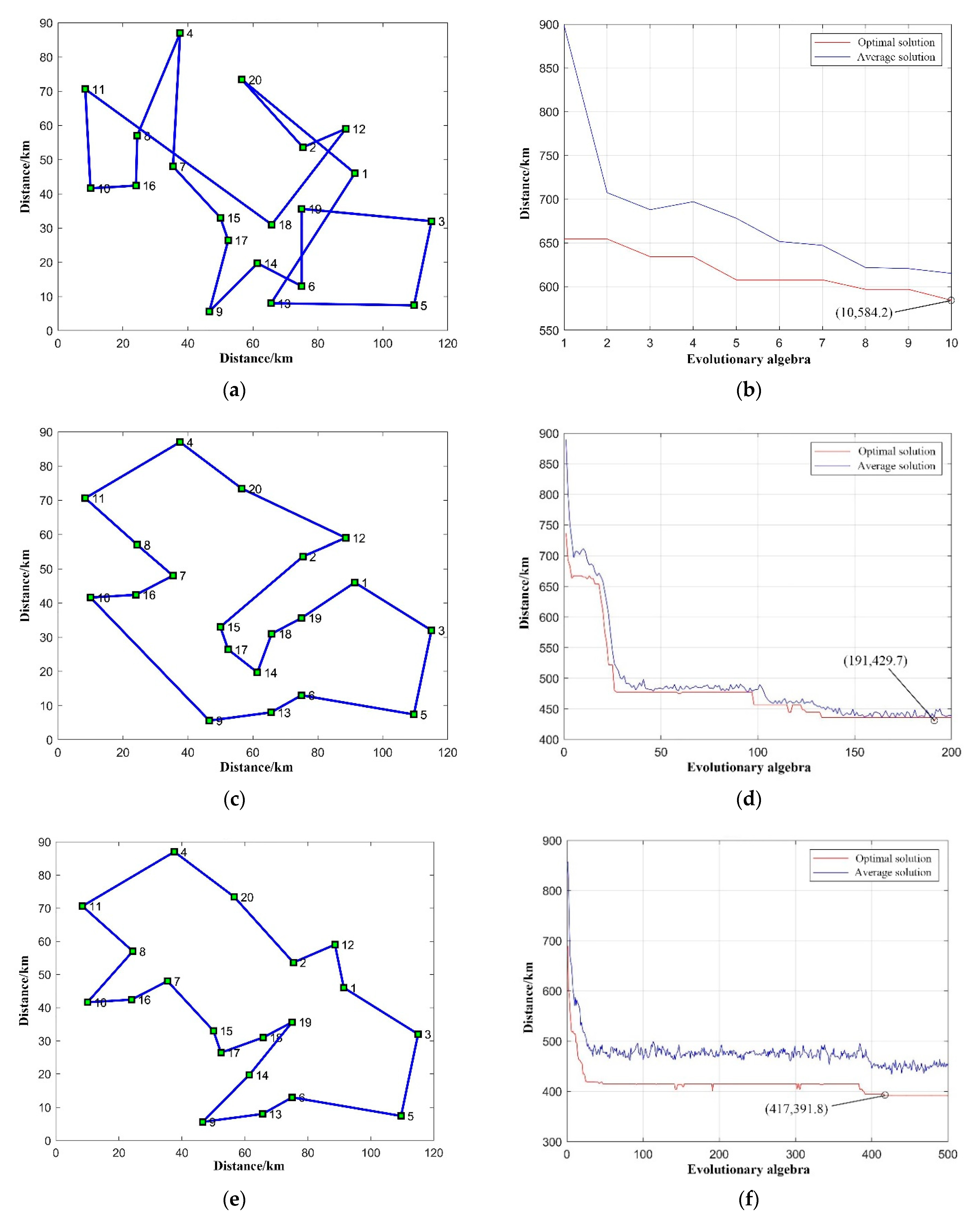
The process and results of path simulated in MATLAB2018b software are shown in Figure 4. Figure 4a,c,e shows the straight-line trajectories of the path simulation, and Figure 4b,d,f shows the search process of the average value and the optimal value of distance. Figure 4a,b shows the results of the GA simulation for 10 generations, which can be considered as a randomly generated path with a total simulated distance of 584.2 km; Figure 4c,d show the results of the GA simulation for 200 generations, but the optimal results are not achieved. It can be considered as a more optimized path, and the total simulated distance is 429.7 km. Figure 4e,f shows the results of the GA simulation for 500 generations, and the total simulated distance is 391.8 km.
In general, the maximum searching algebra of GA is 500 generations, and the optimal result after 500 generations will not be reduced in actual operation. Therefore, the results after 10 generations of GA simulation can be defined as random path, the results after 200 generations of GA simulation can be defined as suboptimal path, and the results after 500 generations of GA simulation can be defined as optimal path.
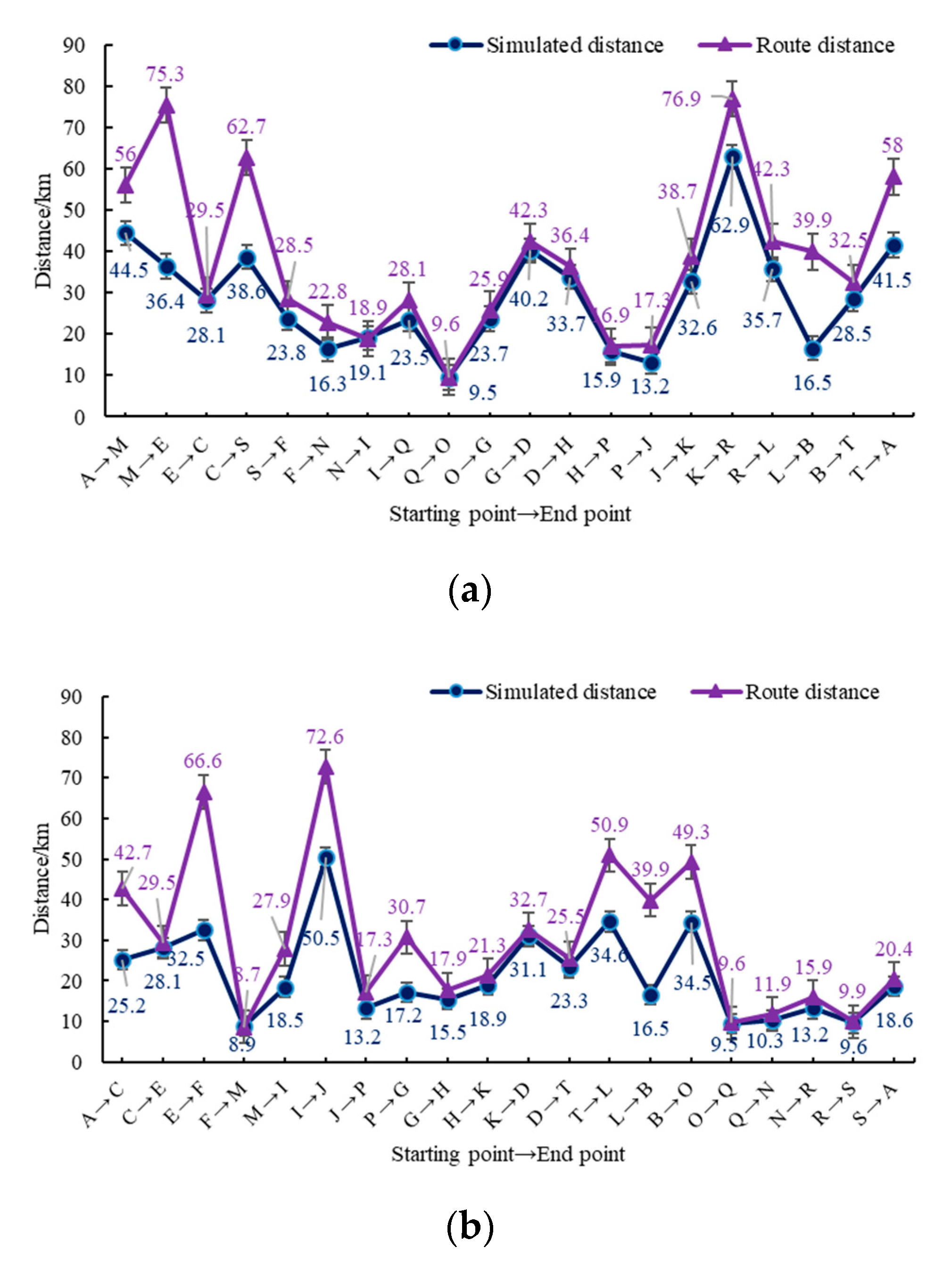
Generally, the distance of the actual route is greater than the straight-line distance, because the road is more tortuous due to the change of terrain or geographical environment. The simulated distance and route distance of random path, suboptimal path and optimal path are shown in Figure 5. The simulated distance represents the distance simulated by GA, and the route distance represents the actual distance between different supply points. The correlation coefficients between simulated distance and route distance of the three paths (random path, suboptimal path and optimal path) are 0.8722, 0.9041, and 0.7750 respectively, which shows that the simulated distance and route distance are highly correlated.
3.3. Performance Analysis of Cost and Emission Reduction
As mentioned above, the actual route distance is greater than the simulated distance (straight-line distance), so the calculation results of cost and carbon emission in this paper are based on the actual route distance, rather than the simulated distance.
As shown in Figure 6, they are the specific values and cost percentages of each type of costs in random path, suboptimal path, and optimal path, respectively. The cost types in the figure include fuel power cost of the vehicle, labor cost in transportation, maintenance and insurance costs of the vehicle, depreciation cost of the vehicle, labor cost of loading and unloading, weight loss cost of sheep, operation and management cost of the vehicle, tire depreciation cost of the vehicle, and consumables cost.
Comparing the cost percentages in Figure 6a–c, the cost distribution of different paths is basically the same. Among them, the vehicle fuel power cost of random path, suboptimal path and optimal path accounted for 27.1%, 23.2%, and 23.5%, respectively, and the consumables cost accounted for 14.6%, 12.5% and 12.6% respectively. In addition, the cost distribution of the optimal path is fuel power cost of the vehicle (23.5%), labor cost in transportation (15.3%), consumables cost (12.6%), maintenance and insurance cost of the vehicle (13.5%), depreciation cost of the vehicle (12.9%), labor cost for loading and unloading (10.0%), weight loss cost of sheep (5.1%), operation and management cost of the vehicle (3.7%), and depreciation cost of the tires (3.5%).
Comparing the cost values in Figure 6a–c, the cost of each type of optimal path is the lowest, the cost of each type of suboptimal path is slightly higher than that of optimal path, and the cost of each type of random path is the highest. Among them, the vehicle fuel power cost of random path, suboptimal path and optimal path are 1477 CNY, 1029 CNY, and 941 CNY respectively, which is the largest reduction of cost, followed by labor cost and consumables cost in transportation.
Regarding the carbon emission analysis, since the case is mainly related to the fuel consumption of the vehicle, the carbon dioxide emission of the fuel is the total carbon emission.
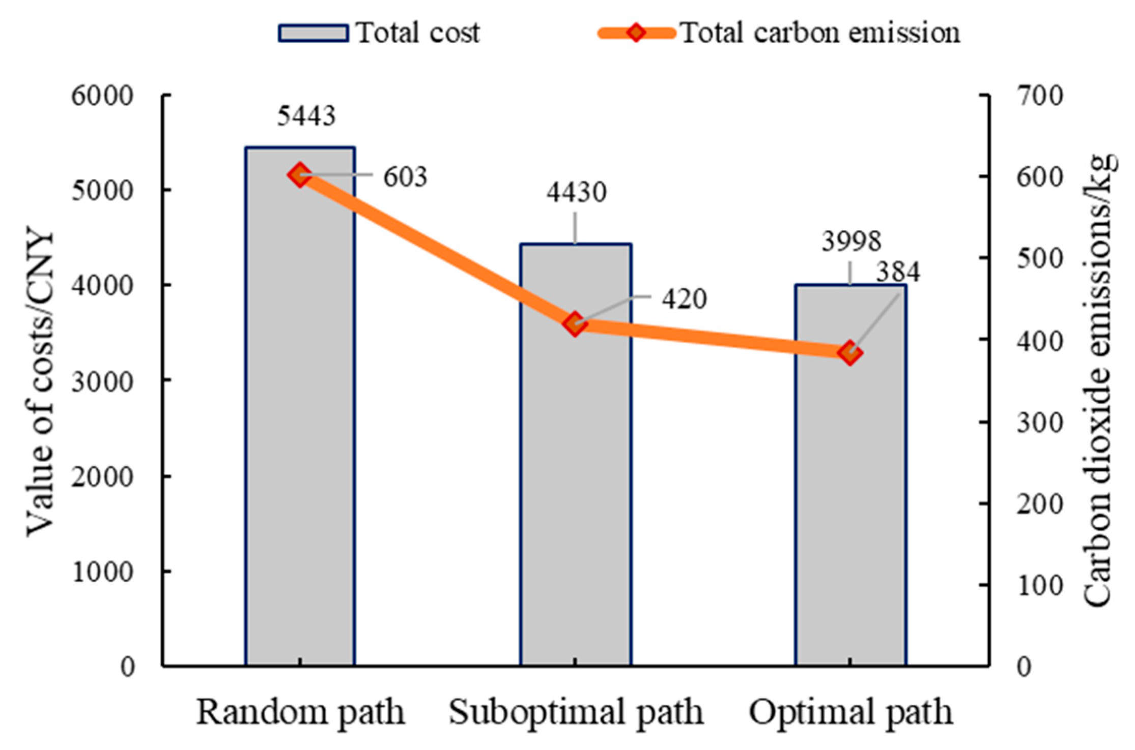
The total cost and total carbon emission of different transportation paths are shown in Figure 7, the total cost of the optimal path is 3998 CNY, which is 432 CNY less than the suboptimal path (reduced by 9.8%) and 1445 CNY less than the random path (reduced by 26.5%). The total carbon emission of the optimal path is 384 kg, which is 36 kg less than the suboptimal path (reduced by 8.6%) and 219 kg less than the random path (reduced by 36.3%).
4. Discussion
Based on the supply mode of FMS, through the investigation of typical cases, this paper concluded that the sheep transportation process can be divided into five stages, that is, transportation preparation stage, loading stage, transportation stage, unloading stage and captive stage. This is in accordance with the general steps of commodity transportation [25,47], but the difference is that living animals will produce different degrees of stress response after the end of transportation, which was mentioned by Schwartzkopf-Genswein et al. [11] and Miranda-de la Lama et al. [58] and generally need temporary captivity for a period of time to restore to the normal state.
For the different requirements of different industries, for instance, cold chain logistics has very strict requirements on transportation time [7]. The purpose is to prevent the deterioration of fresh commodities, while biomass raw material supply pays more attention to the transportation distance [8,25,26], and the location of supply points is often specially planned. Similarly, the transportation of farm commodity animals has its unique characteristics. Different from general cargo transportation, the sheep transportation usually has the characteristics of difficulty in control and uncertainty [63], and has to ensure animal health and animal welfare [10,11,12,58,59], this requires special care during transportation, such as pharmacological adjustment and reducing the weight loss of living body [11,58,63] (as shown in Table 3). Although the sheep transportation has its unique characteristics, it still conforms to the regularity of general cargo transportation, which needs to consider the transportation time, transportation distance, carrying capacity, fuel type, vehicle characteristics and the necessary insurance and maintenance of operating vehicles [2,4,15,57] (as shown in Table 2).
The investigation shows that under the supply model of FMS, more attention is paid to whether the transportation distance is the smallest and the requirements on the transportation time are not harsh. Therefore, this supply model conforms to the general regularity of TSP. The specific requirement is that the path selection goal is that the required path distance is the minimum value among all paths [21,22]. According to the literature analysis, intelligent algorithms [5,6,7,29,30] and dynamic programming method [18,31] can be used to comprehensively analyze and solve TSP. However, each method has certain limitations in application, so it is necessary to improve or construct a hybrid algorithm to solve TSP [30,32,33,34]. This study designed a model solving method based on the standard genetic algorithm. The solution algorithm was mainly improved in coding methods, fitness value calibration, adjustment of evolution algebra, adjustment of cross probability and adjustment of mutation probability [35,36,37,38,39,40] and is used to search for the optimal path of sheep transportation. As shown in Figure 4, the results of path optimization illustrated that when the range of crossover probability and mutation probability was set reasonably, and the maximum evolution algebra was set to 500 generations, the optimal solution can be found effectively. The optimal solution represented the optimal path and the shortest distance under the supply mode of FMS. The total distance of random path, suboptimal path and optimal path decreased in turn, and the evolution time was short, which proved that GA can quickly evolve to get better solution [35,36,37,38,39,40] (as shown in Figure 4). In addition, the distance of the actual route is greater than the straight-line distance (as shown in Figure 5), as the road is more tortuous due to the change of terrain or geographical environment. The correlation coefficients between simulated distance and route distance of three paths (random path, suboptimal path and optimal path) were all greater than 0.77, which showed that simulated distance and route distance have a high correlation. Therefore, the path optimization method proposed in this paper met the research reliability requirements.
Since the distance of actual route is usually greater than simulated distance (straight-line distance), so the results of the cost and carbon emission for this study were based on the distance of actual route. Comparing the cost percentages in Figure 6a–c, the cost distribution of different paths is basically the same, that is, the fuel power cost of the vehicle accounts for the largest proportion, followed by the labor cost in transportation, and the least is depreciation cost of the tires, which is basically consistent with the research results in literature [47]. The consumables cost and the sheep weight loss cost of the three paths account for about 20% of the total cost, indicating that a considerable part of the cost is generated while ensuring the animal health and animal welfare. But this cost is necessary, as described in literature [11] and literature [58], which guarantees both animal health and animal welfare, as well as meat quality.
After path optimization, the order of consumables cost in the cost distribution is changed, and the proportion of vehicle fuel power cost and consumables cost in the total cost is significantly reduced. The cost of each type of optimal path is the lowest, the cost of each type of suboptimal path is slightly higher than that of the optimal path, and the cost of each type of random path is the highest, among which the fuel power cost of vehicle is the largest, followed by the cost of labor and consumables in transportation. It showed that the cost of different types can be effectively reduced after path optimization, but the degree of reduction was different. The optimal path is the key to be explored in this study, and the results can be used as the best reference for the cost and carbon emission evaluation of sheep transportation.
5. Conclusions
From the perspective of cost and energy consumption reduction, through field investigation and theoretical analysis, this research evaluated the sustainability of FMS sheep supply model, which exits in various regions of China.
Under the typical case of the FMS supply model, this paper comprehensively analyzed the factors, sources, and types of cost and carbon emission in the transportation process of sheep, and a quantitative evaluation model was established. The GA was proposed to search for the optimal path of sheep transportation, and then the model solving algorithm was designed based on the basic GA.
The quantitative evaluation model established in this paper can systematically measure the cost and carbon emission generated in the process of sheep transportation, which can provide theoretical support and calculation basis for practical application. Since the transportation path is the most critical factor affecting the cost and carbon emission under the mode of FMS, this study chose to optimize the transportation path, which basically met the preliminary exploration of quantitative evaluation of the cost and carbon emission of sheep transportation.
In order to further strengthen the theoretical and practical exploration, we should combine the characteristics of model construction, optimization methods and parameter selection to establish evaluation methods under different transportation modes and finally achieve a more comprehensive analysis and evaluation of the development sustainability of sheep transportation industry.
Author Contributions
Conceptualization, M.Z., X.Z., and J.L.; methodology, M.Z.; software, M.Z.; validation, M.Z., H.F. and L.W.; formal analysis, M.Z.; investigation, M.Z., L.W., and X.Z.; resources, X.Z. and J.L.; data curation, M.Z. and L.W.; writing—original draft preparation, M.Z. and L.Z.; writing—review and editing, X.Z. and J.L.; visualization, M.Z.; supervision, X.Z.; project administration, X.Z. and J.L.; funding acquisition, X.Z. and J.L. All authors have read and agreed to the published version of the manuscript.
Funding
This research was supported by the National Modern Sheep Industry Technology System Project, grant number CARS-38 and the European Union Horizon 2020: Understanding food value chain and network dynamics, grant number 727243-2.
Conflicts of Interest
The authors declare no conflicts of interest.
References
- Li, Y.; Ukkusuri, S.V.; Fan, J. Managing congestion and emissions in transportation networks with dynamic carbon credit charge scheme. Comput. Oper. Res. 2018, 99, 90–108. [Google Scholar] [CrossRef]
- Chen, W.; Lei, Y. Path analysis of factors in energy-related CO2 emissions from Beijing’s transportation sector. Transp. Res. Part D Transp. Environ. 2017, 50, 473–487. [Google Scholar] [CrossRef]
- Trochu, J.; Chaabane, A.; Ouhimmou, M. A carbon-constrained stochastic model for eco-efficient reverse logistics network design under environmental regulations in the CRD industry. J. Clean. Prod. 2019, 245, 118818. [Google Scholar] [CrossRef]
- Gupta, P.; Mehlawat, M.K.; Aggarwal, U.; Charles, V. An integrated AHP-DEA multi-objective optimization model for sustainable transportation in mining industry. Resour. Policy 2018. [Google Scholar] [CrossRef]
- Yardimci, A.G.; Karpuz, C. Shortest path optimization of haul road design in underground mines using an evolutionary algorithm. Appl. Soft Comput. 2019, 83, 105668. [Google Scholar] [CrossRef]
- Dolgopolov, P.; Konstantinov, D.; Rybalchenko, L.; Muhitovs, R. Optimization of train routes based on neuro-fuzzy modeling and genetic algorithms. Procedia Comput. Sci. 2019, 149, 11–18. [Google Scholar] [CrossRef]
- Zhang, L.Y.; Tseng, M.L.; Wang, C.H.; Xiao, C.; Fei, T. Low-carbon cold chain logistics using ribonucleic acid-ant colony optimization algorithm. J. Clean. Prod. 2019, 233, 169–180. [Google Scholar] [CrossRef]
- Li, S.; Wang, Z.; Wang, X.; Zhang, D.; Liu, Y. Integrated optimization model of a biomass feedstock delivery problem with carbon emissions constraints and split loads. Comput. Ind. Eng. 2019, 137, 106013. [Google Scholar] [CrossRef]
- Park, C.; Lee, J.; Sohn, S.Y. Recommendation of feeder bus routes using neural network embedding-based optimization. Transp. Res. Part A Policy Pract. 2019, 126, 329–341. [Google Scholar] [CrossRef]
- Von Borell, E.; Schäffer, D. Legal requirements and assessment of stress and welfare during transportation and pre-slaughter handling of pigs. Livest. Prod. Sci. 2005, 97, 81–87. [Google Scholar] [CrossRef] [Green Version]
- Schwartzkopf-Genswein, K.S.; Faucitano, L.; Dadgar, S.; Shand, P.; González, L.A.; Crowe, T.G. Road transport of cattle, swine and poultry in North America and its impact on animal welfare, carcass and meat quality: A review. Meat Sci. 2012, 92, 227–243. [Google Scholar] [CrossRef] [PubMed]
- Caffrey, N.P.; Dohoo, I.R.; Cockram, M.S. Factors affecting mortality risk during transportation of broiler chickens for slaughter in Atlantic Canada. Prev. Vet. Med. 2017, 147, 199–208. [Google Scholar] [CrossRef] [PubMed]
- Bouchery, Y.; Fransoo, J. Cost, carbon emissions and modal shift in intermodal network design decisions. Int. J. Prod. Econ. 2015, 164, 388–399. [Google Scholar] [CrossRef]
- Lamba, K.; Singh, S.P.; Mishra, N. Integrated decisions for supplier selection and lot-sizing considering different carbon emission regulations in Big Data environment. Comput. Ind. Eng. 2019, 128, 1052–1062. [Google Scholar] [CrossRef]
- Resat, H.G.; Turkay, M. A discrete-continuous optimization approach for the design and operation of synchromodal transportation networks. Comput. Ind. Eng. 2019, 130, 512–525. [Google Scholar] [CrossRef]
- Sicilia, J.A.; Quemada, C.; Royo, B.; Escuín, D. An optimization algorithm for solving the rich vehicle routing problem based on Variable Neighborhood Search and Tabu Search metaheuristics. J. Comput. Appl. Math. 2016, 291, 468–477. [Google Scholar] [CrossRef]
- Bruglieri, M.; Mancini, S.; Pisacane, O. The green vehicle routing problem with capacitated alternative fuel stations. Comput. Oper. Res. 2019, 112, 104759. [Google Scholar] [CrossRef]
- Ozbaygin, G.; Savelsbergh, M. An iterative re-optimization framework for the dynamic vehicle routing problem with roaming delivery locations. Transp. Res. Part B Methodol. 2019, 128, 207–235. [Google Scholar] [CrossRef]
- Drexl, M.; Schneider, M. A survey of variants and extensions of the location-routing problem. Eur. J. Oper. Res. 2015, 241, 283–308. [Google Scholar] [CrossRef]
- Bargos, F.F.; de Queiroz Lamas, W.; Bargos, D.C.; Neto, M.B.; Pardal, P.C.P.M. Location problem method applied to sugar and ethanol mills location optimization. Renew. Sustain. Energy Rev. 2016, 65, 274–282. [Google Scholar] [CrossRef]
- Hui, W. Comparison of several intelligent algorithms for solving TSP problem in industrial engineering. Syst. Eng. Procedia 2012, 4, 226–235. [Google Scholar] [CrossRef] [Green Version]
- Chang, P.C.; Huang, W.H.; Ting, C.J. Dynamic diversity control in genetic algorithm for mining unsearched solution space in TSP problems. Expert Syst. Appl. 2010, 37, 1863–1878. [Google Scholar] [CrossRef]
- Dong, L.; Tong, X.; Li, X.; Zhou, J.; Wang, S.; Liu, B. Some developments and new insights of environmental problems and deep mining strategy for cleaner production in mines. J. Clean. Prod. 2019, 210, 1562–1578. [Google Scholar] [CrossRef]
- Hsiao, Y.H.; Chen, M.C.; Chin, C.L. Distribution planning for perishable foods in cold chains with quality concerns: Formulation and solution procedure. Trends Food Sci. Technol. 2017, 61, 80–93. [Google Scholar] [CrossRef]
- Sokhansanj, S.; Kumar, A.; Turhollow, A.F. Development and implementation of integrated biomass supply analysis and logistics model (IBSAL). Biomass Bioenergy 2006, 30, 838–847. [Google Scholar] [CrossRef]
- Yang, S.H.; Lei, T.Z.; He, X.F.; Li, Z.F.; Zhu, J.L. Study on economical radius of collected straw in biomass fuel cold compression molding. Trans. CSAE 2006, 22, 132–134. [Google Scholar]
- Layeb, S.B.; Jaoua, A.; Jbira, A.; Makhlouf, Y. A simulation-optimization approach for scheduling in stochastic freight transportation. Comput. Ind. Eng. 2018, 126, 99–110. [Google Scholar] [CrossRef]
- Lagoudis, I.N.; Shakri, A.R. A framework for measuring carbon emissions for inbound transportation and distribution networks. Res. Transp. Bus. Manag. 2015, 17, 53–64. [Google Scholar] [CrossRef] [Green Version]
- Zhang, Q.; Xiong, S. Routing optimization of emergency grain distribution vehicles using the immune ant colony optimization algorithm. Appl. Soft Comput. 2018, 71, 917–925. [Google Scholar] [CrossRef]
- Chen, J.; Shi, J. A multi-compartment vehicle routing problem with time windows for urban distribution—A comparison study on particle swarm optimization algorithms. Comput. Ind. Eng. 2019, 133, 95–106. [Google Scholar] [CrossRef]
- Wei, Y.; Avcı, C.; Liu, J.; Belezamo, B.; Aydın, N.; Li, P.T.; Zhou, X. Dynamic programming-based multi-vehicle longitudinal trajectory optimization with simplified car following models. Transp. Res. Part B Methodol. 2017, 106, 102–129. [Google Scholar] [CrossRef]
- Li, Y.; Soleimani, H.; Zohal, M. An improved ant colony optimization algorithm for the multi-depot green vehicle routing problem with multiple objectives. J. Clean. Prod. 2019, 227, 1161–1172. [Google Scholar] [CrossRef]
- Hu, H.; He, J.; He, X.; Yang, W.; Nie, J.; Ran, B. Emergency material scheduling optimization model and algorithms: A review. J. Traffic Transp. Eng. (Engl. Ed.) 2019, 6, 441–454. [Google Scholar] [CrossRef]
- Mosca, A.; Vidyarthi, N.; Satir, A. Integrated Transportation-Inventory Models: A Review. Oper. Res. Perspect. 2019, 6, 100101. [Google Scholar] [CrossRef]
- Mulloorakam, A.T.; Nidhiry, N.M. Combined Objective Optimization for Vehicle Routing Using Genetic Algorithm. Mater. Today Proc. 2019, 11, 891–902. [Google Scholar] [CrossRef]
- Xiao, Y.; Konak, A. A genetic algorithm with exact dynamic programming for the green vehicle routing & scheduling problem. J. Clean. Prod. 2017, 167, 1450–1463. [Google Scholar]
- Lin, C.; Choy, K.L.; Ho, G.T.; Ng, T.W. A genetic algorithm-based optimization model for supporting green transportation operations. Expert Syst. Appl. 2014, 41, 3284–3296. [Google Scholar] [CrossRef]
- Sivanandam, S.N.; Deepa, S.N. Introduction to Genetic Algorithms; Springer: Berlin/Heidelberg, Germany, 2008. [Google Scholar]
- Qiongbing, Z.; Lixin, D. A new crossover mechanism for genetic algorithms with variable-length chromosomes for path optimization problems. Expert Syst. Appl. 2016, 60, 183–189. [Google Scholar] [CrossRef]
- Karakatič, S.; Podgorelec, V. A survey of genetic algorithms for solving multi depot vehicle routing problem. Appl. Soft Comput. 2015, 27, 519–532. [Google Scholar] [CrossRef]
- Nakano, H. A Study on the Features of the Evolution Processes and Business Models of Global Enterprises in the Transport Sector. Transp. Res. Procedia 2017, 25, 3769–3788. [Google Scholar] [CrossRef]
- Zhang, Y.; Zhang, W.; Xu, W.; Li, H. A risk-reward model for the on-line leasing of depreciable equipment. Inf. Process. Lett. 2011, 111, 256–261. [Google Scholar] [CrossRef]
- Samaniego, R.M.; Sun, J.Y. Uncertainty, Depreciation and Industry Growth. Eur. Econ. Rev. 2019, 103314. [Google Scholar] [CrossRef]
- Jennergren, L.P. A note on the linear and annuity class of depreciation methods. Int. J. Prod. Econ. 2018, 204, 123–134. [Google Scholar] [CrossRef]
- Wang, T.; Lin, B. Fuel consumption in road transport: A comparative study of China and OECD countries. J. Clean. Prod. 2019, 206, 156–170. [Google Scholar] [CrossRef]
- Li, C.S.; Liu, C.C.; Peng, S.C. Bundled automobile insurance coverage and accidents. Accid. Anal. Prev. 2013, 50, 64–72. [Google Scholar] [CrossRef] [PubMed]
- Xu, M.Z.; Yu, G.Y.; Zhou, X.; Ge, X.L. Low-carbon vehicle scheduling problem and algorithm with minimum-comprehensive-cost. Comput. Integr. Manuf. Syst. 2015, 21, 1906–1914. [Google Scholar]
- Cheng, S.S.; Zhang, H.Z. Developing Models for Vehicle Depreciation &Interest Costs Estimation. J. Highw. Transp. Res. Dev. 2003, 4, 143–147. [Google Scholar]
- Maciej, H.; Jacek, Ż.; Grzegorz, F. Multiple Criteria Optimization of the Joint Vehicle and Transportation Jobs Selection and Vehicle Routing Problems for a Small Road Freight Transportation Fleet. Transp. Res. Procedia 2018, 30, 178–187. [Google Scholar]
- Tang, S.; Wang, W.; Cho, S.; Yan, H. Reducing emissions in transportation and inventory management: (R, Q) policy with considerations of carbon reduction. Eur. J. Oper. Res. 2018, 269, 327–340. [Google Scholar] [CrossRef]
- Li, H.; Lu, Y.; Zhang, J.; Wang, T. Trends in road freight transportation carbon dioxide emissions and policies in China. Energy Policy 2013, 57, 99–106. [Google Scholar] [CrossRef]
- Daryanto, Y.; Wee, H.M.; Astanti, R.D. Three-echelon supply chain model considering carbon emission and item deterioration. Transp. Res. Part E Logist. Transp. Rev. 2019, 122, 368–383. [Google Scholar] [CrossRef]
- Sarkar, B.; Ahmed, W.; Kim, N. Joint effects of variable carbon emission cost and multi-delay-in-payments under single-setup-multiple-delivery policy in a global sustainable supply chain. J. Clean. Prod. 2018, 185, 421–445. [Google Scholar] [CrossRef]
- Li, J.; Wang, D.; Zhang, J. Heterogeneous fixed fleet vehicle routing problem based on fuel and carbon emissions. J. Clean. Prod. 2018, 201, 896–908. [Google Scholar] [CrossRef]
- Labib, S.M.; Neema, M.N.; Rahaman, Z.; Patwary, S.H.; Shakil, S.H. Carbon dioxide emission and bio-capacity indexing for transportation activities: A methodological development in determining the sustainability of vehicular transportation systems. J. Environ. Manag. 2018, 223, 57–73. [Google Scholar] [CrossRef] [PubMed] [Green Version]
- Küpper, H.U.; Pedell, B. Which asset valuation and depreciation method should be used for regulated utilities? An analytical and simulation-based comparison. Util. Policy 2016, 40, 88–103. [Google Scholar] [CrossRef]
- Li, M.; Liu, L.; Li, Z.X. Relationship between Unit Consumption and Load Factor of Road transport vehicles. J. Highw. Transp. Res. Dev. 2013, 30, 141–146. [Google Scholar]
- Miranda-de la Lama, G.C.; Salazar-Sotelo, M.I.; Pérez-Linares, C.; Figueroa-Saavedra, F.; Villarroel, M.; Sañudo, C.; Maria, G.A. Effects of two transport systems on lamb welfare and meat quality. Meat Sci. 2012, 92, 554–561. [Google Scholar] [CrossRef]
- Llonch, P.; King, E.M.; Clarke, K.A.; Downes, J.M.; Green, L.E. A systematic review of animal based indicators of sheep welfare on farm, at market and during transport, and qualitative appraisal of their validity and feasibility for use in UK abattoirs. Vet. J. 2015, 206, 289–297. [Google Scholar] [CrossRef] [Green Version]
- Heinold, A.; Meisel, F. Emission rates of intermodal rail/road and road-only transportation in Europe: A comprehensive simulation study. Transp. Res. Part D Transp. Environ. 2018, 65, 421–437. [Google Scholar] [CrossRef]
- Zhang, L.; Long, R.; Chen, H.; Geng, J. A review of China’s road traffic carbon emissions. J. Clean. Prod. 2019, 207, 569–581. [Google Scholar] [CrossRef]
- Song, J.N.; Wu, Q.Q.; Yuan, C.W.; Zhang, S.; Bao, X.; Du, K. Spatial-Temporal Characteristics of China Transport Carbon Emissions Based on Geostatistical Analysis. Clim. Chang. Res. 2017, 13, 502–511. [Google Scholar]
- Santurtun, E.; Phillips, C.J.C. The impact of vehicle motion during transport on animal welfare. Res. Vet. Sci. 2015, 100, 303–308. [Google Scholar] [CrossRef] [PubMed]
Figure 1.
Examples of different transportation paths under the sheep supply model of FMS: (a) Path one; (b) Path two; (c) Path three.
Figure 1.
Examples of different transportation paths under the sheep supply model of FMS: (a) Path one; (b) Path two; (c) Path three.

Figure 2.
Flow chart of sheep transportation system: Numbers (1–7, a, b) indicate the corresponding relationship between different sources and types of cost or energy consumption.
Figure 2.
Flow chart of sheep transportation system: Numbers (1–7, a, b) indicate the corresponding relationship between different sources and types of cost or energy consumption.

Figure 3.
Geographical distribution map of 20 townships in Chaoyang City.

Figure 4.
Process and results of path simulation search: (a) simulation track of random path; (b) search process of random path distance; (c) simulation track of suboptimal path; (d) search process of suboptimal path distance; (e) simulation track of optimal path; (f) search process of optimal path distance.

Figure 5.
Simulation distance and route distance between supply points of different paths: (a) Simulated distance and route distance of random path; (b) Simulated distance and route distance of suboptimal path; (c) Simulated distance and route distance of optimal path.
Figure 5.
Simulation distance and route distance between supply points of different paths: (a) Simulated distance and route distance of random path; (b) Simulated distance and route distance of suboptimal path; (c) Simulated distance and route distance of optimal path.


Figure 6.
Costs and costs distribution of different paths: (a) Costs and its distribution of random path; (b) Costs and its distribution of suboptimal path; (c) Costs and its distribution of optimal path. Note: 1 Fuel power cost of the vehicle; 2 Labor cost in transportation; 3 Consumables cost; 4 Maintenance and insurance cost of the vehicle; 5 Depreciation cost of the vehicle; 6 Labor cost for loading and unloading; 7 Weight loss cost of sheep; 8 Operation and management cost of the vehicle; 9 Depreciation cost of the tires.

Figure 7.
Total cost and total carbon dioxide emissions of different paths.


Table 1.
Geographical coordinates of 20 townships in Chaoyang City.
| Serial Numbers | Township/Town Name | Longitude | Latitude |
|---|---|---|---|
| 1 | Lianhe Township (A) | 120.19° E | 41.53° N |
| 2 | Beigoumenzi Township (B) | 120.05° E | 41.60° N |
| 3 | Nanshuangmiao Township (C) | 120.41° E | 41.41° N |
| 4 | Jianping Town (D) | 119.71° E | 41.90° N |
| 5 | Yangshan Town (E) | 120.36° E | 41.19° N |
| 6 | Shengli Township (F) | 120.05° E | 41.24° N |
| 7 | Shenjing Town (G) | 119.69° E | 41.55° N |
| 8 | Xiaotang Town (H) | 119.59° E | 41.63° N |
| 9 | Xinglongzhuang Township (I) | 119.79° E | 41.17° N |
| 10 | Shahai Town (J) | 119.47° E | 41.49° N |
| 11 | Baishan Township (K) | 119.45° E | 41.76° N |
| 12 | Xiwujiazi Township (L) | 120.17° E | 41.65° N |
| 13 | Yangjiaogou Township (M) | 119.97° E | 41.19° N |
| 14 | Shuiquan Township (N) | 119.93° E | 41.29° N |
| 15 | Zhongsanjia Town (O) | 119.83° E | 41.42° N |
| 16 | Qingfengshan Township (P) | 119.59° E | 41.50° N |
| 17 | Gongyingzi Town (Q) | 119.85° E | 41.36° N |
| 18 | Polochi Town (R) | 119.97° E | 41.40° N |
| 19 | Dongdadao Township (S) | 120.05° E | 41.44° N |
| 20 | Qingsongling Township (T) | 119.89° E | 41.78° N |
Table 2.
Basic parameter values involved in typical case.
| Parameters | Values |
|---|---|
| Vehicle purchase cost/CNY | 166,000 |
| Vehicle residual value/CNY | 8300 (5%) |
| Vehicle service life/year | 10 |
| Annual interest rate/% | 1.75 |
| Annual carrying capacity/kg | 240,000 |
| Annual transportation distance/km | 20,000 |
| Full load power (60 km h−1)/kW | 70 |
| No-load power (80 km h−1)/kW | 65 |
| Full load speed/(km h−1) | 60 |
| No-load speed/(km h−1) | 80 |
| Vehicle rated power/kW | 118 |
| Vehicle rated load mass/kg | 7990 |
| Full load of 100 km fuel consumption/L | 40 |
| No load of 100 km fuel consumption/L | 26 |
| Fuel price/(CNY L−1) | 6.5 |
| The cost of single tire/CNY | 1600 |
| Residual value of single tire/CNY | 48 (3%) |
| Service life of tires/year | 2 |
| Number of tires | 6 |
| Vehicle maintenance cost factor/h−1 | 0.0002 |
| Vehicle insurance cost factor/year−1 | 0.03 |
| Vehicle annual running time/h | 400 |
Note: The data in the table comes from the field survey.
Table 3.
Specific parameters of different transportation paths.
| Parameters | Random Path | Suboptimal Path | Optimal Path |
|---|---|---|---|
| Total time/h | 30.5 | 23.5 | 23 |
| Loading time/h | 1.5 | 1.5 | 1.5 |
| Unloading time/h | 1.5 | 1.5 | 1.5 |
| Transportation time/h | 25.0 | 18.5 | 18 |
| Rest time/h | 2.5 | 2 | 2 |
| Current transportation distance/km | 758.5 | 601.2 | 512.9 |
| Current transportation mass/kg | 8000 | 8000 | 8000 |
| Carrying quantity | 200 | 200 | 200 |
| Loading (unloading) cost/CNY | 1 | 1 | 1 |
| Average weight loss per 100 km/kg | 0.02 | 0.02 | 0.02 |
| Live sheep price/(CNY kg−1) | 20 | 20 | 20 |
| Individual average mass/kg | 40 | 40 | 40 |
| Average consumption cost per 100 km/CNY | 1 | 1 | 1 |
| Basic wage/(CNY h−1) | 20 | 20 | 20 |
| Basic working time/ (h d−1) | 8 | 8 | 8 |
| Overtime wage/(CNY h−1) | 30 | 30 | 30 |
| Number of drivers | 2 | 2 | 2 |
Note: The data in the table comes from the field survey.
© 2020 by the authors. Licensee MDPI, Basel, Switzerland. This article is an open access article distributed under the terms and conditions of the Creative Commons Attribution (CC BY) license (http://creativecommons.org/licenses/by/4.0/).
Share and Cite
MDPI and ACS Style
Zhang, M.; Wang, L.; Feng, H.; Zhang, L.; Zhang, X.; Li, J. Modeling Method for Cost and Carbon Emission of Sheep Transportation Based on Path Optimization. Sustainability 2020, 12, 835. https://0-doi-org.brum.beds.ac.uk/10.3390/su12030835
AMA Style
Zhang M, Wang L, Feng H, Zhang L, Zhang X, Li J. Modeling Method for Cost and Carbon Emission of Sheep Transportation Based on Path Optimization. Sustainability. 2020; 12(3):835. https://0-doi-org.brum.beds.ac.uk/10.3390/su12030835
Chicago/Turabian StyleZhang, Mengjie, Lei Wang, Huanhuan Feng, Luwei Zhang, Xiaoshuan Zhang, and Jun Li. 2020. "Modeling Method for Cost and Carbon Emission of Sheep Transportation Based on Path Optimization" Sustainability 12, no. 3: 835. https://0-doi-org.brum.beds.ac.uk/10.3390/su12030835
Note that from the first issue of 2016, this journal uses article numbers instead of page numbers. See further details here.