Article

Mixed Logit Model Based on Improved Nonlinear Utility Functions: A Market Shares Solution Method of Different Railway Traffic Modes

1
School of Computer and Information Technology, Beijing Jiaotong University, Beijing 100044, China
2
Transportation and Economics Research Institute, China Academy of Railway Sciences, Beijing 100081, China
*
Author to whom correspondence should be addressed.
Sustainability 2020, 12(4), 1406; https://0-doi-org.brum.beds.ac.uk/10.3390/su12041406
Submission received: 13 December 2019 / Revised: 27 January 2020 / Accepted: 10 February 2020 / Published: 14 February 2020
(This article belongs to the Special Issue Sustainable Urban Transport Policy in the Context of New Mobility)

Abstract

:
In recent years, with the development of high-speed railway in China, the railway operating mileages and passenger transport capacity have increased rapidly. Due to the high density of trains and the limited capacity of railways, it is necessary to solve market shares of different railway traffic modes in order to adjust the operation plans appropriately and run railway passenger transport products in line with passenger demand. Therefore, the purpose of this paper is to calculate market shares by formulating a mixed logit model based on improved nonlinear utility functions taking different factors into consideration, such as seat grades, fares, running time, passenger income levels and so on. Firstly according to maximum likelihood estimation, the likelihood function of this mixed logit model is proposed to maximize utility of all passenger groups. After that, we propose two improved algorithms based on the simulated annealing algorithm (ISAA-CC and ISAA-SS) to estimate the unknown parameters and solve the optimal solution of this model in order to enhance the computational efficiency. Finally, a real-world instance with related data of Beijing–Tianjin corridor, is implemented to demonstrate the performance and effectiveness of the proposed approaches. In addition, by performing this numerical experiment and comparing these two improved algorithms with the traditional Newton method, the ant colony algorithm and the simulated annealing algorithm, we prove that the improved algorithms we developed are superior to others in the optimal solution.

1. Introduction

With the continuous improvement of railway networks, the connectivity across the regions has gradually increased, and passenger travel demand has increased with an unprecedented speed. However, due to the heavily congested passenger flow in peak hours in certain railway corridors, the passenger demand still cannot be satisfied even with the maximum departure frequency. To release the traffic pressure and solve the transportation problems, such as the mismatch between passenger demand and transportation resource allocation of different railway passenger service patterns, it is urgent to research the market shares of different railway traffic modes. Additionally, it directly affects the determination of the recent optimal train operation plans, e.g., the train capacity, departure quantity and departure frequency, and maximizes economic profits, social benefits and passenger demand. This research intends to explore these issues explicitly.

1.1. Literature Review

In the problem of discrete choice models, Train [1,2] developed a complete set of theoretical and empirical methods. Discrete choice models describe decision makers’ choices among alternatives. The decision maker can be people or any other decision-making unit. The alternatives might represent competing products or any other options over which choices must be made. To fit a discrete choice framework, the set of alternatives, called the choice set, needs to exhibit three characteristics. First, the alternatives must be mutually exclusive from the decision maker’s perspective. Choosing one alternative necessarily implies not choosing any of the other alternatives. The decision maker chooses only one alternative from the choice set. Second, the choice set must be exhaustive to ensure all possible alternatives are included. The decision maker chooses one of the alternatives. Third, the number of alternatives must be finite and the researcher must be able to count the alternatives. Discrete choice models are usually derived under the utility-maximizing assumption. Marschak [3] provided a derivation from utility maximization. Following Marschak, models that can be derived in this way are called random utility models (RUMs). Therefore in the traffic field, they are used for predicting transfer passenger demand and calculating market shares of different traffic modes.
Most time series models are easier to implement than discrete choice models, but the former are limited because they do not explain how different passengers make decisions, while discrete choice models and regression models are distinguished by saying that regressions examine choices of ’how much’ and discrete choice models examine choices of ’which’ and ’how much’. For example, Train et al. [4] analyzed the number and duration of phone calls that households made. In their experiments, the reason why they chose a discrete choice model instead of a regression model is that it allows greater flexibility in handling the nonlinear price schedules. In general, the researcher needs to consider the goals of the research and the capabilities of alternative methods when deciding whether to apply a discrete choice model.
The most prominent types of discrete choice model, namely logit models and probit models, are introduced and compared briefly here. It is important to note that the flexibility of the probit model in handling correlations over alternatives and time is its main advantage. Its only functional limitation arises from its reliance on normal distribution, because in some situations unobserved factors may not be normally distributed. For example, the multinomial probit (MNP) model is highly flexible but its application is limited due to the complexity and high computation demand of the model.
By far the most widely used discrete choice model is logit. Its popularity is due to the fact that the formula for the choice probabilities takes a closed form and is readily interpretable. There are some improved models of the logit model as follows.
The multinomial logit (MNL) model is the most commonly used in practice, with the advantages of simplicity, reliability, and easy implementation. It is a generalization of the binary logit model and is used to describe how an individual chooses among three or more discrete alternatives [5]. In this model, there is an important assumption about the characteristics of choice probabilities, which means the probability ratio of two alternatives is unaffected by the systematic utilities of any other alternatives. However, the MNL model also has some inherent theoretic defects, which led to the need for more refined models.
In order to overcome the restriction of MNL model, Nested logit (NL) model is first proposed [6] as an extension of MNL model just a few years after MNL model. Similar to the MNL model, NL model is a choice model that is used to predict the probability that an individual will select one alternative out of a set of mutually exclusive and collectively exhaustive alternatives. Both MNL and NL models are based on random utility theory, but differ in how they represent substitution patterns among alternatives. The NL model represents a partial relation of the independence of identically distributed (IID) and independence from irrelevant alternatives (IIA) assumptions of the MNL model (Hensher et al. [7]). NL model partitions the choice set into several sub-nests and puts alternatives which are similar and maybe correlate with each other in the same sub-nest. The correlation among alternatives within each sub-nest can be captured. However, no correlation across nests can be depicted. When alternatives can not be partitioned into well separated nests to reflect their correlations, the NL model is not appropriate. Cross-nested logit (CNL) model is a direct extension of the NL model, where each alternative may belong to more than one nest. The correlation across nests can be estimated using the CNL model.
Mixed multinomial logit (MMNL) model (McFadden et al. [8]) offers significant advantages over the MNL model by allowing for random taste variation across decision makers. MMNL model not only allows for random taste variation, but also in principle avoids the unrealistic MNL substitution patterns resulting from the independence from irrelevant alternatives (IIA) assumption, which dictates that the dependency between any two alternatives is the same across alternatives, making the MNL model an inappropriate choice in many scenarios. The biggest drawback of the MMNL model is the fact that the integrals representing the choice probabilities do not have a closed-form expression and need to be approximated through simulation (Train [1]; Hess et al. [9]). A second issue with the MMNL model is the choice of distribution to be used for the random taste coefficients, especially in the case where an a priori assumption exists about the sign of a given coefficient (Hensher et al. [10]; Hess et al. [11]; Hess et al. [12]).
Mixed logit (MXL) model is suitable for handling random preferences, random coefficients, and some kinds of correlation problems, such as correlation among alternatives, and it allows the unobserved factors to follow any distribution. See Section 2.2.1 for details.
To the best of our knowledge, the majority of existing literature which research the logit models based on different utility functions, devotes to some objectives such as maximizing the utility values of passengers and estimating the coefficients of influence factors. For comparative convenience, we list the detailed characteristics of some closely related references in Table 1, including traffic modes, variables in utility functions and formulated models. The key to solve the model is to analyze the variables involved in the objects and utility functions of traffic modes.

1.2. The Focus of This Paper

As mentioned above, there are some unsolved problems of many studies in the existing literature as follows. Firstly, there is no researcher who studies the market shares of different railway traffic modes standing fom the passengers’ points of view and who also analyzes which type has higher market share and higher operational revenue standing from the enterprise’s point of view. Then, many studies have explored passenger demand predicting approaches by logit models, in which the main focus is to establish utility functions in a linear way but without considering that there is not a fixed relationship between the value of utility and passenger income about different traffic modes. Last but not least, nowadays, the main focus of recent research in Table 1 is how to reasonably and comprehensively choose the variables involved in the models when studying the influencing factors of different traffic modes. The number of variables involved in each reference is relatively small, so some traditional software, such as SPSS or ALOGIT, and traditional methods, such as the Newton method (Appendix A) or its deformations (ramped Newton method), can usually be used to estimate unknown parameters and solve the optimal solution of the functions. Nevertheless, using the Newton method to solve the problems, the time complexity is large and it may lead to non-convergence of the results.
In summary, specifically, the detailed contributions of this paper are summarized as follows.
(a) According to different products of railway passenger transportation, we consider different seat grades, fares, running time and train number for different railway traffic modes.
(b) It is common knowledge that passenger income is one of the most important factors affecting the travel intention of passengers to choose transfer vehicles; and the time value of passengers at different income levels are different. So in this paper, considering that there is a certain function relationship between the utility value and the income level and it is obviously unreasonable to formulate passenger income functions directly into linear utility functions, we establish different nonlinear utility functions which are mainly including different passenger income functions for different traffic modes.
(c) The model established in this paper involves 48 variables including passenger income, travel time, travel expense and so on. Therefore, some representative heuristic algorithms such as the ant colony algorithm and the simulated annealing algorithm are chosen to solve this problem; and according to their current problems, we also develop two improved algorithms based on the simulated annealing algorithm (ISAA-CC and ISAA-SS) to estimate unknown parameters of the utility functions; and then running time, optimal solution and convergence speed of these improved algorithms are compared with those of the Newton method, the ant colony algorithm and the simulated annealing algorithm. The results show that these two improved algorithms in this paper are better than others, obviously.
The rest of this paper is organized as follows. In Section 2, a mixed logit model based on improved nonlinear utility functions is rigorously formulated to solve the market shares; and to reduce computational complexity, we adopt maximum likelihood estimation to construct a corresponding likelihood function. Then, Section 3 develops two improved algorithms based on the simulated annealing algorithm (ISAA-CC and ISAA-SS) to solve the problem in this paper. Next, we also design one case to demonstrate the effectiveness of the proposed approaches in Section 4. Finally, some conclusions and further studies are presented in Section 5.

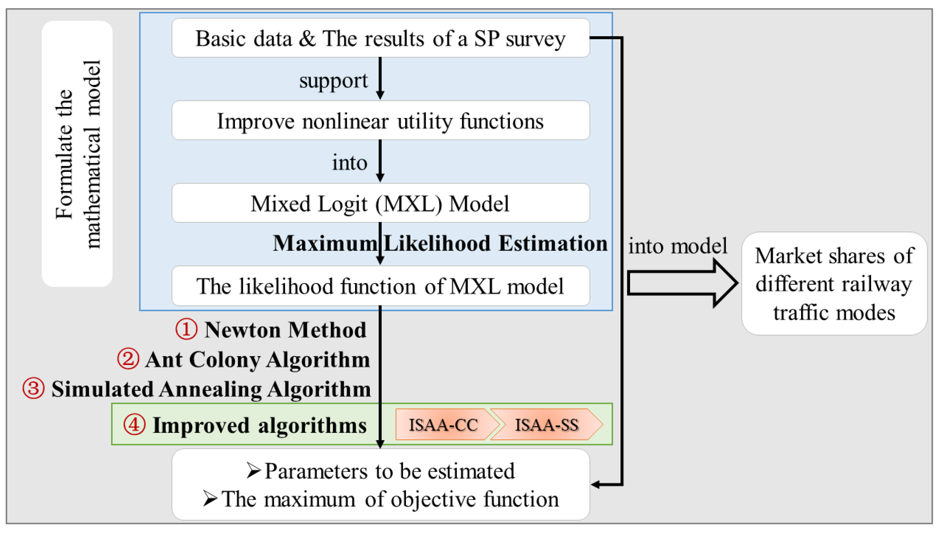
2. Mathematical Formulation

To characterize this problem in a mathematical way, in this section, we will explicitly discuss the formulation process for a mathematical model about solving market shares of different railway traffic modes, namely mixed logit model based on improved nonlinear utility functions. The technical route of the specific research in this paper is shown in Figure 1.
It can be seen in the figure that modeling technique in this paper is the part of blue bottom, including improved nonlinear utility functions, a mixed logit model, a likelihood function and their relationships. The utility functions are substituted into the logit model and we adopt maximum likelihood estimation to construct a corresponding likelihood function.

2.1. Problem Description

Firstly, according to the ’per capita disposable income of urban residents’ of the National Bureau of Statistics in China, we divided all railway passengers into three passenger groups with different income levels, i.e., low-income passenger group whose income is less than RMB 3000 in a month, medium-income passenger group whose income is between RMB 3000 and RMB 8000 in a month and high-income passenger group whose income is larger than RMB 8000 in a month.
Generally speaking, the choices of different passenger groups for traveling are closely related to the service attributes of railway traffic modes, which have inherent regularity and functional relationship. Then, in this paper, due to facilitate calculation and comprehensive coverage, the service attributes are taken as the main indicators of passenger travel behaviors, including rapidity, economy, comfort, safety and convenience.
(a) Rapidity is quantified by the value of passengers travel time and directly related to passenger income.
(b) Economic is quantified by travel expense of passengers, such as ticket prices.
(c) Comfort is including the space, service and environment of railway traffic modes, which are measured by fatigue recovery time of passengers and different grades of train seats (reflected by the change of ticket prices). Therefore, the comfort degree is inversely proportional to travel time and proportional to travel expense, as shown in Figure 2 below.
On the one hand, with the same travel expense, the less travel time is, the higher comfort degree will be. However, with the increase of travel time, the increment of comfort degree caused by saving unit time will decrease. On the other hand, with the same travel time, the higher travel expense (which means the higher seat grade) is, the higher comfort degree will be. However, with the increase of travel expense, the increment of comfort degree caused by raising unit expense will decrease.
(d) Convenience is quantified by the value of total time, including boarding time, departure time and waiting time.
(e) Safety is quantified by the accident rate of traffic modes, that is the safety guarantee of life, health and financial of passengers.
Since we discuss the railway traffic modes, we can conclude that the safety and convenience of each railway train have little difference. Finally base on this, in order to truly reflect the passenger flow characteristics of railway in China, the authors conducted a Stated Preference (SP) survey and a total of 717 valid questionnaires have been collected. The survey results of passenger travel considerations analysis are shown in Table 2.
The results show that, 453 passengers think that rapidity is their primary consideration, accounting for 63.18% of the total passengers, 111 passengers think that economy is their primary consideration, accounting for 15.48%, and 153 passengers think that comfort is their primary consideration, accounting for 21.34%.
Before the model is established in this paper, the following assumptions are made in order to formulate the problem.
(A1)
According to the utility theory proposed by Fishburn [24], based on the usual mentality of passengers for making choices, passengers will evaluate the utility values of different available railway traffic modes and always choose the most reasonable mode which has maximum utility value.
(A2)
Under the condition of assumption (A1) and in order to the convenience of research, we will take the same income passenger group as a whole.
All the involved parameters and variables are listed below (Table 3) for the convenience of formulating the problem under consideration.

2.2. Mathematical Model

In addition to these primary service attributes, the income level of passengers also indirectly determines their travel intention to a large extent. Therefore, in order to make the model much closer to the actual case, this paper not only considers three service attributes including rapidity, economy and comfort, but also adds passenger income to construct utility functions. See Section 2.2.2 for details.

2.2.1. Mixed Logit Model

In this paper, we adopt the mixed logit (MXL) model (McFadden, et al. [8], Hensher, et al. [10] and Train [1]) to solve the market shares according to Section 1.1, which can be derived from random utility theory and can approximate any discrete choice models by making the following definitions.
(a) There is a set of available alternatives (railway traffic modes, M) and a set of individuals (passenger groups with different income, Q).
(b) There is a set of measured attributes X of the individuals and their alternatives.
(c) According to assumption (A1), i.e., the maximization of utility, the individual q selects the alternative m which maximizes their personal utility, i.e., U m q > U l q , m l M , q Q , subject to their individual constraints. The value of utility itself is based on a comparison and individual evaluation of the different characteristics which describe the attractivity of the alternatives.
(d) It is not possible to possess complete information about all elements that determine this choice. Errors can arise for observational reasons. For example, instead of the true modal characteristic X , only X (or a functional f ( X ) may be available. To take into account the unobserved measurement error, X is effectively replaced by X + ε or f ( X ) + ε , where ε designates the unknown error.
For individuals who have the same set of alternatives and face the same constraints, it can be assumed that the residual ε is random variable with mean 0 and a certain distribution.
More precisely in this paper, a utility U m q can be represented by two components, i.e., an observed representative component V m q which is a function of measured mode-specific and socioeconomic attributes X, and an unknown random component ε m q which represents unobserved attributes, taste variations, and measurement or observational errors.
The utility U m q = V m q + ε m q is random across the individuals, this event is associated with a probability, i.e.,
P m q = P { U m q > U l q , m l M , q Q } ,
or more explicitly, i.e.,
P m q = P { ε l q ε m q + V m q V l q , m l M , q Q } .
This means that the probability of passenger group q choosing mode m equals the probability that the utility of choosing m is greater than that of any other choices. For MXL model, each error ε m q is assumed to be independently and identically distributed over the population and for each individual according to the Gumbel extreme value distribution which has the following cumulative distribution function with variance δ 2 , i.e.,
P { ε m q ε } = exp exp π 2 6 · δ 2 · ε .
So the distribution function about the difference between two random errors ε m l q = ε m q ε l q is
F ( ε m l q ) = exp ε m l q 1 + exp ε m l q .
The probability that passenger group q chooses railway traffic mode m can now be expressed as follows.
P m q = 1 l m M exp ( V m q V l q ) = exp V m q l m M exp V l q .

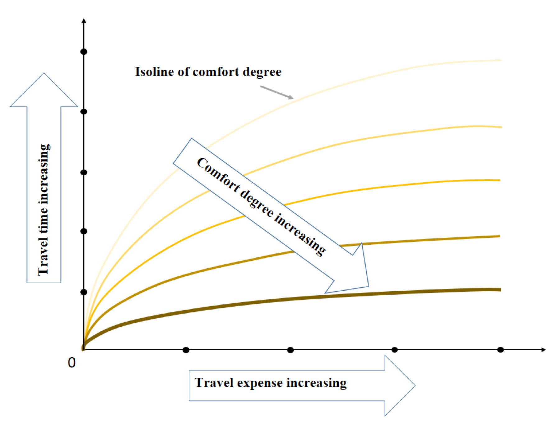
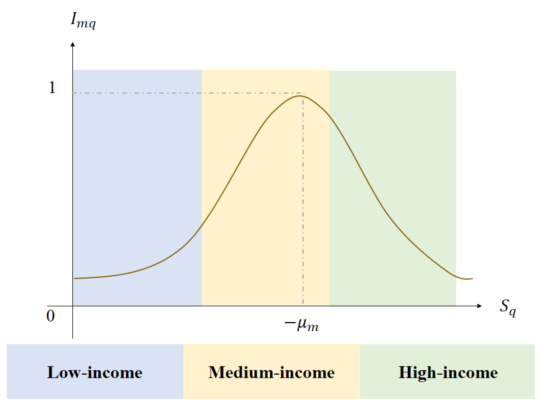
2.2.2. Improved Nonlinear Utility Functions

As discussed in previous parts, the authors decide to use not only three service attributes including rapidity, economy and comfort, but also ’passenger income’ attribute. Because the units of time and expense are not uniform and the dimensions are different, it can not be calculated in one function. So we introduce ’time value’ attribute to replace ’travel time’ in order to unify their dimensions. According to the research of Wardman [25] on the time value, they believe that the marginal utility of time increases with income. Different income levels of passenger groups have different unit time values which will be denoted by v ( t ) q , q Q . Generally speaking, the time value of high-income passenger group is higher than that of low-income passenger group and medium-income group. Therefore based on the above analysis, we establish improved nonlinear utility functions for different railway traffic modes according to different passenger income levels. The utility value of passenger group q who choose railway traffic mode m expressed by the following function, i.e.,
V m q = α m 1 · R m q + α m 2 · s S E m s + α m 3 · s S C m s q + α m 4 · I m q , m M , q Q .
Among them, a utility function above include several functions as follows.
(a) v ( t ) q = s q / ( 30 · 24 ) denotes the unit (hour) time value of passenger group q.
(b) T m s = T max / ( 1 + β m s · exp ( γ m s · t m ) ) denotes fatigue recovery time of passengers. The minimum time of fatigue recovery is T min = T max / ( 1 + γ m s ) where t m = 0 because fatigue recovery time is related to travel time, the types of railway traffic modes and the degrees of seats.
(c) R m q = t m · v ( t ) q denotes rapidity function about passenger group q who choose railway traffic mode m because rapidity of railway traffic modes is inversely proportional to the time value spent by passengers.
(d) E m s = e m s denotes economy function about passenger group q who choose railway traffic mode m seat s because economy of railway traffic modes is inversely proportional to travel expense spent by passengers.
(e) C m s q = T m s · v ( t ) q denotes comfort function about passenger group q who choose railway traffic mode m seat s.
(f) I m q denotes passenger income function about passenger group q who choose railway traffic mode m. Under the condition of assumption (A1), the complex relations between different passenger income levels and the utility values of choosing different railway traffic modes are as follows. When passenger income is in a certain range, the utility value is the highest and when the income is lower or higher, the utility value will decrease. So the passenger income function should be established as curve which can map variables by probability density function of Normal distribution or Gaussian distribution. We establish passenger income function as follows whose graph is shown in Figure 3.
I m q = 1 2 π · σ m q · exp S q μ m q 2 π · σ m q 2 .
Then, in the next subsection, each improved nonlinear utility function of railway traffic modes will be substituted into the mixed logit model established in this paper; and to reduce the difficulty of solving this complex mixed logit model, we adopt maximum likelihood estimation to construct a corresponding likelihood function.

2.2.3. Maximum Likelihood Estimation

The purpose of this study is to maximize utility of all passenger groups in this mixed logit model; and we need to estimate the values of unknown parameters in the model. Maximum likelihood estimation is often applied for the estimation of this mixed logit model because the likelihood function is concave and can be constructed as follows under a suitable condition. Therefore, we can obtain a unique solution, i.e., the maximum value of the likelihood function.
For a random sample of size M, the likelihood function can be viewed as the product of choice probabilities associated with Q subsets of independent observations, in which the first subset includes q = 1 individuals observed to have chosen alternatives 1 m 1 , the next one q = 2 individuals observed to have chosen alternatives m 1 + 1 m 1 + m 2 , etc. That is
ϕ = m = 1 m 1 P m 1 · m = m 1 + 1 m 1 + m 2 P m 2 m = m 1 + m 2 + + 1 M P m Q .
Then, in this study, we introduce 0-1 variables y m q where m M and q Q , as selection indicators for selection of different passenger groups, i.e.,
y m q = 1 passenger group q chooses railway traffic mode m , 0 otherwise ,
and m M y m q = 1 , q Q .
Due to that each passenger group can only choose one railway traffic mode and all passenger groups are independent, the expression of ϕ can be simplified by y m q as follows,
ϕ = q Q m M P m q y m q .
Because ln ϕ is the monotone increasing function of ϕ , ln ϕ and ϕ have the same extreme point. In order to solve this mixed logit model conveniently, the corresponding log-likelihood function can now be written as follows.
ϕ = ln ϕ = q Q m M y m q · ln P m q = q Q m M y m q · V m q ln m M exp ( V m q ) .
In this paper, the optimization objective is to maximize the log-likelihood function above. Therefore, in a word, the mixed logit model based on the improved nonlinear utility functions is shown as follows.
max ϕ = ln ϕ = q Q m M y m q · ln P m q = q Q m M y m q · V m q ln m M exp ( V m q ) ,
where V m q = α m 1 · R m q + α m 2 · s S E m s + α m 3 · s S C m s q + α m 4 · I m q , m M , q Q , R m q = t m · v ( t ) q = t m · d q 30 · 24 , m M , q Q , E m s = e m s , m M , s S , C m s q = T m s · v ( t ) q = T max 1 + β m s · exp ( γ m s · t m ) · d q 30 · 24 , m M , q Q , s S , and I m q = 1 2 π · σ m q · exp S q μ m q 2 π · σ m q 2 , m M , q Q . s.t. α m 1 + α m 2 + α m 3 + α m 4 = 1 , 0 < α m 1 < 1 , 0 < α m 2 < 1 , 0 < α m 3 < 1 , 0 < α m 4 < 1 , m M , y m q { 0 , 1 } , m M , q Q .
The likelihood estimator is
θ ^ = argmax θ R ϕ ( θ ) = θ 1 ^ θ 2 ^ θ 3 ^ θ 8 ^ = α 11 ^ α 21 ^ α 31 ^ α 81 ^ α 12 ^ α 22 ^ α 32 ^ α 82 ^ α 13 ^ α 23 ^ α 33 ^ α 83 ^ α 14 ^ α 24 ^ α 34 ^ α 84 ^ μ 1 ^ μ 2 ^ μ 3 ^ μ 8 ^ σ 1 ^ σ 2 ^ σ 3 ^ σ 8 ^
of this objective function ϕ ( θ ) , which denotes a vector of unknown parameters to be estimated in eight utility functions, can be obtained in next section.

3. Solution Approaches

In this section, we aim to introduce two traditional heuristic algorithms, i.e., the ant colony algorithm and the simulated annealing algorithm, and then develop two improved Algorithms 1 and 2 based on the simulated annealing algorithm (ISAA-CC and ISAA-SS), to solve the problem in this paper and to obtain the maximum of the objective function, i.e., ϕ ( θ ) and the unknown parameter to be estimated, i.e., θ ^ = θ 1 ^ θ 2 ^ θ 3 ^ θ 8 ^ in short time, efficiently; and we also compare the performance of these algorithms with the Newton method according to a real numerical experiment in next section.
Algorithm 1: A heuristic bionic evolutionary algorithm based on swarm intelligence.
Step 1. The relevant parameters need to be initialized, including ant colony size (the total
  number of ants) a n t _ m a x , the pheromones volatilization coefficient ρ , total pheromones
  released by ants for one iteration Q (constant), a constant of transfer probability p 0 , maximum
  number of iterations i t e r _ m a x . Initial pheromones τ t ( 0 ) = ϕ ( θ ) .
Step 2. Do for i = 1, 2, ⋯, i t e r _ m a x ,
Step 2.1. Do for t = 1, 2, ⋯, a n t _ m a x ,
Step 2.1.1. Each ant is randomly placed in different positions, and the next position of ant t,
  namely next feasible solution, is determined according to transfer probability p t , i.e.,
p t = max s [ 1 , a n t _ m a x ] τ s ( i ) τ t ( i ) max s [ 1 , a n t _ m a x ] τ s ( i ) .
Step 2.1.2. According to following judgement, iterative formula of parameter to be estimated is
θ ( i + 1 ) = θ ( i ) + r a n d · λ p t < p 0 , θ ( i ) + r a n d · u p p e r l o w e r 2 p t < p 0 .
 (a) Local Search: If the pheromones of ant t is closer to the highest concentration of
  pheromones in the current population (i.e. the current maximum of the function), the transfer
  probability p t is smaller, and variable value θ tends to be fine-tuning, i.e.,
   θ ( i + 1 ) = θ ( i ) + r a n d · λ where r a n d is a 0-1 random number, and λ = 1 / ( t + 1 ) is heuristic
  function (degree of expectation) and it gradually decreases as the iteration progresses.
  (b) Global Search: The farther away the ant t is from the position with the highest
  concentration of pheromones in the current population, the greater of transfer probability p t ,
  the more the algorithm tends to search for the optimal value in a wider range, i.e.,
   θ ( i + 1 ) = θ ( i ) + r a n d · ( u p p e r l o w e r ) / 2 , where u p p e r is upper bound and l o w e r is lower
  bound of θ .
Step 3. Calculate the pheromones of each path, and update the concentration of pheromones
  by the iteration formula as follows, i.e., τ t ( i + 1 ) = ( 1 ρ ) · τ t ( i ) + Q · ϕ ( θ ) . At the same time,
  the optimal solution of the current iteration is recorded.
Algorithm 2: An optimization algorithm based on probability.
Step 1. The relevant parameters need to be initialized, including an initial temperature T 0 ,
  termination temperature T m i n , an initial state θ 0 , maximum number of disturbance d i s _ m a x and
  maximum number of iterations i t e r _ m a x . Let current temperature be T 0 and current state be θ 0 .
Step 2. Do for i = 1, 2, ⋯, i t e r _ m a x ,
Step 2.1. Do for t = 1, 2, ⋯, d i s _ m a x ,
Step 2.1.1. Calculate the internal energy of the current state (objective function value) ϕ ( θ i ) .
  Transform the current state θ i to a new one θ n by exchanging certain elements; and internal
  energy of this new state ϕ ( θ n ) is calculated.
Step 2.1.2. Calculate increment Δ ϕ = ϕ ( θ n ) ϕ ( θ i ) . If Δ ϕ 0 , the new state θ n is accepted.
  Otherwise, the new state is accepted when a random number ρ , (0 < ρ < 1) is greater than
   P ( ϕ ) = exp ( Δ ϕ / T i ) .
Step 2.1.3. Let θ n be the current state, i.e., θ i = θ n .
Step 2.2. Exit the loop until T i < T min .
Step 3. Let T i + 1 = ω · T i where ω is used to control the speed of cooling and its value ranges
  from 0.01 to 0.99. The larger the value of ω is, the slower temperature will drop. If the value
  of ω is too large, the possibility of searching the global optimal solution is higher, but the
  searching process is also longer.

3.1. Ant Colony Algorithm

The ant colony algorithm, first proposed by Italian scholar, Dorigo [26] in 1992, is an intelligent algorithm and always applied in the travelling salesman problem [27]. It is designed by imitating the cooperative manner of an ant colony and the characteristics of ants foraging behaviors, and then abstracting this manner into mathematical description. In biology, the foraging behaviors of an ant colony have the following characteristics.
(a) While building the paths from their nest to food source, ants can deposit and sniff a chemical substance, called pheromones, which can mark the paths and provide ants with the ability to communicate with each other.
(b) Generally speaking, ants essentially move at random, but they always choose one path with higher concentration of pheromones and release a certain amount of pheromones to enhance the concentration of pheromones on this path. Therefore, the higher the concentration of pheromones is, the shorter the distance of corresponding path will be.
(c) With the continuous actions of the ant colony, the shorter paths are more frequently visited and become more attractive for the subsequent ants. By contrast, the longer paths are less attractive because the pheromones will evaporate with the passing of time. Finally, the shortest way from nest to food source is found.
Nowadays, the ant colony algorithm is widely used in optimization problems. For the problem to be optimized, the basic idea of applying the ant colony algorithm is that feasible solution is expressed by walking paths of ants, and all paths of the whole ant colony are constituted the solution space. Finally, the whole ant colony will be concentrated on one path which corresponds to the optimal solution. So by analyzing the foraging process of ant colony, the generic ant colony algorithm can be roughly summed up four steps as follows. Firstly, set initial population of the ant colony and the pheromones, and place starting nodes for all ants randomly. Secondly, take into account the problem dependent heuristic information and the trail intensity of the paths with that each ant choosing the next node that has not been visited to move by probability. Then, repeat the step until a completed solution is constructed. Thirdly, evaluate the solutions and deposit pheromones on the paths according to the quality of solutions. The better the solution is, the higher concentration of pheromones will be deposited. Finally, the pheromones of all paths are decreased at the end of an iteration of building completed solutions due to some constant factors.
Aiming at the research content of this paper, we estimate the unknown parameter θ ^ and solve the optimal solution of function ϕ ( θ ^ ) by the ant colony algorithm whose detailed solution process is summarized as follows.

3.2. Simulated Annealing Algorithm

The simulated annealing algorithm, first proposed by American physicist, Metropolis [28] in 1953, and applied to combinatorial optimization by Kirkpatrick [29] in 1983, is an optimization algorithm based on probability. The algorithm is initially inspired by the change rules of internal molecular state and internal energy of solids in the process from high temperature to low temperature.
The algorithm takes the temperature of the solid as the control parameter, and with the decrease of temperature, the internal energy of the solid (i.e., the objective function value) decreases gradually until it reaches the global minimum. It is actually a greedy algorithm, but its search process introduces random factors. It accepts a solution worse than the current one with a certain probability, so it is possible to jump out of the local optimal solution and reach the global optimal solution.
Aiming at the research content of this paper, we estimate the unknown parameter θ ^ and solve the optimal solution of function ϕ ( θ ^ ) by the simulated annealing algorithm whose detailed solution process is summarized as follows.

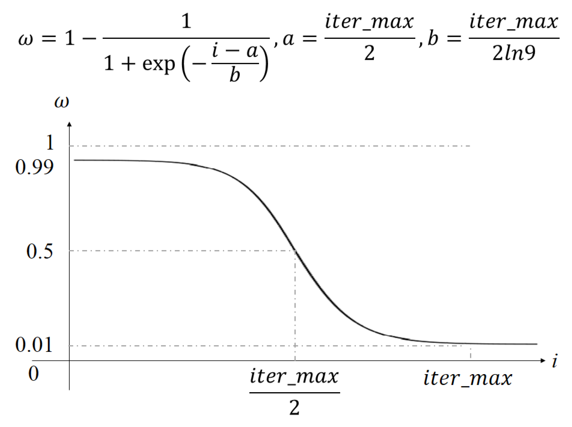
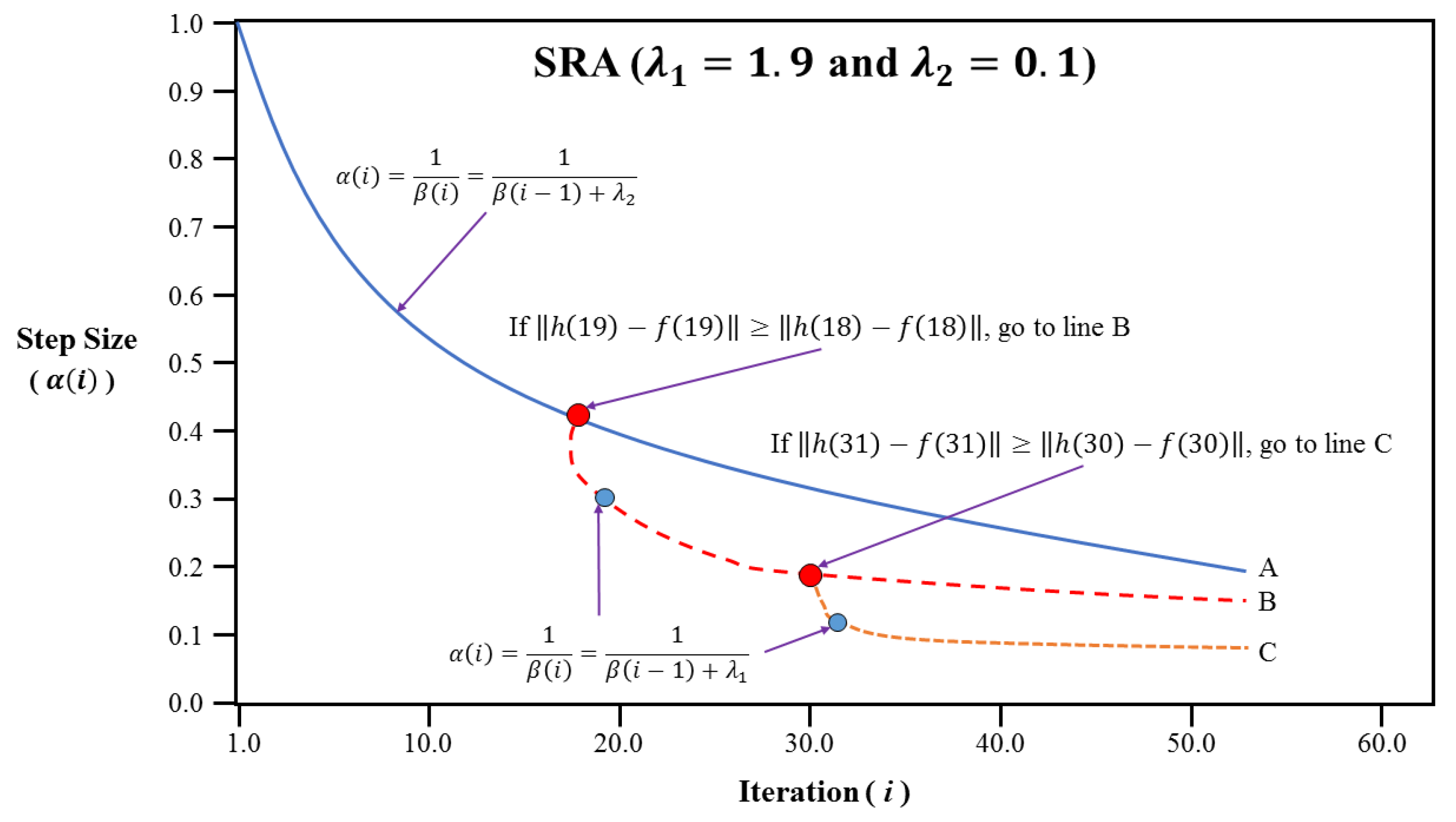
3.3. Improved Algorithms Based on Simulated Annealing Algorithm

Therefore, we summarize some advantages and disadvantages of the Newton method, the ant colony algorithm and the simulated annealing algorithm which are shown as the following Table 4.
From above table, we can see that both ant colony algorithm and the simulated annealing algorithm can solve many problems of the Newton method, and the shortcomings of the ant colony algorithm can also be dealt with the simulated annealing algorithm. Generally speaking, the simulated annealing algorithm has strong global search ability but low solution accuracy. Thus we proposed two improved algorithms based on the simulated annealing algorithm (ISAA-CC and ISAA-SS).
(a) Improved simulated annealing algorithm of cooling coefficient (ISAA-CC).   
The cooling coefficient ω < (0, 1) is an important parameter affecting the convergence of the simulated annealing algorithm from the procedure of this algorithm. When this coefficient is too large, the solution accuracy is high but the algorithm runs long. On the other hand, when this coefficient is too small, the search accuracy is low. Therefore, considering this disadvantages, this paper firstly proposes an improved algorithm based on the simulated annealing algorithm, named ISAA-CC, to improve the efficiency of the algorithm and the quality of the optimal solution.
The value of ω is set as large as possible at the beginning of the algorithm, so that the algorithm has strong global search ability. With the iteration of the algorithm, the value of ω decreases, in order that the algorithm can search for the optimal solution better. As a result, a functional relationship between the cooling coefficient ω and the number of iterations i as shown in Figure 4 will be established as follows.
(b) Improved simulated annealing algorithm of step-size (ISAA-SS).   
Chen et al. [30] used an improved path-based local linearization algorithm to solve a special logit model and used recent advances in line search methods to improve the computational efforts. The experimental results of this article examined two exact line search methods (i.e., bisection and method of successive averages (MSA)) along with three inexact line search methods (i.e., self-regulated averaging (SRA), quadratic interpolation and Armijo). These line search methods are compared in the Table 5 including the computation with respect to the objective function and derivative evaluations.
Numerical results in this paper revealed SRA and quadratic interpolation were more efficient and robust compared to others. The computational efficiency and robustness of them are attributed to their smart step-size determination mechanism. Compared to other methods, SRA is easy to implement because it does not need to evaluate the complex objective function or its derivatives.
The Newton method used in this revised manuscript includes the derivation of the objective function; and the disadvantages of the Newton method compared with the other three heuristic algorithms are its derivatives, as shown in Table 4. Thus we choose embedding SRA to improve the simulated annealing algorithm on determining a suitable step-size, namely ISAA-SS.
In the literature, self-regulated averaging (SRA), was recently developed by Liu et al. [31], to enhance he computational performance of determining a suitable step-size for solving the multinomial logit stochastic user equilibrium (MNL SUE) problem. This method determines a suitable step-size as follows:
α ( i ) = 1 β ( i ) .
β ( i ) = β ( i 1 ) + λ 1 if | | h ( i ) f ( i ) | | | | h ( i 1 ) f ( i 1 ) | | , β ( i 1 ) + λ 2 otherwise ,
where α ( i ) is step-size at iteration i, σ ( i ) is a measure of similarity index and β ( i ) is a measure of dissimilarity index, defined as β ( i ) = 1 σ ( i ) ; and the following conditions should be satisfied in order to guarantee convergence [31,32,33]:
α ( i ) > 0 , i = 1 α ( i ) = and lim i α ( i ) = 0 or i = 1 ( α ( i ) ) 2 < .
An illustration of SRA is provided in Figure 5. From Equation (13), we can observe that the step-size sequences from SRA are still strictly decreasing. However, the decreasing speed is more efficient since the next step-size is determined according to the residual error (i.e., the deviation between the current solution and its auxiliary solution) relationship between two consecutive iterations. When the current residual error is increased compared to the previous iteration (i.e., tends to diverge), the parameter λ 1 > 1 is used to make the step-size reduction more aggressive (e.g., at iterations 19 and 31). In contrast, when the residual error is decreased (i.e., tends to converge), the parameter 0 < λ 2 < 1 is used to make the step-size reduction more conservative. Hence, the step-size sequences from SRA indeed satisfy the above conditions.
In Section 4, we use these five methods, i.e., the Newton method (Appendix A), the ant colony algorithm, the simulated annealing algorithm, two improved algorithms, ISAA-CC and ISAA-SS to solve the problem, and then compare the performance of them. The results show that two improved algorithms proposed in this paper are better than others about solving the optimal solution.

4. Numerical Experiment

Due to the representation of Beijing–Tianjin railway in China which includes all railway traffic modes, it is urgent for us to solve market shares on this line, and to judge the feasibility of operation plan. This real-world case study in Beijing–Tianjin corridor in this section is implemented to verify the applications of the proposed eight utility functions, a mixed logit model and five algorithms. The problems in this paper, i.e., the estimation of unknown parameters, and the solution of likelihood functions are all coded and solved by Python 2.7 Version in Pycharm on Windows 7 personal computer with 3.4 Gb processor.
All data used in this numerical experiment are shown as follows. For example, essential information, including operational frequency, running time and ticket price, of different railway traffic modes in Beijing–Tianjin corridor from 12306.com is shown in Table 6.
According to information of different railway traffic modes above, including running time and ticket price, we can divide all train seats into nine grades which is shown in Table 7.
Then, in this numerical experiment, the Newton method, the ant colony algorithm, the simulated annealing algorithm and two improved algorithms based on the simulated annealing algorithm (ISAA-CC and ISAA-SS) are adopted to solve the model established in this paper, i.e., the mixed logit model based on improved nonlinear utility functions. The likelihood estimator, i.e., θ ^ which is the vector of parameters to be estimated, and the optimal solution, i.e., ϕ ( θ ^ ) of the corresponding objective function are obtained by five algorithms. Among them, the algorithm principle and experimental results of the Newton method are shown in Appendix A.

4.1. Computations of Five Algorithms

4.1.1. Results of Ant Colony Algorithm

There are the results of the ant colony algorithm when initialized parameters are ρ = 0.9, Q = 1, p 0 = 0.2, a n t _ m a x = 110 and i t e r _ m a x = 1000. The choosing probabilities of different passenger groups and market shares of different railway traffic modes are shown in Table 8; and correspondingly the likelihood estimated value is
θ ^ ACA = 0.36649 0.23356 0.14638 0.15491 0.51441 0.16361 0.45006 0.13533 0.17568 0.14163 0.20485 0.39591 0.06941 0.27331 0.06589 0.09424 0.17735 0.45341 0.22754 0.40205 0.34847 0.30527 0.40613 0.40021 0.28048 0.17138 0.42123 0.04713 0.06771 0.25781 0.07792 0.37023 1.32204 1.73792 7.66653 5.99888 0.11048 1.17499 0.61528 3.93062 0.53273 9.00299 7.68427 8.65102 9.76036 3.16137 6.10299 6.54772 .

4.1.2. Computation of Simulated Annealing Algorithm

There are the results of the simulated annealing algorithm when initialized parameters are T 0 = 100, T min = 1 e 3 , ω = 0.9 and i t e r _ m a x = 1000. The choosing probabilities of different passenger groups and market shares of different railway traffic modes are shown in Table 9; and correspondingly the likelihood estimated value is
θ ^ SAA = 0.21408 0.15535 0.29768 0.39595 0.29681 0.03521 0.52151 0.32206 0.19907 0.17063 0.17375 0.39159 0.11105 0.17564 0.08192 0.08671 0.12692 0.35264 0.20979 0.12505 0.26783 0.44408 0.28524 0.44486 0.45993 0.32138 0.31878 0.08741 0.32431 0.34507 0.11133 0.14637 1.70236 6.24121 2.21014 9.34219 0.41057 7.35221 7.17027 5.96812 4.81388 4.11327 4.96551 0.87155 5.61586 3.66091 7.15305 3.22823 .
The models also show that the characteristics of low-income passengers, medium-income passengers and high-income passengers in choosing traffic modes are different, as in Figure 6.
In fact, passenger groups with different income have different consumption habits. Generally speaking, high-income passengers were apt to choose a time-saving, comfort, good service quality and safety secured traffic modes regardless of fare while low-income passengers preferred to economical traffic modes more than high-income passengers; and then medium-income passenger groups often seek a more comfortable travel way with acceptable price, better service quality. The response in above figure is that the choosing probabilities (Orange columns) are basically unchanged.

4.1.3. Computation of ISAA-CC

There are the results of ISAA-CC when initialized parameters are T 0 = 100, T min = 1 e 3 and i t e r _ m a x = 1000. The choosing probabilities of different passenger groups and market shares of different railway traffic modes are shown in Table 10; and correspondingly the likelihood estimated value is
θ ^ ISAA - CC = 0.12386 0.10714 0.08256 0.17758 0.23826 0.13925 0.25367 0.19062 0.21058 0.18295 0.20462 0.49699 0.12364 0.14583 0.09122 0.09442 0.36069 0.37474 0.43201 0.23511 0.17696 0.37751 0.32207 0.38192 0.30487 0.33517 0.28081 0.09032 0.46114 0.33741 0.33304 0.33304 4.44111 1.81442 0.78123 5.81542 3.22075 0.55967 5.87164 6.15154 9.85848 0.88064 2.72219 6.30403 6.88228 0.39592 8.20899 5.41357 .
Then, we test the stability of this improved algorithm proposed in this paper after 30 times experiments, and results including optimum solutions and running time in each calculation are shown in Figure 7.
Moreover, we calculate the mean and variance of these optimum solutions in experiment results to analysis the stability, i.e., E = −1.2721, S 2 = 0.00971 2 = 9.42841 e 05 1 e 03 . So we can conclude that the improved algorithm is very stable. Among them, the maximum optimal solution is −1.25441.

4.1.4. Computation of ISAA-SS

There are the results of ISAA-SS when initialized parameters are T 0 = 100, T min = 1 e 3 and ω = 0.9. The choosing probabilities of different passenger groups and market shares of different railway traffic modes are shown in Table 11; and correspondingly the likelihood estimated value is
θ ^ ISAA - SS = 0.09806 0.08318 0.12239 0.11659 0.17376 0.17589 0.21286 0.22458 0.23704 0.20141 0.22659 0.59322 0.13269 0.16139 0.10224 0.10569 0.33686 0.44118 0.15059 0.03477 0.41618 0.36919 0.31531 0.32482 0.32804 0.27423 0.50043 0.25542 0.27737 0.29353 0.36959 0.34491 2.75383 7.70283 9.17939 8.37879 8.51512 6.56612 4.24546 2.41824 3.11007 7.98969 8.11517 4.14189 7.34061 6.67762 8.42431 0.27669 .

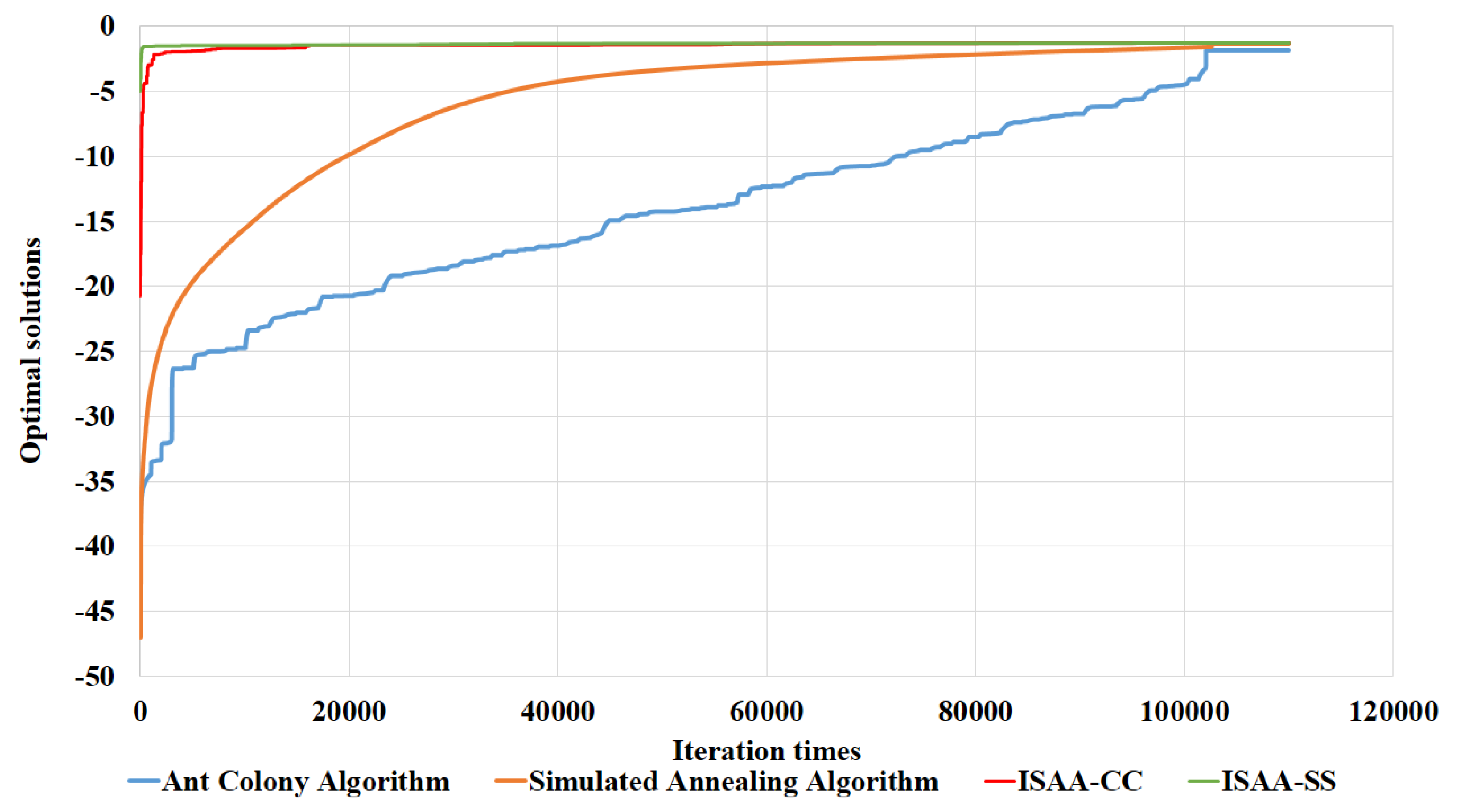
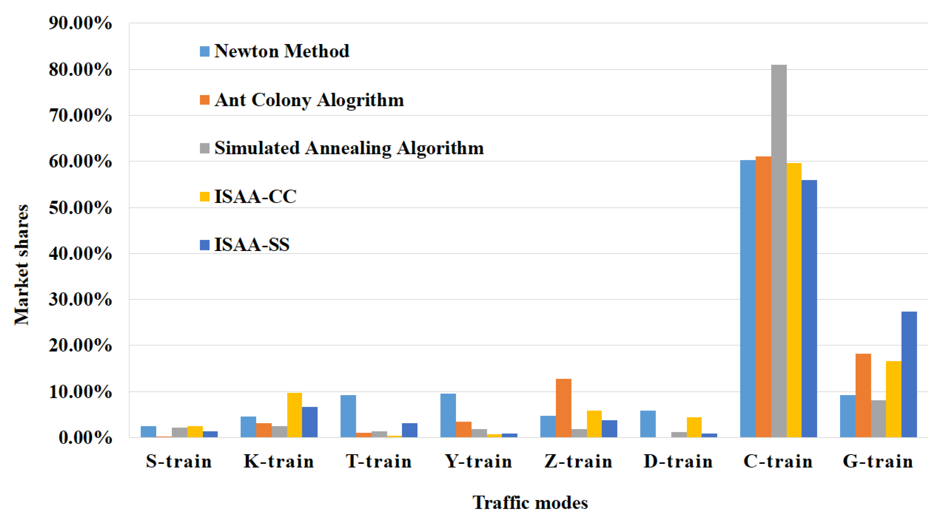
4.2. Contrast of Five Algorithms

There are experimental comparison results of these five algorithms, including the optimum solution of the log-likelihood function and running time, shown in Table 12.
It can be concluded from the above table that ISAA-CC proposed in this paper has the shortest running time and the optimal final objective function value. ISAA-SS proposed in this paper is second to ISAA-CC about the optimum solutions but also is second to the simulated annealing algorithm about the running time.
The functional relationships between the optimum solutions and the iteration times obtained by above four heuristic algorithms are shown in Figure 8. Among them, the horizontal coordinate represents iteration times and vertical coordinates represents the optimal solution of each iteration.
It can be seen from the above figure that, as the times of iterations increases, the simulated annealing algorithm fluctuates greatly during the search process, but after more than 80,000 iterations, the algorithm converges to the optimal solution. Two improved algorithms have faster convergence than the basic one, and they both converge to the optimal solution until about 20,000 iterations. Both are better than the convergence speed of the ant colony algorithm.
In summary, the aim of the model we built is to maximize the log-likelihood function and then in order to maximize utility of all passenger groups. So according to the table and figure above, we can conclude that these two improved algorithm proposed in this paper are the best than any others.
The results, i.e., market shares of different railway traffic modes, calculated by these five algorithms, are shown in Figure 9.
From this figure, we can see that the rankings of market shares solved by all algorithms have no big differences. Subject to ISAA-CC, due to its high speed, appropriate departure time and high running frequency, C-train is one of the most popular railway passenger products in Beijing–Tianjin corridor at any income levels. Not only because of its high speed but also due to its appropriate departure time and high running frequency. On the contrary, both the market shares of S-train and T-train are the smallest in all railway traffic modes due to their slowest speed. Moreover, due to the short travel time from Beijing to Tianjin and the less demand for tourist trains, the market share of Y-train is relatively small. Moreover, we all know that the departure time of D-train is almost at 9 o’clock pm or later and the overnight D-train is mainly established for long-distance passengers, so the market shares of this train is small due to inappropriate departure time.

5. Conclusions and Future Researches

The method of solving market shares proposed in this paper is a common method for managing the passenger flow in order to reduce the mismatch between transportation resources allocation and passenger demand. To characterize the problem in a mathematical way, a mixed logit model based on improved nonlinear utility functions is formulated in this paper. According to maximum likelihood estimation, the likelihood function is formulated to maximize the utility of all passenger groups. Since the proposed model consists of a large number of both variables and parameters, the computational intensity becomes a significant problem in the solution process. In view of this fact, the model is solved by five algorithms, the Newton method, the ant colony algorithm, the simulated annealing algorithm and two improved algorithms based on the simulated annealing algorithm (ISAA-CC and ISAA-SS). Furthermore a real-world instance with operation data of the Beijing–Tianjin corridor is implemented to demonstrate the performance and effectiveness of the proposed approaches. Relatively speaking, the experimental results show that the two improved algorithms proposed in this paper have the shortest running time, the optimal final objective function value and the fastest convergence speed. Furthermore, subject to these two improved algorithms, C-train is one of the most popular railway passenger products in the Beijing–Tianjin corridor. Thus from the enterprise’s point of view, it is recommended that the railway department invest more cost in C-trains to get more passenger demand and operational revenue.
Further research could focus on the following several aspects. (a) With a series of passenger demand data, how to generate a more robust and reliable optimal model is a significant topic for further research. (b) Due to the over-length of this paper, we only designed two improved heuristic algorithms based on the simulated annealing algorithm to solve the problem. More effective heuristic algorithms could also be studied in our future research.

Author Contributions

Conceptualization, B.H.; methodology, B.H.; validation, B.H.; formal analysis, B.H.; investigation, J.B.; resources, B.H. and S.R. and J.B.; data curation, S.R.; writing—original draft preparation, B.H.; writing—review and editing, B.H.; visualization, B.H.; supervision, B.H.; project administration, S.R.; funding acquisition, S.R. and B.H. All authors have read and agreed to the published version of the manuscript.

Funding

This research is funded by National Key R & D Program of China, grant number 2018YFB1201401, and the Fundamental Research Funds for the Central Universities, grant number 2018JBM019.

Conflicts of Interest

(a) Declare conflicts of interest or state: Author Bing Han, Author Shuang Ren and Author Jingjing Bao declare that they have no conflict of interest. (b) Ethical approval: This article does not contain any studies with human participants performed by any of the authors. (c) Informed consent: Informed consent was obtained from all individual participants included in the study.

Appendix A. Newton Method

In this paper, we also estimate the unknown parameters by the Newton method which summarized the procedure in following Algorithm A1.
Algorithm A1: A traditional algorithm.
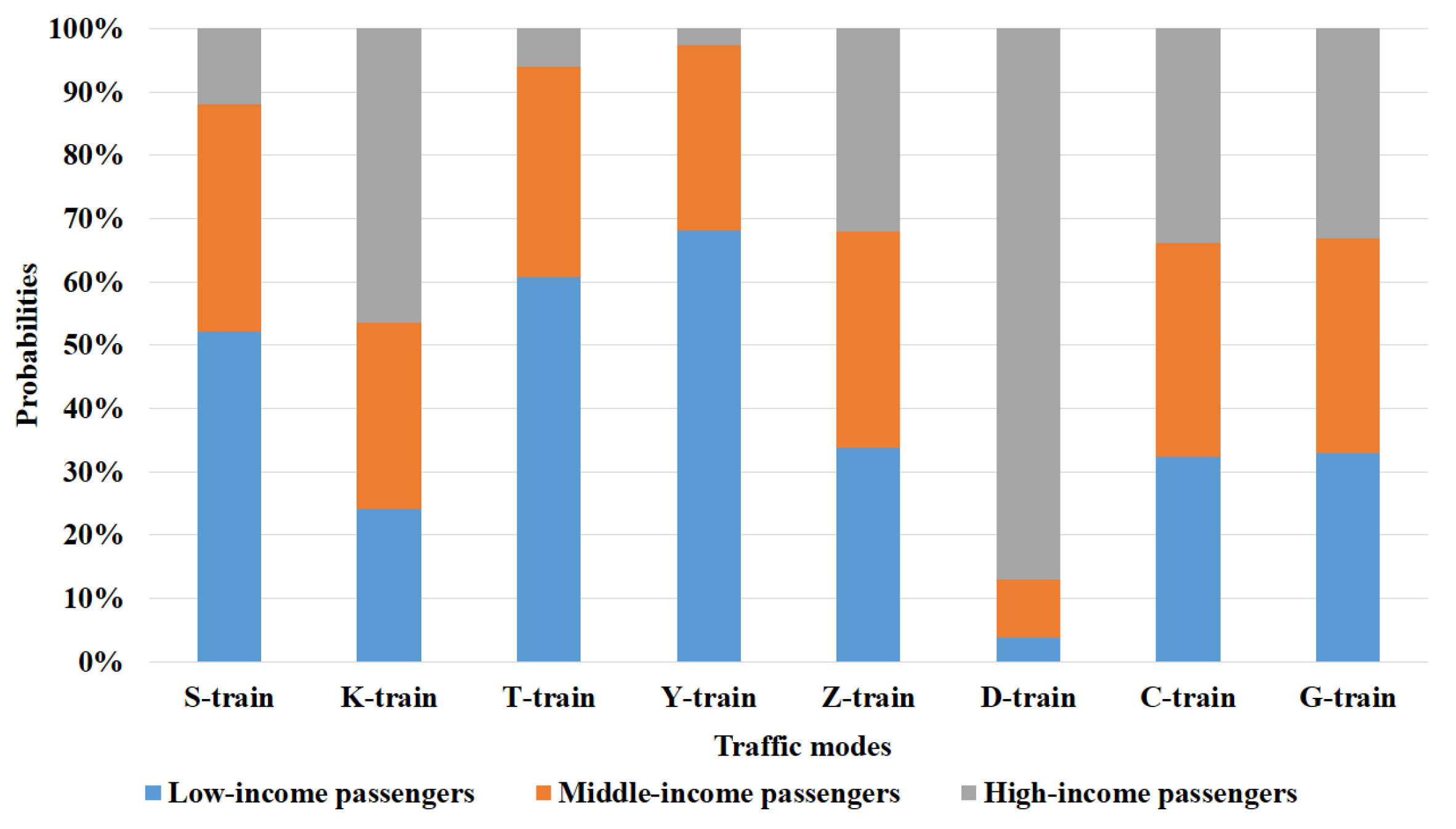
Step 1.
Input the initial value θ ( 0 ) .
Step 2.
If the function ϕ ( θ ) has a continuous second derivative ϕ ( θ ( 0 ) ) of θ ( 0 ) , then the first derivative  ϕ ( θ ( 0 ) ) expands of θ ( 0 ) by ϕ ( θ ) = ϕ ( θ ( 0 ) ) + ϕ ( θ ( 0 ) ) · θ θ ( 0 ) + O θ θ ( 0 ) 2 .
Step 3.
Because of ϕ ( θ ( 0 ) ) =0, put it into that formula, then there is
θ = θ ( 0 ) + ϕ ( θ ( 0 ) ) 1 · ϕ ( θ ( 0 ) ) .
Step 4.
Iterate and return the parameter θ ^ to be estimated according to the iterative formula, i.e., θ ( i + 1 ) = θ ( i ) + ϕ ( θ ( i ) ) 1 · ϕ ( θ ( i ) ) where i is the number of iterations until θ ( i + 1 ) θ ( i ) < ε where ε is sufficiently small.
We can see that the Newton method takes a polynomial solution time because the inverse matrix of the Hessian matrix needs to be solved in each step. There are the results of the Newton method. The parameter values are
θ ^ NM = 0.3768 0.3801 0.3981 0.3033 0.2371 0.1749 0.2441 0.3905 0.3533 0.1105 0.3701 0.2078 0.3312 0.2736 0.3742 0.1987 0.0653 0.2553 0.1692 0.1972 0.3706 0.0871 0.2116 0.3117 0.2046 0.2541 0.0626 0.2917 0.0611 0.4644 0.1701 0.0991 0.7679 8.5023 9.0031 5.4908 5.5263 4.9141 4.8906 5.9355 5.1299 7.6766 5.8837 4.2128 7.0455 9.0535 2.1432 4.1033 .
The probabilities and market shares are shown in Table A1.
Table A1. Market shares computed by the Newton method.
(Unit: %)Probabilities of Different Passenger GroupsMarket Shares
Low-Income PassengersMedium-Income PassengersHigh-Income Passengers
S-train1.955660.519330.012132.48712
K-train3.615390.943790.021084.58026
T-train4.264962.691222.254099.21027
Y-train2.971793.238953.331229.54196
Z-train2.397050.895471.390254.68277
D-train1.494882.839461.566995.90133
C-train25.256018.3576726.7095660.32324
G-train0.629721.292457.252219.17438

References

  1. Train, K.E. Properties of discrete choice models. In Discrete Choice Methods with Simulation; Cambridge University Press: Cambridge, UK, 2003; pp. 15–37. [Google Scholar]
  2. Train, K.E. Properties of discrete choice models. In Discrete Choice Methods with Simulation, Second Edition; Cambridge University Press: Cambridge, UK, 2009; pp. 9–33. [Google Scholar]
  3. Marschak, J. Binary choice constraints on random utility indications. In Economic Information, Decision, and Prediction; Stanford University Press: Stanford, CA, USA, 1960; pp. 312–329. [Google Scholar]
  4. Train, K.E.; McFadden, D.; Ben-Akiva, M. The demand for local telephone service: A fully discrete model of residential calling patterns and service choice. Rand J. Econ. 1987, 18, 109–123. [Google Scholar] [CrossRef]
  5. McFadden, D. Conditional logit analysis of qualitative choice behavior. In Frontiers in Econometrics; Academic Press: New York, NY, USA, 1973; pp. 105–142. [Google Scholar]
  6. McFadden, D. Modelling the choice of residential location. In Cowles Foundation Discussion Papers; Yale University Press: New Haven, CT, USA, 1977; p. 673. [Google Scholar]
  7. Hensher, D.A.; Rose, J.M.; Greene, W.H. Getting started modeling: The workhorse—Multinomial logit. In Applied Choice Analysis; Cambridge University Press: Cambridge, UK, 2015; p. 1188. [Google Scholar]
  8. McFadden, D.; Train, K.E. Mixed MNL models for discrete response. J. Appl. Econom. 2000, 15, 447–470. [Google Scholar] [CrossRef]
  9. Hess, S.; Polak, J.W. Development and Application of a Model for Airport Choice in Multi-Airport Regions; CTS Working Paper; Centre for Transport Studies, Imperial College London: London, UK, 2004. [Google Scholar]
  10. Hensher, D.; Greene, W.H. The mixed logit model: the state of practice. Transportation 2003, 30, 133–176. [Google Scholar] [CrossRef]
  11. Hess, S.; Polak, J.W. On the use of discrete choice models for airport competition with applications to the San Francisco Bay area Airports. Paper presented at the 10th Triennial World Conference on Transport Research, Istanbul, Turkey, 4–8 July 2004. [Google Scholar]
  12. Hess, S.; Polak, J.W. Mixed logit estimation of parking type choice. In Proceedings of the 83rd Annual Meeting of the Transportation Research Board, Washington, DC, USA, 11–15 January 2004. [Google Scholar]
  13. Ma, B.T.; Zhang, Y.X.; Zhao, C.X. Estimation of the distributing rates of high-speed passenger flows with the logit model. J. North. Jiaotong Univ. 2003, 27, 67–69. [Google Scholar]
  14. Hess, S.; Polak, J.W. Mixed logit modeling of airport choice in multi-airport regions. J. Air Transp. Manag. 2005, 11, 59–68. [Google Scholar] [CrossRef] [Green Version]
  15. He, Y.Q.; Mao, B.H.; Chen, T.S.; Yang, J. The mode share model of the high-speed passenger railway line and its application. J. China Railw. Soc. 2006, 28, 18–21. [Google Scholar]
  16. Park, Y.; Ha, H.K. Analysis of the impact of high-speed railroad service on air transport demand. Transp. Res. Part E Logist. Transp. Rev. 2006, 42, 95–105. [Google Scholar] [CrossRef]
  17. Feng, H.H.; Zhu, C.K. Application of rough set theory in the Inter-city passenger traffic sharing. J. Univ. Sci. Technol. Suzhou Eng. Technol. 2007, 20, 30–33, 38. [Google Scholar]
  18. Ge, D.S.; Liu, Z.K. Research on mixed logit model improved by value engineering method. Value Eng. 2008, 1, 78–80. [Google Scholar]
  19. Jou, R.C.; Hensher, D.A.; Hsu, T.L. Airport ground access mode choice behavior after the introduction of a new mode: A case study of Taoyuan International Airport in Taiwan. Transp. Res. Part E Logist. Transp. Rev. 2011, 47, 371–381. [Google Scholar] [CrossRef]
  20. Huang, D.M.; Qin, S.H.; Zhao, C.C. Application of logit model in passenger flow sharing forecast of Nan-Guang high-speed railway. Railw. Eng. 2012, 11, 45–48. [Google Scholar]
  21. Chen, J.; Yan, Q.P.; Yang, F.; Hu, J. SEM-logit integration model of travel mode choice behaviors. J. South China Univ. Technol. Nat. Sci. Ed. 2013, 41, 51–57, 65. [Google Scholar]
  22. Hensher, D.; Greene, W.H. Passenger airline choice behavior for domestic short haul travel in South Korea. J. Air Transp. Manag. 2014, 38, 43–47. [Google Scholar]
  23. Lee, J.K.; Yoo, K.E.; Son, K.H. A study on travelers’ railway traffic mode choice behavior using the mixed logit model: A case study of the Seoul-Jeju route. J. Air Transp. Manag. 2016, 56, 131–137. [Google Scholar] [CrossRef]
  24. Fishburn, P.C. Utility Theory. Manag. Sci. 1968, 14, 335–378. [Google Scholar] [CrossRef] [Green Version]
  25. Wardman, M. The value of travel time a review of British evidence. J. Transp. Econ. Policy 1998, 32, 285–316. [Google Scholar]
  26. Dorigo, M. Optimization, Learning and Natural Algorithms. Ph.D. Thesis, Politecnico di Milano, Milan, Italy, 1992. [Google Scholar]
  27. Dorigo, M.; Member, S.; Gambardella, L.M. Ant colony system: A cooperative learning approach to the traveling salesman problem. IEEE Trans. Evol. Comput. 1996, 1, 53–66. [Google Scholar] [CrossRef] [Green Version]
  28. Metropolis, N. Algorithms in unnormalized arithmetic. Numer. Math. 1953, 7, 104–112. [Google Scholar] [CrossRef]
  29. Kirkpatrick, S.; Gelatt, C.D.; Vecchi, M.P. Ant Colony System: A cooperative learning approach to the traveling salesman problem. Science 1983, 220, 671–680. [Google Scholar] [CrossRef]
  30. Chen, A.; Ryu, S.; Xu, X.D.; Choi, K. Computation and application of the paired combinatorial logit stochastic user equilibrium problem. Comput. Oper. Res. 2014, 43, 68–77. [Google Scholar] [CrossRef]
  31. Liu, H.; He, X.; He, B.S. Method of successive weighted averages (MSWA) and self-regulated averaging schemes for solving stochastic user equilibrium problem. Netw. Spat. Econ. 2009, 9, 485–503. [Google Scholar] [CrossRef]
  32. Robbins, H.; Monro, S. A stochastic approximation method. Ann. Math. Stat. 1951, 22, 400–407. [Google Scholar] [CrossRef]
  33. Blum, J.R. Multidimensional stochastic approximation methods. Ann. Math. Stat. 1954, 25, 737–744. [Google Scholar] [CrossRef]
Figure 1. The technical route.
Sustainability 12 01406 g001
Figure 2. Curves of travel time, travel expense and comfort degree.
Sustainability 12 01406 g002
Figure 3. Passenger income function.
Sustainability 12 01406 g003
Figure 4. Relationship between cooling coefficient and the number of iterations.
Sustainability 12 01406 g004
Figure 5. Illustration of self-regulated averaging (SRA).
Sustainability 12 01406 g005
Figure 6. Characteristics of different income passengers in choosing traffic modes.
Sustainability 12 01406 g006
Figure 7. Final solutions of 30 times experiments.
Sustainability 12 01406 g007
Figure 8. Iterative process comparison of three heuristic algorithms.
Sustainability 12 01406 g008
Figure 9. Comparison of five algorithms in solving market shares.
Sustainability 12 01406 g009
Table 1. Recent publications on logit models in comparison with our work.
PublicationTraffic modesVariablesModels
Ma, et al. [13]Airport, Coach, RailwaySafety, rapidity, economy, comfort, environmental impact, servicesConditional logit model
Hess, et al. [14]AirportAccess time, fare, frequencyMixed logit model
He, et al. [15]Airport, Coach, High Speed Passenger dedicated lineFare, time valueConditional logit model
Park, et al. [16]Airport, High Speed Railway (KTX), Conventional railroadAccess time, fare, operational frequency, distanceBinomial logit model and SP/RP model
Feng, et al. [17]Airport, Coach, TrainFare, time valueLogit model based on Rough Set Theory
Ge, et al. [18]Airport, Coach, RailwaySafety, rapidity, economy, choice preference, comfort, accessibilityMixed logit model
Jou, et al. [19]High Speed Railway, Hyper-speed TransportationIn-vehicle travel time, travel cost, out-of-vehicle travel timeMixed logit model
Huang, et al. [20]Airport, Coach, High Speed RailwayFare, time valueMultinomial logit model
Chen, et al. [21]BusService environment, comfort, safety, convenienceSEM-Multinomial logit integration model
Jung, et al. [22]Korea Train ExpressAccess time, journey time, air fare, operational frequencyMultinomial and nested logit model
Lee, et al. [23]High Speed RailwayTravel cost, travel time, operational frequency, safety, duty free shopping availabilityMixed logit model
This paperDifferent railway traffic modesPassenger income, rapidity (travel time), Economy (travel expense), comfort (operational frequency, degree of seat)Mixed logit model based on improved nonlinear utility functions
Table 2. The travel consideration factors for different passenger groups (unit: People).
Passenger GroupsRapidityEconomyComfortTotal Number
Low-income passengers762912117
Medium-income passengers2145573342
High-income passengers1632768258
Total number453111153717
Table 3. Parameters and variables in the model.
Model Parameters
MA set of railway traffic modes, i.e., M = {1, 2, ⋯, 8}. There are eight (M = 8) kinds of railway trains for passengers to choose in this study, including Common slow train named S-train, i.e., m = 1, Fast train named K-train, i.e., m = 2, Express train named T-train, i.e., m = 3, Tourist train named Y-train, i.e., m = 4, Direct special express train named Z-train, i.e., m = 5, EMU train named D-train, i.e., m = 6, Inter-city train named C-train, i.e., m = 7 and High-speed train named G-train, i.e., m = 8.
SA set of train seats grades, i.e., S = {1, 2, ⋯, 9}. There are twenty-one kinds of train seats for passengers to choose in this study which are classified into nine grades (S = 9), including business seat of C-train \ G-train, i.e., s = 1, Soft sleeper of D-train, i.e., s = 2, Hard sleeper of D-train, i.e., s = 3, Soft sleeper of S-train \ K-train \ T-train \ Z-train, i.e., s = 4, First seat of C-train \ G-train, i.e., s = 5, First seat of S-train \ K-train \ T-train, i.e., s = 6, Second seat of C-train \ G-train \ D-train, i.e., s = 7, Soft seat of Y-train, i.e., s = 8 and Hard seat of S-train \ K-train \ T-train \ Y-train, i.e., s = 9.
QA set of passenger groups, i.e., Q = {1, 2, 3}. There are three passenger groups, including the low-income passenger group where q = 1, the medium-income passenger group where q = 2 and the high-income passenger group where q = 3.
t m The travel time of passengers choosing railway traffic mode m.
e m The travel expense of passengers choosing railway traffic mode m.
s q The monthly average income of passenger group q.
T max A parameter of maximum time required to fatigue recovery which equals to 14 or 15 hours under normal conditions.
β m s Dimensionless parameter of seat degree s for passengers choosing railway traffic mode m.
γ m s The intensity factor of fatigue recovery time in per unit travel time (Unit: hour 1 ). The greater its value is, the longer fatigue recovery time will be; and there is 0 < γ m s < 1.
Model Variables
θ m The variable vector to be estimated of choosing railway traffic modes m, i.e., θ m = ( α m 1 , α m 2 , α m 3 , α m 4 , μ m , σ m ) T , m M , where α m 1 denotes the weight of rapidity, α m 2 denotes the weight of economy, α m 3 denotes the weight of comfort, α m 4 denotes the weight of passenger income, μ m denotes a position parameter and σ m denotes a scale parameter. There are α m 1 + α m 2 + α m 3 + α m 4 = 1, 0 < α m 1 < 1, 0 < α m 2 < 1, 0 < α m 3 < 1, 0 < α m 4 < 1.
Table 4. The comparisons of three traditional algorithms.
AlgorithmAdvantagesDisadvantages
Newton methodThe simple principle
Second order convergence
(a) It is quite computationally expensive because it requires calculating both the objective function and derivatives. (b) It is highly correlated with initial parameters because the improper selections of them will lead to local convergence or non-convergence of function. (c) Gradient explosion or gradient disappearance also occurs easily.
Ant colony algorithmparallel computation
Robustness
Positive feedback mechanism
Low time complexity
The setting of parameters has a great influence on the results. In the initial stage, the pheromones are basically the same, which requires a long search time and is easily trapped in local optimum.
Simulated annealing algorithmparallel computation
Low time complexity
Independent of the initial solution
It is easy to be affected by the setting of parameters, especially the cooling coefficient.
Table 5. Comparisons of the line search methods.
Line Search MethodsTypeObjective Function EvaluationDerivative Evaluation
MSAexactNoNo
SRAinexactNoNo
BisectionexactNoYes
Quadratic interpolationinexactNoYes
ArmijoinexactYesYes
Table 6. Information of different railway traffic modes.
TypeTraffic ModesFrequencyRunning TimeTicket Price
S-trainCommon slow train32 h 10 minSoft sleeperHard sleeperHard seat
RMB 99.5RMB 64.5RMB 18.5
K-trainFast train132 hSoft sleeperHard sleeperHard seat
RMB 102.5RMB 67.5RMB 21.5
T-trainExpress train51 h 40 minSoft sleeperHard sleeperHard seat
RMB 99.5RMB 65.5RMB 19.5
Y-trainTourist train11 h 30 minSoft seatHard seat-
RMB 33.5RMB 21.5-
Z-trainDirect special61 h 20 minSoft sleeper--
express train RMB 102.5--
D-trainEMU train31 h 10 minSecond seatSoft sleeperHard sleeper
RMB 24RMB 141RMB 102
C-trainInter-city train10030 minBusiness seatFirst seatSecond seat
RMB 174RMB 88RMB 54.5
G-trainHigh-speed train5330 minBusiness seatFirst seatSecond seat
RMB 174.5RMB 94.5RMB 54.5
Table 7. Information of different seat grades.
Seat GradesGrades β ms T min γ ms
Business seat of C-train and G-trainFirst990.150.1
Soft sleeper of D-trainSecond890.170.2
Hard sleeper of D-trainThird790.190.3
Soft sleeper of Z-train, T-train, K-train and S-trainFourth690.210.4
First seat of C-train and G-trainFifth590.250.5
Hard sleeper of T-train, K-train and S-trainSixth490.30.6
Second seat of C-train, G-train and D-trainSeventh390.380.7
Soft seat of Y-trainEight290.50.8
Hard seat of Y-train, T-train, K-train and S-trainNinth190.750.9
Table 8. Market shares computed by the ant colony algorithm.
(Unit: %)Probabilities of Different Passenger GroupsMarket Shares
Low-Income PassengersMedium-Income PassengersHigh-Income Passengers
S-train0.194930.043190.000310.23843
K-train1.796521.158370.143463.09835
T-train0.093470.209110.726721.02929
Y-train0.504150.947392.063733.51527
Z-train9.215363.456050.1001412.77155
D-train0.000840.001940.007610.01039
C-train20.3158824.4842916.2391261.03929
G-train1.213023.0245414.0598718.29743
Table 9. Market shares computed by the simulated annealing algorithm.
(Unit: %)Probabilities of Different Passenger GroupsMarket Shares
Low-Income PassengersMedium-Income PassengersHigh-Income Passengers
S-train1.122590.774710.256782.15408
K-train0.617820.761541.194992.57435
T-train0.819840.449440.080371.34965
Y-train1.236490.528620.048541.81365
Z-train0.617270.626850.585221.82934
D-train0.048230.116321.104441.26899
C-train26.2126827.3324627.3892180.93435
G-train2.658412.743412.673778.07559
Table 10. Market shares computed by ISAA-CC.
(Unit: %)Probabilities of Different Passenger GroupsMarket Shares
Low-Income PassengersMedium-Income PassengersHigh-Income Passengers
S-train0.653060.532410.306141.49161
K-train2.223912.155811.971756.35147
T-train0.894050.973121.214113.08128
Y-train0.292160.262480.195840.75048
Z-train0.806450.752320.620842.17961
D-train0.614480.611190.598921.82459
C-train17.7836618.0398918.6351254.45867
G-train10.0655610.006099.7906429.86229
Table 11. Market shares computed by ISAA-SS.
(Unit: %)Probabilities of Different Passenger GroupsMarket Shares
Low-Income PassengersMedium-Income PassengersHigh-Income Passengers
S-train0.474260.458930.411961.34515
K-train2.281112.237592.083126.60182
T-train0.793750.935981.427193.15692
Y-train0.095460.158450.604170.85808
Z-train1.137721.220991.446413.80512
D-train0.435910.324850.144780.90554
C-train18.3957518.6465818.9544555.99678
G-train9.719399.349958.2612527.33059
Table 12. Comparison results of five algorithms in this numerical experiment.
NMACASAAISAA-CCISAA-SS
Optimum solutions−2.39049−1.82703−1.29297−1.25441−1.25924
Running time60,904 s1927 s518 s205 s858 s

