Determination of the Peak Hour Ridership of Metro Stations in Xi’an, China Using Geographically-Weighted Regression

Department of Traffic Engineering, College of Transportation Engineering, Chang’an University, Xi’an 710064, China
*
Author to whom correspondence should be addressed.
Sustainability 2020, 12(6), 2255; https://0-doi-org.brum.beds.ac.uk/10.3390/su12062255
Submission received: 4 February 2020
/
Revised: 10 March 2020
/
Accepted: 11 March 2020
/
Published: 13 March 2020
(This article belongs to the Collection Sustainable Rail and Metro Systems)
Abstract
:The ridership of a metro station during a city’s peak hour is not always the same as that during the station’s own peak hour. To investigate this inconsistency, this study introduces the peak deviation coefficient to describe this phenomenon. Data from 88 metro stations in Xi’an, China, are used to analyze the peak deviation coefficient based on the geographically weighted regression model. The results demonstrate that when the land around a metro station is mainly land for work, primary and middle schools, and residences, its station’s peak hour is consistent with the city’s peak hour. Additionally, the station’s peak hour is more likely to deviate from the city’s peak hour for suburban stations. There are two ridership options when designing stations, namely the extra peak hour ridership during a city’s peak hour and that during a station’s peak hour, and the larger of the two is used to design metro stations. The mixed land use ratio must be considered in urban land use planning, because although non-commuting land can mitigate the traffic pressure of a city’s peak hour, it may cause the deviation of the station’s peak hours from that of the city.
1. Introduction
According to the Transit Capacity and Quality of Service Manual, the calculation procedure for a desired station’s platform size includes choosing the corresponding average number of passengers, adjusting for passenger characteristics as appropriate, estimating the maximum passenger demand for the platform at a given time, and calculating the required waiting space by multiplying the average space per person by the maximum passenger demand [1]. Estimating the maximum passenger demand for a platform at a given time is one of the most important steps for station design. In China, the Code for Design of Metro (the most recent edition of which is from 2003) states that the capacity of a metro station must be determined by the extra peak hour passenger flow, which is the predicted peak hour passenger flow multiplied by the extra peak hour factor, which is between 1.1 and 1.4 [2]. The predicted result for a metro station is extracted from the predicted result of the metro network, as the total passenger flow volume of the metro network must be controlled to reduce forecasting errors [3]. Today, macroscopic passenger flow forecasting still uses the four-step model [4], which was primarily developed for the prediction of traffic on a regional scale [5] and the evaluation of large-scale infrastructure projects [6]. Thus, the predicted ridership of a station is always in the city’s peak hour, and it determines the station design [7]. However, surveys of urban rail transit operations have shown that, in many areas, a station’s peak hours are not always the same as the city’s peak hours [8]. When designing stations, designers are clearly biased toward adopting station ridership during the city’s (and not the station’s) peak hours. This will increase the difficulty of both passenger flow forecasting in the planning stage and train departure intervals and station management in the operation stage. Because there is only one train departure interval in a period of time in a section of a metro line, if a station’s peak hour is different from those of other stations, the train departure interval will be greater in this station‘s peak hour, and passengers will pile up.
The latest edition of the Code for Prediction of Urban Rail Transit Ridership in China (2016) states that, for the stations in which the passenger flow peak does not appear within the morning and evening peak hours of the city, the station’s own peak hour and passenger flow volume should be predicted [9]. Due to the lack of a theoretical basis, rail transit passenger flow forecast reports for each city can only provide results from a qualitative angle. Therefore, the enlargement coefficient of the passenger flow volume during the peak hours of a station should be determined. This means that, in future rail transit station design, the predicted passenger flow volume during a city’s peak hours can be multiplied by the expanded multiple, thereby providing a more accurate foundation for station design.
The goal of this study is to determine an easy way to convert the ridership in a city’s peak hour as predicted by the four-step method to the ridership in the station’s peak hour while simultaneously retaining the advantages of the four-step method in the control of the total volume of the entire metro network. With regard to the extra peak hour factor, this paper introduces the peak deviation coefficient (PDC), which is the ratio between the predicted ridership of a metro station during its peak hour and the predicted ridership of this metro station during the city’s peak hour. After forecasting the future ridership during the city’s peak hour, the ridership in the station’s peak hour can be calculated from the predicted results via multiplication by the PDC. When designing a new metro line, the land use planning along the metro line will also be conducted simultaneously. Thus, by the analogy of the relationship between the land use around the existing station and the PDC, the considered value of the PDC in the planned station can be determined. The aim of this paper is to analyze the relationship between the influencing factors and the PDC. Because urban development is not at equilibrium and the geographically weighted regression (GWR) model can reflect the spatial heterogeneity, the spatial characteristics of the PDC and its influencing factors are investigated based on the GWR model.
2. Literature Review
With the development of urban rail transit, the research on passenger flow forecasting has continuously deepened and has yielded many results. Scholars first studied the four-step model, which is a family of interrelated models (generation, distribution, assignment, and mode choice), and gradually formed a more mature passenger flow forecasting method [10,11,12,13]. Researchers then began to consider the total control and distribution of passenger flow in the rail transit network [3]. With the construction and operation of urban rail transit, some scholars began to analyze the shortcomings of the traditional four-step model [14,15] and carry out improvement measures [16].
The four-step method is one of the best tools for predicting travel volume [17]. However, it is more suitable for large-scale traffic predictions rather than station-level forecasting. It cannot be used to determine a station’s peak hour, as a station is small compared to the entire metro network. Many scholars have therefore attempted to analyze the characteristics and influences of time-varying passenger flow. Feng et al. [18] analyzed a proportional distribution of the hourly station ridership to the daily station ridership, and others have found that land use [19] or the surrounding environment [20,21], employment, and population [22] influence the diurnal pattern of station passenger flow. Sung and Oh [23] developed different multiple regression models for the day and week. He et al. [24] used a metro ridership estimation method to investigate station-level metro ridership at different times (day of the week, week of the month, and month of the year). Although these studies were not aimed at the investigation of the influence of the degree of the peak hour deviation of station passenger flow, this type of research is a component of the time distributions of metro stations. Therefore, these studies can provide references for the research of the present study.
Other scholars have used Bayesian networks [25], multivariate regression [26], bi-directional long short-term memory networks [27], time series and regression models [28], and back propagation neural networks [29] to predict short-term passenger flow during a station’s peak hour. However, these methods are not suitable for stations that have not yet been constructed.
Few studies have been conducted on passenger flow during a station’s peak hour. Shen [30] proposed the concept of two types of station ridership during peak hours, namely the ridership during the city’s peak hour and the ridership during the station’s peak hour; however, the study provided no research data. Others have found that a station’s peak hour is related to the station’s land use [31,32], location, and travel purposes [8].
Fotheringham [33] proposed the geographically weighted regression (GWR) model, which accounts for spatial heterogeneity. The GWR model is suited to solve the problems related to spatial autocorrelation and non-stationarity in traffic system modeling [34] and has been used to analyze traffic accidents [35], car ownership [36], average annual road traffic [37], public transport use [38], and the relationship between transport and land use [39]. The GWR model has also been used to account for spatial autocorrelation and non-stationarity at the station level [5,21,40].
Because urban development is not at equilibrium, the present research on the peak hour of metro stations was carried out on the basis of previous studies of stations’ peak ridership during this time. Thus, this paper puts forward an enlargement coefficient called peak deviation coefficient (PDC), which can be used to convert the ridership during a city’s peak hour to that during a station’s peak hour. Considering the uneven development around the city center in most cities and the character of the GWR model, the GWR is used in the present study to analyze the relationship between influencing factors and the peak deviation coefficient.
3. Data Sources and Variables
3.1. Data Sources
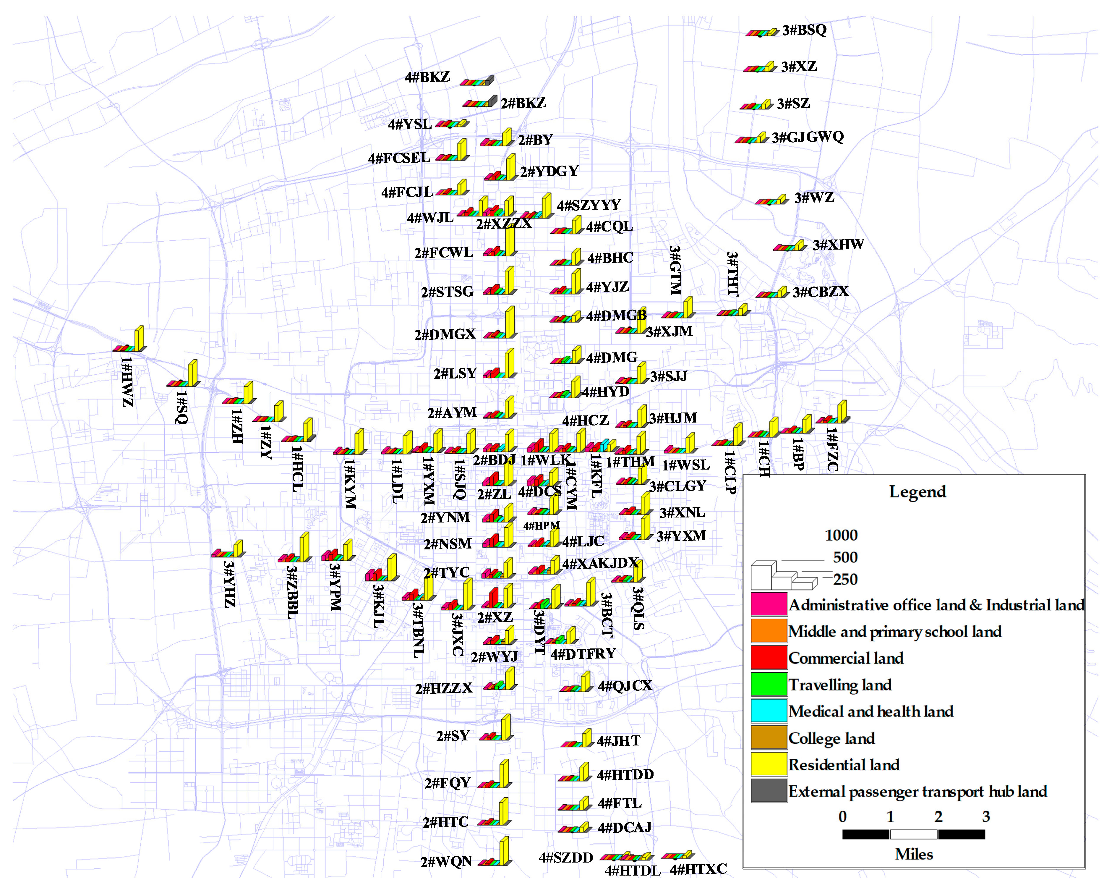
The object of this study is the 88 metro stations in Xi’an, China. It should be noted that the station names consist of two parts. The first component is the number of the line that the station belongs to, so for example, 1# represents Line 1, and the number of the transfer station is the line that was operated earlier. The second part is the initials of the station name. The data includes: 1) The location of metro stations in Xi’an and whether the station is a transfer station or not, according to information collected by the Baidu coordinate pickup system in 2018; 2) The automatic fare collection system (AFC) credit card data of the Xi’an metro in March 2019, provided by Xi’an Metro Co., Ltd.; 3) Land use and building density around stations, which were collected using Baidu Maps. The land use of Xi’an metro stations is shown in Figure 1.
3.2. Dependent Variable
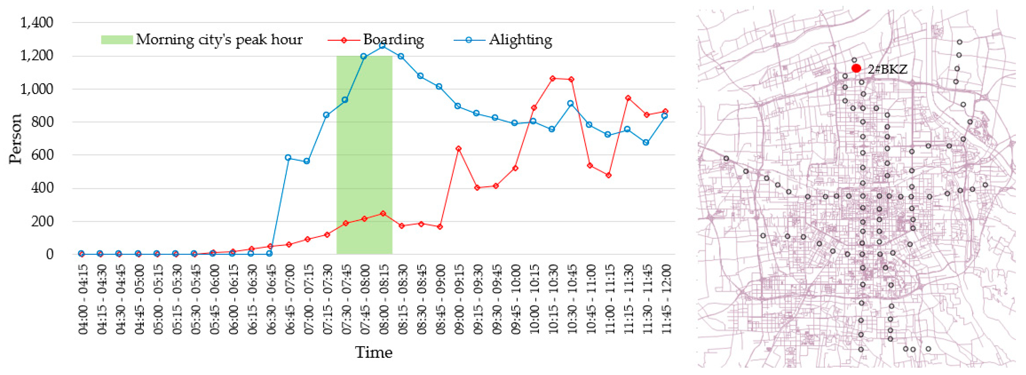
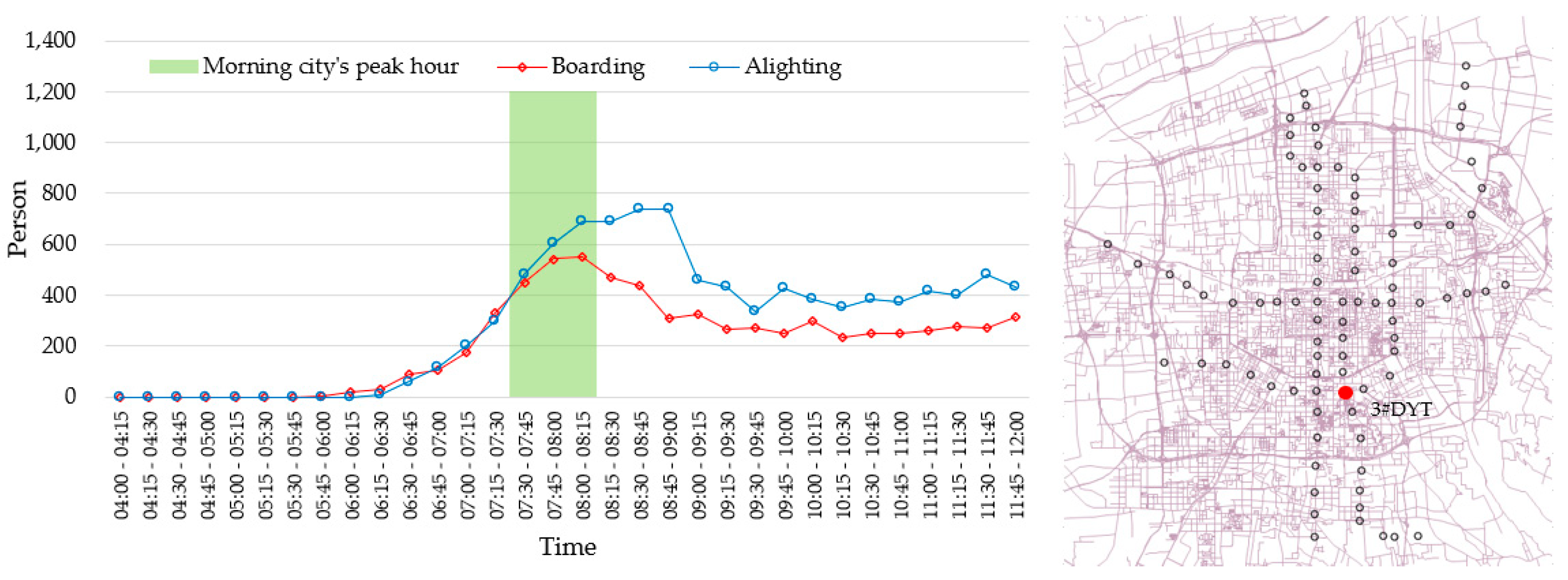
A station’s peak hour refers to the single hour of the day with the highest hourly ridership of the urban rail transit station, whereas a city’s peak hour refers to the single hour of the day that has the highest number of trips throughout the city. For example, the time distributions in the morning of three metro stations are presented in Figure 2, Figure 3 and Figure 4. 1#CLP is in the urban area of Xi’an, 2#BKZ is co-built with a high-speed rail station, and 3#DYT is near a popular tourist spot, the Greater Wild Goose Pagoda Square. The boarding or alighting peak hours of these stations are incongruent with the city’s peak morning hour.
The predicted ridership of metro stations during a city’s peak hour is provided in the forecasting of passenger flow. The peak deviation coefficient (PDC) is used in this study to facilitate the conversion of ridership during a city’s peak hour to that during a station’s peak hour; the coefficient is the ratio between the predicted ridership of a metro station during its own peak hour and the predicted ridership of this metro station during the city’s peak hour. The calculation formula of the PDC is as follows:
where Ps is the ridership of a metro station during its own peak hour and Pc is the ridership of this metro station during the city’s peak hour, and PDC is the peak deviation coefficient. The closer the value of the PDC is to 1, the more similar the ridership at the station’s peak hour is to the ridership at the city’s peak hour.
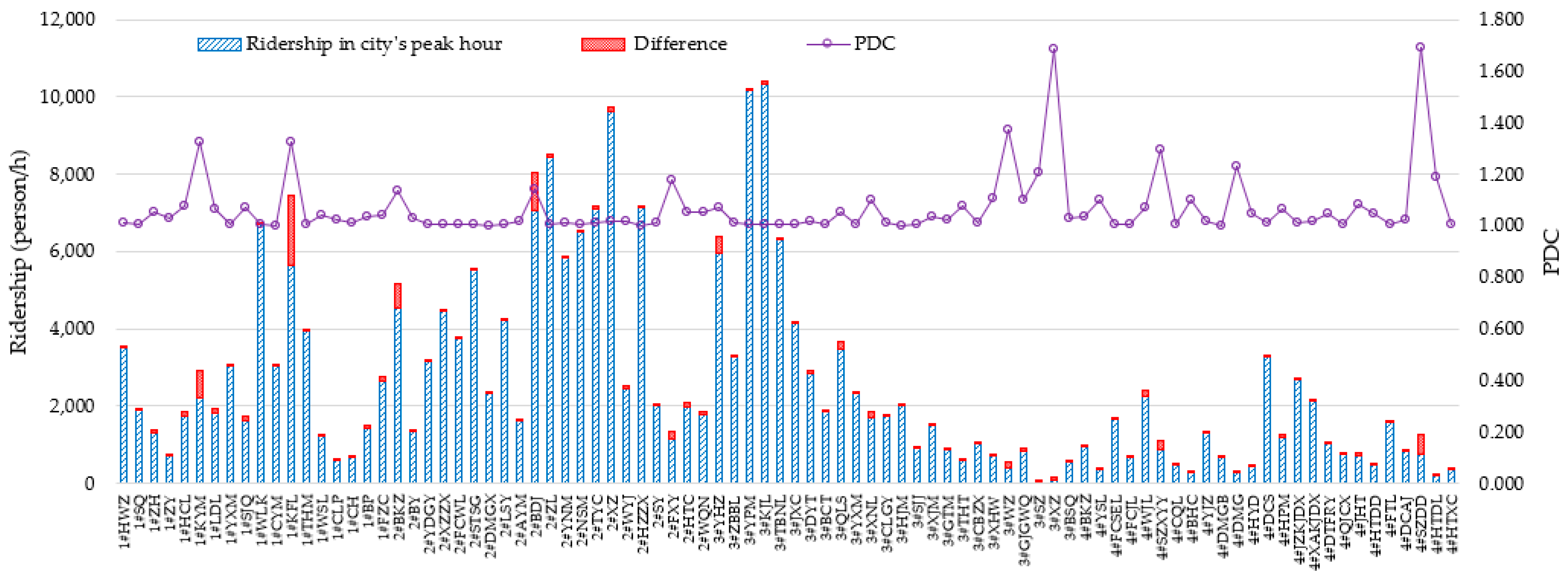
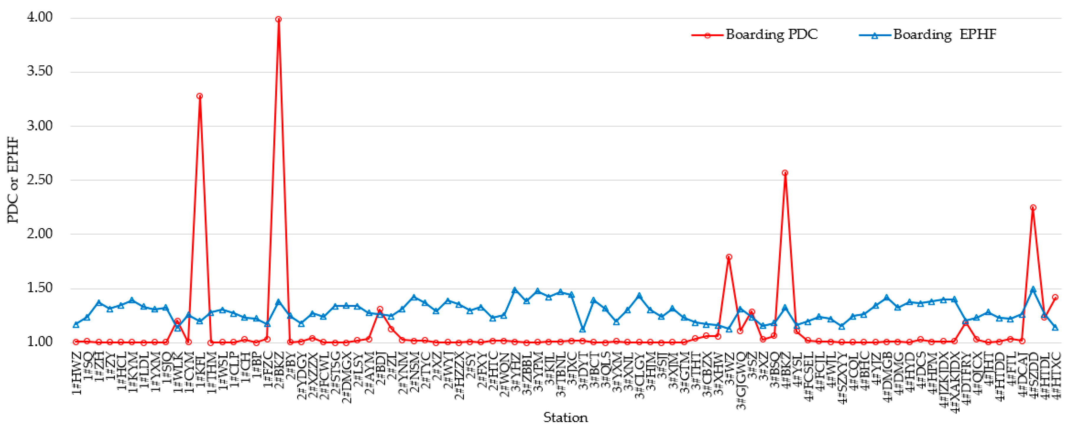
In this study, the boarding and alighting PDC values in the morning were calculated separately. PDCb denotes the boarding PDC, and PDCa denotes the alighting PDC; both are dependent variables. The boarding and alighting ridership in a city’s peak hour, the difference between ridership during a station’s peak hour and the city’s peak hour, and the PDC values of Xi’an metro stations in the morning are presented in Figure 5 and Figure 6. Most PDC values are near 1, indicating that these stations’ peak hours align with the city’s peak hour. However, there are also some stations with a PDC value greater than 1, and some with a PDC value even greater than 1.4. Table 1 presents the morning and evening PDC values of 52 stations of Chongqing metro lines 1, 3, and 6 [41]. It can be seen that although most PDC values are in the range of 1–1.2, 7.69% and 13.46% of stations’ morning and evening PDCs, respectively, are found to be greater than 1.2. Thus, the phenomenon of the ridership of a metro station during a city’s peak hour not always being the same as that during a station’s own peak hour is not a unique case in Xi’an. For the sake of the meticulous design and sustainable development of metro systems, it is important to study the PDC.
It can be determined from Figure 5 and Figure 6 that, when the PDC is large, there may be two conditions. The first condition is that the difference between the ridership during a station’s peak hour and the city’s peak hour is very large compared to that of other stations, such as is the case for 1#KFL and 2#BKZ. The second condition is that the difference between the ridership during a station’s peak hour and the city’s peak hour is small compared to that of other stations, but the station ridership itself is small, and as a result the PDC becomes large, such as is the case for 3#WZ and 4#SZDD.
3.3. Independent Variable Selection
Research on the peak hours of metro stations is still in the initial stage, and is classified as the forecasting of the temporal distribution of station ridership. Therefore, this paper uses the direct station ridership model as a reference, and determines the influence factors of the PDC. The direct station ridership model generally categorizes the influence factors of station ridership into four classes: the built environment, population, social economy, and station characteristics [42].
3.3.1. Built Environment
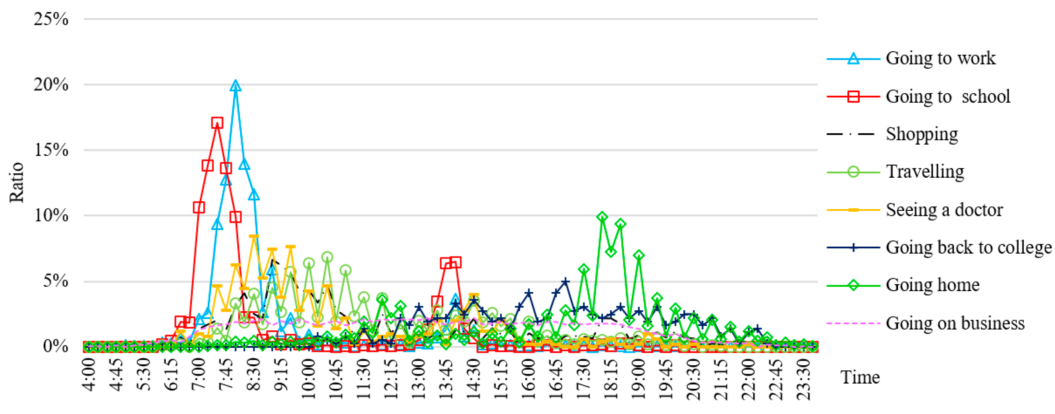
The peak hours of trips are always different. People’s trips can be classified into two kinds according to the consistency of the city’s peak hour. The peak hour of the first kind of trip is consistent with the city’s peak hours, such as going to work and going to school. The peak hour of the second kind of trip is not consistent with the city’s peak hours, such as traveling for shopping. Because different land uses attract different purposes of trips, the ratio of land use ultimately determines the peak hour of the station. Thus, the proportion of the commuting area has an impact on the PDC.
The proportion of the commuting area refers to the proportion of land area that can generate commuter travel to the total land area. According to a 2015 resident travel survey in Xi’an, the city’s peak hours are 7:30–8:30 in the morning and 18:00–19:00 in the evening. The temporal distribution of trip purposes is presented in Figure 7. The peak hours of going to work, going to school, and going home fall within the city’s peak hours; however, the peak hours of other purposes do not fall within the city’s peak hours. In particular, the land for education consists of two kinds of land, namely land for primary and middle schools and land for colleges, which both generate different passenger flows. Most primary-and-middle-school students go to school and go back home every school day, and the temporal distribution of their trip is labeled “Going to school” in Figure 7. Other scholars have also found that home-based school trips are another important part of morning-peak ridership [43], and this peak hour falls within the city’s peak hours. However, most college students live and learn at their schools, and only leave occasionally. When they return, their destinations are their colleges, and the temporal distribution is labeled “Going back to college” in Figure 7. Thus, in this paper, the land areas for work, primary and middle schools, and residences (WPR) are used as the commuting area. The proportion of WPR refers to the sum of the land areas for work, primary and middle schools, and residences, which is then divided by the total land area around the station.
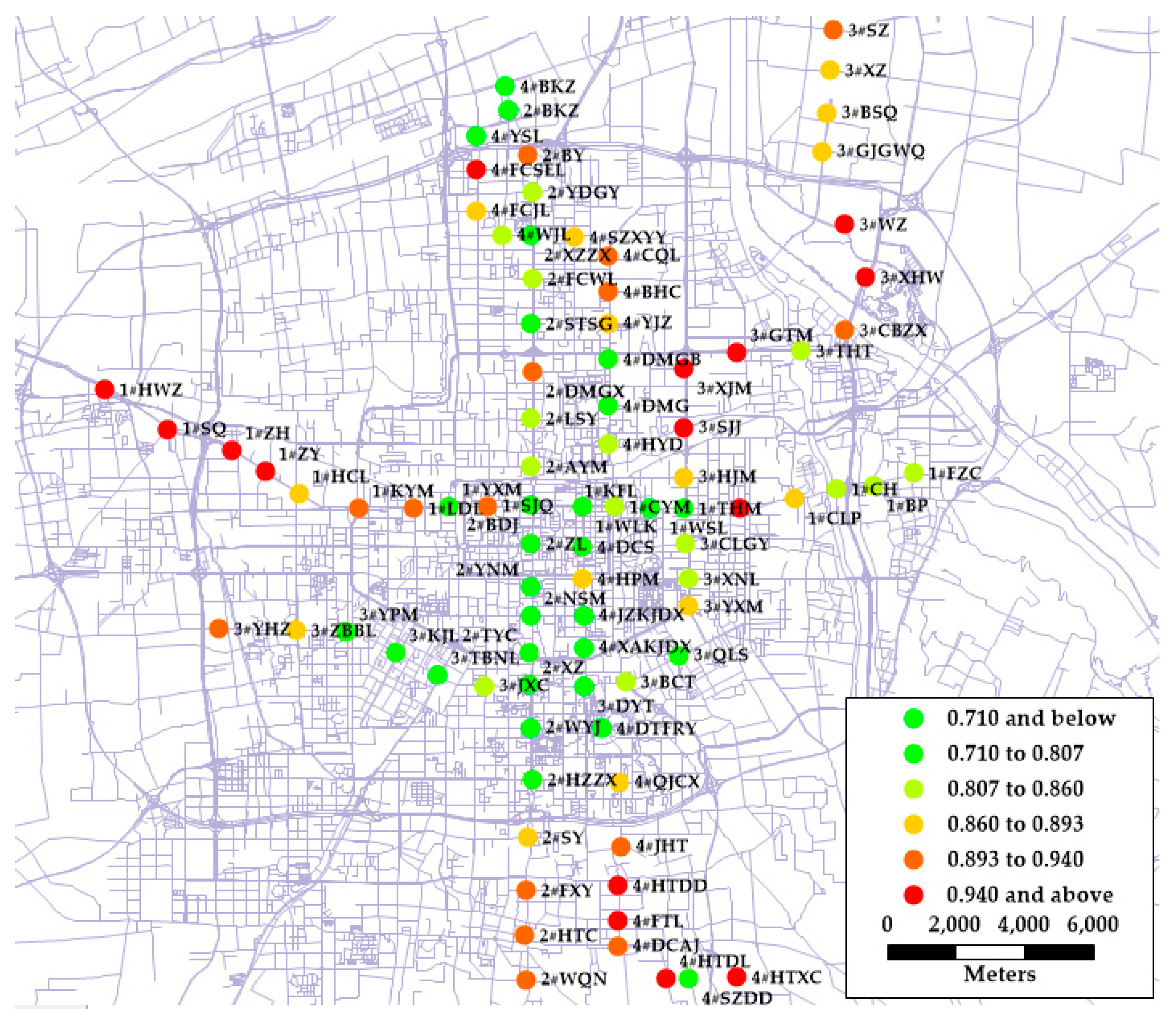
In China, only large cities have built up urban rail transit. The floating populations of these cities are large, and the populations around the stations are difficult to count. The high density of residential buildings can be attributed to more residents living near the stations [44]. Therefore, in this paper, the built environment is used in place of the population. In a study by Sung [45], the best catchment area for predicting station-level ridership is 500 m; thus, the statistical range of the current built environment is considered to be 500 m. The proportion of the commuting area as calculated by the built environment in a 500 m station catchment area is then used as an independent variable. The spatial distribution of the proportions of the commuting areas of Xi’an metro stations is presented in Figure 8.
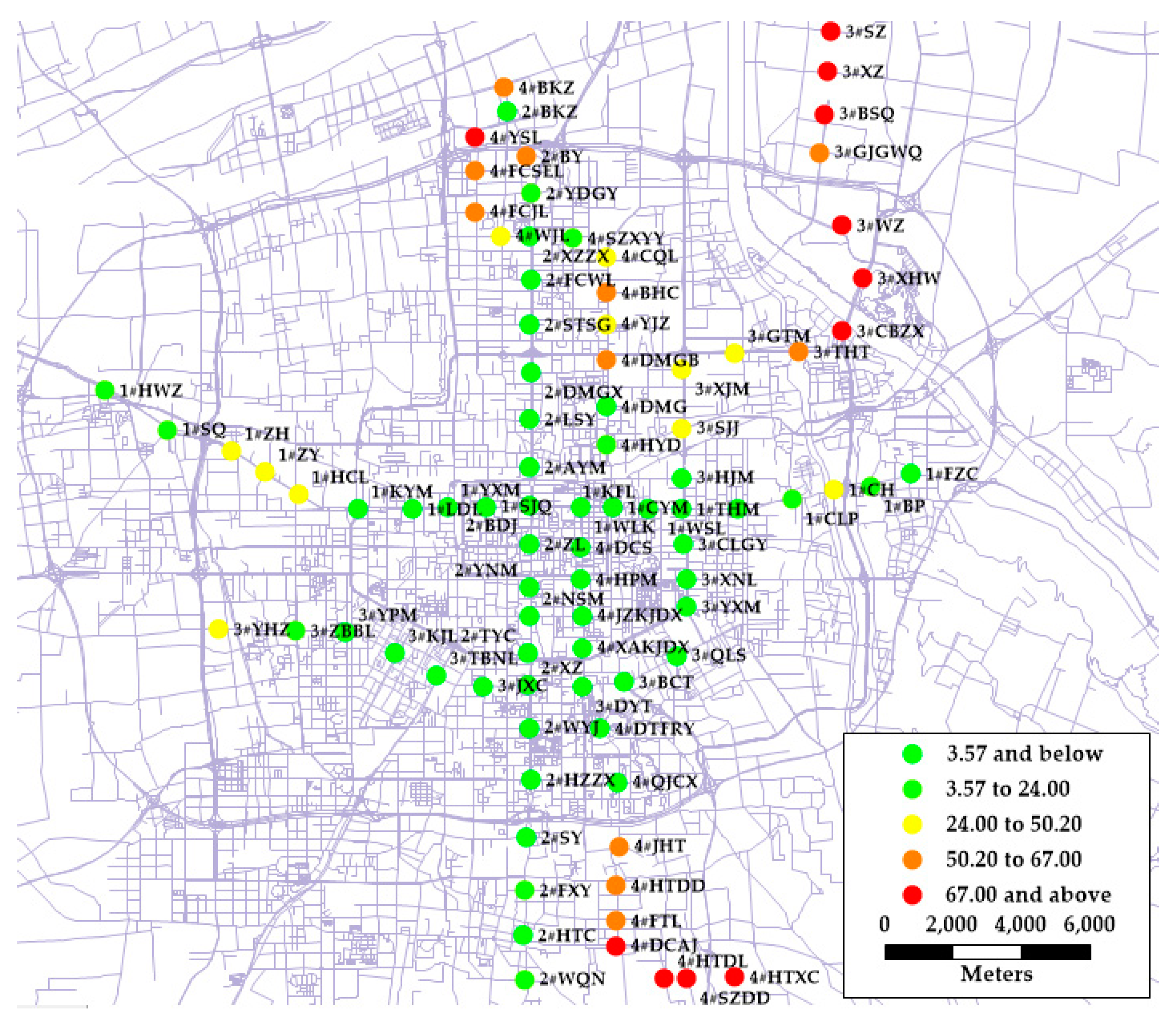
Yu [41] found that the area of undeveloped land around stations is related to the PDC, but no definite results were obtained. Thus, the undeveloped land area refers to the area of the undeveloped land around a station, and is used as an independent variable. The spatial distribution of undeveloped land areas of Xi’an metro stations is presented in Figure 9.
3.3.2. Distance to the City Center
García [46] determined that the location of a house (close to the sea or city center and located in a certain area) influenced housing prices. Therefore, properties in the same land-use class in different locations will have different prices, reflecting socioeconomic conditions in the area. If the metro station is far from the city center, people have to depart earlier because of the longer travel time. Thus, the distance to the city center is considered as an independent variable in this study.
3.3.3. Betweenness Centrality
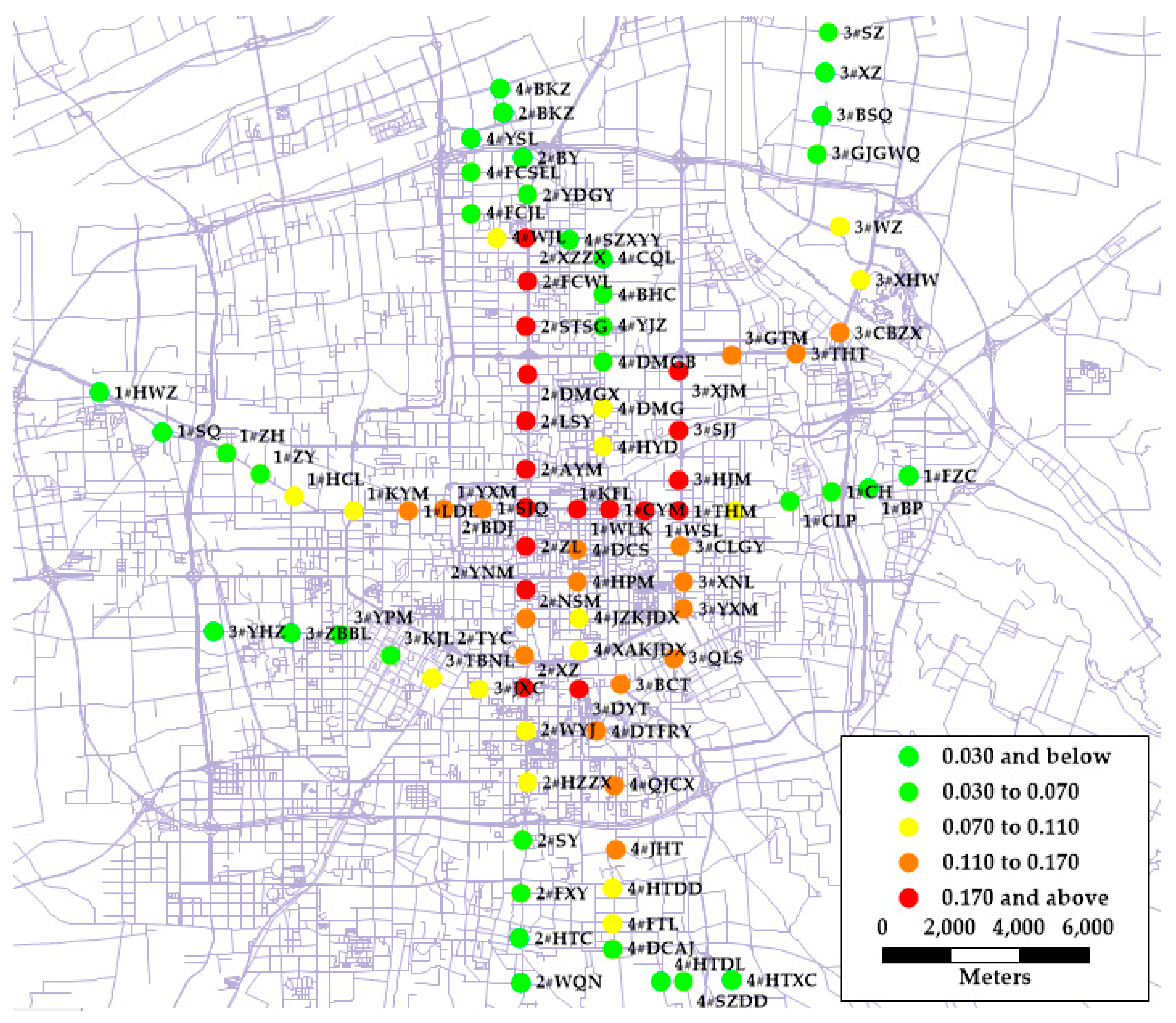
If the land use is the same at two stations, the ridership volume of a transfer station is higher than that of a normal station [47]. Existing studies have used these two types of stations as discrete dummy variables [48] when analyzing the differences between transfer stations and normal stations. However, this approach does not consider the differences between transfer stations in different locations. Therefore, the concept of betweenness centrality (BC), which is used in graph theory, is used in the present study to determine the locations and properties of stations in the urban rail transit network; the dummy variable indicates whether the station is a transfer station or not. There is one shortest path to every starting station s to terminal station t, but not all shortest paths pass through station i. The BC value reflects the situation of all shortest paths in the metro network that pass one station, and the formula is as follows:
where BCi is the betweenness centrality of station i, εsit is the number of shortest paths from station s to station t via station i, and εst is the number of shortest paths in the metro network from station s to station t.
The spatial distribution of the BC values of Xi’an metro stations is presented in Figure 10.
3.4. Summary of Variables
The variables used in this paper are described in Table 2.
4. Methodology
Based on the ordinary least square (OLS) model, the GWR model introduces local parameters to measure the spatial position, and the spatial characteristics of data are added into the model to show the local spatial characteristics and the instability of the spatial distribution in the research area [49]. The equation of the GWR model can be expressed as follows:
where PDCi is the PDC of metro station i, (ui, vi) denotes the location of station i, βk(ui, vi) indicates the kth regression parameter at station i, which is a function of the geographical position, and xik is the independent variable, of which there are four used in this study (the proportion of WPR, the undeveloped land area, the distance to the city center, and BC); their definitions and formulas were introduced in the previous chapter. Additionally, εi is the normally distributed error term of station i, and p is the total number of stations.
After omitting the spatial position term, the resulting equation is as follows:
Formula (4) can be expressed as:
The weighted least-squares method is used to minimize Formula (6) to calculate the regression parameters of station i:
where W(i) is the weight matrix of the geographically weighted regression at station i, and X is a matrix of explanatory variables. If the sample points of each station remain homogeneous in space, i.e., β(i) is a constant, then the GWR is equivalent to the OLS model. However, in actuality, the assumption of spatial independence or homogeneity is difficult to hold, especially in the related research of urban rail passenger flow; although the land use situation around each station is similar, due to the different spatial locations of each station, their boarding and alighting ridership are very different. It is clear that determining how to choose the desired spatial weight matrix is the key to accurately describing the spatial interaction, which largely determines the quality of the model fitting effect [50]. According to Hanham et al. [51], the Gaussian distance function was chosen in this study to be the basic form of space weight, and the expression is as follows:
where dij is the distance between station i and station j, and b is the kernel bandwidth parameter.
Point-by-point regression is performed by using the above method to obtain the regression parameter estimation matrix containing sample points:
Thus, the value of the dependent variable can be estimated as follows:
5. Results and Discussion
5.1. Spatial Autocorrelation and Local Collinearity Test
Before using the GWR model to analyze the relationship between PDC and the independent variables, the collinearity test of the independent variables must be done and one of the collinear variables must be deleted first. Table 3 shows the results of the collinearity test. According to the Mathematical dictionary [52], there are three methods to judge the collinearity of the independent variables. The condition index is more than 10, at least one of the variance ratios is close to 1, and the value of eigenvalue is 0. In Table 3, the condition index in the second line is more than 10, the variance ratio of the ‘distance to city center’ is 0.86, and the value of eigenvalue is 0.03. So this independent variable is deleted. The last line in Table 3 is the collinearity test result after deleting the ‘distance to city center’.
Before establishing the GWR model, the Moran I test must be conducted to determine if spatial autocorrelation exists. The results are shown in Table 4. The P-value of the variable is less than 0.05, and the Moran I is between −1 and 1. Thus, spatial autocorrelation exists, and the GWR model is suitable to setting up.
5.2. Results
5.2.1. Summary Statistics
The summary statistics of the local coefficients are shown in Table 5. If the Akaike information criterion (AIC) difference between the two models is greater than 3, the goodness of fit is considered to be significantly improved [44], and AIC is converted to corrected Akaike information criterion (AICc) in the case of a small sample. In Table 5, the AICc of GWR are decreased by more than 67 compared with the AICc of the OLS model. The adjusted R2 values are larger for the GWR (more than 0.8 for the PDCs) than for the OLS model. Cardozo [5] used the GWR model to forecast ridership at the metro station level. He used nine variables and the adjusted R2 value was 0.7. Thus, the adjusted R2 values in this paper are acceptable. The values of the undeveloped land area and BC are higher than 0, indicating that these variables have positive influences on the PDC. For the PDCa, the value of proportion of WPR is less than 0, demonstrating that the variable has a negative influence on the PDC, whereas for the PDCb, the value is near 0.
5.2.2. Spatial Distributions of the Coefficients
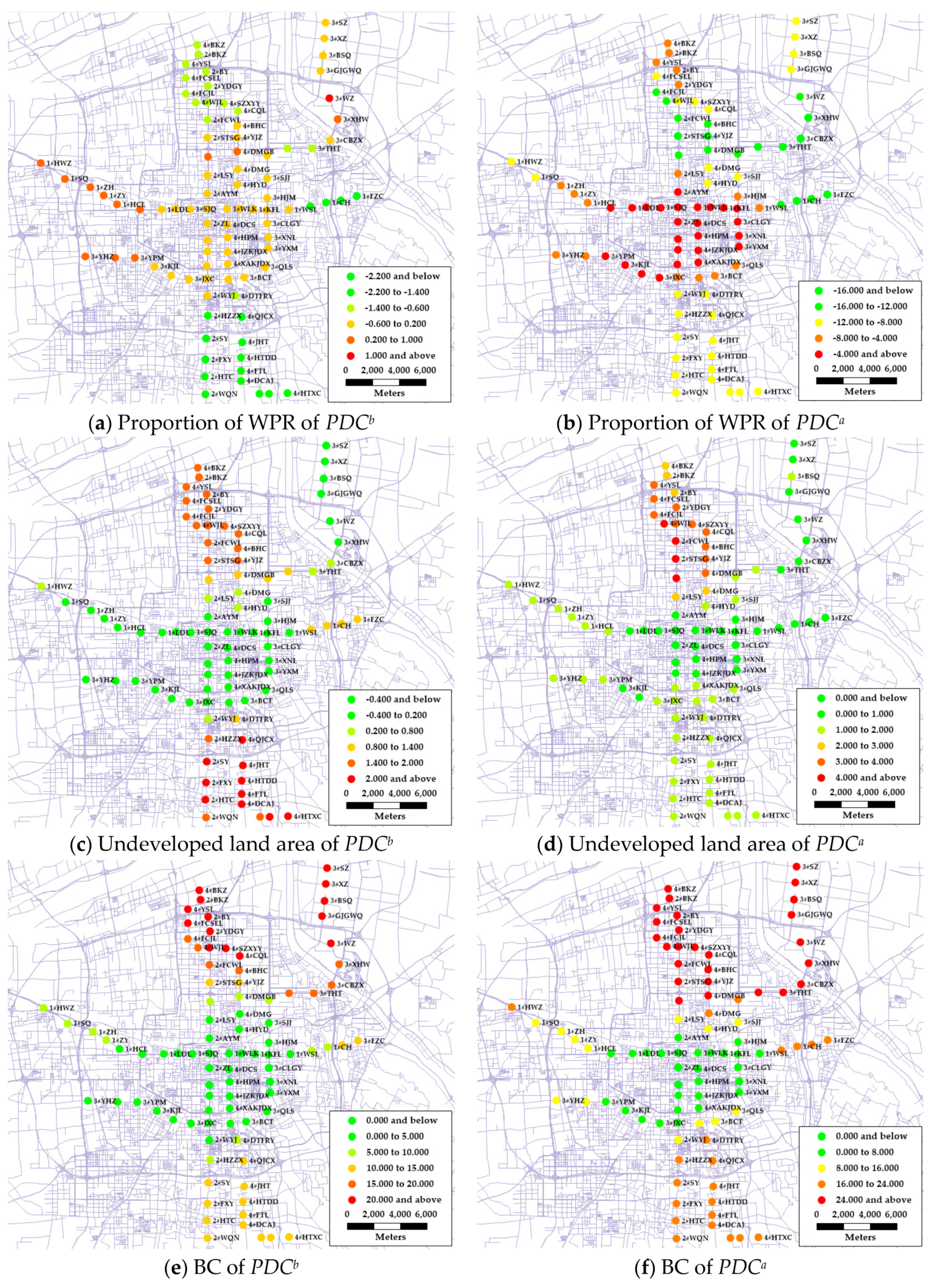
The spatial distributions of the regression coefficients are presented in Figure 11, from which it is evident that the spatial distributions of the same coefficients exhibit differences for different PDCs.
For the proportion of WPR, the regression coefficients of PDCb have both positive and negative numbers, and the values are small, ranging from −2.5 to 1.0. This demonstrates that this variable does not have a dominant influence on the PDC. For the spatial distribution of the proportion of WPR, the coefficients are close to 0.0 in the center and the northeast of the city, the coefficients are less than 0.0 in the north, south, and east of the city, and the coefficients are greater than 0.0 in the west of the city. In the northeast of the city, the land has not been maturely developed. In the north, south, and east of the city, there are three sub-centers near the stations 2#FCWL, 2#XZ, and 1#FZC. To the northwest of Xi’an, there is another city—Xianyang. The two cities are so close that the linear distance from 1#HWZ to the city center of Xianyang is only about 10 km. The office space in this area is uncertain, and the influences of the proportions of WPR on these stations are small. The regression coefficients of PDCa are all negative, indicating that the proportion of WPR has a negative influence on the PDC. The regression coefficients are higher in the city center and lower in the periphery. Because the regression coefficients are all negative, the influence increases from the center to the periphery.
For the undeveloped land area, the range of the PDCa values is slightly larger than that of the PDCb values. The spatial distributions are approximately the same, and the larger values occur in the periphery. By comparing Figure 9 and Figure 11c,d, it is clear that there are few stations in Metro Line 2 (the north–south line) that have undeveloped land, but the regression coefficients are substantially different. For the stations in the southeast and northeast of the city with large undeveloped land areas, the regression coefficients are still substantially different. This indicates that undeveloped land areas have uncertain influences on both the PDCb and PDCa values, which is consistent with the fact that trips to undeveloped land occur relatively seldom.
For the BC, the range of values is similar to those of the PDCb and the PDCa. Most values are positive, indicating that this variable has a positive influence on the PDC. The coefficients of the variables are smaller in the city center and larger in the periphery, which means that the BC has a greater influence on diverging a station’s peak hour from the city’s peak hour in suburban areas.
5.2.3. Station Classification
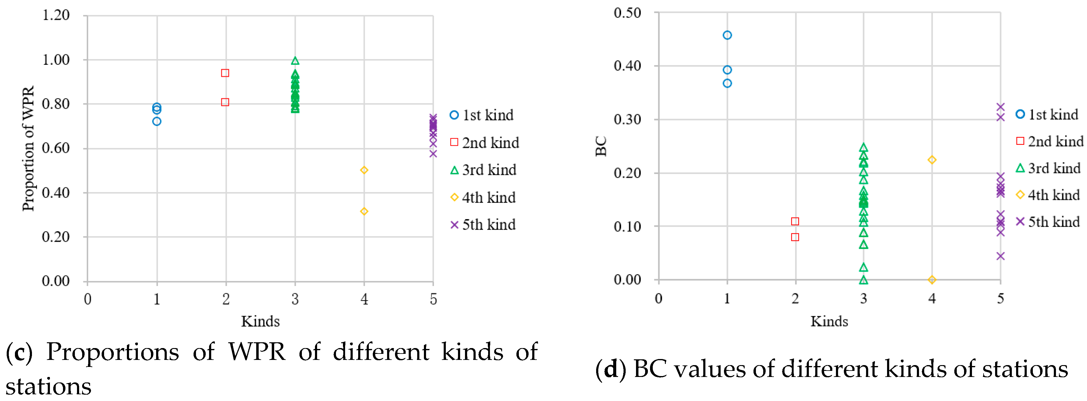
Because the undeveloped land area has an uncertain influence on the PDC, the k-means method was used to classify stations with undeveloped land areas of 0. The classifying variables are the proportion of WPR, BC, PDCb, and PDCa, and the results are presented in Table 6 and Figure 12. The PDCb and PDCa values in the 1st, 3rd, and 5th kinds of stations are all less than 1.17, and the proportions of WPR in these kinds of stations are all greater than 0.5, indicating that lands for work, primary and middle schools, and residences of these stations occupies the main body. However, the BC values in these kinds of stations are different. The BC values in the 1st kind of station are greater than 0.35, indicating that these stations are in important positions of the metro network; most of the BC values in the 3rd and 5th kinds of stations are less than 0.3, and fall within a wide range. The PDCa values in the 4th kind of station are greater than 1.13, and the PDCb values are very large. The values of the proportion of WPR in the 4th kind of station are less than 0.5, indicating that other land of these stations occupies the main body. The BC values in this kind of station are within a large range from 0 to 0.2. For the 2nd kind of station, the proportion of WPR is greater than 0.8, and the BC is about 0.1, meaning that these stations are commuting stations and not in very important areas. The PDCb values are close to 1, but the PDCa values are the greatest among all the PDCa values. There are two stations of the 2nd kind, namely 1#KYM and 4#DMG. 1#KYM has a large amount of industrial land and many residential districts established by a factory manager, and these lands do not produce medium- or long-distance travel. 4#DMG is near cultural relics and historic sites, including Daming Palace National Heritage Park, but this area is not as developed as the Greater Wild Goose Pagoda Square, and the station only sees 276 people during the city’s peak hour and 340 people during the station’s peak hour.
Thus, the proportion of WPR has the greatest influence on the PDC. If the proportion of WPR is less than 0.5, the PDCb and PDCa values are both very large; if the proportion of WPR is greater than 0.5, most PDCb and PDCa values are close to 1.
5.3. Discussion—Future Station Design and Policy
The enlargement coefficient put forward in this paper, PDC, can be used as a simple way to convert the ridership during a city’s peak hour to the ridership during a station’s peak hour. The proportion of the WPR was found to have a negative influence on the PDCa value. In other words, the larger the lands for work, primary and middle schools, and residences, the smaller the deviation of ridership between a station’s peak hour and the city’s peak hour, as the commuting trip during workdays constitutes the city’s peak hour. This result is consistent with the results of previous studies [8,53] that investigated the metro ridership in Osaka, Shanghai, and Zhengzhou, and found that trips of going to work and going to school make the station’s peak hour earlier, while shopping and traveling trips delay the station’s peak hour.
If the proportion of WPR of a station is greater than 0.5, it can be considered that the ridership during the city’s peak hour is the highest ridership of the whole day; if it is less than 0.5, the highest ridership is the ridership during the city’s peak hour multiplied by the PDC. This result is consistent with the findings of Yu [41], who examined two cities—Xi’an and Chongqing—and found that the PDC value of most metro stations is close to 1 when the proportion of WPR is greater than 0.5.
In the morning, the proportion of WPR has more influence on the alighting ridership than on the boarding ridership. For stations with proportions of WPR of greater than 0.5, if it is a special type of land, such as the 1#KYM and 4#DMG stations, the PDCb value is close to 1, but the PDCa value is greater among the PDCa values of all stations. Moreover, the regression coefficients of PDCa are negative, but the regression coefficients of PDCb are both positive and negative numbers. This means that the proportion of WPR results in the alighting ridership occurring during a city’s peak hour, but does not have a clear effect on the boarding ridership. It indicates that the lands for work, primary and middle schools, and residences has more explanatory power regarding the peak hour deviation in the alighting during morning peak hours. The lands for work, primary and middle schools mostly attract office workers and students who need to arrive on time or ahead of schedule. Compared with their boarding behavior, their alighting behavior has a relatively clear arrival time. For different enterprises or schools, the time is almost the same, and is the same as the city’s peak hour. However, the boarding times will present large differences because of the distance between home and work. In China, the administrative land is more concentrated than residential land [54], which will lead to the concentrated distribution of commuting–alighting passenger flow.
The local coefficient of BC is greater than 0, meaning it has an influence on the deviation of the peak hours of the station and city. For the spatial distribution, the BC is greater in suburban areas, indicating that the BC has a greater influence on diverging a station’s peak hour from the city’s peak hour in suburban areas. This is because commuters who live in suburban areas and work in the city center need to leave earlier. This finding is reasonable, as housing prices in suburban areas are lower; people are more willing to live in these areas, thus increasing their time spent on the metro and affecting the station’s peak hour. This evidence is consistent with the results of previous studies [43], which found that more people want to live in suburban areas, resulting in the increased metro travel demands of these areas.
In China, station design must consider the extra peak hour passenger flow, which is the predicted peak hour passenger flow multiplied by the extra peak hour factor, which is between 1.1 and 1.4 [2]. The extra peak hour factor (EPHF) is the highest fifteen-minute ridership during the city’s peak hour multiplied by 4, and then divided by the ridership during the city’s peak hour [55]. The EPHF is the expanded threshold of the station’s capacity in the city’s peak hour. However, this study shows that some stations’ own peak hours are inconsistent with the city’s peak hour because of various land use and BC around the stations, and the peak load shifting is formed. This results in that the EPHF does not have constraints to these peak load shifting stations’ capacities. Thus, this paper put forward the PDC to depict this inconsistent phenomenon of the station’s peak hour. Although the EPHF and the PDC both reflect the temporal distribution of metro stations, they are totally different. The EPHF reflects the concentration of passenger flow in a city’s peak hour, while the PDC reflects the inconsistency between a station’s peak hour and the city’s peak hour. There is no comparability between the two coefficients. Moreover, the thinking methods about the EPHF and the PDC are completely different from each other. For example, stations with large proportions of administrative land usually have high EPHF values because of the instantaneous gathering of commuting ridership [56]. But the greater commuting ridership results in the high consistency between the station’s peak hour and that of the city, leading to a PDC value close to 1. By contrast, stations with large proportions of commercial land usually have low EPHF values because of the randomness of the shopping flow [57]. However, the peak hour of shopping flow lags behind the city’s peak hour, leading to the station’s peak hour being highly inconsistent with the city’s, and this increases the PDC value. Thus, there are two ridership options when designing stations, namely the extra peak hour ridership during a city’s peak hour and ridership during a station’s peak hour.
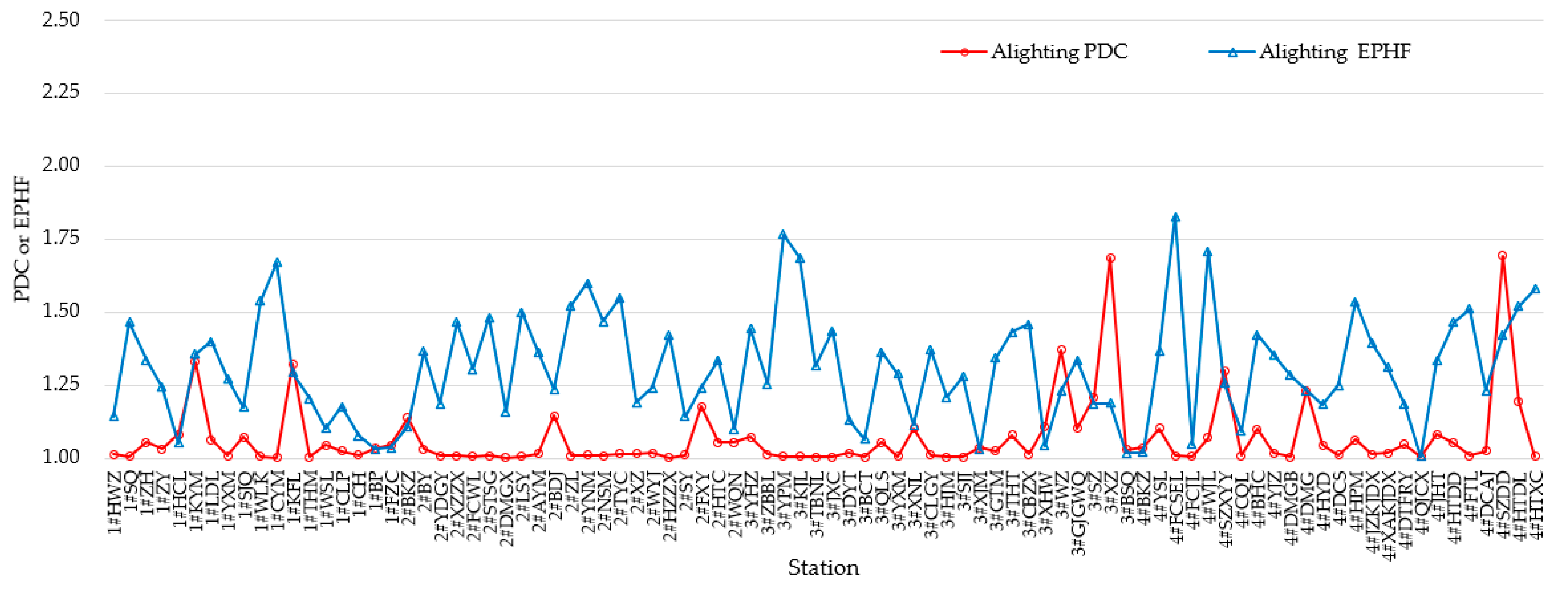
The morning boarding and alighting PDC and EPHF values of Xi’an metro stations are shown in Figure 13 and Figure 14. The fluctuations of the PDC and the EPHF values are different. For the boarding ridership, the EPHF values change from 1.1 to 1.5, while most PDC values are about 1.0. However, five stations’ PDC values are greater than 1.8, and nine stations’ PDC values are greater than their EPHF values. For the alighting ridership, the EPHF values change from 1.0 to 1.8, while most PDC values are about 1.0, but fifteen stations’ PDC values are greater than their EPHF values. Therefore, the size relationship between the extra peak hour passenger flow during a city’s peak hour and the ridership during a station’s peak hour cannot be determined. If only one kind of coefficient is used to design the station, the scale of some of the station will be small. Thus, when a station is designed, both types of ridership (the extra peak hour ridership during a city’s peak hour and ridership during a station’s peak hour) must be calculated, and the larger of the two is used to design the station.
The land development in the center of Xi’an has been completed, and the city is now faced with land replacement and land development in urban areas. Land replacement refers to moving industrial land from the city center to urban areas and changing the land to other types of property. Non-commuting land can mitigate the traffic pressure of a city’s peak hour, because its travel peak is different from that of commuting land. However, the mixed land use ratio must be considered. More non-commuting land around metro stations will result in the deviation of their peak hours from those of the city. This will increase the difficulty of both passenger flow forecasting in the planning stage and train departure intervals and station management in the operation stage. Because there is only one train departure interval in a period of time in a section of a metro line, if a station’s peak hour is different from that of other stations, the train departure interval will be greater in this station‘s peak hour, and passengers will pile up. However, less non-commuting land around metro stations will result in a large extra peak hour passenger flow and a small off-peak hour passenger flow. Although a significant amount of money may be spent on building a large station, it may be nearly empty for most of the day. Thus, the proportion of commuting land around metro stations must be considered in land planning.
6. Conclusion
In this study, we investigated the differences in the ridership of metro stations between the stations’ peak hours and the city’s peak hours for 88 metro stations in Xi’an. The enlargement coefficient put forward in this paper, PDC, can be used as a simple way to convert the ridership during a city’s peak hour to the ridership during a station’s peak hour. GWR was used to determine the influencing factors on the ridership volume and specifically on the PDC. The key findings are as follows:
The proportion of WPR is found to have a negative influence on the PDCa value. In the morning, the proportion of WPR has more influence on the alighting ridership than on the boarding ridership. If the proportion of WPR of a station is greater than 0.5, it can be considered that the ridership during the city’s peak hour is the highest ridership of the whole day; if it is less than 0.5, the highest ridership is the ridership during the city’s peak hour multiplied by the PDC.
The BC has an influence on the deviation of the peak hours of the station and city, and the BC is greater in suburban areas, indicating that the BC has a greater influence on diverging a station’s peak hour from the city’s peak hour in suburban areas.
Thus, if a metro station is primarily surrounded by commuting land (such as if the proportion of commuting land area is greater than 0.5 in Xi’an), does not have special land (such as an external transportation hub), and is located in the city center, its PDC is close to 1.
When designing a metro station, there are two ridership options, namely the extra peak hour ridership during a city’s peak hour and ridership during a station’s peak hour. The size relationship between the extra peak hour passenger flow during a city’s peak hour and the ridership during a station’s peak hour cannot be determined. The larger of the two is used to design the station. However, for the stations to accord with the conditions in the previous paragraph, they only need to consider the extra peak hour factor, as their values of PDC are close to 1.
When performing urban land use planning, the mixed land use ratio must be considered. Non-commuting land can mitigate the traffic pressure of a city’s peak hour, but at the same time more non-commuting land around metro stations will result in the deviation of their peak hours from those of the city. This will increase the difficulty of both passenger flow forecasting in the planning stage and train departure intervals and station management in the operation stage.
The transfer passenger volume cannot be counted by the automatic fare collection system directly, and its correctness cannot be verified. Thus, this research only considered the boarding and alighting volumes, and did not account for transfer passengers in interchange stations; an inconsistent peak hour phenomenon also occurs for transfer passengers, which would influence the design of transfer channels. Therefore, this topic will be investigated in future research.
Author Contributions
Conceptualization, L.Y.; methodology, Y.C.; software, Y.C.; validation, L.Y.; formal analysis, L.Y. and K.C.; investigation, L.Y.; resources, K.C.; data curation, Y.C.; writing—original draft preparation, L.Y.; writing—review and editing, Y.C.; visualization, Y.C.; funding acquisition, K.C. All authors have read and agreed to the published version of the manuscript.
Funding
This research was funded by the National Natural Science Foundation of China, grant number 71871027.
Acknowledgments
We would like to acknowledge the anonymous reviewers and the authors of the cited papers for their detailed comments, without which this work would not have been possible.
Conflicts of Interest
The authors declare no conflict of interest.
References
- Kittelson, J. Associates, Parsons Brinckerhoff, KFH Group. Transit Capacity and Quality of Service Manual, 3rd ed.; Transportation Research Board: Washington, DC, USA, 2013. [Google Scholar]
- GB50157-2013. Code for Design of Metro. Available online: http://www.jianbiaoku.com/webarbs/book/1027/1073295.shtml (accessed on 13 February 2020).
- Ma, C.Q.; Wang, Y.P. Traffic volume forecast for xi’an urban rapid rail transit. Urban Rapid Rail Transit 2006, 19, 24–28. [Google Scholar]
- Mwakalonge, J.L. Econometric Modeling of Total Urban Travel Demand Using Data Collected in Single and Repeated Cross-Sectional Surveys. Ph.D. Thesis, Tennessee Technological University, Cookeville, TN, USA, May 2010. [Google Scholar]
- Cardozo, O.D.; Garcia-Palomares, J.C.; Gutierrez, J. Application of geographically weighted regression to the direct forecasting of transit ridership at station-level. Appl. Geogr. 2012, 34, 548–558. [Google Scholar] [CrossRef]
- Michael, G.M. The Four Step Model. In Handbook of Transport Modeling; Emerald Group Publishing Limited: Bingley, UK, 2007. [Google Scholar]
- Cui, Z.J. On Scale of Subway Station Platform. J. Southwest Jiaotong Univ. 1993, 3, 76–80. [Google Scholar]
- Gu, L.P.; Ye, X.F. Study on the in and out passenger flow during peak hours of the rail transit station in Osaka. Compr. Transp. 2014, 2, 57–61. [Google Scholar]
- GB/T51150-2016. Code for Prediction of Urban Rail Transit Ridership. Available online: http://www.zzguifan.com/webarbs/book/92970/3172164.shtml (accessed on 13 February 2020).
- Tobin, R.L.; Friesz, T.L. Sensitivity analysis for equilibrium network flow. Transp. Sci. 1988, 22, 100–105. [Google Scholar] [CrossRef]
- Vovsha, P. Application of cross-nested logit model to mode choice in Tel Aviv, Israel, metropolitan area. Transp. Res. Rec. 1997, 1607, 6–15. [Google Scholar] [CrossRef]
- Sun, X.; Wilmot, C.G.; Kasturi, T. Household travel, household characteristics, and land use: An empirical study from the 1994 Portland activity-based travel survey. Transp. Res. Rec. 1998, 1617, 10–17. [Google Scholar] [CrossRef]
- Yam, R.C.M.; Whitfield, R.C.; Chung, R.W.F. Forecasting traffic generation in public housing estates. J. Transp. Eng. 2000, 126, 358–361. [Google Scholar] [CrossRef]
- Rezaeestakhruie, H. Analytical error propagation in four-step transportation demand models. Comput. Sci. 2017. [Google Scholar] [CrossRef]
- Sanko, N.; Morikawa, T.; Nagamatsu, Y. Post-project evaluation of travel demand forecasts: Implications from the case of a Japanese railway. Transp. Policy 2013, 27, 209–218. [Google Scholar] [CrossRef]
- Ryu, S.; Chen, A.; Zhang, H.M. Path flow estimator for planning applications in small communities. Transp. Res. Part A Policy Pract. 2014, 69, 212–242. [Google Scholar] [CrossRef] [Green Version]
- Cervero, R.; Murakami, J.; Miller, M. Direct ridership model of bus rapid transit in Los Angeles County, California. Transp. Res. Rec. 2010, 2145, 1–7. [Google Scholar] [CrossRef] [Green Version]
- Feng, X.; Sun, Q.; Liu, J. Time Characteristic of Input Passenger in Urban Rail Transit Stations Among High Density Residential Areas. In Proceedings of the Chinese Control Conference, Beijing, China, 29–31 July 2010. [Google Scholar]
- Dend, J.; Xu, M. Characteristics of subway station ridership with surrounding land use: A case study in Beijing. In Proceedings of the 2015 International Conference on Transportation Information and Safety (ICTIS), Wuhan, China, 25–28 June 2015. [Google Scholar]
- Chen, C.; Chen, J.; Barry, J. Diurnal pattern of transit ridership: A case study of the New York City subway system. J. Transp. Geogr. 2009, 17, 176–186. [Google Scholar] [CrossRef]
- Chan, S.; Miranda-Moreno, L. A station-level ridership model for the metro network in Montreal, Quebec. Can. J. Civ. Eng. 2013, 40, 254–262. [Google Scholar] [CrossRef]
- Choi, J.; Lee, Y.J.; Kim, T. An analysis of Metro ridership at the station-to-station level in Seoul. Transportation 2012, 39, 705–722. [Google Scholar] [CrossRef]
- Sung, H.; Oh, J.T. Transit-oriented development in a high-density city: Identifying its association with transit ridership in Seoul, Korea. Cities 2011, 28, 70–82. [Google Scholar] [CrossRef]
- He, Y.X.; Zhao, Y.; Tsui, K.L. Modeling and analyzing spatiotemporal factors influencing metro station ridership in taipei: An approach based on general estimating equation. arXiv 2019, arXiv:1904.01280. [Google Scholar]
- Roos, J.; Bonnevay, S.; Gavin, G. Short-Term Urban Rail Passenger Flow Forecasting: A Dynamic Bayesian Network Approach. In Proceedings of the 2016 15th IEEE International Conference on Machine Learning and Applications (ICMLA), Anaheim, CA, USA, 18–20 December 2016. [Google Scholar]
- Haire, A.R. A methodology for incorporating fuel price impacts into short-term transit ridership forecasts. Ph.D. Thesis, The University of Texas at Austin, Austin, TX, UAS, May 2009. [Google Scholar]
- Ma, X.L.; Zhang, J.Y.; Du, B. Parallel Architecture of Convolutional Bi-Directional LSTM Neural Networks for Network-Wide Metro Ridership Prediction. IEEE Trans. Intell. Transp. Syst. 2018, 99, 1–11. [Google Scholar] [CrossRef]
- Li, B. Research on the Computer Algorithm Application in Urban Rail Transit Holiday Passenger Flow Prediction. In Proceedings of the 2016 International Conference on Network and Information Systems for Computers, Wuhan, China, 15–17 April 2016. [Google Scholar]
- Yang, R.; Wu, B. Short-term passenger flow forecast of urban rail transit based on BP neural network. In Proceedings of the Intelligent Control & Automation, Jinan, China, 7–9 July 2010. [Google Scholar]
- Shen, J.Y. Simplified calculation for the width of on and off region of station platform. Urban Rapid Rail Transit 2008, 05, 9–12. [Google Scholar]
- Chen, K.M.; Yu, L.J.; Ma, C.Q. Differentiated peak hours at urban rail transit stations in Xi’an. Urban Transp. China 2018, 16, 51–58. [Google Scholar]
- Ping, S.H. Characteristics of temporal passenger flow distribution at different stations on shenzhen metro line 1. Urban Mass Transit 2018, 21, 85–87. [Google Scholar]
- Brunsdon, C.; Fotheringham, A.S.; Charlton, M.E. Geographically weighted regression: A method for exploring spatial non stationarity. Geogr. Anal. 1996, 28, 281–298. [Google Scholar] [CrossRef]
- Chen, E.; Ye, Z.; Wang, C. Discovering the spatio-temporal impacts of built environment on metro ridership using smart card data. Cities 2019, 95, 102359. [Google Scholar] [CrossRef]
- Hadayeghi, A.; Shalaby, A.S.; Persaud, B.N. Development of planning level transportation safety tools using geographically weighted poisson regression. Accid. Anal. Prev. 2010, 42, 676–688. [Google Scholar] [CrossRef] [PubMed]
- Clark, S.D. Estimating local car ownership models. J. Transp. Geogr. 2007, 15, 184–197. [Google Scholar] [CrossRef] [Green Version]
- Zhao, F.; Park, N. Using geographically weighted regression models to estimate annual average daily traffic. J. Transp. Res. Board 2004, 1879, 99–107. [Google Scholar] [CrossRef]
- Qian, X.; Ukkusuri, S.V. Spatial variation of the urban taxi ridership using GPS data. Appl. Geogr. 2015, 59, 31–42. [Google Scholar] [CrossRef]
- Paez, A. Exploring contextual variations in land use and transport analysis using a probit model with geographical weights. J. Transp. Geogr. 2006, 14, 167–176. [Google Scholar] [CrossRef]
- Blainey, S.P.; Preston, J.M. A geographically weighted regression based analysis of rail commuting around Cardiff, South Wales. In Proceedings of the 12th World Conference on Transportation Research, Lisbon, Portugal, 11–15 July 2010. [Google Scholar]
- Yu, L.; Chen, Q.; Chen, K. Deviation of peak hours for urban rail transit stations: A case study in Xi’an, China. Sustainability 2019, 11, 2733. [Google Scholar] [CrossRef] [Green Version]
- Kong, X.; Yang, J. A new method for forecasting station-level transit ridership from land-use perspective: The case of shenzhen city. Sci. Geogr. Sin. 2018, 38, 2074–2083. [Google Scholar] [CrossRef]
- Zhao, J.; Deng, W.; Song, Y. Analysis of Metro ridership at station level and station-to-station level in Nanjing: An approach based on direct demand models. Transportation 2014, 41, 133–155. [Google Scholar] [CrossRef]
- Zhu, Y.; Chen, F.; Wang, Z. Spatio-temporal analysis of rail station ridership determinants in the built environment. Transportation 2019, 46, 2269–2289. [Google Scholar] [CrossRef]
- Sung, H.; Choi, K.; Lee, S. Exploring the impacts of land use by service coverage and station-level accessibility on rail transit ridership. J. Transp. Geogr. 2014, 36, 134–140. [Google Scholar] [CrossRef]
- García, P.A. Several determinant factors of the secondhand housing price: An application of the hedonic methodology. Rev. Estud. Reg. 2008, 82, 135–158. [Google Scholar]
- Gutiérrez, J.; Cardozo, O.-D.; García-Palomares, J.-C. Transit ridership forecasting at station level: An approach based on distance-decay weighted regression. J. Transp. Geogr. 2011, 19, 1081–1092. [Google Scholar] [CrossRef]
- Report 16 Transit and Urban Form. Available online: http://onlinepubs.trb.org/onlinepubs/tcrp/tcrp_rpt_16-2.pdf (accessed on 13 February 2020).
- Fotheringham, A.S.; Brunsdon, C.; Charlton, M.E. Geographically Weighted Regression: The Analysis of Spatially Varying Relationships; Wiley: Hoboken, NJ, USA, 2002. [Google Scholar]
- Brunsdon, C.; Fotheringham, A.S.; Charlton, M. Geographically weighted summary statistics-a framework for localised exploratory data analysis. Comput. Environ. Urban Syst. 2002, 26, 501–524. [Google Scholar] [CrossRef] [Green Version]
- Hanham, R.; Hoch, R.J.; Spiker, J.S. The Spatially Varying Relationship Between Local Land-Use Policies and Urban Growth: A Geographically Weighted Regression Analysis. In Planning and Socioeconomic Applications; Springer: Berlin/Heidelberg, Germany, 2009. [Google Scholar]
- Wang, Y.; Wen, L.; Chen, M.F. Mathematical Dictionary; Science Press: Beijing, China, 2010. [Google Scholar]
- Zhao, X.F.; Tong, X.J. Characteristic analysis of temporal and spatial distributions of passengers on zhengzhou metro line 1. Urban Mass Transit 2017, 20, 75–79. [Google Scholar]
- Ma, X.; Liu, C.; Wen, H.; Wang, Y.; Wu, Y.J. Understanding commuting pattern using transit smart card data. J. Transp. Geogr. 2017, 58, 135–145. [Google Scholar] [CrossRef]
- Bassan, S. Modeling of peak hour factor on highways and arterials. KSCE J. Civ. Eng. 2013, 17, 224–232. [Google Scholar] [CrossRef]
- Jin, Y. Characteristics of peak hour passenger flow at rail transit stations in shanghai. Urban Transp. China 2019, 17, 50–57. [Google Scholar]
- He, J. Study on the configuration quantity of automatic ticket checker in urban rail transit. Railw. Signal. Commun. 2008, 44, 14–17. [Google Scholar]
Figure 1.
Land use of Xi’an metro stations (*104 m2).

Figure 2.
Time distribution of metro station 1#CLP in the morning.

Figure 3.
Time distribution of metro station 2#BKZ in the morning.

Figure 4.
Time distribution of metro station 3#DYT in the morning.

Figure 5.
The morning boarding ridership in the peak hours of the city and stations, and the PDC values of Xi’an metro stations.
Figure 5.
The morning boarding ridership in the peak hours of the city and stations, and the PDC values of Xi’an metro stations.

Figure 6.
The morning alighting ridership in the peak hours of the city and stations, and the PDC values of Xi’an metro stations.
Figure 6.
The morning alighting ridership in the peak hours of the city and stations, and the PDC values of Xi’an metro stations.

Figure 7.
Temporal distribution of trip purposes in Xi’an.

Figure 8.
Spatial distribution of the proportions of work, primary and middle schools, and residences (WPR) of Xi’an metro stations.
Figure 8.
Spatial distribution of the proportions of work, primary and middle schools, and residences (WPR) of Xi’an metro stations.

Figure 9.
Spatial distribution of the undeveloped areas of Xi’an metro stations.

Figure 10.
Spatial distribution of the betweenness centrality (BC) values of Xi’an metro stations.

Figure 11.
Spatial distribution of regression coefficients.

Figure 12.
The values of variables for different kinds of stations.


Figure 13.
The morning boarding PDC and EPHF values of Xi’an metro stations.

Figure 14.
The morning alighting PDC and EPHF values of Xi’an metro stations.


Table 1.
The statistical peak deviation coefficient (PDC) in Chongqing, China.
| Range | Morning PDC | Evening PDC | ||
|---|---|---|---|---|
| Data | Ratio | Data | Ratio | |
| (1.00, 1.10) | 37 | 71.15% | 34 | 65.38% |
| (1.10, 1.20) | 11 | 21.15% | 11 | 21.15% |
| (1.20, 1.30) | 3 | 5.77% | 2 | 3.85% |
| (1.30, 1.40) | 0 | 0.00% | 1 | 1.92% |
| (1.40, +∞) | 1 | 1.92% | 4 | 7.69% |
Table 2.
The variables used in this paper.
| Variable | Explanation | Value | ||
|---|---|---|---|---|
| Mean | Max | Min | ||
| PDCb | Dimensionless continuous values | 1.134 | 3.990 | 1.000 |
| PDCa | Dimensionless continuous values | 1.068 | 1.693 | 1.000 |
| Proportion of WPR | Dimensionless continuous values | 0.764 | 0.995 | 0.062 |
| Undeveloped land | Unit: 104 km2 | 22.778 | 76.516 | 0.000 |
| Distance to the city center | Continuous values, unit: km | 7.561 | 17.800 | 0.200 |
| BC | Dimensionless continuous values | 0.113 | 0.457 | 0.000 |
Table 3.
Collinearity test result.
| Eigenvalue | Condition Index | Variance ratio | |||
|---|---|---|---|---|---|
| Proportion of WPR | Distance to City Center | Undeveloped Land Area | BC | ||
| 0.03 | 11.58 | 0.17 | 0.86 | 0.23 | 0.50 |
| 0.10 | 5.40 | 0.29 | - | 0.41 | 0.46 |
Table 4.
Moran I test results.
| Variable | Moran I | Expectation Index | Mean Value | Z-score | P-value |
|---|---|---|---|---|---|
| Proportion of WPR | 0.099 | −0.012 | −0.011 | 1.788 | 0.044 |
| Undeveloped land area | 0.548 | −0.012 | −0.010 | 8.476 | 0.001 |
| BC | 0.523 | −0.012 | −0.008 | 6.610 | 0.001 |
Table 5.
Statistics of the local coefficients.
| Model | Dependent Variable | Corrected Akaike Information Criterion (AICc) | Adjusted R2 | Proportion of WPR | Undeveloped Land Area | BC |
|---|---|---|---|---|---|---|
| Ordinary least square (OLS) | PDCb | 700.068 | 0.522 | −0.777 | 1.433 | 14.038 |
| PDCa | 643.217 | 0.750 | −14.110 | 2.013 | 23.630 | |
| Geographically weighted regression (GWR) | PDCb | 607.986 | 0.860 | −0.611 | 0.752 | 8.955 |
| PDCa | 575.484 | 0.900 | −8.184 | 1.419 | 15.182 |
Table 6.
Summary statistics of the local coefficients.
| Variables | 1st Kind | 2nd Kind | 3rd Kind | 4th Kind | 5th Kind | |
|---|---|---|---|---|---|---|
| PDCb | Mean | 1.171 | 1.006 | 1.010 | 3.635 | 1.036 |
| Max | 1.309 | 1.008 | 1.034 | 3.990 | 1.186 | |
| Min | 1.001 | 1.004 | 1.001 | 3.281 | 1.000 | |
| PDCa | Mean | 1.051 | 1.280 | 1.025 | 1.230 | 1.014 |
| Max | 1.143 | 1.328 | 1.101 | 1.323 | 1.047 | |
| Min | 1.004 | 1.232 | 1.000 | 1.137 | 1.004 | |
| Proportion of WPR | Mean | 0.759 | 0.871 | 0.854 | 0.410 | 0.685 |
| Max | 0.786 | 0.936 | 0.995 | 0.503 | 0.739 | |
| Min | 0.721 | 0.805 | 0.777 | 0.317 | 0.575 | |
| BC | Mean | 0.405 | 0.094 | 0.143 | 0.113 | 0.160 |
| Max | 0.457 | 0.108 | 0.248 | 0.225 | 0.323 | |
| Min | 0.367 | 0.079 | 0.000 | 0.000 | 0.045 | |
© 2020 by the authors. Licensee MDPI, Basel, Switzerland. This article is an open access article distributed under the terms and conditions of the Creative Commons Attribution (CC BY) license (http://creativecommons.org/licenses/by/4.0/).
Share and Cite
MDPI and ACS Style
Yu, L.; Cong, Y.; Chen, K. Determination of the Peak Hour Ridership of Metro Stations in Xi’an, China Using Geographically-Weighted Regression. Sustainability 2020, 12, 2255. https://0-doi-org.brum.beds.ac.uk/10.3390/su12062255
AMA Style
Yu L, Cong Y, Chen K. Determination of the Peak Hour Ridership of Metro Stations in Xi’an, China Using Geographically-Weighted Regression. Sustainability. 2020; 12(6):2255. https://0-doi-org.brum.beds.ac.uk/10.3390/su12062255
Chicago/Turabian StyleYu, Lijie, Yarong Cong, and Kuanmin Chen. 2020. "Determination of the Peak Hour Ridership of Metro Stations in Xi’an, China Using Geographically-Weighted Regression" Sustainability 12, no. 6: 2255. https://0-doi-org.brum.beds.ac.uk/10.3390/su12062255
Note that from the first issue of 2016, this journal uses article numbers instead of page numbers. See further details here.