Spatiotemporal Variation of Land Surface Temperature and Vegetation in Response to Climate Change Based on NOAA-AVHRR Data over China

Abstract

The dynamics of land surface temperature (LST) and its correlation with vegetation are crucial to understanding the effects of global climate change. This study intended to retrieve the LST of China, based on the NOAA-AVHRR images, by using a split-window algorithm. The spatiotemporal variation of LST, Normalized difference vegetation index (NDVI), and the correlation between the two was investigated in China from 1982–2016. Moreover, eight scenarios were established to explore the driving forces in vegetation variation. Results indicated that the LST increased by 0.06 °C/year in nearly 81.1% of the study areas. The NDVI with an increasing rate of 0.1%/year and occupied 58.6% of the study areas. By contrast, 41.4% of the study areas with a decreasing rate of 0.7 × 10⁻³/year, was mainly observed in northern China. The correlation coefficients between NDVI and LST were higher than that between NDVI and precipitation, and the increase in LST could stimulate vegetation growth. Most regions of China have experienced significant warming over the past decades, specifically, desertification happens in northern China, because it is getting drier. The synergy of LST and precipitation is the primary cause of vegetation dynamics. Therefore, long-term monitoring of LST and NDVI is necessary to better understand the adaptation of the terrestrial ecosystem to global climate change.

1. Introduction

Land surface temperature (LST) and its spatiotemporal variations are crucial in studying land surface energy and water balance on the regional and global scale [1,2,3,4,5,6,7] and are key parameters in the International Geosphere and Biosphere Program (IGBP) [8]. The information provided by LST is widely used in vegetation monitoring, as well as in evapotranspiration, aridity, soil moisture condition, urban climate, and environmental studies [5,9,10,11,12].

The NOAA polar-orbiting series satellite has been successfully used to observe the earth for over 30 years; several algorithms have been developed to retrieve LST based on the NOAA-Advanced Very High-Resolution Radiometer (AVHRR) [13,14,15,16,17]. Other remote sensing technologies include the split-window algorithm for moderate-resolution imaging spectroradiometer [18,19], Advanced Spaceborne Thermal Emission and Reflection Radiometer [20], Landsat Thermal Infrared Sensor [21], the mono-window algorithm for Landsat Thematic Mapper [19,22], and Enhanced Thematic Mapper Plus [23]. The LST changes rapidly on earth because of the strong heterogeneity of land surface characteristics of the natural material coupled with time variation. An adequate characterization of LST distribution and its temporal evolution requires measurements with detailed spatial and temporal sampling. The AVHRR data are highly advantageous in data acquisition characterized by an extended period as well as continuous and sufficiently high temporal resolution, especially in the untraversed regions without a meteorological station.

NDVI, as one of the most important parameters that reflect vegetation growth and nutrition information, has been successfully applied in vegetation productivity simulation [24,25,26,27], carbon balance [28,29], vegetation fraction [30], land surface emissivity (LSE) [31], evapotranspiration [32,33,34], and land cover classification [35]. Several studies have analyzed the relationship between LST and NDVI [1,36,37,38,39], in which MODIS LST and NDVI data have positive roles. However, long-term, continuous observation of LST on the regional and global scales by remote sensing technology is lacking, especially between 1980 and 2000, because of limited satellite data. NOAA-AVHRR is the most suitable satellite data source that can be applied to observe global LST and NDVI in this period, with appropriate temporal and spatial resolution.

To date, the earth has experienced significant global warming [40,41]. However, the spatial distribution, variation of warming, and the relationship with vegetation in China remained unclear. China is a country that covers a vast territory, with many unique geographical units that are sensitive to temperature changes (e.g., the Qinghai–Tibet Plateau (QTP)). With growing concern about global warming, this study aims to verify the locations where China’s terrestrial ecosystems are warming, the degree to which LST has increased, and the effects of the LST increase on vegetation. Therefore, we analyzed the temporal variation, spatial distribution, and the interrelationships of LST and NDVI based on the NOAA-AVHRR and Global Inventory Modeling and Mapping Studies (GIMMS)-NDVI data from 1982 to 2016, to better understand the spatiotemporal variation of LST and the effect of LST on NDVI. The results are expected to promote countermeasures against global warming, as well as carbon and water balance in the ecological ecosystem of China.

2. Materials and Methods

2.1. Dataset Collection and Processing

2.1.1. Remote Sensing Data

NOAA-AVHRR images were provided by the Land Long Term Data Record project (LTDR), which produces, validates, and distributes global land surface climate data records using a combination of mature and tested algorithms and the best available polar-orbiting satellite data from the past to the present. AVHRR is the sensor on NOAA’s series of weather satellites, which has experienced three generations. The service time of each satellite is illustrated in brackets. AVHRR/1 is mounted on NOAA-6 (1979–1986), 8 (1983–1985), 10 (1986–2000) and 12 (1991–2007), with four original bands (channels 0.63, 0.86, 3.7, and 11 μm). AVHRR/2 adds a thermal infrared band (11.5~12.5 μm) based on AVHRR/1 to facilitate the inversion of land surface temperature, which is mounted on NOAA-7 (1981–1986), 9 (1984–1994), 11 (1988–1994) and 14 (1994–2001). AVHRR/3 is mounted on NOAA-15 (1998–present), 16 (2000–2014), 17 (2002–2013), and 18 (2005–present), with an additional mid-infrared band [42]. To maintain consistency, the AVHRR images were utilized to retrieve LST from 1982 to 2016. These images had a dimension of 7200 × 3600 to cover the globe at 0.05° spatial resolution and a temporal scale of 1 day. Each image dataset contains surface reflectance for channels 1 (0.5–0.7 µm), channel 2 (0.7–1.0 µm) and channel 3 (~3.55–3.93 µm); TOA brightness temperature for channel 3 (~3.55–3.93 µm), channel 4 (~10.3–11.3 µm) and channel 5 (~11.5–12.5 µm); while the rest of the channels indicate solar zenith angle, view zenith angle, relative azimuth, and quality assessment field. The clouds were masked by the quality assessment field on all image datasets. Then, we fused the daily LST data to the yearly data using the average composite method to avoid data missing data caused by clouds and abnormal value masks. The data were obtained from the LTDR website (http://ltdr.nascom.nasa.gov/cgi-bin/ltdr/ltdrPage.cgi).

The NDVI includes the GIMMS-NDVI data of the NASA GIMMS Research Team with a spatial resolution of 8 km and temporal resolution of half-month from 1982 to 2016. The maximum value composite is a simple method that can decrease the noise in the NDVI data [43]. We utilized the maximum and average value composite method to obtain the monthly and yearly NDVI, respectively. The NDVI data images were resampled with 0.05° resolution.

2.1.2. Meteorological Data

Meteorological data include average monthly LST and precipitation data from nearly 582 meteorological stations from 1982 to 2016. These data were collected from the China Meteorological Data Sharing Service System (http://data.cma.cn/). The LST data were composited to annual for validation, whereas the precipitation data were interpolated by using the ordinary Kriging interpolation method to generate annual raster data with a spatial resolution of 0.05°. The validation process was conducted in four parts, northeastern China, southern China, the QTP and the whole of China. The extent of each part as shown in Figure 1.

2.2. Methodology

2.2.1. LST Computation

The split-window algorithm, developed by Sobrino [20], was applied to calculate LST. This algorithm describes a simple linear relationship between brightness temperatures, emissivity, and atmospheric water vapor, which can be expressed as follows:

$$\begin{array}{c}\mathrm{LST}={\mathrm{T}}_4+1.40\left({\mathrm{T}}_4-{\mathrm{T}}_5\right)+0.32{\left({\mathrm{T}}_4-{\mathrm{T}}_5\right)}^2+0.83+\left(57-5\mathrm{W}\right)\left(1-\mathsf{\epsilon }\right)\\ -\left(161-30\mathrm{W}\right)\mathsf{\Delta }\mathsf{\epsilon }\end{array}$$

(1)

where T₄ and T₅ are the brightness temperatures measured in AVHRR Channels 4 and 5, respectively; ε = ε₄ + ε₅/2 and Δε = (ε₄ − ε₅) are the average effective emissivity in both channels and the spectral variation of emissivity, respectively; W is the total amount of atmospheric water vapor in g/cm².

2.2.2. Estimation of LSE

NDVI based method was used to estimate LSE. This method was proposed by Valor and Caselles [31] and was further developed through given NDVI threshold criteria to derive LSE from the image. Before LSE, the calculation of NDVI and vegetation fraction is as follows:

$$\mathrm{NDVI}=\left({\mathsf{\rho }}_{\mathrm{Nir}}-{\mathsf{\rho }}_{\mathrm{Red}}\right)/\left({\mathsf{\rho }}_{\mathrm{Nir}}+{\mathsf{\rho }}_{\mathrm{Red}}\right)$$

(2)

$$\mathrm{Pv}=\left(\mathrm{NDVI}-{\mathrm{NDVI}}_{\mathrm{S}}\right)/\left({\mathrm{NDVI}}_{\mathrm{V}}-{\mathrm{NDVI}}_{\mathrm{S}}\right)$$

(3)

where P_v is the vegetation fraction; ρ_Nir and ρ_Red are the reflectivity in the near-infrared and red channels; NDVI_s and NDVI_v are corresponding to bare soil and vegetation, respectively. The NDVI_s and NDVI_v are set to 0.2 and 0.5 according to [44].

$${\mathsf{\epsilon }}_{\mathsf{\lambda }}=\{\begin{array}{cc}{\mathrm{a}}_{\mathsf{\lambda }}+{\mathrm{b}}_{\mathsf{\lambda }}{\mathsf{\rho }}_{\mathrm{Red}}& \mathrm{NDVI}<{\mathrm{NDVI}}_{\mathrm{S}},\\ {\mathsf{\epsilon }}_{\mathrm{v}\mathsf{\lambda }}{\mathrm{P}}_{\mathrm{v}}+{\mathsf{\epsilon }}_{\mathrm{s}\mathsf{\lambda }}(1-{\mathrm{P}}_{\mathrm{v}})+{\mathrm{C}}_{\mathrm{i}}& {\mathrm{NDVI}}_{\mathrm{S}}\le \mathrm{NDVI}\le {\mathrm{NDVI}}_{\mathrm{v}}\\ {\mathsf{\epsilon }}_{\mathrm{v}\mathsf{\lambda }}+{\mathrm{C}}_{\mathrm{i}}& {\mathrm{NDVI}}_{\mathrm{v}}<\mathrm{NDVI}.\end{array}$$

(4)

where a_λ and b_λ are the channel-dependent regression coefficients; ε_v and ε_s are the emissivity of vegetation and soil for AVHRR in Channel i (i = 4 or 5) at wavelength λ; C_i is the mean cavity effect caused by surface roughness. According to Sobrino [45], the formula can rewrite as:

$${\mathsf{\epsilon }}_4=\{\begin{array}{cc}0.979+0.057{\mathsf{\rho }}_{\mathrm{Red}}& \mathrm{NDVI}<{\mathrm{NDVI}}_{\mathrm{S}},\\ 0.968+0.021{\mathrm{P}}_{\mathrm{v}}& {\mathrm{NDVI}}_{\mathrm{S}}\le \mathrm{NDVI}\le {\mathrm{NDVI}}_{\mathrm{v}}\\ 0.99& {\mathrm{NDVI}}_{\mathrm{v}}<\mathrm{NDVI}.\end{array}$$

(5)

$${\mathsf{\epsilon }}_5=\{\begin{array}{cc}0.982+0.028{\mathsf{\rho }}_{\mathrm{Red}}& \mathrm{NDVI}<{\mathrm{NDVI}}_{\mathrm{S}},\\ 0.974+0.015{\mathrm{P}}_{\mathrm{v}}& {\mathrm{NDVI}}_{\mathrm{S}}\le \mathrm{NDVI}\le {\mathrm{NDVI}}_{\mathrm{v}}\\ 0.99& {\mathrm{NDVI}}_{\mathrm{v}}<\mathrm{NDVI}.\end{array}$$

(6)

2.2.3. Calculating Water Vapor

We utilized the Split-Window Covariance-Variance Ratio (SWCVR) method [14,46,47] to estimate the atmospheric water vapor; this method assumes that the state of the atmosphere will not change with the variation of LST and emissivity [46]. The formula can describe as following:

$$\mathrm{W}=0.26-14.253(\cos {\mathsf{\theta }\mathrm{lnR}}_{54})-11.649{(\cos {\mathsf{\theta }\mathrm{lnR}}_{54})}^2$$

(7)

$${\mathrm{R}}_{54}=\frac{{{\displaystyle \sum }}_{\mathrm{i}=1}^{\mathrm{N}}\left({\mathrm{T}}_{4\mathrm{i}}-\overline{{\mathrm{T}}_4})({\mathrm{T}}_{5\mathrm{i}}-\overline{{\mathrm{T}}_5}\right)}{{{\displaystyle \sum }}_{\mathrm{i}=1}^{\mathrm{N}}{\left({\mathrm{T}}_{4\mathrm{i}}-\overline{{\mathrm{T}}_4}\right)}^2}$$

(8)

where θ is the solar view zenith, R₅₄ is the ratio of the spatial covariance and the variance of brightness temperatures of Channels 4 and 5 in an image, N is the pixel number, T_4i and T_5i are the brightness temperature of pixel i in Channels 4 and 5, $\overline{{\mathrm{T}}_4}$ and $\overline{{\mathrm{T}}_5}$ are the average brightness temperature in each channel.

2.2.4. Dynamics and Significance Test

Simple linear regression was employed to analyze the interannual variation of LST and NDVI in China from 1982 to 2016. The slope of the trend line in the multi-year regression equation for a single pixel represents the interannual variation rate, which is solved by the ordinary least-squares method. The formula is described as follows:

$$\mathrm{Slope}=\frac{\mathrm{n}\times {{\displaystyle \sum }}_{\mathrm{i}=1}^{\mathrm{n}}\left(\mathrm{i}\times {\mathrm{Var}}_{\mathrm{i}}\right)-\left({{\displaystyle \sum }}_{\mathrm{i}=1}^{\mathrm{n}}\mathrm{i}\right)\left({{\displaystyle \sum }}_{\mathrm{n}=1}^{\mathrm{n}}{\mathrm{Var}}_{\mathrm{i}}\right)}{\mathrm{n}\times \left({{\displaystyle \sum }}_{\mathrm{i}=1}^{\mathrm{n}}{\mathrm{i}}^2\right)-{\left({{\displaystyle \sum }}_{\mathrm{i}=1}^{\mathrm{n}}\mathrm{i}\right)}^2}$$

(9)

where $\mathrm{Slope}$ is the variation rate, n is the number of years, and i is 1 for the year of 1982, and 35 for the year 2016. ${\mathrm{Var}}_{\mathrm{i}}$ represents the average annual LST and NDVI in the year i. A negative slope value indicates a decreasing trend, whereas a positive slope value indicates an increasing trend.

The significance of variation tendency was determined by an F-test to represent the confidence level of variation. The calculation for statistics is expressed as follows:

$$\mathrm{F}=\mathrm{U}\times \frac{\mathrm{n}-2}{\mathrm{Q}}$$

(10)

$$\mathrm{U}={\displaystyle \sum }_{\mathrm{i}=1}^{\mathrm{n}}{({\hat{\mathrm{y}}}_{\mathrm{i}}-\overline{\mathrm{y}})}^2$$

(11)

$$\mathrm{Q}={\displaystyle \sum }_{\mathrm{i}=1}^{\mathrm{n}}{({\mathrm{y}}_{\mathrm{i}}-{\hat{\mathrm{y}}}_{\mathrm{i}})}^2$$

(12)

$${\hat{\mathrm{y}}}_{\mathrm{i}}=\mathrm{Slope}\times \mathrm{i}+\mathrm{b},$$

(13)

$$\mathrm{b}=\overline{\mathrm{y}}-\mathrm{Slope}\times \overline{\mathrm{i}}$$

(14)

where U is the residual sum of the squares, Q is the regression sum, ${\hat{\mathrm{y}}}_{\mathrm{i}}$ is regression value, which can be calculated by Formulas (13) and (14); ${\mathrm{y}}_{\mathrm{i}}$ is the average LST of the year i, $\overline{\mathrm{y}}$ is the mean LST over n years; and b is the intercept of the regression formula, which can be calculated with the least-squares method.

The variation tendency was classified to the following six levels based on the F-test: Extremely Significant Decrease (ESD, Slope < 0, P < 0.01); Significant Decrease (SD, Slope < 0, 0.01 < P < 0.05); Not Significant Decrease (NSD, Slope < 0, P > 0.05); Not Change (NC, Slope = 0); Not Significant Increase (NSI, Slope > 0, P > 0.05); Significant Increase (SI, Slope > 0, 0.01 < P < 0.05); Extremely Significant Increase (ESI, Slope > 0, P < 0.01). P denotes the significance levels.

2.2.5. Correlation Analysis

The Pearson correlation coefficient was used to predict the variations. It is a correlation coefficient between the LST and NDVI at a given time n (Equation (15)).

$$\mathrm{r}=\frac{\mathrm{n}\times {{\displaystyle \sum }}_{\mathrm{i}=1}^{\mathrm{n}}({\mathrm{x}}_{\mathrm{i}}\times {\mathrm{y}}_{\mathrm{i}})-\left({{\displaystyle \sum }}_{\mathrm{i}=1}^{\mathrm{n}}{\mathrm{x}}_{\mathrm{i}}\right)\left({{\displaystyle \sum }}_{\mathrm{n}=1}^{\mathrm{n}}{\mathrm{y}}_{\mathrm{i}}\right)}{\sqrt{\mathrm{n}\times \left({{\displaystyle \sum }}_{\mathrm{i}=1}^{\mathrm{n}}{\mathrm{x}}_{\mathrm{i}}{}^2\right)-{\left({{\displaystyle \sum }}_{\mathrm{i}=1}^{\mathrm{n}}{\mathrm{x}}_{\mathrm{i}}\right)}^2\sqrt{\mathrm{n}\times \left({{\displaystyle \sum }}_{\mathrm{i}=1}^{\mathrm{n}}{\mathrm{y}}_{\mathrm{i}}{}^2\right)-{\left({{\displaystyle \sum }}_{\mathrm{i}=1}^{\mathrm{n}}{\mathrm{y}}_{\mathrm{i}}\right)}^2}}}$$

(15)

where n is the sequential year, x_i and y_i represent LST and NDVI in the year i. If the grassland NDVI coefficient passes the significance test, then an “extremely significant” (P < 0.01), “significant” (0.01 < P < 0.05) or “weak” (0.05 < P < 0.1) relation is indicated.

2.2.6. Establishing of Scenarios

We designed eight scenarios based on three kinds of slope (

Table 1. The scenarios of the determinant factor on NDVI variation.

	Scenarios	SLST	SPre	Determinant Factors
SNDVI > 0	Scenario 1	>0	<0	LST
	Scenario 2	<0	>0	Precipitation
	Scenario 3	>0	>0	Combined the two factors
	Scenario 4	<0	<0	Other factors
SNDVI < 0	Scenario 5	>0	<0	Combined the two factors
	Scenario 6	<0	>0	LST
	Scenario 7	>0	>0	Other factors
	Scenario 8	<0	<0	Precipitation

). In each scenario, we hypothesize the decrease in precipitation and temperature will have negative effect on the vegetation growth, by contrast, the opposite trend of precipitation and temperature will benefit vegetation growth. NDVI has been proved can reflect the growth condition of vegetation [39], then the S_LST, S_Pre, and S_NDVI indicate the dynamic trend of LST, precipitation, and vegetation, a positive slope value suggests an increasing trend, whereas a negative slope value suggests that decrease occurs.

Scenario 1 (S_LST > 0, S_Pre < 0) and scenario 5 (S_LST > 0, S_Pre < 0) both denote that the LST and precipitation present an increasing and a decreasing trend, respectively. Under S_NDVI > 0 situations, we can consider the increased NDVI is mainly attributed to LST increasing. However, under S_NDVI < 0 situations, the decreased NDVI most likely due to the synergy of the two factors.

Scenario 2 (S_LST < 0, S_Pre > 0) and scenario 6 (S_LST < 0, S_Pre > 0) both denote LST decreasing while precipitation increases. However, under S_NDVI > 0 situations, we can consider the increased NDVI mostly attributed to precipitation increasing. By contrast, under S_NDVI < 0 situations, the decreased NDVI due to insufficient accumulated temperature for vegetation growth.

Scenario 3 (S_LST > 0, S_Pre > 0) and scenario 7 (S_LST > 0, S_Pre > 0) denote both LST and precipitation are increasing. Under S_NDVI > 0 situations, the increased NDVI mainly attributed to both of the factors. However, under S_NDVI < 0 situations, the decreased NDVI might attribute to other impacting factors besides LST and precipitation.

Scenario 4 (S_LST < 0, S_Pre < 0) and scenario 8 (S_LST < 0, S_Pre < 0) denote both LST and precipitation exhibiting a decreasing trend. Therefore, under S_NDVI > 0 situations, the increased NDVI most due to the other factors besides LST and precipitation. By contrast, under S_NDVI < 0 situations, the decreased NDVI mainly because of decreasing precipitation.

3. Results

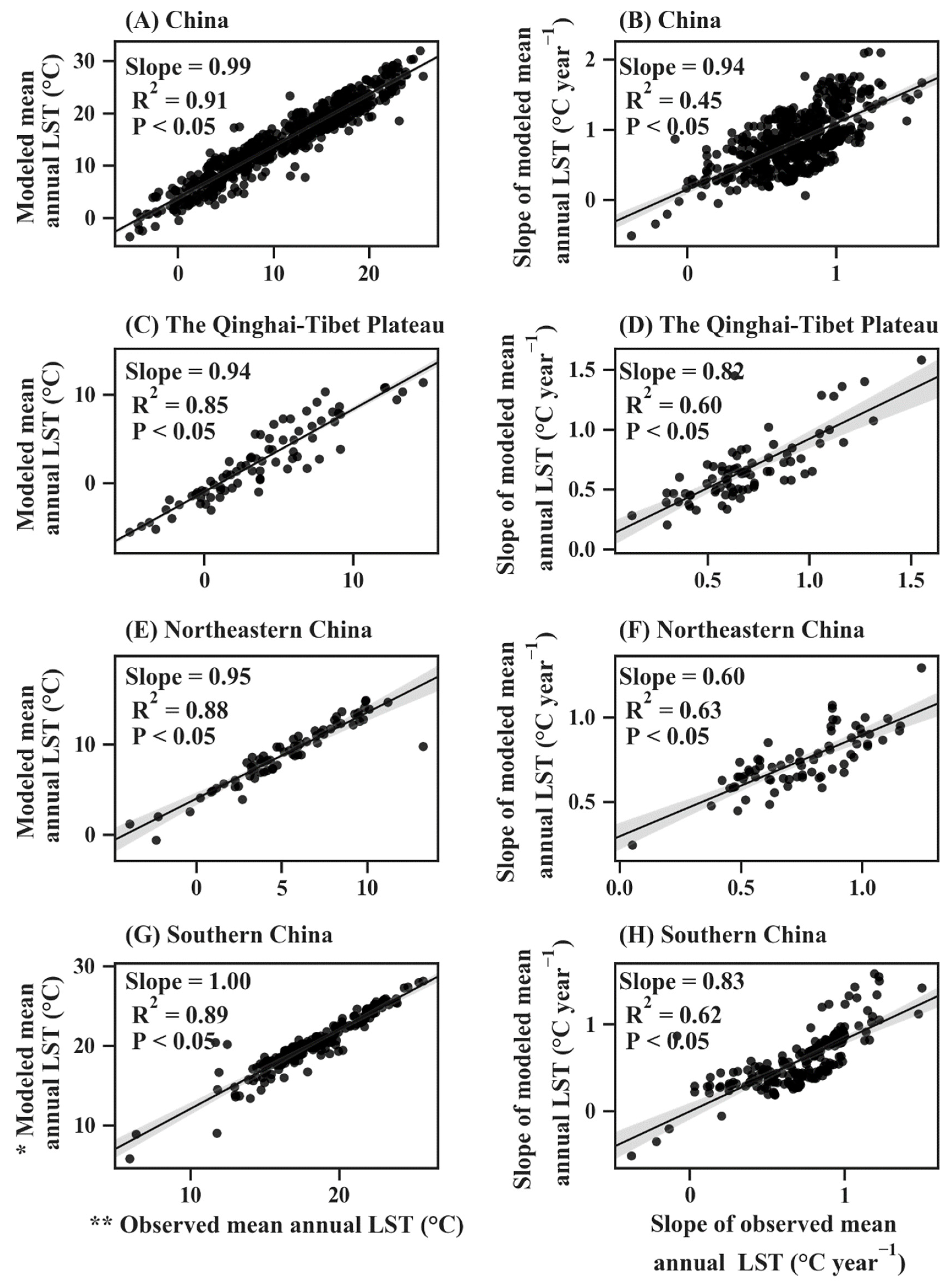
3.1. Validating LST

The mean annual LST (MAT) of 582 meteorological stations was used to validate the LST simulated by the AVHRR images. We validated the result by using the MAT from 1982 to 2016 (0). The R² of the four regions is over 0.85 (0A,C,E,G). However, the validation of the MAT trends is not as good as MAT. The value of R² is around 0.6 in the QTP, southern and northeastern China, and even lower than 0.45 in the whole of China (0B,D,F,H) but reached the significance level of 0.05. The P-value is infinitely close to 0, therefore, the specific value is not listed in Figure 2.

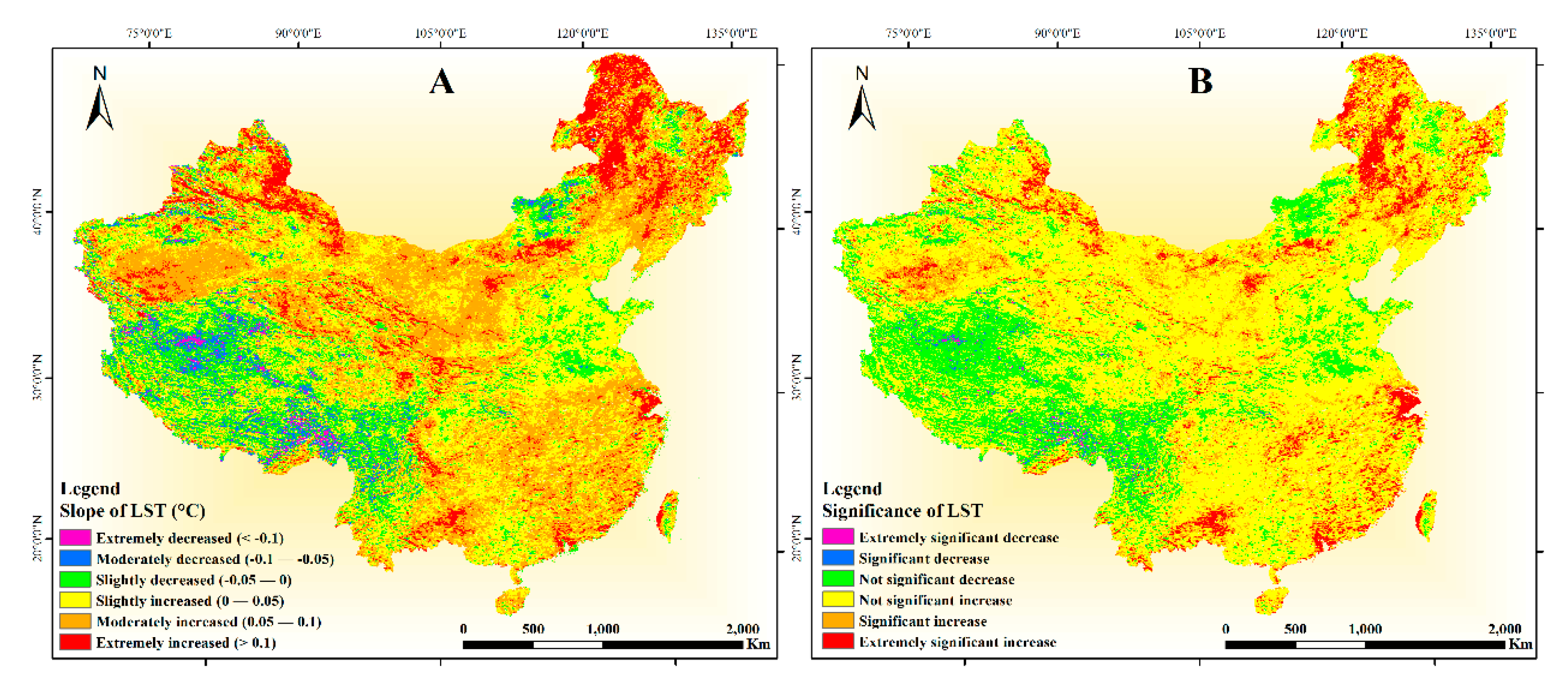
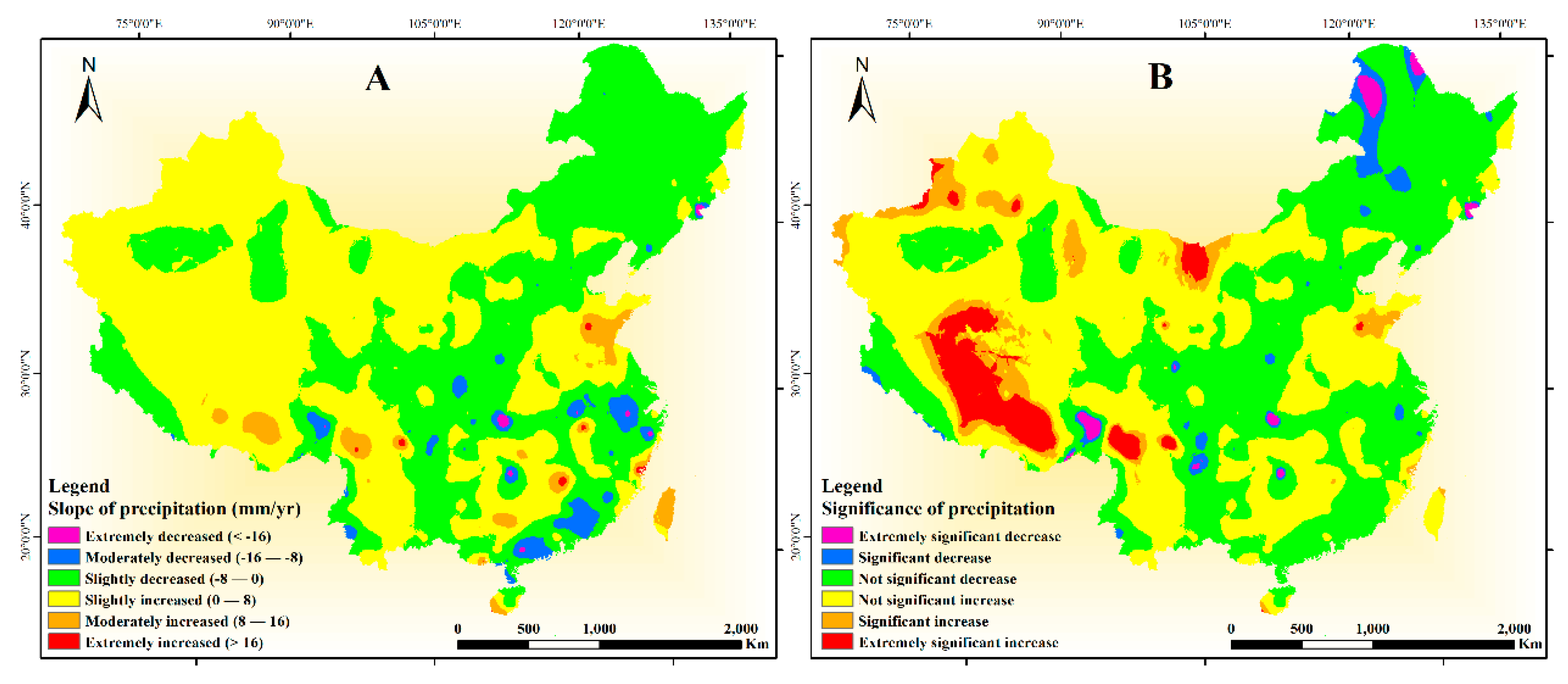
3.2. Dynamics of LST and Precipitation

Figure 3 represents a map of (A) LST trends and (B) their significance tests over China from 1982 to 2016. The identified areas that exhibited an increasing trend reached 9.5 million km², occupying 81.1% of the total land area, with an annual increase of 0.06 °C (Figure 3A). The regions that exhibited extreme and moderate increases were mainly found in northeastern and southern China, as well as in northwestern China, with areas of 4.1 and 1.3 million km², accounting for 42.8% and 13.9% of the total increased area. The regions that exhibited a slight increase accounted for an area of 4.1 million km² (43.3% of the total increased areas); such trends were scattered throughout China. Meanwhile, 2.2 million km², accounting for 9.0% of the total land area, exhibited a decreasing trend by 0.04 °C/year. Extremely and moderately decreased regions were distributed evidently in the QTP and the northeastern Inner Mongolia plateau, with areas of 0.1 million km² and 0.4 million km², occupying 4.3% and 19.8% of the total decreased area, respectively. Slightly decreased regions were mostly observed in the QTP, and a part of southwestern, eastern and northeastern China, with an area of 1.7 million km² and occupying 75.9% of the total decreased area.

The significance test is presented in Figure 3B. The area of ESI (0.8 million km²) and SI (1.5 million km²) occupied 20.0% of the total land areas; moreover, the NSI (7.2 million km²) and NSD (2.1 million km²) areas accounted for 78.9% of the total land area. Moreover, the ESD (0.05 million km²) and SD (0.07 million km²) areas accounted for only 1.1% of the total land area.

Figure 4 represents a map of (A) precipitation trends and (B) their significance tests over China from 1982 to 2016. The regions with increasing trends of precipitation accounted for 53.2% of the study areas, which were mainly found in western and southwestern China (Figure 4A). By contrast, the regions with decreasing trends of precipitation were occupying 46.7% of the study areas, which were distributed in northeastern, central China and a part of southern China. The significance test of precipitation trends is presented in Figure 4B. The ESI and SI regions were accounted for 4.7% and 5.8% of the study areas, which were mainly located in the QTP, and scattered in the northwestern and southwestern China. The ESD and SD regions were only accounted for 3.5%, which were mainly found in northeastern China.

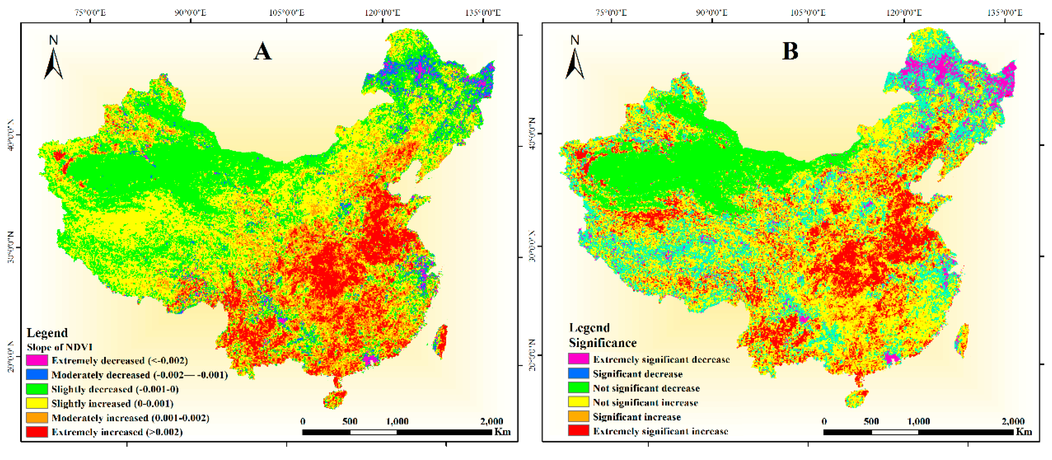
3.3. NDVI Dynamics and Significance Test

Figure 5 represents a map of (A) NDVI trends and (B) their significance tests over China from 1982 to 2016. The NDVI exhibited an increasing trend in most regions of China (Figure 5A). The identified increasing areas were 7.0 million km², occupying 58.6% of the total area. The annual average, maximum and minimum increase rate of NDVI was 0.1%, 0.01%, and 4.2%, respectively. The extremely increased regions were 0.9 million km², occupying 13.6% of the total increased area and were distributed evidently in central and eastern China. The moderately increased regions were shown a more fragmented pattern of variation; the area was 1.8 million km², accounting for 25.4% of the total increased area mainly in central and eastern China, as well as being scattered in southern China. The slightly increased regions were 4.3 million km², accounting for 35.8% of the total increased area that was widespread in China, particularly in the Qinghai–Tibet and Inner Mongolia plateaus.

By contrast, there were 4.9 million km² exhibited a decreasing rate of 0.07%/year, which was observed in northwestern and northeastern China, occupying 41.4% of the total areas. The extremely decreased regions were 0.1 million km², occupying 2.6% of the total decreased area, which was observed in the Yangtze and Pearl River deltas as well as in metropolises such as Shanghai and Guangzhou in these regions, and rapidly expanded over the past years. Moderately decreased regions were 0.5 million km², accounting for 11.0% of the total decreased area, which was mostly distributed in northeastern China. The slightly decreased regions were mainly found in northwestern China with land types characterized by desert; the area covered 4.3 million km², occupying 86.3% of the total decreased area.

According to the significance test of NDVI variation (Figure 5B), the areas of ESI (2.5 million km²) and SI (1.0 million km²) accounted for 21.1% and 8.4% of the total land areas; the areas of ESD (1.8 million km²) and SD (0.5 million km²) accounted for 15.5% and 4.2% of the total land areas, and the areas of NSI and NSD occupied 50.7% of the total land area.

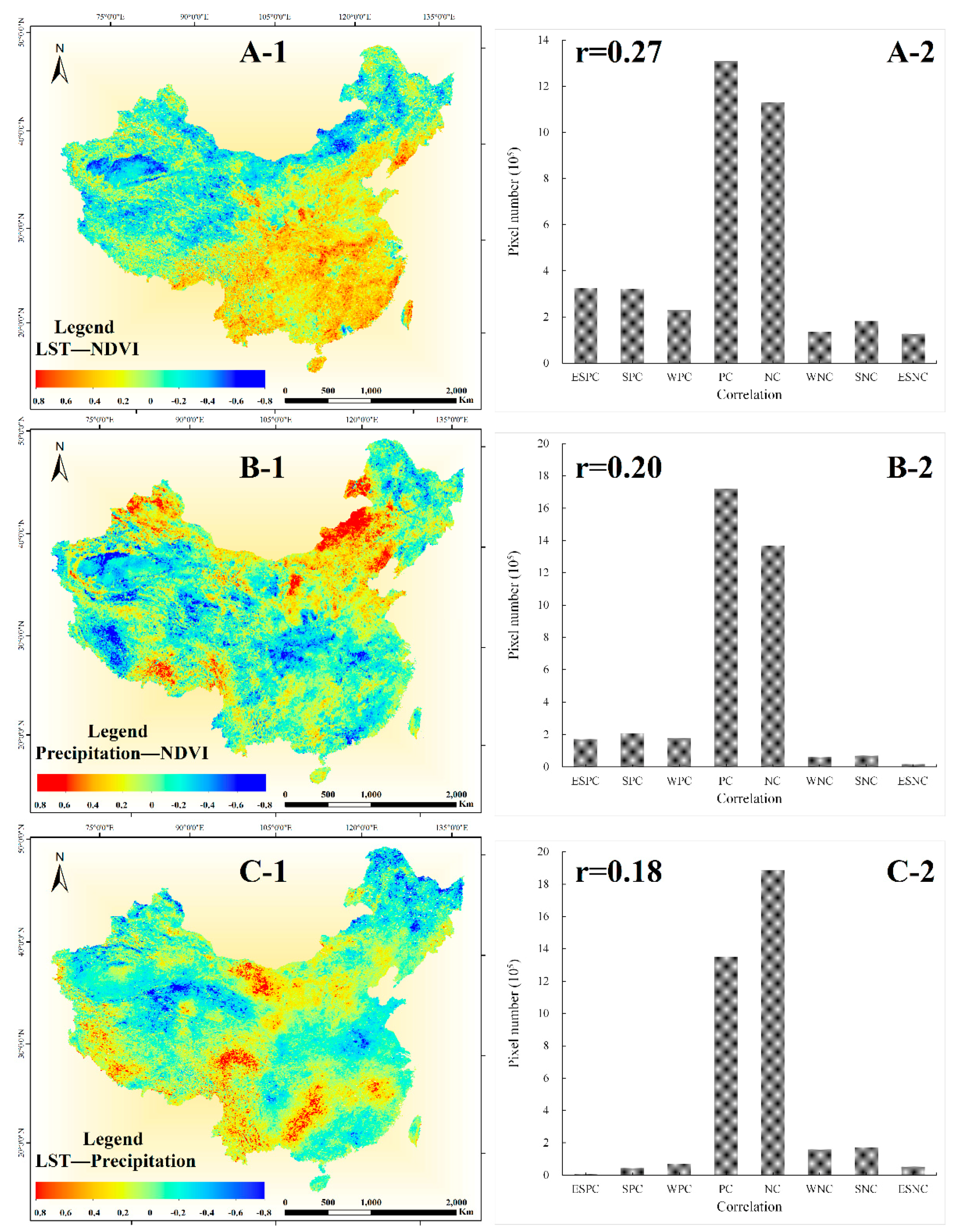
3.4. Spatiotemporal Relationship between LST and NDVI

The LST and NDVI with the highest average correlation coefficient of 0.27 (Figure 6 A-1, A-2). Positive correlation areas were mostly in southern China and occupied 57.8% of the study areas. The sum of the extremely significant (ESPC) and significant positive correlation (SPC) areas accounted for 16.9%. Only 5.7% of the study areas exhibited weak positive correlations. Positive correlation (PC) regions were up to 35.2%. By contrast, the negative correlation regions (NC) in the behavior of NDVI and LST were occupying 42.2% of the study areas. The extremely significant (ESNC), significant (SNC) and weak (WNC) negative correlation areas accounted for 2.9%, 4.7%, and 3.7% of the study areas, respectively. The average correlation coefficients between precipitation and NDVI is 0.20 (Figure 6 B-1,B-2). The regions exhibiting positive correlations were larger than those which exhibited negative correlations (60.1% vs. 39.9%). The ESPC, SPC, and WPC were occupying 4.5%, 5.5% and 4.7% of the study areas, respectively. The LST and precipitation have the lowest average correlation coefficients (r = 0.18), and not significant regularity was observed in the study areas (Figure 6 C-1,C-2). The negatively related regions accounted for 60.7% of the study areas.

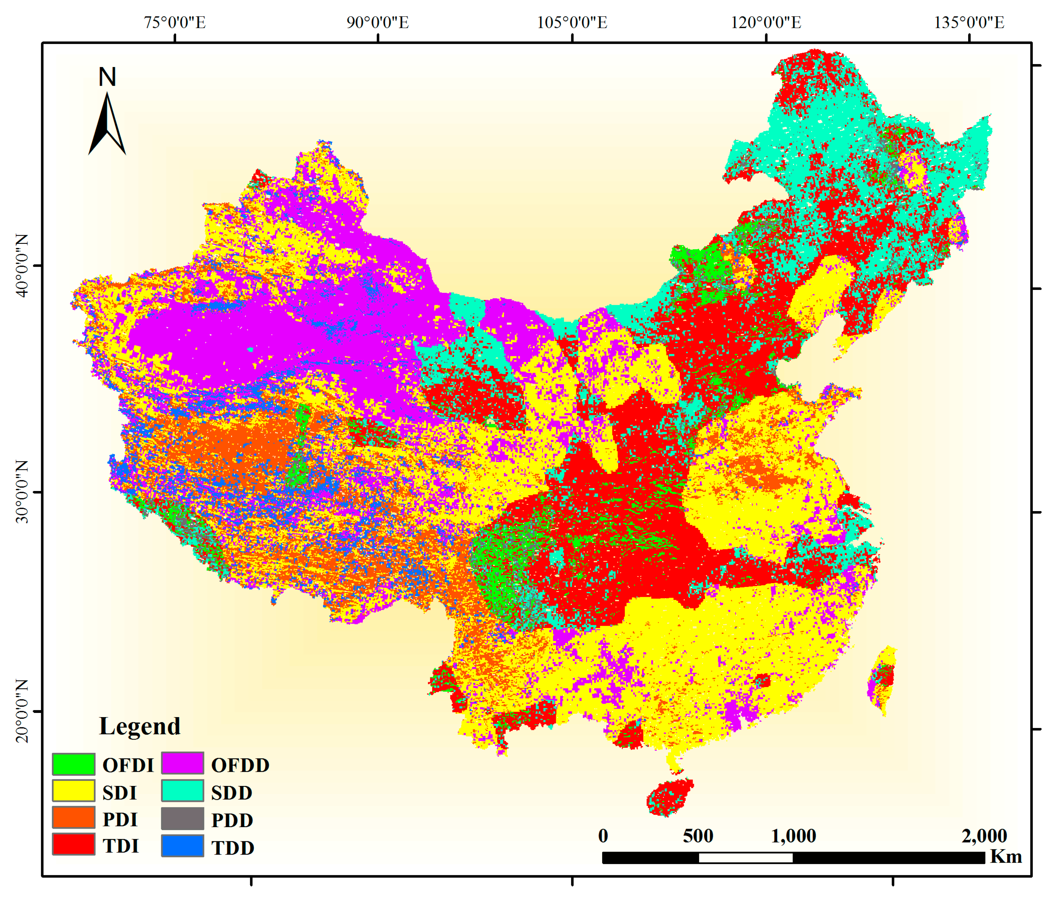
3.5. The Influencing Factors on NDVI Dynamics

The spatial distribution of the principal climate factors on vegetation dynamics is shown in Figure 7. The largest areas were the synergy of LST and precipitation dominated factors for NDVI increasing (SDI), accounting for 31.0% of the study areas, whereas the LST dominated factors for NDVI increasing (TDI) occupied 21.8% of the study areas. The precipitation factors (PDI) and other factors dominated for NDVI increasing (OFDI) only accounted for 2.0% and 3.7% of the study areas. Nearly 21.4% of the study areas were other factors dominated for NDVI decreasing (OFDD). This region mainly observed in northwestern China which characterized as the desert. In total, 14.1% of the study regions were attributed to the synergy of LST and precipitation dominated factors for NDVI decreasing (SDD), whereas the LST (TDD) and precipitation (PDD) dominated factors for NDVI decreasing occupied 4.7% and 1.3% of the study areas.

In summary, the increased LST and precipitation were the principal climate factor for NDVI increasing. It is noteworthy that decreased NDVI mainly attributed to increased LST and decreased precipitation in northeastern China.

4. Discussion

4.1. LST Retrieval Method

We detected the LST changes in China by remote sensing technology over a long study period. We found that the LST significantly increased in an environment characterized by global climate warming, with nearly 81.1% of the regions in the country experiencing an increasing trend. These regions reached significant levels, including the majority of northeastern and a part of northwestern, southeastern and southwestern China, accounting for 16.9% of the total land area; the LST increased by 0.06 °C /year. NOAA-AVHRR, as one of the suitable remote sensing images, makes it possible to monitor environmental changes over time using remote sensing. However, retrieving LST from daily to yearly data is a major challenge because of massive amounts of data and several uncertainties.

The uncertainty may be attributed to clouds and abnormal values. Although the clouds were eliminated by the QA band, erroneous cloud detection and sub-pixel clouds affected the results considerably. In this study, obtaining an entire map of the month without any missing value is different because the detected clouds mask a large part of the land surface features, especially the months from June to August. Therefore, we used a year composite method to obtain accurate data to reflect the yearly variation of LST. LSE is another uncertain factor. We employed NDVI as a basis to simulate LSE; however, the spectral behavior of natural surfaces observed from space are usually heterogeneous [48], and using NDVI causes confusion on the emissivity other than vegetation, which leads to errors in the LST simulation. Measuring the emissivity remotely is a major technical challenge that needs further study. In this study, the estimations of emissivity ranged from 0.979 to 0.99 in Channel 4 and from 0.982 to 0.99 in Channel 5.

4.2. The Scenarios and Climate Factors

This study was established eight scenarios and applied them to explore the spatial distribution of the main driving forces for the vegetation variation in China. The increase in LST certainly will benefit vegetation growth, but the extremely high-LST also could induce drought. The extreme low-LST will lead to less energy input, the effect of these conditions on vegetation might be neglect because the annual mean LST was used in the scenarios. Moreover, the annual data might ignore the seasonal mismatch in LST and precipitation.

Global warming accelerates the water cycle. The increased water vapor transports from the Arabian Sea to northwestern China because the increasing sea temperature in the South Indian Ocean enhances its water evaporation [49]. Another reason is likely due to the melting of glaciers leading to an increase in river runoff, which in turn causes an increase in precipitation [50].

Over arid regions, characterized by limited cloud cover, regional climate warming might be the main factor causing increasing LST trends. Over other regions, characterized by significant cloudiness, an increase in LST could be caused by decreasing trends in cloud cover. The NDVI was decreased significantly in northwestern China, which characterized as the desert or sparse desert vegetation. Although the precipitation was increased, however, the soil could not hold the water with the increasing temperature.

The regions with significantly decreased NDVI include northwestern and northeastern China, which matched with the findings of Xu [51], the NDVI decrease in northeastern China may be attributed to agricultural reclamation. However, this study identified increased LST and decreased precipitation in northeastern China from 1982 to 2016. Therefore, the drought-induced by LST and precipitation might be the primary cause of the decrease in NDVI in northeastern China.

4.3. The Human Activities

Human activities might be the determinant factor when climate factors to the disadvantage of the vegetation growing. Human activities like artificial irrigation, fencing enclosure, and other grassland management would benefit the growth of vegetation. The total area of the agricultural land was increased by 64.9% from 3.42 × 10⁸ ha in 1960 to 5.28 × 10⁸ ha in 2015 [52]. More importantly is that the government launched large-scale ecosystem restoration programs (e.g., the Three-North Forest Shelterbelt Program, the Grain for Green Project, and the Natural Forest Conservation Program) during the late 1990s and early 2000s, especially in northern China, to combat environmental deterioration, and forest cover has increased dramatically from 8% in 1949 to 18.2% in 2005 [53].

Human activities are also the crucial factor when city expansion (e.g., the Pearl River Delta and the Yangtze River Delta) led to decreases in NDVI. Because of human activities, an urban heat island effect is an urban area or metropolitan area that is significantly warmer than its surrounding rural areas. As the urban population in China significantly increased during this study period (1982–2016). China’s population reached 1 billion in 1982 and it reached ~1.4 billion in 2016; this led to increasing LST trends over highly-populated areas.

Overall, the effects of human activities are usually difficult to identify, which might be underestimated in vegetation degradation or restoration. Notably, northwestern and northeastern China has become more dryer because of the synergy of LST and precipitation or the desertification in vegetation decreasing. The vegetation has a positive correlation with LST in southern China, which demonstrated that increasing LST stimulates the growth of vegetation. However, whether the increase in NDVI will suppress the increase in LST remains unclear in this study and needs clear evidence to prove.

5. Conclusions

• The results of the LST simulation indicated that up to 81.1% of the total land areas exhibited with an annual increase rate of 0.06 °C/year, and 58.6% of the study areas were shown that NDVI with an average increasing rate of 0.1%/year from 1982 to 2016.
• NDVI has a higher average correlation coefficient with LST than precipitation, and the increase in LST could stimulate vegetation growth, but it is not clear that the inhibitory effect of vegetation in LST increases in this study. Northern China will become dryer because of desertification (northwestern) or climate factors (northeastern). The synergy of LST and precipitation might be the primary cause of vegetation decrease.
• The LST retrieving algorithm can be improved further. Simulating the LSE through a more precise method and improving the detection accuracy of clouds and abnormal pixels are crucial. Introducing additional parameters is also necessary to determine the discrepancy of LST in latitude and altitude.

References

- Sobrino, J.A.; Julien, Y. Trend Analysis of Global MODIS-Terra Vegetation Indices and Land Surface Temperature between 2000 and 2011. IEEE J. Sel. Top. Appl. Earth Obs. Remote Sens. 2013, 6, 2139–2145. [Google Scholar] [CrossRef]
- Zhang, R.; Tian, J.; Su, H.; Sun, X.; Chen, S.; Xia, J. Two improvements of an operational two-layer model for terrestrial surface heat flux retrieval. Sensors 2008, 8, 6165–6187. [Google Scholar] [CrossRef]
- Brunsell, N.A.; Gillies, R.R. Length scale analysis of surface energy fluxes derived from remote sensing. J. Hydrometeorol. 2003, 4, 1212–1219. [Google Scholar] [CrossRef]
- Voogt, J.A.; Oke, T.R. Thermal remote sensing of urban climates. Remote Sens. Environ. 2003, 86, 370–384. [Google Scholar] [CrossRef]
- Karnieli, A.; Agam, N.; Pinker, R.T.; Anderson, M.; Imhoff, M.L.; Gutman, G.G.; Panov, N.; Goldberg, A. Use of NDVI and Land Surface Temperature for Drought Assessment: Merits and Limitations. J. Clim. 2010, 23, 618–633. [Google Scholar] [CrossRef]
- Kustas, W.; Anderson, M. Advances in thermal infrared remote sensing for land surface modeling. Agric. For. Meteorol. 2009, 149, 2071–2081. [Google Scholar] [CrossRef]
- Wang, Z.; Gang, C.; Li, X.; Chen, Y.; Li, J. Application of a normalized difference impervious index (NDII) to extract urban impervious surface features based on Landsat TM images. Int. J. Remote Sens. 2015, 36, 1055–1069. [Google Scholar] [CrossRef]
- Townshend, J.R.G.; Justice, C.O.; Skole, D.; Malingreau, J.P.; Cihlar, J.; Teillet, P.; Sadowski, F.; Ruttenberg, S. THE 1KM RESOLUTION GLOBAL DATA SET—NEEDS OF THE INTERNATIONAL GEOSPHERE BIOSPHERE PROGRAM. Int. J. Remote Sens. 1994, 15, 3417–3441. [Google Scholar] [CrossRef]
- Sobrino, J.A.; Gómez, M.; Jiménez-Muñoz, J.C.; Olioso, A. Application of a simple algorithm to estimate daily evapotranspiration from NOAA–AVHRR images for the Iberian Peninsula. Remote Sens. Environ. 2007, 110, 139–148. [Google Scholar] [CrossRef]
- Arnfield, A.J. Two decades of urban climate research: A review of turbulence, exchanges of energy and water, and the urban heat island. Int. J. Climatol. J. R. Meteorol. Soc. 2003, 23, 1–26. [Google Scholar] [CrossRef]
- Weng, Q.H.; Fu, P. Modeling annual parameters of clear-sky land surface temperature variations and evaluating the impact of cloud cover using time series of Landsat TIR data. Remote Sens. Environ. 2014, 140, 267–278. [Google Scholar] [CrossRef]
- Sun, L.; Sun, R.; Li, X.; Liang, S.; Zhang, R. Monitoring surface soil moisture status based on remotely sensed surface temperature and vegetation index information. Agric. For. Meteorol. 2012, 166–167, 175–187. [Google Scholar] [CrossRef]
- Kerr, Y.H.; Lagouarde, J.P.; Imbernon, J. Accurate land surface temperature retrieval from AVHRR data with use of an improved split window algorithm. Remote Sens. Environ. 1992, 41, 197–209. [Google Scholar] [CrossRef]
- Sobrino, J.A.; Li, Z.-L.; Stoll, M.P.; Becker, F. Improvements in the split-window technique for land surface temperature determination. IEEE Trans. Geosci. Remote Sens. 1994, 32, 243–253. [Google Scholar] [CrossRef]
- Wan, Z.M.; Dozier, J. A generalized split-window algorithm for retrieving land-surface temperature from space. ITGRS 1996, 34, 892–905. [Google Scholar]
- Gupta, R.K.; Prasad, S.; Sai, M.; Viswanadham, T.S. The estimation of surface temperature over an agricultural area in the state of Haryana and Panjab, India, and its relationship with the Normalized Difference Vegetation Index (NDVI), using NOAA-AVHRR data. Int. J. Remote Sens. 1997, 18, 3729–3741. [Google Scholar] [CrossRef]
- Vazquez, D.P.; Reyes, F.J.O.; Arboledas, L.A. A comparative study of algorithms for estimating land surface temperature from AVHRR data. Remote Sens. Environ. 1997, 62, 215–222. [Google Scholar] [CrossRef]
- Wan, Z.M.; Zhang, Y.L.; Zhang, Q.C.; Li, Z.L. Validation of the land-surface temperature products retrieved from Terra Moderate Resolution Imaging Spectroradiometer data. Remote Sens. Environ. 2002, 83, 163–180. [Google Scholar] [CrossRef]
- Qin, Z.-h.; Karnieli, A.; Berliner, P. A mono-window algorithm for retrieving land surface temperature from Landsat TM data and its application to the Israel-Egypt border region. Int. J. Remote Sens. 2001, 22, 3719–3746. [Google Scholar] [CrossRef]
- Sobrino, J.A.; Li, Z.L.; Stoll, M.P.; Becker, F. Multi-channel and multi-angle algorithms for estimating sea and land surface temperature with ATSR data. Int. J. Remote Sens. 1996, 17, 2089–2114. [Google Scholar] [CrossRef]
- Du, C.; Ren, H.; Qin, Q.; Meng, J.; Zhao, S. A Practical Split-Window Algorithm for Estimating Land Surface Temperature from Landsat 8 Data. Remote Sens. 2015, 7, 647–665. [Google Scholar] [CrossRef] [Green Version]
- Sobrino, J.A.; Jiménez-Muñoz, J.C.; Paolini, L. Land surface temperature retrieval from LANDSAT TM 5. Remote Sens. Environ. 2004, 90, 434–440. [Google Scholar] [CrossRef]
- Cao, X.M.; Chen, X.; Bao, A.M.; Li, L.H. A study of retrieval land surface temperature and evapotranspiration based on ETM plus remote sensing data in oasis. In Proceedings of the Remote Sensing and Modeling of Ecosystems for Sustainability VII, San Diego, CA, USA, 3–4 August 2010; p. 7809. [Google Scholar] [CrossRef]
- Potter, C.; Randerson, J.T.; Field, C.B.; Matson, P.A.; Vitousek, P.M.; Mooney, H.A.; Klooster, S.A. Terrestrial ecosystem production—A process model-based on global satellite and surface data. Glob. Biogeochem. Cycles 1993, 7, 811–841. [Google Scholar] [CrossRef]
- Wang, J.; Dong, J.; Liu, J.; Huang, M.; Li, G.; Running, S.W.; Smith, W.K.; Harris, W.; Saigusa, N.; Kondo, H. Comparison of Gross Primary Productivity Derived from GIMMS NDVI3g, GIMMS, and MODIS in Southeast Asia. Remote Sens. 2014, 6, 2108–2133. [Google Scholar] [CrossRef] [Green Version]
- Zhou, W.; Li, J.L.; Mu, S.J.; Gang, C.C.; Sun, Z.G. Effects of ecological restoration-induced land-use change and improved management on grassland net primary productivity in the Shiyanghe River Basin, north-west China. Grass Forage Sci. 2014, 69, 596–610. [Google Scholar] [CrossRef]
- Wang, Z.; Zhang, Y.; Yang, Y.; Zhou, W.; Gang, C.; Zhang, Y.; Li, J.; An, R.; Wang, K.; Odeh, I.; et al. Quantitative assess the driving forces on the grassland degradation in the Qinghai–Tibet Plateau, in China. Ecol. Inform. 2016, 33, 32–44. [Google Scholar] [CrossRef]
- Wang, Z. Estimating of terrestrial carbon storage and its internal carbon exchange under equilibrium state. Ecol. Model. 2019, 401, 94–110. [Google Scholar] [CrossRef]
- Wang, Z.; Yang, Y.; Li, J.; Zhang, C.; Chen, Y.; Wang, K.; Odeh, I.; Qi, J. Simulation of terrestrial carbon equilibrium state by using a detachable carbon cycle scheme. Ecol. Indic. 2017, 75, 82–94. [Google Scholar] [CrossRef]
- Carlson, T.N.; Ripley, D.A. On the relation between NDVI, fractional vegetation cover, and leaf area index. Remote Sens. Environ. 1997, 62, 241–252. [Google Scholar] [CrossRef]
- Valor, E.; Caselles, V. Mapping land surface emissivity from NDVI: Application to European, African, and South American areas. Remote Sens. Environ. 1996, 57, 167–184. [Google Scholar] [CrossRef]
- Nemani, R.R.; Running, S.W. Estimation of Regional Surface Resistance to Evapotranspiration from NDVI and Thermal-IR AVHRR Data. J. Appl. Meteorol. 1989, 28, 276–284. [Google Scholar] [CrossRef]
- Sun, R.; Gao, X.; Liu, C.M.; Li, X.W. Evapotranspiration estimation in the Yellow River Basin, China using integrated NDVI data. Int. J. Remote Sens. 2004, 25, 2523–2534. [Google Scholar] [CrossRef]
- Johnson, L.F.; Trout, T.J. Satellite NDVI Assisted Monitoring of Vegetable Crop Evapotranspiration in California’s San Joaquin Valley. Remote Sens. 2012, 4, 439–455. [Google Scholar] [CrossRef] [Green Version]
- Hansen, M.C.; Defries, R.S.; Townshend, J.R.G.; Sohlberg, R. Global land cover classification at 1km spatial resolution using a classification tree approach. Int. J. Remote Sens. 2000, 21, 1331–1364. [Google Scholar] [CrossRef]
- Julien, Y.; Sobrino, J.A.; Mattar, C.; Ruescas, A.B.; Jimenez-Munoz, J.C.; Soria, G.; Hidalgo, V.; Atitar, M.; Franch, B.; Cuenca, J. Temporal analysis of normalized difference vegetation index (NDVI) and land surface temperature (LST) parameters to detect changes in the Iberian land cover between 1981 and 2001. Int. J. Remote Sens. 2011, 32, 2057–2068. [Google Scholar] [CrossRef]
- Julien, Y.; Sobrino, J.A. The Yearly Land Cover Dynamics (YLCD) method: An analysis of global vegetation from NDVI and LST parameters. Remote Sens. Environ. 2009, 113, 329–334. [Google Scholar] [CrossRef]
- Raynolds, M.K.; Comiso, J.C.; Walker, D.A.; Verbyla, D. Relationship between satellite-derived land surface temperatures, arctic vegetation types, and NDVI. Remote Sens. Environ. 2008, 112, 1884–1894. [Google Scholar] [CrossRef]
- Piao, S.; Mohammat, A.; Fang, J.; Cai, Q.; Feng, J. NDVI-based increase in growth of temperate grasslands and its responses to climate changes in China. Glob. Environ. Chang. Hum. Policy Dimens. 2006, 16, 340–348. [Google Scholar] [CrossRef]
- Brown, P.T.; Ming, Y.; Li, W.; Hill, S.A. Change in the magnitude and mechanisms of global temperature variability with warming. Nat. Clim. Chang. 2017, 7, 743–748. [Google Scholar] [CrossRef] [Green Version]
- Ji, F.; Wu, Z.; Huang, J.; Chassignet, E.P. Evolution of land surface air temperature trend. Nat. Clim. Chang. 2014, 4, 462–466. [Google Scholar] [CrossRef]
- Emery, W.; Camps, A. Chapter 9—Ocean Applications. In Introduction to Satellite Remote Sensing; Emery, W., Camps, A., Eds.; Elsevier: Amsterdam, The Netherlands, 2017; pp. 637–699. [Google Scholar]
- Holben, B.N. Characteristics of maximum-value composite images from temporal AVHRR data. Int. J. Remote Sens. 1986, 7, 1417–1434. [Google Scholar] [CrossRef]
- Sobrino, J.A.; Raissouni, N. Toward remote sensing methods for land cover dynamic monitoring: Application to Morocco. Int. J. Remote Sens. 2000, 21, 353–366. [Google Scholar] [CrossRef]
- Sobrino, J.A.; Jimenez-Munoz, J.C.; Soria, G.; Romaguera, M.; Guanter, L.; Moreno, J.; Plaza, A.; Martincz, P. Land surface emissivity retrieval from different VNIR and TIR sensors. IEEE Trans. Geosci. Remote Sens. 2008, 46, 316–327. [Google Scholar] [CrossRef]
- Sobrino, J.A.; Raissouni, N.; Simarro, J.; Nerry, F.; Petitcolin, F. Atmospheric water vapor content over land surfaces derived from the AVHRR data: Application to the Iberian Peninsula. IEEE Trans. Geosci. Remote Sens. 1999, 37, 1425–1434. [Google Scholar] [CrossRef]
- Kleespies, T.J.; McMillin, L.M. Retrieval of Precipitable Water from Observations in the Split Window over Varying Surface Temperatures. J. Appl. Meteorol. 1990, 29, 851–862. [Google Scholar] [CrossRef] [Green Version]
- Li, Z.L.; Wu, H.; Wang, N.; Qiu, S.; Sobrino, J.A.; Wan, Z.M.; Tang, B.H.; Yan, G.J. Land surface emissivity retrieval from satellite data. Int. J. Remote Sens. 2013, 34, 3084–3127. [Google Scholar] [CrossRef]
- Shi, Y.; Shen, Y.; Li, D.; Zhang, G.; Ding, Y.; Hu, R.; Kang, E. Discussion on the present climate change from warm-dry to warm-wet in Northwest China. Quat. Sci. 2003, 23, 152–164. [Google Scholar]
- Wang, Z.; Chang, J.; Peng, S.; Piao, S.; Ciais, P.; Betts, R. Changes in productivity and carbon storage of grasslands in China under future global warming scenarios of 1.5 °C and 2 °C. J. Plant Ecol. 2019, 12, 804–814. [Google Scholar] [CrossRef]
- Xu, G.; Zhang, H.; Chen, B.; Zhang, H.; Innes, J.; Wang, G.; Yan, J.; Zheng, Y.; Zhu, Z.; Myneni, R. Changes in Vegetation Growth Dynamics and Relations with Climate over China’s Landmass from 1982 to 2011. Remote Sens. 2014, 6, 3263–3283. [Google Scholar] [CrossRef] [Green Version]
- Lee, K.S.; Lee, D.S.; Min, S.W.; Kim, S.C.; Seo, I.-H.; Chung, D.Y. Spatial changes and land use of arable land in China. Korean J. Soil Sci. Fertil. 2018, 51, 327–338. [Google Scholar]
- Cao, S.; Chen, L.; Shankman, D.; Wang, C.; Wang, X.; Zhang, H. Excessive reliance on afforestation in China’s arid and semi-arid regions: Lessons in ecological restoration. Earth-Sci. Rev. 2011, 104, 240–245. [Google Scholar] [CrossRef]