The Bike-Sharing Rebalancing Problem Considering Multi-Energy Mixed Fleets and Traffic Restrictions

Abstract

Nowadays, as a low-carbon and sustainable transport mode bike-sharing systems are increasingly popular all over the world, as they can reduce road congestion and decrease greenhouse gas emissions. Aiming at the problem of the mismatch of bike supply and user demand, the operators have to transfer bikes from surplus stations to deficiency stations to redistribute them among stations by vehicles. In this paper, we consider a mixed fleet of electric vehicles and internal combustion vehicles as well as the traffic restrictions to the traditional vehicles in some metropolises. The mixed integer programming model is firstly established with the objective of minimizing the total rebalancing cost of the mixed fleet. Then, a simulated annealing algorithm enhanced with variable neighborhood structures is designed and applied to a set of randomly generated test instances. The computational results and sensitivity analysis indicate that the proposed algorithm can effectively reduce the total cost of rebalancing.

1. Introduction

Nowadays, bike-sharing systems (BSSs), as a low-carbon and sustainable transport mode, are becoming more and more popular across the global, as they can reduce road congestion and decrease greenhouse gas emissions caused by motorized transportation [1,2]. The first BSS was introduced in Amsterdam in 1965 [3] and there are now more than 1500 active BSSs [4] and this number is growing at an increasing rate [5,6]. Recently, some scholars begin to pay attention to the practical problem of mismatch of bike supply and user demands in the BSS, which is a common challenge to all BSS operators [7]. Some operators are trying to meet user demand by placing bikes in cities in large numbers, but this creates congestion on city streets and is not sustainable. In China, the government has introduced policies to restrict operators from placing too many bikes. Thus, these operators have to transfer bikes from the surplus stations to the deficiency stations by means of vehicles so that the BSS can be rebalanced. This problem is known as the Bike-sharing Rebalancing Problem (BRP) [8].

Originally, the BSS operators employ internal combustion vehicles (ICVs) to do the rebalancing operations. However, the development of electric vehicles (EVs) has made great progress over the past few years and many BSS operators are discovering that EVs bring more advantages than ICVs beyond environmental benefits, such as less maintenance, less noise pollution and reduced driving cost [9]. The Chinese government has strongly supported companies to develop sustainable EVs in recent years, providing many policy bonuses for the purchase and use of EVs. Furthermore, more and more cities have implemented traffic restrictions on ICVs to reduce carbon emissions and alleviate traffic congestions [10]. In these cities, ICVs cannot provide services for certain BSS stations in the restricted areas, while EVs can. Therefore, in many practical situations, a multi-energy mixed fleet, consisting of both EVs and ICVs, are used to perform the rebalancing operations.

In this study, the original version of the BRP is extended by assuming the fleet of vehicles to be multi-energy types. The BRP considering Multi-energy Mixed Fleets and Traffic Restrictions (BRP-MMFTR) is considered to be an NP-hard problem, for it originates from the classical Vehicle Routing Problem (VRP). We formulate the BRP-MMFTR as a mixed integer programming model based on one commodity pickup and delivery problem [11], with the objective of minimizing the total rebalancing cost of the mixed fleet. Our model has more complicate constraints than general BRP, such as battery capacity limits for EVs and traffic restrictions for ICVs. It is therefore more complex and more difficult to solve. As the size of bike-sharing stations increases, the calculation time will increase exponentially. Hence, the real-life BRP-MMFTR instances cannot be solved exactly within acceptable computation time.

To handle BRP-MMFTR in a runtime acceptable to BSS operators, we propose the Simulated Annealing algorithm with Variable Neighborhood structures (SAVN) to obtain the optimal solution. To avoid getting into the trap of local optima and enhance the exploratory capability, several variable neighborhood structures are incorporated in our algorithm.

The contribution of this paper lies on the following:

• To introduce a new and practical bike-sharing rebalancing problem considering multi-energy mixed fleets and traffic restrictions;
• To present a mixed integer programming model to formulate the problem above;
• To propose a simulated annealing algorithm with several variable neighborhood structures to solve it.

The remainder of this paper is organized as follows. Section 2 presents the literature review on the related problems. Section 3 formally presents a mixed integer programming formulation for BRP-MMFTR. Section 4 describes the procedure and key components of SAVN. Section 5 contains the computational experiments and a sensitivity analysis. Finally, Section 6 presents some concluding remarks about this work.

2. Literature Review

The BRP has been receiving considerable attention from the literatures during the past decade. Most of studies have focused on optimization models that maximize profits or minimize costs. Dell’ Amico et al. provide four mixed integer programming models with the objective of minimizing total costs, where a fleet of capacitated vehicles is employed to relocate the bikes [12]. Erdoğan et al. and Cruz et al. solve the same model proposed by Dell’ Amico with a single vehicle, where multi-visit strategy is considered at each station [11,13]. Duan et al. focus on multi-vehicle BRP with the objective of minimizing the total travel distance, and a greedy algorithm is proposed [14]. Casazza et al. and Bulhões et al. incorporate time into the constraints such that each route does not exceed service time limitation [5,15].

All the problems above need to fully meet the rebalancing demands in the BSS, which is difficult to achieve in reality. Hence, some researchers are trying to relax these constraints, and setting the objective to maximize the satisfied rebalancing demand. Papazek et al. set the primary goal to minimize the absolute deviation between target and final fill levels for all stations [16]. Gaspero et al. solve the problem with the aim of minimizing the weighted sum of the total travel time and the total absolute deviation from the target number of bikes [17], while Raviv and Kolka take it as a penalty cost [18]. Faulty bikes are considered by Wang and Szeto with the objective of minimizing the total carbon emission of all vehicles [19]. Usama et al. also consider replacing faulty bikes in the system with the following objectives: user dissatisfaction and vehicle routing costs [20].

Actually, BRP is a large-scale uncertainty problem, due to the existence of uncertainty of user demand [21]. Hence, some scholars have turned their attention to the BRP with uncertain user demand. There are roughly three types of methods for dealing with these uncertainty problems. First, prediction is a common method to resolve uncertainty. Alvarez-Valdes et al. estimate the unsatisfied demand to guide rebalancing algorithms [3]. Zhang et al. propose a dynamic bike rebalancing method that considers both bike rebalancing, vehicle routing and the prediction of inventory level and user arrivals [22]. Second, some scholars divide the uncertainty into multiple independent stochastic scenarios for research. Dell’Amico et al. develop the stochastic programming model with the objective of minimizing the travel cost and the penalty costs for unfulfilled demands [23]. Maggioni et al. propose the two-stage and multi-stage stochastic optimization models to determine the optimal number of bikes to assign to each station [24]. Yuan et al. present a mixed integer programming model with the objective of minimizing the daily costs including the capital cost and the expected operating cost [25]. Third, some studies deal uncertainty directly with dynamic factors. Legros focuses on dynamic rebalancing strategy in the BSS with the objective of minimizing the rate of arrival of unsatisfied users, and solve it by a Markov decision process approach [26]. You develops a constrained mathematical model to deal with a multi-vehicle BRP, aiming to develop dynamic decisions to minimize the sum of the travel costs and unmet costs under service level constraints over a planning horizon [27].

However, none of these literature works considers multi-energy mixed fleets. Goncalves et al. consider the vehicle routing problem with pickup and delivery, and propose a heterogeneous vehicle routing model based on ICVs and EVs [28]. Sassi et al. formulate the heterogeneous electric vehicle routing problem with time dependent charging costs, in which a set of customers have to be served by a mixed fleet of vehicles composed of ICVs and EVs [29]. A mixed fleet of ICVs and EVs are also considered in Goeke and Schneider [30]. The authors formulate the electric vehicle routing problem with time windows and mixed fleet, which is solved through adaptive large neighborhood search algorithm. Charging times vary according to the battery level when the EV arrives at the charging station, and charging is always done up to maximum battery capacity. Macrina et al. present a new variant of the green vehicle routing problem with time windows and propose an iterative local search heuristic to optimize the routing of a mixed vehicle fleet, composed of EVs and ICVs [31].

In summary, there are abundant studies about BSS, but no model considers multi-energy mixed fleets and traffic restrictions. For real-life BSSs in big cities, it is more realistic and more useful to consider a fleet of EVs and ICVs. Therefore, in this paper, we focus on a new and practical variant of BRP under the background of multi-energy mixed fleets (composed of EVs and ICVs) and traffic restrictions to ICVs. Our contribution to the development and application of the BSS model is twofold. On the one hand, we formulate BRP-MMFTR as a mixed integer programming model with the objective of minimizing the total rebalancing cost. On the other hand, because this model is too complex to be solved accurately, we develop SAVN to solve it. Our work will expand the existing knowledge on modeling BSS.

3. Model Formulation

3.1. Model Descripion and Notations

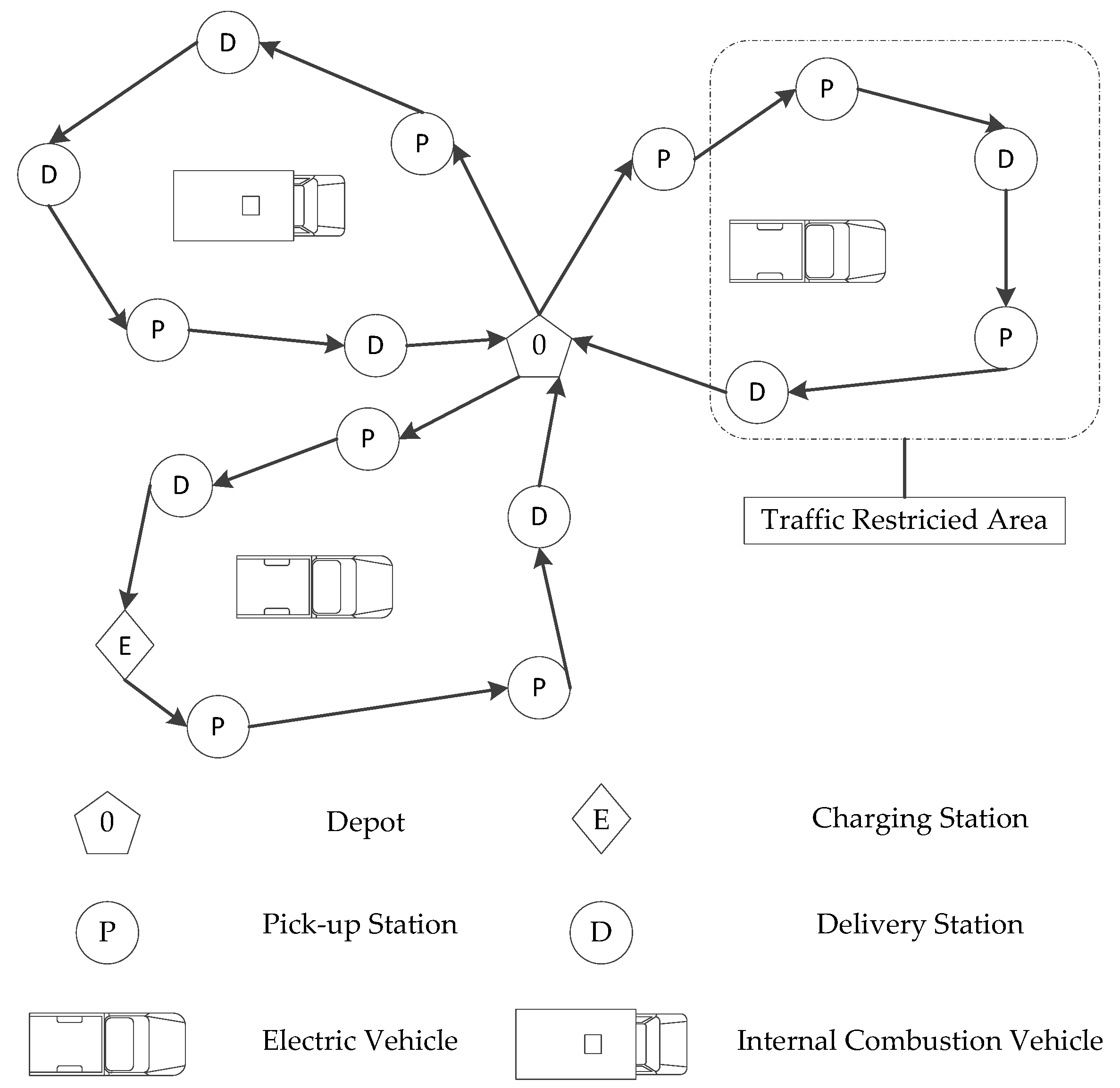
As shown in Figure 1, BRP-MMFTR studied in this paper can be described as follows: There are two types of vehicles available, namely EVs and ICVs. Vehicles start from the depot with no inventory of bikes, then serve all stations by sequentially loading excess bikes or unloading insufficient bikes, and finally return to the depot after serving all stations. Each station can be served by a vehicle only once. During the rebalancing process, the number of bikes carried by a vehicle cannot exceed its maximal capacity. EVs need to visit the charging stations during the service process. To reduce the complexity of our model, the EV battery must be fully charged at any charging station and the depot. In addition, ICVs are not allowed to enter the traffic restricted area. The objective of BRP-MMFTR is to minimize the total rebalancing cost including the vehicles’ fixed costs and traveling energy costs, recharging costs for EVs, and carbon emissions for ICVs.

The assumptions related to BRP-MMFTR are given as follows:

• All stations’ demands are known and fixed;
• The traveling energy costs and carbon emissions are only related to the travel distances;
• The loading and unloading time are neglected;
• The residual charge level of the EV grows linearly with the charging time;
• All homogeneous vehicles run at a uniform speed;
• The number of vehicles in the depot and the number of charging piles in each charging stations are sufficient;

The notations of sets, parameters, and decision variables used in our model are listed in

Table 1. Description of notations.

Sets	Description
0	The depot.
$\mathit{N}$	The set of stations, $\mathit{N} = \{1, 2, \dots , \mathit{n}\}$.
$\mathit{A}$	The set of arcs, $\mathit{A} = \left\{\right(\mathit{i}, \mathit{j})/\mathit{i}, \mathit{j} \in \mathit{N} \cup \left\{0\right\}, \mathit{i} \ne \mathit{j}\}$.
$\mathit{E}$	The set of charging stations, $\mathit{E}= \{1,2, \dots , \mathit{e}\}$.
${\mathit{K}}_1$	The set of ICVs, ${ \mathit{K}}_{1 }{= \{1,2, \dots , \mathit{k}}_1\}$.
${\mathit{K}}_2$	The set of EVs,${ \mathit{K}}_2{ = \{\mathit{k}}_1{ + 1, \mathit{k}}_1{ + 2, \dots , \mathit{k}}_2\}$.
$\mathit{K}$	The set of vehicles, ${\mathit{K}=\mathit{K}}_1\cup {\mathit{K}}_2$.
$\mathit{S}$	The set of auxiliary variables avoiding sub-loops, $\mathit{S}\subseteq \mathit{N}$.
$\mathit{D}$	The set of stations in restricted area,$\mathit{D}\subseteq \mathit{N}$.
Parameters	Description
${\mathit{Q}}^{\mathit{k}}$	The maximal capacity of vehicle $\mathit{k}$.
${\mathit{F}}^{\mathit{k}}$	The fixed cost of vehicle $\mathit{k}$.
${\mathit{C}}_{\mathit{ij}}^{\mathit{k}}$	The unit energy cost from vertex $\mathit{i}$ to vertex $\mathit{j}$ of vehicle $\mathit{k}$.
${\mathit{d}}_{\mathit{ij}}$	The distance from vertex $\mathit{i}$ to vertex $\mathit{j}$.
${R}$	The maximum battery level of EVs.
${\mathit{u}}_{\mathit{ik}}^1$	The residual charge of EV $\mathit{k}$ when reaching vertex $\mathit{i}$.
${\mathit{u}}_{\mathit{ik}}^2$	The residual charge of EV $\mathit{k}$ when leaving vertex $\mathit{i}$.
$\mathit{\lambda }$	The unit charging rate of EV.
$\mathit{r}$	The unit battery energy consumption of EV.
$\mathit{\mu }$	The coefficient of safe-residual-charge level of EV.
${\mathit{t}}_{\mathit{e}}^{\mathit{k}}$	The charging time of EV $\mathit{k}$ at charging station $\mathit{e}$.
${\mathit{C}}_{\mathit{w}}$	The unit cost of charging time.
$\mathit{L}$	The unit carbon emission of ICV.
${\mathit{C}}_{\mathit{L}}$	The unit carbon trade cost.
${\mathit{G}}_{\mathit{i}}$	The bike demand at station $\mathit{i}$.
${\mathit{g}}_{\mathit{ij}}^{\mathit{k}}$	The number of bikes loaded when vehicle $\mathit{k}$ is on arc $(\mathit{i}, \mathit{j})$.
Decision variables	Description
${\mathit{x}}_{\mathit{ij}}^{\mathit{k}}$	Binary variable, 1 if vehicle $\mathit{k}$ traverses arc $(\mathit{i}, \mathit{j})$, and 0, otherwise.
${\mathit{y}}_{\mathit{e}}^{\mathit{k}}$	Binary variable, 1 if vehicle $\mathit{k}$ is charged at charging station $e$, and 0, otherwise.

.

3.2. The Total Rebalancing Cost

The total rebalancing cost of BRP-MMFTR include four parts: vehicles’ fixed costs, vehicles’ traveling energy costs, EV recharging costs, and ICVs’ carbon emission costs. The vehicles’ fixed costs and traveling energy costs are the basic components of objectives in most traditional VRP models. In the objective of our model, the recharging costs reflect the additional charging time during the operation of EVs, while the carbon emission costs are related to the greenhouse gas emission of ICVs.

(1) Fixed costs (${\mathrm{C}}_1$)

The fixed costs of vehicles are the costs of using vehicles for rebalancing operations. They are different for EVs and ICVs, and the equation of vehicles’ fixed costs in our model is shown as follows:

$$C_1={\displaystyle \sum }_{k\in K}{\displaystyle \sum }_{j\in N, j\ne 0}{x}_{0j}^k\cdot F^k$$

(1)

(2) Traveling energy costs (${\mathrm{C}}_2$)

The traveling energy costs are composed of two types of costs, that is, fuel costs of ICVs and electricity costs of EVs. Both of them are only associated with the travel distance. And the equation of vehicles’ traveling energy costs is shown as follows:

$$C_2={\displaystyle \sum }_{k\in K}{\displaystyle \sum }_{\left(i,j\right)\in A,i\ne j}{C}_{ij}^k \cdot { d}_{ij }\cdot { x}_{ij}^k$$

(2)

(3) Recharging costs (${\mathrm{C}}_3$)

The travel distance of an EV is limited by its maximum battery level. Hence, it needs to be charged when its residual charge level lower than the safe residual charge level. The recharging cost is only related to the charging time. The equation of recharging costs is shown as follows:

$$C_3={\displaystyle \sum }_{k\in K_2}{\displaystyle \sum }_{e\in E}{C}_w\cdot t_e^k\cdot y_e^k$$

(3)

(4) Carbon emission costs (${\mathrm{C}}_4$)

In the process of rebalancing, a large amount of CO₂ is generated by ICVs from their fuel consumptions, resulting in greenhouse effect. By reducing the costs of carbon emissions, the total rebalancing cost is reduced. The equation of carbon emission costs is shown as follows:

$$C_4={\displaystyle \sum }_{k\in K_1}{\displaystyle \sum }_{\left(i,j\right)\in A,i\ne j}L\cdot C_L\cdot d_{ij}\cdot x_{ij}^k$$

(4)

3.3. Model Establishment

The mixed integer programming model for BRP-MMFTR can be written as follows:

$$\begin{gathered} min\hspace{1em}Z=C_1 + C_2 + C_3 + C_4={\displaystyle \sum }_{k\in K}{\displaystyle \sum }_{j\in N,j\ne 0}{x}_{0j}^k\cdot F^k+{\displaystyle \sum }_{k\in K}{\displaystyle \sum }_{\left(i,j\right)\in A,i\ne j}{C}_{ij}^k \cdot d_{ij} \cdot x_{ij}^k \\ +{\displaystyle \sum }_{k\in K_2}{\displaystyle \sum }_{e\in E}{C}_w\cdot t_e^k\cdot y_e^k+{\displaystyle \sum }_{k\in K_1}{\displaystyle \sum }_{\left(i,j\right)\in A,i\ne j}L\cdot C_L\cdot d_{ij}\cdot x_{ij}^k \end{gathered}$$

(5)

Subject to:

$${\displaystyle \sum }_{j\in N,j\ne 0}{x}_{0j}^k={\displaystyle \sum }_{i\in N,i\ne 0}{x}_{i0}^k=1 \hspace{1em}\forall k \in K$$

(6)

$${\displaystyle \sum }_{k\in K}{\displaystyle \sum }_{j\in N,j\ne i}{x}_{ij}^k=1 \hspace{1em}\forall i \in N$$

(7)

$${\displaystyle \sum }_{j\in N,j\ne i}{x}_{ij}^k-{\displaystyle \sum }_{j\in N,j\ne i}{x}_{ji}^k=0 \hspace{1em}\forall i \in N,\forall k \in K$$

(8)

$${\displaystyle \sum }_{i\in S}{\displaystyle \sum }_{j\in S}{x}_{ij}^k\le \left|S\right| - 1 \hspace{1em}\forall S \subseteq N, \left|S\right|\ge 2$$

(9)

$${\displaystyle \sum }_{j\in D,j\ne i}{x}_{ij}^k=0 \hspace{1em}\forall i \in N,\forall j \in D,\forall k \in K_1$$

(10)

$$max\left\{0,G_i,G_j\right\} \cdot x_{ij}^k \le g_{ij}^{k }\le min\left\{Q^k,Q^k + G_i,Q^k-G_j\right\} \cdot x_{ij}^k\hspace{1em}\forall i,j \in N, i\ne j$$

(11)

$${\displaystyle \sum }_{k\in K}{\displaystyle \sum }_{j\in N,j\ne i}{g}_{ij}^k-{\displaystyle \sum }_{k\in K}{\displaystyle \sum }_{j\in N,j\ne i}{g}_{ji}^k=G_i\hspace{1em}\forall i\in N$$

(12)

$$0\le g_{ij}^k \le Q^k\cdot x_{ij}^k\hspace{1em}\forall i,j\in N, i\ne j, \forall k \in K$$

(13)

$$t_e^k=y_e^k\cdot \left[\left(R-u_{ek}^1\right)/\lambda \right]\hspace{1em}\forall k \in K_2,\forall e \in E$$

(14)

$$0 \le { u}_{jk}^1 \le u_{ik}^2-r\cdot d_{ij}\cdot x_{ij}^k+R \cdot \left(1-x_{ij}^k\right)\hspace{1em}\forall i,j \in N, i\ne j,\forall k \in K_2$$

(15)

$$u_{ik}^1\ge \mu \cdot R \hspace{1em}\forall i \in N, \forall k \in K_2$$

(16)

$$u_{0k}^2=R \hspace{1em}\forall k \in K_2$$

(17)

$$u_{ek}^2=y_e^k\cdot R \hspace{1em}\forall k \in K_2,\forall e \in E$$

(18)

$$u_{ik}^1=u_{ik}^2\hspace{1em}\forall i \in N,\forall k \in K_2$$

(19)

$$x_{ij}^k, y_e^k = \left[0,1\right]\hspace{1em}\forall i \in N,\forall j \in N,\forall k \in K,\forall e \in E$$

(20)

Objective function (5) minimizes the total rebalancing cost, including vehicles’ fixed costs, vehicles’ traveling energy costs, EVs’ recharging costs, and ICVs’ carbon emission costs. Constraints (6) ensure that each vehicle starts at the depot and returns to the depot at the end of its route. Constraints (7) guarantee that each station is served exactly once. Constraints (8) refer to the usual flow conservation. Constraints (9) can avoid subtours and thus guarantee route-connectivity. Constraints (10) indicate that ICVs are restricted from entering the restricted area. Constraints (11) give the upper and lower bounds of the number of bikes loaded by vehicles. Constraints (12) and (13) ensure that the vehicle’s maximum capacity is not exceeded. Constraints (14) and (15) are the EVs’ charging functions and power consumption functions, respectively. Constraints (16) indicate the safe residual charge constraints of EVs. Constraints (17) and (18) show that EVs are fully charged when leaving the depot or a charging station. Constraints (19) guarantee the residual charges of EVs are the same after serving a BSS station. Constraints (20) are the binary decision variables.

4. Simulated Annealing Algorithm with Variable Neighborhood Structures

Simulated Annealing (SA) is a heuristic method to solve various NP-hard optimization problems. It can expand the exploration capability by accepting worsen solutions with some probability. This has benefit to reduce the probability of getting trapped in local optima. In order to improve the search efficiency and get solutions with higher quality, we introduce the variable neighborhood structures [32] into the framework of SA, and propose SAVN to deal with the real-life BRP-MMFTR instances. The procedure and key components of our algorithm are described in detail below.

4.1. The Procedure of Our Algorithm

Given an initial solution, SAVN starts from the initial temperature ${\mathit{T}}_0$. During the search process, the algorithm randomly selects a neighborhood structure to transform the current solution S into a randomly generated feasible neighbor ${\mathit{S}}^{\prime }$. Note that the cost of a feasible solution S, namely $\mathit{Z}\left(\mathit{S}\right)$, is evaluated with the Equation (5). If the cost of ${\mathit{S}}^{\prime }$ is less than the cost of S, ${\mathit{S}}^{\prime }$ will definitely be accepted. Otherwise, the acceptance probability of ${\mathit{S}}^{\prime }$ is $\mathit{p} = \mathit{e}\mathit{x}\mathit{p}\left(-\frac{\mathit{Z}\left({\mathit{S}}^{\prime }\right)-\mathit{Z}\left(\mathit{S}\right)}{\mathit{T}}\right)$, where T is the current temperature. For each T, this process is performed $\mathit{L}\mathit{e}\mathit{n}$ times. Then, T decreases by multiplying the cooling rate $\mathit{\alpha }$.

Repeating the above processes until the stop criterion is met, that is, the unimproved number of the best solution so far reaches the pre-specified MaxUN. Furthermore, when T is less than 0.01, T will increase to help the algorithm escape from the local optima [33]. We double ${\mathit{T}}_{\mathit{b}}$ first (but no more than ${\mathit{T}}_0$) and then set ${\mathit{T} = \mathit{T}}_{\mathit{b}}$. The pseudocode of SAVN is shown in Algorithm 1.

Algorithm 1 The procedure of SAVN
1	Parameters:${\mathit{S}}^{*}$ (the best solution so far), ${\mathit{T}}_0$ (the initial temperature), ${\mathit{T}}_b$ (the temperature with which ${\mathit{S}}^{*}$ is found), MaxUN (the maximum unimproved number of the best solution), $Len$ (maximum number of iterations at the current temperature), ${\mathit{N}}_{\mathit{k}}$ (the neighborhood structures, $\mathit{k} = 1,\cdots ,{\mathit{k}}_{\mathit{m}\mathit{a}\mathit{x}}$), $\mathit{\alpha }$ (the cooling rate)
2	Construct S as an initial solution
3	${\mathit{S}}^{*} = \mathit{S}$, $\mathit{T} = {\mathit{T}}_0$, ${\mathit{T}}_{\mathit{b}} = {\mathit{T}}_0$, count = 0
4	while count < MaxUN
5	for $\mathit{n} = 1$ to $\mathit{Len}$
6	Select randomly a neighborhood structure ${\mathit{N}}_{\mathit{k}}$
7	Generate a feasible solution ${\mathit{S}}^{\prime }$ from $\mathit{S}$ with ${\mathit{N}}_{\mathit{k}}$
8	if $\mathit{Z}\left({\mathit{S}}^{\prime }\right) < \mathit{Z}\left(\mathit{S}\right)$
9	$\mathit{S} = {\mathit{S}}^{\prime }$
10	else
11	Set $\mathit{S} = {\mathit{S}}^{\prime }$ with probability $p = exp\left(-\frac{Z\left(S^{\prime }\right)-Z\left(S\right)}{T}\right)$
12	end
13	if $Z\left(S\right) < Z\left(S^{*}\right)$
14	${\mathit{S}}^{*} = S$, $T_b = \mathit{T}$, count = 0
15	else
16	count = count + 1
17	end
18	end
19	$T = \alpha *T$
20	if$\mathit{T} < 0.01$
21	$T_b=\min \{2*T_b, {\mathit{T}}_0\}$, ${\mathit{T}=\mathit{T}}_{\mathit{b}}$
22	end
23	end
24	Return${\mathit{S}}^{*}$

4.2. Initial Solution Generation

Considering the particularity of BRP-MMFTR, we firstly classify all BSS stations into two types by region: stations in restricted areas and stations in non-restricted areas. Then a three-step algorithm is proposed to generate the high-quality initial solution.

Step 1: For stations in the restricted areas, EVs must be employed. We use the insert algorithm to construct the initial routes for these stations. First, the station with the largest distance from the depot is selected as the first customer of an EV. Then, if the capacity constraints are satisfied, the other stations are inserted into the current EV route in turn. Otherwise, a new EV route will be generated and serve the remainder stations. Repeat this insertion process until all stations in the restricted areas are serviced.

Step 2: For the stations in non-restricted areas, we first judge whether a station can be inserted into the existing EV routes. For the stations that can be inserted, we insert them to the positions with the lowest incremental cost in the existing EV routes. For the other stations, we employ the same insert algorithm to generate some new ICV routes.

Step 3: Charging stations are allocated to EV routes. If the residual charge level of an EV is enough, this step can be skipped. Otherwise, when the residual charge level of an EV is lower than the designated safe-residual-charge level, the nearest charging station will be inserted into the EV route to increase its mileage.

4.3. Neighborhood Structures

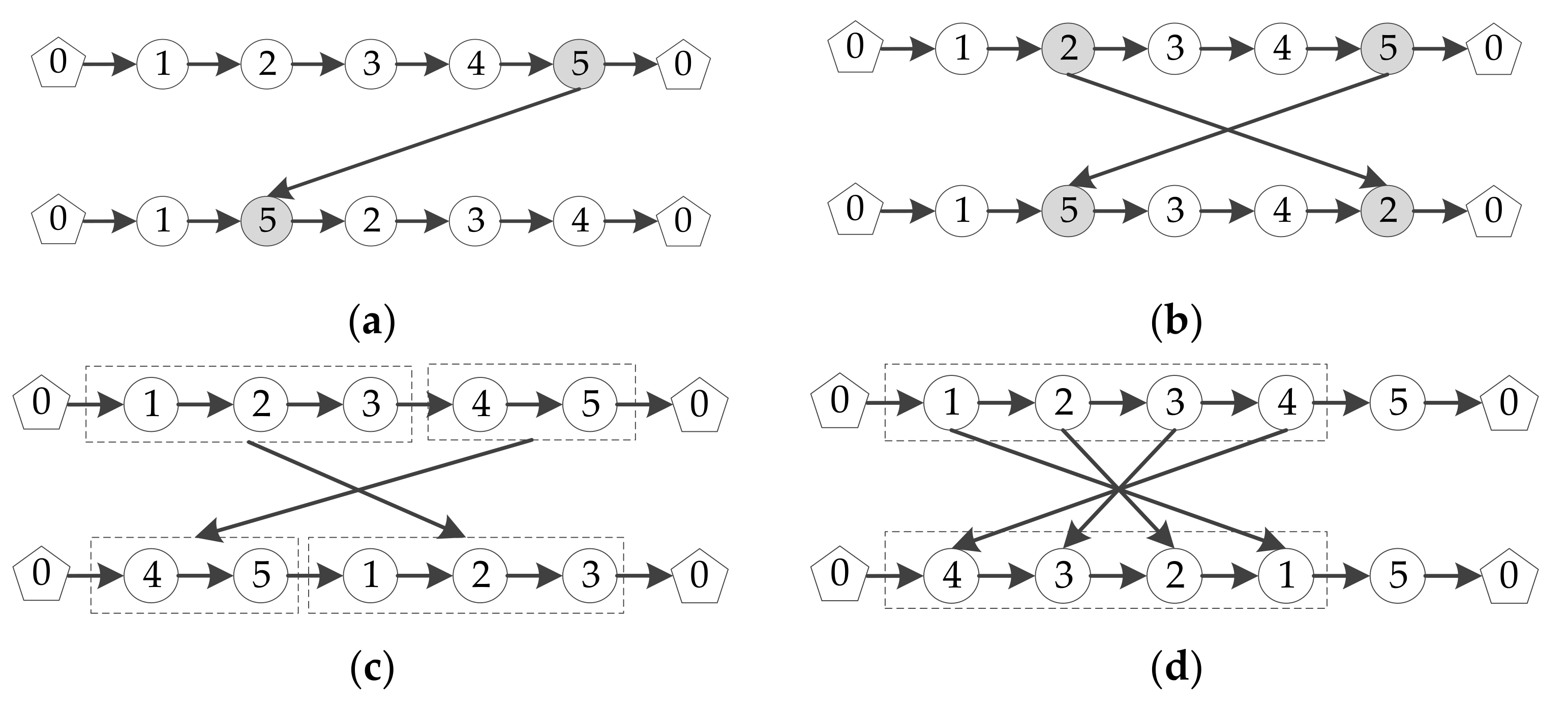
Four neighborhood structures are employed in our algorithm. In the procedure of SAVN, when a new solution is needed, one of these four structures is randomly selected with equal probability. As shown in Figure 2, all structures are described by an instance with 5 stations.

Neighborhood structure (a): A randomly selected station is relocated to another position in the current solution.

Neighborhood structure (b): Two randomly selected stations exchange their positions.

Neighborhood structure (c): Two randomly selected segments exchange their positions, and their lengths are at most 3.

Neighborhood structure (d): A pair of stations is randomly selected and all the stations between them, including themselves, are reversed.

5. Computational Results

5.1. Parameters and Experimental Data

We have implemented SAVN using MATLAB R2018a, and all computational experiments have been carried on an Intel Core i5-8259U with 2.3 GHz CPU and 8 GB RAM running the macOS Catalina operating system.

The test instances of BRP-MMFTR are generated randomly. The BSS stations’ coordinates are randomly generated in the range of abscissa [0,200] and ordinate [0,150]. The coordinate range of the traffic restricted area is the abscissa [80,160] and the ordinate [30,60]. The rebalancing demand of each BSS stations is randomly generated between [−20,20]. The depot coordinate is (100,75).

Table 2. Information of the depot, BSS stations and charging stations.

	X-Axis	Y-Axis	Demand	Index
Depot	100	75	0	0
BSS stations	86	143	−6	1
	75	35	3	2
	86	57	6	3
	99	36	11	4
	132	25	6	5
	138	44	−7	6
	108	18	−9	7
	100	98	−15	8
	172	60	6	9
	123	55	3	10
	110	128	16	11
	34	35	8	12
	161	112	−14	13
	140	103	7	14
	191	71	−12	15
	76	101	7	16
	48	118	5	17
	19	65	−4	18
Charging stations	30	66		C1
	48	35		C2
	126	73		C3
	52	101		C4
	145	27		C5

shows an example instance with one depot, 18 BSS stations and five charging stations. And

Table 3. Parameters of EVs and ICVs.

Vehicle Type	Maximum Mileage/km	Capacity	Fixed Cost/CNY	Traveling Energy Cost/(CNY·km−1)
EV	150	15	150	0.8
ICV	500	25	200	1.5

displays the parameters of EVs and ICVs. The other parameters used in BRP-MMFTR instances are as follows: R = 75 kW·h, $\mathit{r} = 0.5 \mathrm{kW}·\mathrm{h}/\mathrm{km}, \mathit{\mu }$ = 0.3, $\lambda$ = 0.5 kW·h/min, ${\mathit{C}}_{\mathit{w}}$ = 0.4 CNY/min, ${\mathit{C}}_{\mathit{L}}$ = 0.06 CNY/kg [34], and $L$ = 5 kg/km. Through preliminary tests, the parameters of SAVN are set as follows: ${\mathit{T}}_0$ = 50, $\alpha$ = 0.96, MaxUN = 50, and $\mathit{Len} = {\mathit{n}}^2$ (where, n is the number of BSS stations).

5.2. Comparisons of Computational Results

To verify the effectiveness of our SAVN, we compare it with SA and VNS (Variable Neighborhood Search) on the instance depicted above. Note that both SA and VNS use the same parameters of our SAVN. All the three algorithms were executed 10 times to weaken the randomness of the heuristic algorithm.

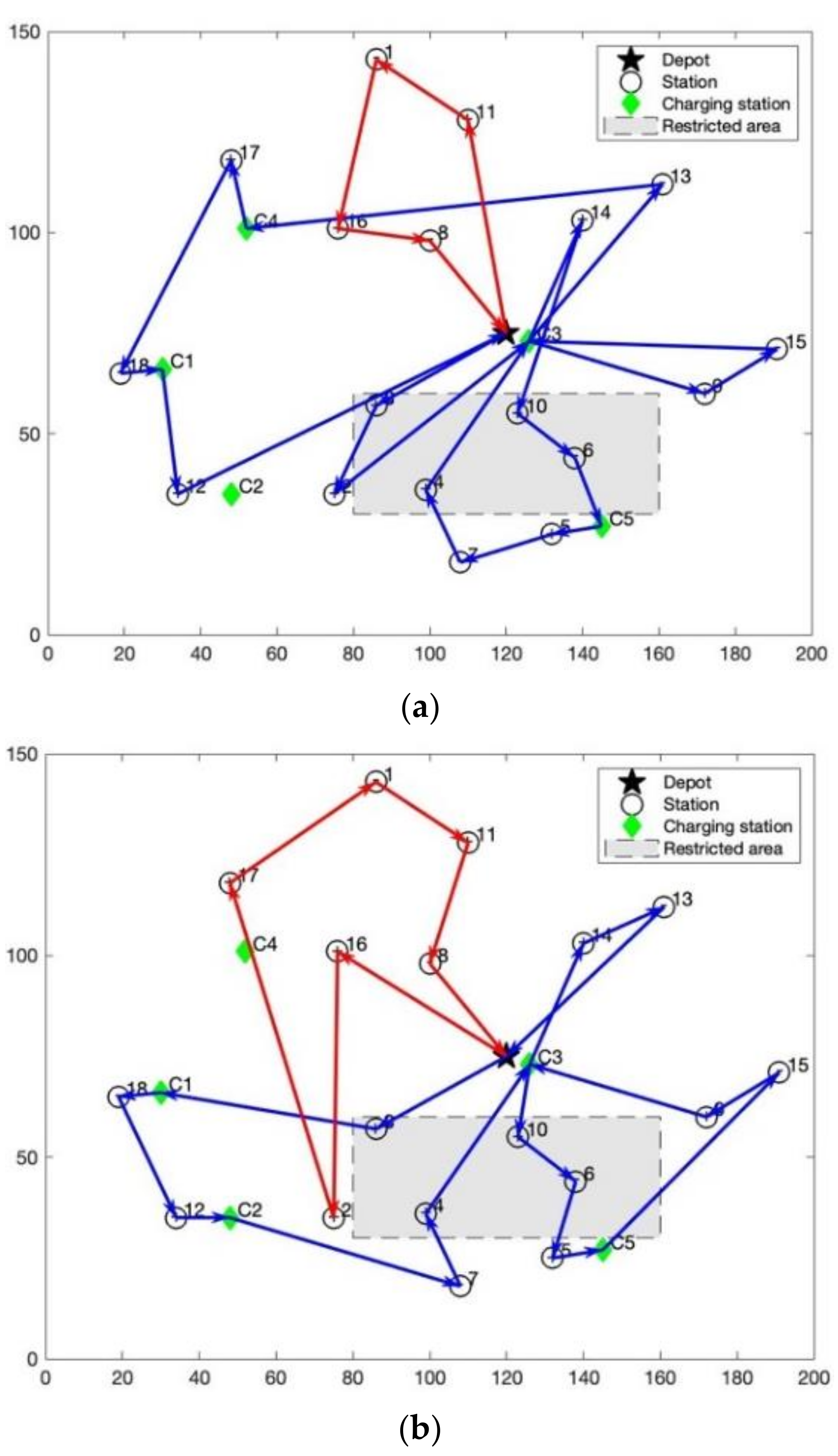
Figure 3 illustrates the vehicle routes obtained by SA, VNS and SAVN, respectively. The red lines represent the route of the ICV, while the blue lines represent the route of the EV. It can be observed that the solution obtained by SAVN has fewer detours, which make the vehicle’s travel distance smaller than those obtained by SA and VNS. Furthermore, its traveling energy costs, recharging costs and carbon emission costs can be also decreased.

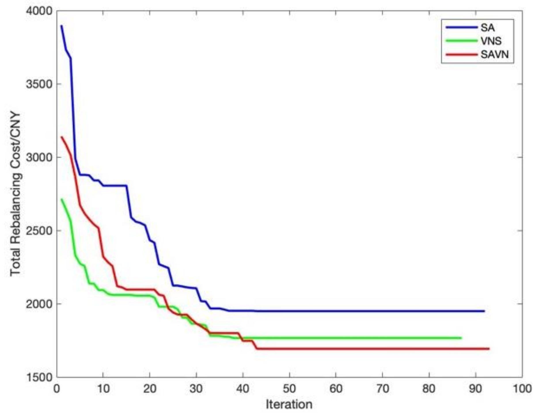
Figure 4 displays the comparison results of these algorithms. The X-coordinate is the number of iterations and the Y-coordinate is the total rebalancing cost. It can be seen that the final solution obtained by SAVN is better than SA and VNS, although in the early stage of the search process, SAVN may be inferior to VNS. This is due to the better optimization performance of SAVN, which can better escape from the trap of local optima. Hence, our SAVN can be regarded as an effective algorithm to solve BRP-MMFTR.

Table 4. Components of the total rebalancing cost in the optimal solution.

Costs/CNY	SA	VNS	SAVN
Fixed cost	350	350	350
Electricity cost of EV1	691	478	546
Fuel cost of ICV2	281	437	227
Recharging cost	571	414	524
Carbon emission cost	56	87	45
Total rebalancing cost	1949	1766	1692

Traveling energy cost is the sum of Electricity cost of EV¹ and Fuel cost of ICV².

lists the components of the total rebalancing cost in the BRP-MMFTR optimal solution obtained by SA, VNS, and SAVN. Obviously, for these three algorithms, SAVN is the best and SA is the worst for the total rebalancing cost. Although the electricity costs of EV obtained by SAVN is slightly worse than that of VNS, the fuel cost of ICV has been drastically reduced. In this way, SAVN’s traveling energy cost is less than VNS, because it is the sum of the electricity cost of EV and the fuel cost of ICV. Similarly, although SAVN’s recharging costs is higher than VNS for its EV has a longer travel distance, its carbon emission costs is lower. For practical BSS operators, SAVN’s solution is significantly better than VNS, because it employs EVs to perform more rebalancing operations. As we know, EVs are environmentally friendly and they will replace ICVs in the near future.

5.3. Computational Results of More Instances

To further verify the effectiveness and universality of SAVN, we tested the three algorithms in further instances. Theywere evaluated by nine test instances (three types, three instances per type), displayed in

Table 5. Nine instances of three types.

Instances	Small-Size			Medium-Size			Large-Size
	1	2	3	4	5	6	7	8	9
n	20	20	20	50	50	50	100	100	100
Depot	(100,75)
Abscissa range	[0,200]
Ordinate range	[0,150]
Demand range	[−20,20]

. The three types are small-size (n = 20), medium-size (n = 50) and large-size (n = 100). The instances are also generated randomly according to the method introduced in Section 5.1.

To provide reliable statistics, each algorithm is executed 10 times for each instance. And the average CPU time (t/s), the average total rebalancing cost (TRC) and the standard deviation (Sd) are displayed in

Table 6. Comparative results on nine instances.

Instances	Stations	SA			VNS			SAVN
		t/s	TRC	Sd	t/s	TRC	Sd	t/s	TRC	Sd
1	20	6.8	3071	29	8	2721	41	5.5	2669	13
2	20	8.4	2992	18	9.6	2917	33	9.4	2848	6
3	20	4.4	2402	30	7.4	2301	38	6.7	2162	16
4	50	44.6	5625	66	89.5	5220	58	115.6	5093	32
5	50	39.3	5452	58	88.3	4861	35	97.8	4720	31
6	50	32.4	6684	109	90.6	6214	60	66.4	6045	39
7	100	129.2	10733	144	508	9532	154	378.6	9072	63
8	100	185.6	10361	111	540.4	9510	80	394	9299	56
9	100	174.3	9920	105	448.5	8177	72	572.9	8032	13
Small	20	6.5	2821.7	25.6	8.3	2646.3	37.3	7.2	2559.7	11.7
Medium	50	38.8	5920.3	77.7	89.5	5431.7	51	93.3	5286	34
Large	100	163	10351.3	120	499	9073	102	448.5	8801	44

The best values are marked with bold.

. The best values are marked with bold fonts.

From Table 6, we can draw some conclusions as follows: For the average CPU time, SA has obvious advantages, but its solution quality is the worst. In addition, the calculation time of SAVN and VNS is difficult to distinguish the pros and cons. For the average total rebalancing cost, the solution obtained by SAVN can reduce 9.2% compared to SA or 3.4% compared to VNS in the small-size instances, 10.7% or 2.7% in the medium-size instances, and 15% or 3% in the large-size instances. With the number of stations increases, the solution quality of SAVN is getting better and better. Hence, from the perspective of solution quality and CPU time, SAVN can obtain a better solution than SA and VNS.

Furthermore, the standard deviation can reflect the stability of the algorithm. And the smaller the standard deviation is, the better the stability of the algorithm is. From Table 6, it is observed that the standard deviation of SAVN is the smallest in all the instances. Therefore, SAVN is more stable than the other two algorithms.

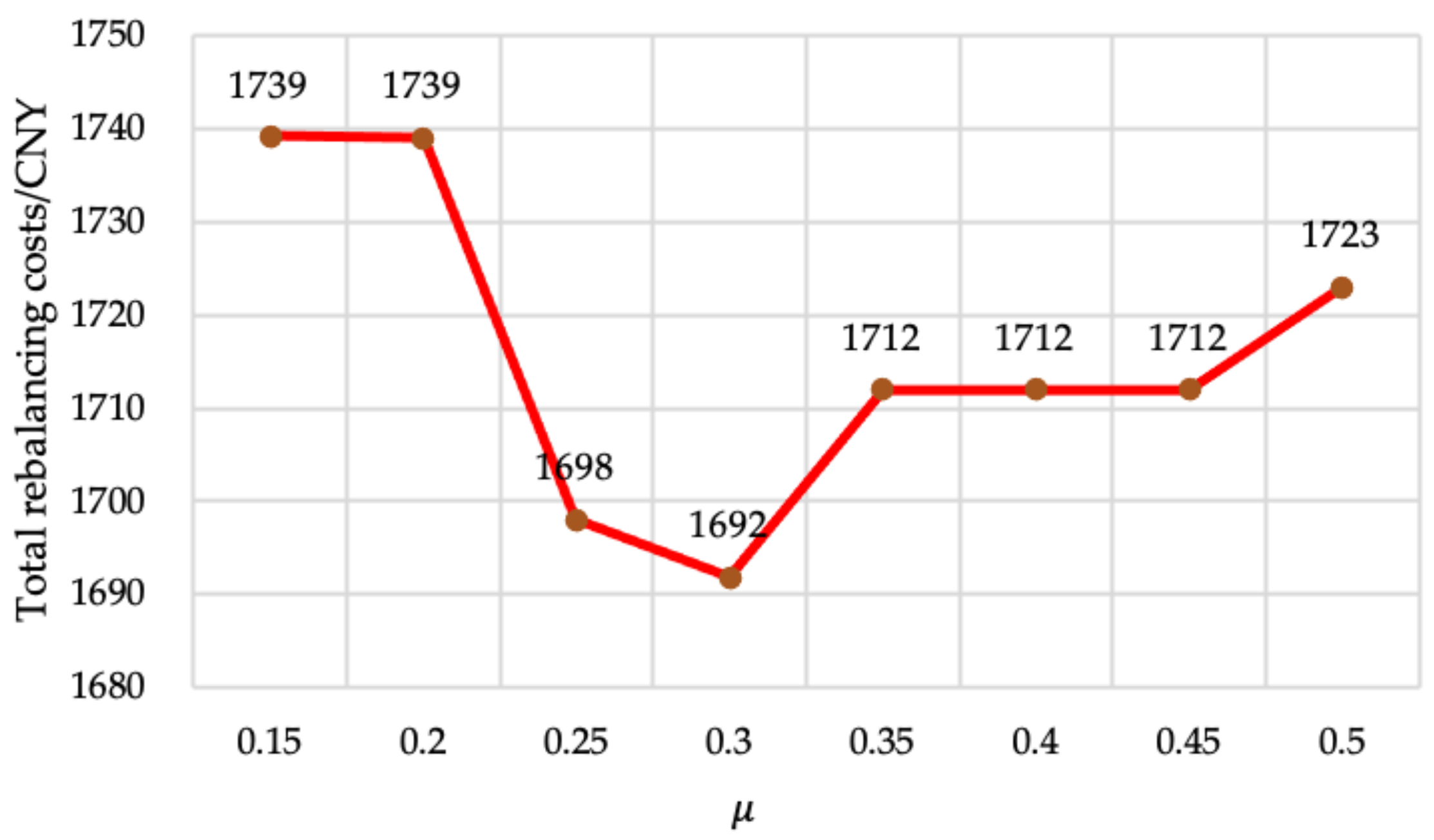
5.4. Discussion on the Value of μ

Parameter μ (the coefficient of safe-residual-charge level of EV) directly affects the charging time and then the recharging costs and the total travel distances. Hence, it is important to set a suitable value for μ. If the value of μ is set too low, there will be a probability of failing to drive to the nearest charging station. If the value of μ is set too high, the EV may frequently go to the charging station, which will cause a waste of energy and charging time. In this section, the sensitivity analysis of μ is analyzed using the 18-station instance in Section 5.2. The different values of μ are from 0.15 to 0.5 in increment of 0.05.

The SAVN is run 10 times for each μ and the trends of change with the increase of μ are illustrated in Figure 5. Obviously, the total rebalancing cost shows a clear trend of decreasing and then increasing. μ = 0.3 is the point with the lowest total rebalancing cost. In summary, parameter μ plays an important role in BRP-MMFTR and its value should be reasonably determined according to the layout of charging station system. If the quantity of charging stations is sufficient, the value of μ can be appropriately set lower. Otherwise, it should be set higher. Therefore, setting an appropriate value for μ is helpful to reduce the total rebalancing cost.

6. Conclusions

As a low-carbon and ecologically sustainable transportation mode, BSS has become a way to deal with the growing menace of global warming. In this study, we have proposed, modeled and solved BRP-MMFTR, which is a variant of BRP considering multi-energy mixed fleets and traffic restrictions. We first formulate BRP-MMFTR as a mixed integer programming model with the objective of minimizing the total rebalancing cost composed of vehicles’ fixed costs, vehicles’ traveling energy costs, EVs’ recharging costs, and ICVs’ carbon emission costs. Then SAVN is designed to solve this model, which is the simulated annealing algorithm enhanced with variable neighborhood structures. To illustrate the efficiency and efficacy of our algorithm, some test instances of BRP-MMFTR are generated randomly. The computational results reveal the huge advantage of SAVN, compared with SA and VNS. SAVN can achieve better solution in terms of solution quality and CPU time, outperforming those obtained by SA and VNS. In addition, SAVN is more stable than SA and VNS. Finally, the sensitivity analysis results of parameter μ indicate that as μ increases, the total rebalancing cost shows a clear trend of decreasing and then increasing. Therefore, setting an appropriate value for μ is helpful to reduce the total rebalancing cost. In addition, the value of μ is not necessarily constant in the practical rebalancing operations, and it can be dynamically adjusted according to the real-time conditions.

For BSS operators, we provide the optimal vehicle scheduling suggestions for multi-energy mixed fleets to minimize the total rebalancing cost when bike supply and user demand are not matched. In addition, we also focus on carbon emissions during the rebalancing process. BSS is originally a sustainable transportation mode, but if their operators use ICVs during rebalancing operations, the low-carbon benefits of BSS will be partially offset by the carbon emissions of ICVs. Therefore, it is obviously beneficial to create a green and low-carbon sustainable transportation system by using EVs instead of ICVs. The government should vigorously promote the sustainable development of EVs. Some policies, such as traffic restrictions on ICVs, can be introduced to encourage the BSS operators to purchase more EVs to minimize the carbon emissions.

Future research can extend our model and algorithm to solve more complex variants of BRP-MMFTR, such as considering the impact of average speed and speed variations to the traveling energy costs. Furthermore, dynamic or stochastic BRP-MMFTR is also a good research direction.

References

- Macioszek, E.; Świerk, P.; Kurek, A. The Bike-Sharing System as an Element of Enhancing Sustainable Mobility—A Case Study based on a City in Poland. Sustainability 2020, 12, 3285. [Google Scholar] [CrossRef] [Green Version]
- Song, M.; Wang, K.; Zhang, Y.; Li, M.; Qi, H.; Zhang, Y. Impact Evaluation of Bike-Sharing on Bicycling Accessibility. Sustainability 2020, 12, 6124. [Google Scholar] [CrossRef]
- Alvarez-Valdes, R.; Belenguer, J.M.; Benavent, E.; Bermudez, J.D.; Muñoz, F.; Vercher, E.; Verdejo, F. Optimizing the level of service quality of a bike-sharing system. Omega 2016, 62, 163–175. [Google Scholar] [CrossRef]
- Bruglieri, M.; Pezzella, F.; Pisacane, O. An Adaptive Large Neighborhood Search for relocating vehicles in electric carsharing services. Discret. Appl. Math. 2019, 253, 185–200. [Google Scholar] [CrossRef]
- Bulhões, T.; Subramanian, A.; Erdoğan, G.; Laporte, G. The static bike relocation problem with multiple vehicles and visits. Eur. J. Oper. Res. 2018, 264, 508–523. [Google Scholar] [CrossRef]
- Yang, X.-H.; Cheng, Z.; Chen, G.; Wang, L.; Ruan, Z.-Y.; Zheng, Y.-J. The impact of a public bicycle-sharing system on urban public transport networks. Transp. Res. Part A Policy Pract. 2018, 107, 246–256. [Google Scholar] [CrossRef]
- Nogal, M.; Jiménez, P. Attractiveness of Bike-Sharing Stations from a Multi-Modal Perspective: The Role of Objective and Subjective Features. Sustainability 2020, 12, 9062. [Google Scholar] [CrossRef]
- Fricker, C.; Gast, N. Incentives and redistribution in homogeneous bike-sharing systems with stations of finite capacity. Euro J. Transp. Logist. 2016, 5, 261–291. [Google Scholar] [CrossRef] [Green Version]
- Hiermann, G.; Puchinger, J.; Ropke, S.; Hartl, R.F. The Electric Fleet Size and Mix Vehicle Routing Problem with Time Windows and Recharging Stations. Eur. J. Oper. Res. 2016, 252, 995–1018. [Google Scholar] [CrossRef] [Green Version]
- Coelho, V.N.; Grasas, A.; Ramalhinho, H.; Coelho, I.M.; Souza, M.J.F.; Cruz, R.C. An ILS-based algorithm to solve a large-scale real heterogeneous fleet VRP with multi-trips and docking constraints. Eur. J. Oper. Res. 2016, 250, 367–376. [Google Scholar] [CrossRef] [Green Version]
- Erdoğan, G.; Laporte, G.; Wolfler Calvo, R. The static bicycle relocation problem with demand intervals. Eur. J. Oper. Res. 2014, 238, 451–457. [Google Scholar] [CrossRef] [Green Version]
- Dell’Amico, M.; Hadjicostantinou, E.; Iori, M.; Novellani, S. The bike sharing rebalancing problem: Mathematical formulations and benchmark instances. Omega 2014, 45, 7–19. [Google Scholar] [CrossRef]
- Cruz, F.; Subramanian, A.; Bruck, B.P.; Iori, M. A heuristic algorithm for a single vehicle static bike sharing rebalancing problem. Comput. Oper. Res. 2017, 79, 19–33. [Google Scholar] [CrossRef] [Green Version]
- Duan, Y.; Wu, J.; Zheng, H. A Greedy Approach for Vehicle Routing When Rebalancing Bike Sharing Systems. In Proceedings of the GLOBECOM 2018-2018 IEEE Global Communications Conference, Abu Dhabi, UAE, 9–13 December 2018. [Google Scholar]
- Casazza, M.; Ceselli, A.; Wolfler Calvo, R. A route decomposition approach for the single commodity Split Pickup and Split Delivery Vehicle Routing Problem. Eur. J. Oper. Res. 2021, 289, 897–911. [Google Scholar] [CrossRef]
- Papazek, P.; Kloimüllner, C.; Hu, B. Balancing Bicycle Sharing Systems: An Analysis of Path Relinking and Recombination within a GRASP Hybrid. In Parallel Problem Solving from Nature–PSN XIII; Bartz-eielstein, T., Ed.; Springer: Berlin/Heidelberg, Germany, 2014; pp. 792–801. [Google Scholar]
- Blesa, M.J.; Blum, C.; Festa, P. A Hybrid ACO+CP for Balancing Bicycle Sharing Systems. Hybrid Metaheuristics 2013, 198–212. [Google Scholar] [CrossRef]
- Raviv, T.; Kolka, O. Optimal inventory management of a bike-sharing station. Iie Trans. 2013, 45, 1077–1093. [Google Scholar] [CrossRef]
- Wang, Y.; Szeto, W.Y. Static green repositioning in bike sharing systems with broken bikes. Transp. Res. Part D Transp. Environ. 2018, 65, 438–457. [Google Scholar] [CrossRef]
- Usama, M.; Shen, Y.; Zahoor, O. Towards an Energy Efficient Solution for Bike-Sharing Rebalancing Problems: A Battery Electric Vehicle Scenario. Energies 2019, 12, 2503. [Google Scholar] [CrossRef] [Green Version]
- Pal, A.; Zhang, Y. Free-floating bike sharing: Solving real-life large-scale static rebalancing problems. Transp. Res. Part C Emerg. Technol. 2017, 80, 92–116. [Google Scholar] [CrossRef]
- Zhang, D.; Yu, C.; Desai, J.; Lau, H.Y.K.; Srivathsan, S. A time-space network flow approach to dynamic repositioning in bicycle sharing systems. Transp. Res. Part B Methodol. 2017, 103, 188–207. [Google Scholar] [CrossRef]
- Dell’Amico, M.; Iori, M.; Novellani, S.; Subramanian, A. The Bike sharing Rebalancing Problem with Stochastic Demands. Transp. Res. Part B Methodol. 2018, 118, 362–380. [Google Scholar] [CrossRef]
- Maggioni, F.; Cagnolari, M.; Bertazzi, L.; Wallace, S.W. Stochastic optimization models for a bike-sharing problem with transshipment. Eur. J. Oper. Res. 2019, 276, 272–283. [Google Scholar] [CrossRef]
- Yuan, M.; Zhang, Q.; Wang, B.; Liang, Y.; Zhang, H. A mixed integer linear programming model for optimal planning of bicycle sharing systems: A case study in Beijing. Sustain. Cities Soc. 2019, 47, 101515. [Google Scholar] [CrossRef]
- Legros, B. Dynamic repositioning strategy in a bike-sharing system; how to prioritize and how to rebalance a bike station. Eur. J. Oper. Res. 2019, 272, 740–753. [Google Scholar] [CrossRef]
- You, P.-S. A two-phase heuristic approach to the bike repositioning problem. Appl. Math. Model. 2019, 73, 651–667. [Google Scholar] [CrossRef]
- Correia, G.H.A.; Antunes, A.P. Optimization approach to depot location and trip selection in one-way carsharing systems. Transp. Res. Part E Logist. Transp. Rev. 2012, 48, 233–247. [Google Scholar] [CrossRef]
- Ons, S.; Wahiba, R.C.; Ammar, O. Vehicle Routing Problem with Mixed Fleet of Conventional and Heterogenous Electric Vehicles and Time Dependent Charging Costs. Technical Report. 2014. Available online: https://hal.archives-ouvertes.fr/hal-01083966 (accessed on 6 November 2020).
- Goeke, D.; Schneider, M. Routing a mixed fleet of electric and conventional vehicles. Eur. J. Oper. Res. 2015, 245, 81–99. [Google Scholar] [CrossRef]
- Macrina, G.; Di Puglia Pugliese, L.; Guerriero, F.; Laporte, G. The green mixed fleet vehicle routing problem with partial battery recharging and time windows. Comput. Oper. Res. 2019, 101, 183–199. [Google Scholar] [CrossRef]
- Hansen, P.; Mladenović, N.; Todosijević, R.; Hanafi, S. Variable neighborhood search: Basics and variants. Euro J. Comput. Optim. 2016, 5, 423–454. [Google Scholar] [CrossRef]
- Wei, L.; Zhang, Z.; Zhang, D.; Leung, S.C.H. A simulated annealing algorithm for the capacitated vehicle routing problem with two-dimensional loading constraints. Eur. J. Oper. Res. 2018, 265, 843–859. [Google Scholar] [CrossRef]
- China’s Seven Major Carbon Market K Line Chart. Available online: http://www.tanpaifang.com/tanhangqing/ (accessed on 25 October 2020).
Figure 1.
A schematic example of BRP-MMFTR.
Figure 2.
The neighborhood structures.
Figure 3.
Optimal vehicle routes obtained by three algorithms. (a) SA (b) VNS (c) SAVN.
Figure 4.
Comparison of total rebalancing cost.
Figure 5.
The trend of TRC changes with the increase of .