Article

Evaluation and Prediction of PM10 and PM2.5 from Road Source Emissions in Kuala Lumpur City Centre

by
Azliyana Azhari
1,*,
Nor Diana Abdul Halim
2,
Anis Asma Ahmad Mohtar
3,
Kadaruddin Aiyub
1,
Mohd Talib Latif
3 and
Matthias Ketzel
4,5
1
Center for Research in Development, Social and Environment, Faculty of Social Science and Humanities, Universiti Kebangsaan Malaysia, UKM Bangi 43600, Selangor, Malaysia
2
Institute for Environment and Development (LESTARI), Universiti Kebangsaan Malaysia, UKM Bangi 43600, Selangor, Malaysia
3
Department of Earth Sciences and Environment, Faculty of Science and Technology, Universiti Kebangsaan Malaysia, UKM Bangi 43600, Selangor, Malaysia
4
Department of Environmental Science, Aarhus University, Frederiksborgvej 399, DK-4000 Roskilde, Denmark
5
Global Centre for Clean Air Research (GCARE), Department of Civil and Environmental Engineering, University of Surrey, Guildford GU2 7XH, UK
*
Author to whom correspondence should be addressed.
Sustainability 2021, 13(10), 5402; https://0-doi-org.brum.beds.ac.uk/10.3390/su13105402
Submission received: 12 April 2021 / Revised: 4 May 2021 / Accepted: 5 May 2021 / Published: 12 May 2021

Abstract

:
Particulate matter (PM) is one of the major pollutants emitted by vehicles that adversely affect human health and the environment. This study evaluates and predicts concentrations and dispersion patterns of PM10 and PM2.5 in Kuala Lumpur city centre. The OML-Highway model calculates hourly time series of PM10 and PM2.5 concentrations and distribution caused by traffic emissions under different scenarios; business as usual (BAU) and 30% traffic reduction to see the impact of traffic reduction for sustainable traffic management. Continuous PM10 and PM2.5 data from a nearby monitoring station were analysed for the year 2019 and compared with modelled concentrations. Annual average concentration at various locations of interest for PM10 and PM2.5 during BAU runs were in the ranges 41.4–65.9 µg/m3 and 30.4–43.7 µg/m3 respectively, compared to during the 30% traffic reduction run ranging at 40.5–59.5 µg/m3 and 29.9–40.3 µg/m3 respectively. The average concentration of PM10 and PM2.5 at the Continuous Air Quality Monitoring Station (CAQMS) was 36.4 µg/m3 and 28.2 µg/m3 respectively. Strong correlations were observed between the predicted and observed data for PM10 and PM2.5 in both scenarios (p < 0.05). This research demonstrated that the reduction of traffic volume in the city contributes to reducing the concentration of particulate matter pollution.

1. Introduction

Particulate matter (PM) is one of the major air pollutants in cities that causes deterioration in air quality and is a threat to human health [1,2,3,4,5,6]. Most developing countries and megacities are struggling with increasing levels of ambient particulate matter and often violate World Health Organization (WHO) guidelines for PM concentrations [7]. PM emissions in the atmosphere are one of the most serious environmental issues. PM is also listed among the main pollutants contributing to variability in the Air Pollutant Index (API) [8]. Apart from the effects on air quality, PM has also been associated with mortality and respiratory diseases [9,10,11]. Burdens from diseases such as strokes, heart disease, lung cancer, and both chronic and acute respiratory disorders including asthma can be significantly reduced by lowering air pollution levels and a reduction of PM pollution [5,6,12]. PM emissions from vehicles depend on the type of engine and the age and maintenance of the vehicle (Pant and Harrison, 2013). Yan et al. (2011) showed that total emissions of PM can decrease 1.3–2.0% each year with controls and the introduction of better vehicles, proving that vehicular emissions play an important role in the global emissions of PM [13]. It was also revealed that vehicle fleets are the most influential factor contributing to the content of atmospheric PM, especially during weekdays [14,15]. The temporal variation of both traffic emissions and air dispersion parameters influences PM10 concentrations in the atmosphere [16,17].
Road traffic emissions have been one of the largest causes of environmental pollution, with a combination of different contaminants, including carbon monoxide (CO), nitrogen oxides (NOx), volatile organic compounds (VOCs) and PM [18,19,20,21]. Ideally, complete fossil fuel combustion will lead to the complete conversion of fuel into energy, but this is not feasible [22,23]. During combustion, disruptions happen and both unburned and partially burnt fuel will remain. In the process, impurities primarily mix with air to form other compounds, forming the partially burnt fuel and being converted into a variety of gases. Combustion products are primarily PM and gases, among the latter ozone precursors, including CO, NOx and VOCs, that are released as exhaust gases into the atmosphere [22]. With the increasing number of road traffic users to facilitate urbanization and industrialization processes, vehicular emissions are becoming the cause of air pollution problems [24]. Traffic-related air pollution measurements are difficult and costly to assess under real-world conditions [25] and so traffic pollution models are used as tools to calculate traffic emissions based on traffic data and vehicle-specific emission factors that depend on the type of vehicle and the driving conditions [26]. Modelling pollution dispersion can be useful to assess the impact of emissions on the environment and to assess human population exposure [27]. Using these models correctly will provide the closest estimation of real-world conditions of road traffic pollution. Previous research has modelled PM concentrations to evaluate the conditions of pollutants in the real world [19,28,29].
The Gaussian dispersion model has become a uniquely efficient tool for air quality management in recent decades and has been successfully used for a wide range of studies of air quality in urban and industrial areas [30,31]. Based on the Gaussian plume dispersion model principle, various types of air dispersion models have been designed and used in monitoring street pollution from vehicular sources. Among the popular models used are the Danish Operational Street Pollution Model (OSPM) [32,33], California Line Dispersion Model (CALINE) [34], Simple Evaluation Software for Atmospheric Pollutant Caused by Traffic (STREET 5) [35], and Atmospheric Dispersion Modelling System (ADMS) [36,37]. Various researchers have used different types of air dispersion models to study air pollution conditions with the aim of improving road traffic management in many ways [38,39,40]. Gulliver and Briggs (2011) developed STEMS-Air, a simple geographic information system (GIS)-based model to directly map air pollution at high spatial resolution and over large areas to produce daily or annual city-wide air pollution maps which can be used for urban air quality planning and management and health risk assessment. Traffic-related air pollution models can also be used in epidemiology studies to relate air pollution from road traffic to exposure to health effects (Shekarrizfard et al., 2015). Hertel et al. (2008) suggested based on OSPM calculations, that for bicyclists the choice a proper green route through a polluted city can significantly reduce air pollution exposure [41]. The OML-Highway model is a local-scale Gaussian air pollution model designed to describe the dispersion of air pollutants along roads with an open roadside environment [42]. It is designed for air quality assessment representing roads as area sources based on the OML model by Olesen et al. (2007) [43]. The OML-Highway model was integrated into SELMAGIS (Selma GIS system for air pollution modelling and visualization) to integrate sophisticated dispersion models into the framework with the ability to prepare input data and analyse model output data utilizing the spatial capabilities of GIS [42,44,45].
Adoption of the 2030 Agenda for Sustainable Development with the 17 Sustainable Development Goals (SDGs) has seen various efforts to tackle global development challenges including the issue of transport in urban areas. The objective of achieving environmental, economic and social sustainability can be achieved by a reduction in congestion and pollution [46]. Several researchers reviewed and discussed scenarios of pollution reduction towards environmental sustainability in specific cities [46,47]. In pursuit of achieving environmental sustainability goals, Russo and Comi (2016) suggested that implementing city logistic measures in a given city could improve the possibility of achieving the environmental goal. In attempting reduction of emission from road traffic in cities, several research studies discussed reduction, replacement and control of traffic volume [48,49,50]. Ho and Clappier (2011) discussed several measures for controlling air pollution from road traffic source by (i) control of the emission of all vehicles where all vehicles that do not meet the emissions standards must be upgraded or replaced, (ii) replacing 25% of the total number of motorcycle with public transport, and (iii) addition of more public transport and that will replace 50% of total motorcycles. It was learned that to keep the emission of Business as Usual scenario similar to the emission of reduction scenario, 45% of private vehicle have to be replaced by public transport [48]. Tezel-Oguz et al. (2020) applied NOx emissions inventory in the AERMOD model in five different emission reduction scenarios to observe the effects and exposure levels [50]. Steinberga et al. (2019) analysed five different scenarios including prioritization of public transport and restrictions of old private vehicles to reducing up to 50% of passenger vehicles using OSPM to calculate NOx and PM10 to minimize traffic-induced air pollution in street canyons [49].
The lack of comprehensive planning of a city, without consideration to social, economic, cultural, and environmental elements of the city results in a physical break of the community [51]. This paper focuses on predicting PM concentration and dispersion patterns in Kuala Lumpur city centre under different scenarios using the OML-Highway model, a local-scale Gaussian air pollution dispersion model. Two different scenarios were chosen, which were (i) business as usual (BAU) scenario which depicted the current situation of traffic flow and (ii) 30% traffic reduction in which the traffic flow was reduced by 30%. The prediction was then compared with observed data from a nearby Continuous Air Quality Monitoring Station (CAQMS) for validation. The results will be utilized to assess the relationship and effects of air pollution from road traffic emissions for sustainable city management.

2. Materials and Methods

2.1. Research Area

The study took place in Kuala Lumpur, the capital city of Malaysia. Kuala Lumpur is located on the west coast of the Malaysian Peninsula. Figure 1 shows the location of Kuala Lumpur city centre on the Malaysian Peninsula with target roads consisting of major roads and highways in Kuala Lumpur city centre and the CAQMS in Cheras, Kuala Lumpur. Kuala Lumpur is located on a flat area of land with an average elevation of 21.95 m above sea level while the range of elevation in the hilly areas of the city is 100–300 m above sea level. Kuala Lumpur covers a total land area of 243 km2 with a total population of 1.79 million in 2018 (Department of Statistics Malaysia, 2015). Kuala Lumpur has a strategic location at the heart of Peninsular Malaysia and is one of the country’s most developed and densely populated cities. The city is well connected to the surrounding areas by a highly developed transport network which includes highways, roads and railways [52]. Kuala Lumpur has undergone extensive expansion and experienced dramatic growth in development activities which has resulted in a continuous change of land use since its establishment [53]. As Kuala Lumpur is Malaysia’s most populous urbanized city and the country’s most important economic priority with extensive development of transport networks, it is the perfect location for this study.

2.2. Prediction and Forecast of Air Quality Dispersion

In achieving the goal of the study in evaluating and predicting PM10 and PM2.5 from road source emission, the application of the research process and the output of the study are depicted in Figure 2. Several considerations were made to develop the scenario in visualising how different conditions of road traffic can cause different levels of PM pollution in the city of Kuala Lumpur. In this study, two different scenarios were considered to compare the dispersion of PM during normal days in which the condition of road traffic are of no change in terms of legislation and infrastructure; and reducing by approximately 30% the amount of annual average daily traffic (AADT) on the road sections based on multiple discussions of reducing and/or replacing personal vehicles with public transport by 25–50% [48,49,50].
The OML-Highway model was applied to the sampling area to calculate the concentrations of PM10 originating from road traffic sources. The method used in this study was based on Olesen et al. (2015) with some modifications to meet the criteria of the Malaysian environment and traffic conditions as shown in Table 1. Traffic lanes were treated as area sources in OML-Highway. There are 4 highways and 37 trunk roads in Kuala Lumpur city centre which were selected as target roads as marked in red in Figure 1. The target roads used in the modelling were detailed with road network attributes including road type, annual average diurnal traffic (AADT), fractions of vehicle types, share of heavy-duty traffic and average travel speed as described in Table 1 and Figure 3. For the diurnal traffic variation and vehicle fleet emission factors, a standard set-up provided by OSPM tools was used and adapted to the conditions of the Malaysian environment and traffic by comparison with the emission factors produced by Đăng and Hùng (2014) and the emission inventories were modified from the Kuala Lumpur emission inventory by Azhari et al. (2021) [54,55]. Pollution concentrations were calculated at receptor points and visualized in SELMAGIS/ArcGIS software. Receptor points were generated along the road network at 10, 100, 200 and 300 m distances from the center of the road and at perpendicular transects in 100 m sections along the road network. Background PM10 and PM2.5 concentrations used in the OML-Highway calculations were taken from a background station run by the Department of Environment Malaysia in Banting, Selangor, a rural environment station with less influence of anthropogenic emissions, especially from road traffic. The meteorological data used in the modelling included wind direction, delta of wind direction, wind speed, humidity (percentage), cloud cover in eighths, rain, snow, temperature, global radiation, and estimated roughness length in a time series representing the meteorological conditions of the modelling area. The appropriate meteorological data used in this study were acquired from long-term monitoring by the Department of Environment Malaysia and the Malaysian Meteorological Department. The implementation of the OML-Highway in a GIS system enables visualization and evaluation of input and the calculation of the results in a simple and comprehensive way [46].

2.3. Continuous Air Quality Monitoring

Air quality data analysed in this research were collected from the Department of Environment CAQMS located at Sri Permaisuri Secondary School with coordinates 3.1062361° N, 101.7179167° E located about 10 km from Kuala Lumpur city centre. The CAQMS is located at a suburban school compound about 100 m from the closest suburban road. The hourly data of PM2.5 and PM10 were retrieved from DOE Malaysia for a duration of one year from January to December 2019. The PM10 and PM2.5 measurements presented in this paper were obtained using the Continuous Dichotomous Ambient Air Monitor 1405-DF Tapered Element Oscillating Microbalance (TEOMTM), which enables real-time measurements of mass concentrations of PM2.5 and PM10. Prior to submission to the Malaysian Department of Environment, the data went through thorough quality assurance and quality control (QA/QC) procedures. Flow verification for PM10 and PM2.5 measurements using the TEOM was conducted monthly as stipulated in the standard operating procedure for all instruments. Data omissions from the QC checks were primarily attributable to inadequate data (in turn due to negative values) and as a result of non-adherence to auto-calibration targets. On the second level of QC checks, data were omitted mainly due to outliers. Some of the observation data were rejected due to instrument failure and some were verified based on observed sources [56,57].

3. Results

Based on the input of average daily traffic, travel speed and share of heavy-duty vehicles, OML-Highway is able to model the dispersion of PM10 and PM2.5 from vehicular emissions based on fuel consumption and the meteorological data, provided that the regional background concentrations for these pollutants are available [42]. Comparison of average concentrations of pollutants from the modelled data and CAQMS are summarized in Table 2. The numbers present the annual average for 2019 and the standard deviation of the hourly values. The average modelled concentrations were 54.5 ± 27.8 µg/m3 and 50.76 ± 26.4 µg/m3 for the BAU scenario and 30% traffic reduction scenarios respectively, while the concentrations of PM10 at the CAQMS were recorded at 36.4 ± 24.2 µg/m3. The modelled concentrations of PM2.5 were 37.6 ± 24.3 µg/m3 for the BAU scenario and 35.3 ± 23.9 µg/m3 for the 30% traffic reduction scenario, while the concentrations of PM2.5 at the CAQMS were 28.2 ± 22.2 µg/m3. Figure 4 represents the comparison between the predicted concentrations from the model with observed data for PM10 and PM2.5. Good correlations were observed between the predicted and observed data: PM2.5 for BAU (r = 0.74, p < 0.05), PM2.5 for 30% traffic reduction (r = 0.75, p < 0.05), PM10 for BAU (r = 0.68, p < 0.05), and PM10 for 30% traffic reduction (r = 0.73, p < 0.05). Further ANOVA analysis using the Tukey’s test for post hoc analysis showed there were significant differences (p < 0.05) in the variation of PM10 and PM2.5 concentrations between the CAQMS, BAU scenario and 30% road traffic reduction scenario. The results show a significant correlation between modelled and observed data, although some over-predictions were observed as the modelled concentrations were slightly higher compared to observed data. This is likely to be because the predicted data were calculated at the receptor points closest to the road compared to the location of the CAQMS station for the observed data as the CAQMS station is the closest to the study area. Another plausible reason behind this trend is that the regional background data could have been overestimated for the model input [26,58].
Figure 5 shows the spatial concentration map of the annual means for PM10 and PM2.5 from OML-Highway for the BAU scenario and the 30% traffic reduction scenario. PM10 concentrations ranged from 41.4 to 65.9 µg/m3 with mean concentrations at the receptor points further away from the roadside (marked with a dark green marker) of 41.4–45.2 µg/m3 and at the receptor points closer to the roadside (red marker) with concentrations of 54.6–65.9 µg/m3. The concentrations of PM2.5 varied from 30.4 to 43.7 µg/m3 with the mean concentrations higher at the receptor points closer to the roadside having concentrations of 37.6–47.3 µg/m3 (marked with red markers) compared to the receptor points further away from the roadside with concentrations of 30.4–32.5 µg/m3 (marked with dark green markers). The results demonstrate that the concentrations of PM were higher in the city centre where the traffic density was higher. The pattern demonstrated that the concentrations of pollution from vehicle emissions were the highest close to the road source and are gradually dispersed by the wind and turbulent mixing further away from the centre of the road. The distribution of PM concentrations is highly associated with air dispersion and the movement of air masses [16,17]. ANOVA analysis using Tukey’s test for post hoc analysis showed there were significant differences (p < 0.05) in the variation of PM10 and PM2.5 concentrations in the distributions of the receptor point markers between the BAU scenario and 30% road traffic reduction scenario. The distributions of PM in the prediction for BAU are marked with more red and yellow markers compared with the predictions after 30% traffic reduction which are marked with yellow and green markers.
Figure 6 shows the diurnal variation of PM10 and PM2.5 concentrations from the OML-Highway prediction and CAQMS. The concentrations of PM10 and PM2.5 showed higher concentrations when modelled from the OML-Highway prediction compared with the observed data, usually, this was caused by overestimation of the dispersion at lower traffic volumes and lower emission values [26,58,59]. The diurnal variation of PM10 and PM2.5 from the BAU scenario and 30% traffic reduction scenario showed clear bimodal patterns with one peak in the morning and one peak in the night. The variations between the bimodal pattern from the modelled data compared with the trimodal pattern of the observed data are caused by the traffic patterns of the model input data [42]. The peak in the morning was associated with the morning rush hour traffic activities [1,17,60] and the peak in the night was associated with meteorological conditions such as atmospheric stability and wind speed [1]. The morning peak is more distinct than the evening peak as the morning rush hour is usually more concentrated as people try to get to work at almost the same time as compared with the evening rush hour which is more gradual. The diurnal variation in association with traffic flow with morning and evening maxima was also reported by Ferm and Sjöberg (2015). The differences in concentration ranges can be seen in both scenarios of OML model predictions for BAU and 30% road traffic reduction. The diurnal patterns for PM10 and PM2.5 concentrations for the observed data obtained from the CAQMS station showed trimodal distribution patterns. The concentrations of PM10 and PM2.5 significantly increased between 07:00 and 09:00 and decreased at midday, specifically after 11:00 (first peak). The second peak was recorded between 12:00 and 14:00. Then, the concentrations of PM10 and PM2.5 increased at 18:00 and began to decline after 02:00 (third peak). These three peaks can be attributed to the rush hour traffic that led to traffic being congested due to the higher number of vehicles on the road in Kuala Lumpur city centre in the early morning (first peak), afternoon (second peak) and late evening (third peak) associated with rush hour peaks as well as low mixing height that accumulated PM. The decline in the concentration after all the peaks was related to the decrease in vehicles on the road after the rush hour. According to Halim et al. (2020), Kuala Lumpur city centre is surrounded by main highways such as the KL-Putrajaya Highway, the DUKE Highway, the North–South Expressway, the Besraya Highway, and the SMART Tunnel as part of the programme road expansions linked with the urbanization process of the Kuala Lumpur Extended Mega Urban Regions (KLEMUR) [61]. The road expansion connected Kuala Lumpur city centre to the nearby urban cities via highways and led to congested and heavy traffic situations that increased emissions of PM10 and PM2.5 from the motor vehicles, especially from the exhaust and tyres [16,29,62,63].
The weekday variations of PM10 and PM2.5 concentrations in Kuala Lumpur city centre for the BAU scenario, 30% traffic reduction scenario and observed from CAQMS, depicted in Figure 7, demonstrate that the variations are mostly similar on all days of the week. The concentrations of PM10 and PM2.5 were recorded to be higher on Mondays and on Thursdays and Fridays in Kuala Lumpur city centre, while the concentrations of both air pollutants remained low at the weekends. Further ANOVA analysis using Tukey’s test for post hoc analysis showed there were significant differences (p < 0.05) in the weekly variation of PM10 and PM2.5 concentrations between the CAQMS, BAU scenario and 30% road traffic reduction scenario. This clearly indicated that motor vehicles did contribute to the higher concentrations of PM10 and PM2.5 on weekdays and the lesser movement of motor vehicles at weekends led to a reduction of PM10 and PM2.5. This was likely to have been due to the higher number of vehicles on the main highway that connected Kuala Lumpur city centre to nearby cities. The vigorous economic growth of Kuala Lumpur city centre resulted in most of the city centre being used for business purposes until urban sprawl was induced to the southern part of Kuala Lumpur due to accommodation demands in the affordable areas [64]. This situation led to congested flows of traffic on Mondays, Thursdays and Fridays as many employees that work in Kuala Lumpur travel back home to the nearest cities located outside of the Kuala Lumpur region since Kuala Lumpur city centre is well known to be one of the main cities in Malaysia offering more job opportunities. In addition, the increase in private vehicle ownership has resulted in Kuala Lumpur city centre being ranked as having one of the lowest levels of public transport participation in Asia since rapid motorization in the 1980s [65,66].
Monthly variations of PM10 and PM2.5 concentrations for the BAU scenario, 30% traffic reduction scenario and observed from CAQMS in Kuala Lumpur city centre are presented in Figure 8. The monthly concentrations of PM during the 30% road traffic reduction scenario are not very different from those during the BAU scenario. The concentrations of PM10 and PM2.5 were 100 µg/m3 and 80 µg/m3 respectively during the BAU scenario while during 30% road traffic reduction, the concentrations of PM10 and PM2.5 approached 100 µg/m3 and 80 µg/m3 respectively. ANOVA analysis using Tukey’s test for post hoc analysis showed there were significant differences (p < 0.05) in the monthly variation of PM10 and PM2.5 concentrations between the CAQMS, BAU scenario and 30% road traffic reduction scenario. This shows that the monthly variations of PM depended more on the seasonal fluctuations and regional transportation of PM compared with the diurnal and weekly variations that depended on traffic emissions. The monthly variations in PM10 and PM2.5 concentrations from the CAQMS showed that the concentrations were influenced by the monsoon seasons. The annual variation of PM10 and PM2.5 indicated higher PM concentrations in September which is the dry season in Malaysia and is associated with transboundary pollutants, especially from Indonesia [8,67,68,69]. The findings in this study were similar to previous studies reported by Anwar et al. (2010), Juneng et al. (2011) and Latif et al. (2014) as the monthly concentrations for both air pollutants were recorded at higher concentrations during seasonal monsoon periods, especially during the northeast (NE) monsoon (late November to March) and the southwest (SW) monsoon (late May to September) [4,17,70,71]. The higher concentrations of PM10 and PM2.5 during the seasonal monsoons are due to the movement of air mass particles which mainly consist of particulate matter that typically originated from biomass burning activities from nearby regions such as Sumatra and Indo-China [4,17,69,72,73].
The variation in concentrations between the modelled data and observed data takes into consideration that the receptor points are closer to the road source compared to the monitoring station location. It was depicted that road traffic was a major source of particulate matter pollution in cities through the clear pattern of reduction in concentrations of PM10 and PM2.5 between the BAU scenario and 30% reduction of traffic volume scenario [49,50]. The distribution patterns of particulate matter showed that the concentrations of PM10 and PM2.5 were generally higher closer to the source of pollutants, the centre of the road. The concentrations of PM are highly associated with air dispersion and the movements of air masses [16,17]. Despite the fact that traffic networking is one of the most important factors in supporting the urbanization process and the population, it is also becoming one of the major sources of air pollutants that cause both environmental and health issues including changes to urban and global air quality and climate, infrastructure damage, impacts to vegetation, and direct and indirect health problems [74,75,76]. A better option for sustainable road traffic management is needed to control the air pollution impact from road traffic emissions [77,78]. The transportation sector is proven to be one of the critical sectors in environmental management in the pursuit of sustainable development. An environment-friendly transportation network is one of the key points in achieving a sustainably developed and liveable city [79,80,81]. There is a need to solve the issue as the condition of the current environmental state will have negative effects on human health and ecosystems, hence will affect the liveability and sustainability of the surrounding area. Effective road traffic management, through a reduction in traffic volume or various restrictions through imposed policies and rules, will aid in minimizing traffic-induced air pollution [49,50]. It is important to establish a strategy to reduce pollution and improve road traffic to help reduce air pollution and promote a healthy atmosphere for urban dwellers.

4. Conclusions

This study demonstrated that PM pollutants in urban areas are greatly contributed to by vehicle emissions. Based on the continuous air quality monitoring data, the results demonstrated that the levels of PM2.5 at the CAQMS were 28.2 ± 22.2 µg/m3 while the average concentration of PM10 was 36.4 ± 24.2 µg/m3. The diurnal and weekday variations of PM concentrations from the observed data showed that the concentrations of PM were highly attributed to vehicle emissions and traffic volume. Apart from vehicle emissions, PM10 concentrations were also influenced by other factors including monsoon season variations and air mass movements, which also impact the long-range dispersion of PM10 pollutants. The average concentrations of predicted PM2.5 were 37.6 ± 24.3 µg/m3 and 35.3 ± 23.9 µg/m3 for the BAU and 30% traffic reduction scenarios respectively, while average concentrations of PM10 were 54.5 ± 27.8 µg/m3 and 50.8 ± 26.4 µg/m3 for the BAU and 30% traffic reduction scenarios respectively. The predicted concentrations of PM from the model correlated with the observed concentrations were as follows: PM2.5 for BAU (r = 0.74, p < 0.05), PM2.5 for 30% traffic reduction (r = 0.75, p < 0.05), PM10 for BAU (r = 0.68, p < 0.05), and PM10 for 30% traffic reduction (r = 0.73, p < 0.05). Even though traffic networking is one of the most important factors in supporting the population, increasing air pollution causes adverse effects on the wellbeing of the urban population. A better option for sustainable road traffic management is needed to control the air pollution impacts from road traffic emissions and to establish a better environment for the urban population.

Author Contributions

Conceptualization, A.A., K.A. and M.T.L.; methodology, A.A., N.D.A.H. and A.A.A.M.; software, A.A. and M.K.; validation, M.K.; formal analysis, A.A., N.D.A.H. and A.A.A.M.; writing—original draft preparation, A.A., N.D.A.H. and A.A.A.M.; writing—review and editing, K.A., M.T.L. and M.K.; supervision, K.A., M.T.L. and M.K.; project administration, A.A. and K.A. All authors have read and agreed to the published version of the manuscript.

Funding

This research was funded by Universiti Kebangsaan Malaysia, grant number MI-2020-011.

Institutional Review Board Statement

Not applicable.

Informed Consent Statement

Not applicable.

Data Availability Statement

The data presented in this study are available on request from the corresponding author.

Acknowledgments

The authors would like to express their extreme gratitude to the Malaysian Department of the Environment (DOE), the Ministry of Works (KKR) and Integrated Transportation Information System (ITIS), Kuala Lumpur City Hall (DBKL) Malaysia for permission to use their air quality data, industrial emissions data, and traffic data. Special thanks to Dr Rose Norman for proofreading this manuscript.

Conflicts of Interest

The authors declare no conflict of interest.

References

  1. Afroz, R.; Hassan, M.N.; Ibrahim, N.A. Review of air pollution and health impacts in Malaysia. Environ. Res. 2003, 92, 71–77. [Google Scholar] [CrossRef]
  2. Chen, S.-C.; Liao, C.-M. Health risk assessment on human exposed to environmental polycyclic aromatic hydrocarbons pollution sources. Sci. Total Environ. 2006, 366, 112–123. [Google Scholar] [CrossRef] [PubMed]
  3. Duan, J.; Chen, Y.; Fang, W.; Su, Z. Characteristics and Relationship of PM, PM10, PM2.5 Concentration in a Polluted City in Northern China. Procedia Eng. 2015, 102, 1150–1155. [Google Scholar] [CrossRef] [Green Version]
  4. Juneng, L.; Latif, M.T.; Tangang, F. Factors influencing the variations of PM10 aerosol dust in Klang Valley, Malaysia during the summer. Atmos. Environ. 2011, 45, 4370–4378. [Google Scholar] [CrossRef]
  5. Lurie, K.; Nayebare, S.R.; Fatmi, Z.; Carpenter, D.O.; Siddique, A.; Malashock, D.; Khan, K.; Zeb, J.; Hussain, M.M.; Khatib, F.; et al. PM2.5 in a megacity of Asia (Karachi): Source apportionment and health effects. Atmos. Environ. 2019, 202, 223–233. [Google Scholar] [CrossRef]
  6. Zhang, P.; Zhou, X. Health and economic impacts of particulate matter pollution on hospital admissions for mental disorders in Chengdu, Southwestern China. Sci. Total Environ. 2020, 733, 139114. [Google Scholar] [CrossRef]
  7. Gulia, S.; Nagendra, S.S.; Khare, M.; Khanna, I. Urban air quality management-A review. Atmos. Pollut. Res. 2015, 6, 286–304. [Google Scholar] [CrossRef] [Green Version]
  8. Dominick, D.; Juahir, H.; Latif, M.T.; Zain, S.M.; Aris, A.Z. Spatial assessment of air quality patterns in Malaysia using multivariate analysis. Atmos. Environ. 2012, 60, 172–181. [Google Scholar] [CrossRef]
  9. Chen, J.; Li, C.; Ristovski, Z.; Milic, A.; Gu, Y.; Islam, M.S.; Wang, S.; Hao, J.; Zhang, H.; He, C.; et al. A review of biomass burning: Emissions and impacts on air quality, health and climate in China. Sci. Total Environ. 2017, 579, 1000–1034. [Google Scholar] [CrossRef] [Green Version]
  10. ChooChuay, C.; Pongpiachan, S.; Tipmanee, D.; Suttinun, O.; Deelaman, W.; Wang, Q.; Xing, L.; Li, G.; Han, Y.; Palakun, J.; et al. Impacts of PM2.5 sources on variations in particulate chemical compounds in ambient air of Bangkok, Thailand. Atmos. Pollut. Res. 2020, 11, 1657–1667. [Google Scholar] [CrossRef]
  11. Mahiyuddin, W.R.W.; Sahani, M.; Aripin, R.; Latif, M.T.; Thach, T.-Q.; Wong, C.-M. Short-term effects of daily air pollution on mortality. Atmos. Environ. 2013, 65, 69–79. [Google Scholar] [CrossRef]
  12. Teixeira, A.C.R.; Borges, R.R.; Machado, P.G.; Mouette, D.; Ribeiro, F.N.D. PM emissions from heavy-duty trucks and their impacts on human health. Atmos. Environ. 2020, 241, 117814. [Google Scholar] [CrossRef]
  13. Yan, F.; Winijkul, E.; Bond, T.C.; Streets, D.G. Global emission projections of particulate matter (PM): II Uncertainty analyses of on-road vehicle exhaust emissions. Atmos. Environ. 2014, 87, 189–199. [Google Scholar] [CrossRef]
  14. Piras, G.; Pini, F.; Garcia, D.A. Correlations of PM10 concentrations in urban areas with vehicle fleet development, rain precipitation and diesel fuel sales. Atmos. Pollut. Res. 2019, 10, 1165–1179. [Google Scholar] [CrossRef]
  15. Pongpiachan, S.; Kositanont, C.; Palakun, J.; Liu, S.; Ho, K.F.; Cao, J. Effects of day-of-week trends and vehicle types on PM2.5-bounded carbonaceous compositions. Sci. Total Environ. 2015, 532, 484–494. [Google Scholar] [CrossRef] [PubMed]
  16. Ferm, M.; Sjöberg, K. Concentrations and emission factors for PM 2.5 and PM 10 from road traffic in Sweden. Atmos. Environ. 2015, 119, 211–219. [Google Scholar] [CrossRef]
  17. Latif, M.T.; Dominick, D.; Ahamad, F.; Khan, F.; Juneng, L.; Hamzah, F.M.; Nadzir, M.S.M. Long term assessment of air quality from a background station on the Malaysian Peninsula. Sci. Total Environ. 2014, 482-483, 336–348. [Google Scholar] [CrossRef] [PubMed]
  18. Jaiprakash; Habib, G.; Kumar, A.; Sharma, A.; Haider, M. On-road emissions of CO, CO2 and NOX from four wheeler and emission estimates for Delhi. J. Environ. Sci. 2017, 53, 39–47. [Google Scholar] [CrossRef]
  19. Lawrence, S.; Sokhi, R.; Ravindra, K. Quantification of vehicle fleet PM10 particulate matter emission factors from exhaust and non-exhaust sources using tunnel measurement techniques. Environ. Pollut. 2016, 210, 419–428. [Google Scholar] [CrossRef]
  20. Mao, J.; Yang, L.; Mo, Z.; Jiang, Z.; Krishnan, P.; Sarkar, S.; Zhang, Q.; Chen, W.; Zhong, B.; Yang, Y.; et al. Comparative study of chemical characterization and source apportionment of PM2.5 in South China by filter-based and single particle analysis. Elem. Sci. Anth. 2021, 9. [Google Scholar] [CrossRef]
  21. Nagpure, A.S.; Gurjar, B.; Kumar, V.; Kumar, P. Estimation of exhaust and non-exhaust gaseous, particulate matter and air toxics emissions from on-road vehicles in Delhi. Atmos. Environ. 2016, 127, 118–124. [Google Scholar] [CrossRef]
  22. Dewangan, A.; Mallick, A.; Yadav, A.K.; Kumar, R. Combustion-generated pollutions and strategy for its control in CI engines: A review. Mater. Today Proc. 2020, 21, 1728–1733. [Google Scholar] [CrossRef]
  23. Lewtas, J. Air pollution combustion emissions: Characterization of causative agents and mechanisms associated with cancer, reproductive, and cardiovascular effects. Mutat. Res. 2007, 636, 95–133. [Google Scholar] [CrossRef] [PubMed]
  24. Luken, R.A.; Van Berkel, R.; Leuenberger, H.; Schwager, P. A 20-year retrospective of the National Cleaner Production Centres programme. J. Clean. Prod. 2016, 112, 1165–1174. [Google Scholar] [CrossRef]
  25. Carslaw, D.C.; Rhys-Tyler, G. New insights from comprehensive on-road measurements of NOx, NO2 and NH3 from vehicle emission remote sensing in London, UK. Atmos. Environ. 2013, 81, 339–347. [Google Scholar] [CrossRef] [Green Version]
  26. Berkowicz, R.; Ketzel, M.; Jensen, S.S.; Hvidberg, M.; Raaschou-Nielsen, O. Evaluation and application of OSPM for traffic pollution assessment for a large number of street locations. Environ. Model. Softw. 2008, 23, 296–303. [Google Scholar] [CrossRef]
  27. Amirjamshidi, G.; Mostafa, T.S.; Misra, A.; Roorda, M.J. Integrated model for microsimulating vehicle emissions, pollutant dispersion and population exposure. Transp. Res. Part D Transp. Environ. 2013, 18, 16–24. [Google Scholar] [CrossRef]
  28. Assael, M.; Delaki, M.; Kakosimos, K. Applying the OSPM model to the calculation of PM10 concentration levels in the historical centre of the city of Thessaloniki. Atmos. Environ. 2008, 42, 65–77. [Google Scholar] [CrossRef]
  29. Ketzel, M.; Omstedt, G.; Johansson, C.; Düring, I.; Pohjolar, M.; Oettl, D.; Gidhagen, L.; Wåhlin, P.; Lohmeyer, A.; Haakana, M.; et al. Estimation and validation of PM2.5/PM10 exhaust and non-exhaust emission factors for practical street pollution modelling. Atmos. Environ. 2007, 41, 9370–9385. [Google Scholar] [CrossRef]
  30. Awasthi, S.; Khare, M.; Gargava, P. General plume dispersion model (GPDM) for point source emission. Environ. Model. Assess. 2006, 11, 267–276. [Google Scholar] [CrossRef]
  31. Brusca, S.; Famoso, F.; Lanzafame, R.; Mauro, S.; Garrano, A.M.C.; Monforte, P. Theoretical and Experimental Study of Gaussian Plume Model in Small Scale System. Energy Procedia 2016, 101, 58–65. [Google Scholar] [CrossRef]
  32. Berkowicz, R. OSPM—A parameterised street polluton model. Environ. Monit. Assess. 2000, 65, 323–331. [Google Scholar] [CrossRef]
  33. Lazić, L.; Urošević, M.A.; Mijić, Z.; Vuković, G.; Ilić, L. Traffic contribution to air pollution in urban street canyons: Integrated application of the OSPM, moss biomonitoring and spectral analysis. Atmos. Environ. 2016, 141, 347–360. [Google Scholar] [CrossRef]
  34. Benson, P.E. CALINE4—A Dispersion Model for Predicting Air Pollutant Concentration Near Roadways; California Department of Transportation, Office of Transportation Laboratory: Sacramento, CA, USA, 1984. [Google Scholar]
  35. Pénard-Morand, C.; Schillinger, C.; Armengaud, A.; Debotte, G.; Chrétien, E.; Pellier, S.; Annesi-Maesano, I. Assessment of schoolchildren’s exposure to traffic-related air pollution in the French Six Cities Study using a dispersion model. Atmos. Environ. 2006, 40, 2274–2287. [Google Scholar] [CrossRef]
  36. Beevers, S.D.; Kitwiroon, N.; Williams, M.L.; Carslaw, D.C. One way coupling of CMAQ and a road source dispersion model for fine scale air pollution predictions. Atmos. Environ. 2012, 59, 47–58. [Google Scholar] [CrossRef]
  37. Dėdelė, A.; Miškinytė, A. Seasonal and site-specific variation in particulate matter pollution in Lithuania. Atmos. Pollut. Res. 2019, 10, 768–775. [Google Scholar] [CrossRef]
  38. Gulliver, J.; Briggs, D. STEMS-Air: A simple GIS-based air pollution dispersion model for city-wide exposure assessment. Sci. Total Environ. 2011, 409, 2419–2429. [Google Scholar] [CrossRef] [PubMed]
  39. Sofia, D.; Gioiella, F.; Lotrecchiano, N.; Giuliano, A. Mitigation strategies for reducing air pollution. Environ. Sci. Pollut. Res. 2020, 27, 19226–19235. [Google Scholar] [CrossRef]
  40. Tang, J.; McNabola, A.; Misstear, B. The potential impacts of different traffic management strategies on air pollution and public health for a more sustainable city: A modelling case study from Dublin, Ireland. Sustain. Cities Soc. 2020, 60, 102229. [Google Scholar] [CrossRef]
  41. Hertel, O.; Hvidberg, M.; Ketzel, M.; Storm, L.; Stausgaard, L. A proper choice of route significantly reduces air pollution exposure—A study on bicycle and bus trips in urban streets. Sci. Total Environ. 2008, 389, 58–70. [Google Scholar] [CrossRef]
  42. Olesen, H.R.; Ketzel, M.; Jensen, S.S.; Løfstrøm, P.; Im, U.; Becker, T. User Guide to OML-Highway. In A Tool for Air Pollution Assessments along Highways; Aarhus University, DCE—Danish Centre for Environment and Energy: Aarhus, Denmark, 2015; p. 66. [Google Scholar]
  43. Olesen, H.R.; Berkowicz, R.; Løfstrøm, P. OML: Review of Model Formulation; National Environmental Research Institute: Aarhus, Denmark, 2007. [Google Scholar]
  44. Becker, T.; Ketzel, M.; Løfstrøm, P.; Lorentz, H.; Jensen, S.S.; Olesen, H.R. OML-Highway—A Road source model in a GIS environment—evaluation with measurements In Proceedings of the 13th Conference on Harmonisation within Atmospheric Dispersion Modelling for Regulatory Purposes, Paris, France, 1–4 June 2010.
  45. Jensen, S.S.; Becker, T.; Ketzel, M.; Løfstrøm, P.; Olesen, H.R.; Lorentz, H. OML-Highway within the Framework of SELMA-GIS; National Environmental Research Institute, Aarhus University: Aarhus, Denmark, 2010; p. 26. [Google Scholar]
  46. Russo, F.; Comi, A. Urban Freight Transport Planning towards Green Goals: Synthetic Environmental Evidence from Tested Results. Sustainability 2016, 8, 381. [Google Scholar] [CrossRef] [Green Version]
  47. Meyer, T. Decarbonizing road freight transportation—A bibliometric and network analysis. Transp. Res. Part D Transp. Environ. 2020, 89, 102619. [Google Scholar] [CrossRef]
  48. Ho, B.Q.; Clappier, A. Road traffic emission inventory for air quality modelling and to evaluate the abatement strategies: A case of Ho Chi Minh City, Vietnam. Atmos. Environ. 2011, 45, 3584–3593. [Google Scholar] [CrossRef]
  49. Steinberga, I.; Susterea, L.; Bikse, J.; Bilkse, J.B., Jr.; Kleperis, J. Traffic induced air pollution modeling: Scenario analysis for air quality management in street canyon. Procedia Comput. Sci. 2019, 149, 384–389. [Google Scholar] [CrossRef]
  50. Tezel-Oguz, M.N.; Sari, D.; Ozkurt, N.; Keskin, S.S. Application of reduction scenarios on traffic-related NOx emissions in Trabzon, Turkey. Atmos. Pollut. Res. 2020, 11, 2379–2389. [Google Scholar] [CrossRef]
  51. Pardo, C.F.; Jiemian, Y.; Hongyuan, Y.; Mohanty, C.R. Sustainable urban transport. In Shanghai Manual—A Guide for Sustainable Urban Development in the 21st Century; United Nations: Shanghai, China, 2011; pp. 106–143. [Google Scholar]
  52. Hadi, A.S.; Idrus, S.; Shah, A.H.H.; Mohamed, A.F. Critical Urbanisation Transitions in Malaysia: The Challenge of Rising Bernam to Linggi Basin Extended Mega Urban Region. Akademika 2011, 81, 10. [Google Scholar]
  53. Asnawi, N.H.; Ahmad, P.; Choy, L.K.; Khair, M.S.A.A. Land use and land cover change in Kuala Lumpur using remote sensing and geographic information system approach. J. Built Environ. Technol. Eng. 2018, 4, 10. [Google Scholar]
  54. Azhari, A.; Halim, N.D.A.; Othman, M.; Latif, M.T.; Juneng, L.; Sofwan, N.M.; Stocker, J.; Johnson, K. Highly spatially resolved emission inventory of selected air pollutants in Kuala Lumpur’s urban environment. Atmos. Pollut. Res. 2021, 12, 12–22. [Google Scholar] [CrossRef]
  55. Đăng, P.N.; Hùng, N.T. Thematic Report on Traffic Emission Coefficient for Hanoi, Vietnam; Center for Environment of Towns and Industrial Areas: Hanoi, Vietnam, 2014. [Google Scholar]
  56. PSTW. CAQMS—Standard Operating Procedures for Operation, Scheduled, Maintenance, Troubleshooting, Calibration and Verification; PSTW: Shah Alam, Malaysia, 2018. [Google Scholar]
  57. PSTW. MAQM—Standard Operating Procedures for Operation, Scheduled, Maintenance, Troubleshooting and Verification; PSTW: Shah Alam, Malaysia, 2018. [Google Scholar]
  58. Amoatey, P.; Omidvarborna, H.; Baawain, M.S.; Al-Mamun, A. Evaluation of vehicular pollution levels using line source model for hot spots in Muscat, Oman. Environ. Sci. Pollut. Res. 2020, 27, 31184–31201. [Google Scholar] [CrossRef]
  59. Berger, J.; Walker, S.-E.; Denby, B.; Berkowicz, R.; Løfstrøm, P.; Ketzel, M.; Härkönen, J.; Nikmo, J.; Karppinen, A. Evaluation and inter-comparison of open road line source models currently in use in the Nordic Countries. Boreal Environ. Res. 2008, 15, 319–334. [Google Scholar]
  60. Khan, M.F.; Sulong, N.A.; Latif, M.T.; Nadzir, M.S.M.; Amil, N.; Hussain, D.F.M.; Lee, V.; Hosaini, P.N.; Shahrom, S.; Yusoff, N.A.Y.; et al. Comprehensive assessment of PM2.5 physicochemical properties during the Southeast Asia dry season (southwest monsson). J. Geophys. Res. Atmos. 2016, 121, 14589–14611. [Google Scholar] [CrossRef]
  61. Halim, N.D.A.; Latif, M.T.; Mohamed, A.F.; Maulud, K.N.A.; Idrus, S.; Azhari, A.; Othman, M.; Sofwan, N.M. Spatial assessment of land use impact on air quality in mega urban regions, Malaysia. Sustain. Cities Soc. 2020, 63, 102436. [Google Scholar] [CrossRef]
  62. Panko, J.M.; Hitchcock, K.M.; Fuller, G.W.; Green, D. Evaluation of Tire Wear Contribution to PM2.5 in Urban Environments. Atmosphere 2019, 10, 99. [Google Scholar] [CrossRef] [Green Version]
  63. Penkała, M.; Ogrodnik, P.; Rogula-Kozłowska, W. Particulate Matter from the Road Surface Abrasion as a Problem of Non-Exhaust Emission Control. Environment 2018, 5, 9. [Google Scholar] [CrossRef] [Green Version]
  64. Shokoohi, R.; Nikitas, A. Urban Growth, and Transportation in Kuala Lumpur: Can Cycling be Incorporated into Kuala Lumpur’s Transportation System? Case Stud. Transp. Policy 2017, 5, 615–626. [Google Scholar] [CrossRef]
  65. Mohamad, J.; Kiggundu, A.T. The Rise of the Private Car in Kuala Lumpur, Malaysia. IATSS Res. 2007, 31, 69–77. [Google Scholar] [CrossRef] [Green Version]
  66. Shafie, S.H.M.; Mahmud, M. Urban Air Pollutant from Motor Vehicle Emissions in Kuala Lumpur, Malaysia. Aerosol Air Qual. Res. 2020, 20, 2793–2804. [Google Scholar] [CrossRef]
  67. Bin Abas, M.R.; Oros, D.R.; Simoneit, B. Biomass burning as the main source of organic aerosol particulate matter in Malaysia during haze episodes. Chemosphere 2004, 55, 1089–1095. [Google Scholar] [CrossRef] [PubMed]
  68. Keywood, M.D.; Ayers, G.P.; Gras, J.L.; Boers, C.P. Leong Haze in the Klang Valley of Malaysia. Atmos. Chem. Phys. Discuss. 2003, 3, 591–605. [Google Scholar] [CrossRef] [Green Version]
  69. Latif, M.T.; Othman, M.; Idris, N.; Juneng, L.; Abdullah, A.M.; Hamzah, W.P.; Khan, F.; Sulaiman, N.M.N.; Jewaratnam, J.; Aghamohammadi, N.; et al. Impact of regional haze towards air quality in Malaysia: A review. Atmos. Environ. 2018, 177, 28–44. [Google Scholar] [CrossRef]
  70. Anwar, A.; Juneng, L.; Othman, M.R.; Latif, M.T. Correlation between hotspots and air quality in Pekanbaru, Riau, Indonesia in 2006–2007. Sains Malays. 2010, 39, 169–174. [Google Scholar]
  71. Loo, Y.Y.; Billa, L.; Singh, A. Effect of climate change on seasonal monsoon in Asia and its impact on the variability of monsoon rainfall in Southeast Asia. Geosci. Front. 2015, 6, 817–823. [Google Scholar] [CrossRef] [Green Version]
  72. Halim, N.D.A.; Latif, M.T.; Ahamad, F.; Dominick, D.; Chung, J.X.; Juneng, L.; Khan, F. The long-term assessment of air quality on an island in Malaysia. Heliyon 2018, 4, e01054. [Google Scholar] [CrossRef] [PubMed] [Green Version]
  73. Mohtar, A.A.A.; Latif, M.T.; Baharudin, N.H.; Ahamad, F.; Chung, J.X.; Othman, M.; Juneng, L. Variation of major air pollutants in different seasonal conditions in an urban environment in Malaysia. Geosci. Lett. 2018, 5, 21. [Google Scholar] [CrossRef]
  74. Wang, Y.; Li, J.; Cheng, X.; Lun, X.; Sun, D.; Wang, X. Estimation of PM10 in the traffic-related atmosphere for three road types in Beijing and Guangzhou, China. J. Environ. Sci. 2014, 26, 197–204. [Google Scholar] [CrossRef]
  75. Wei, Y.D.; Ye, X. Urbanization, urban land expansion and environmental change in China. Stoch. Environ. Res. Risk Assess. 2014, 28, 757–765. [Google Scholar] [CrossRef]
  76. Zhang, K.; Batterman, S. Air pollution and health risks due to vehicle traffic. Sci. Total Environ. 2013, 450–451, 307–316. [Google Scholar] [CrossRef] [PubMed] [Green Version]
  77. Field, R.; Soltis, J.; Pérez-Ballesta, P.; Grandesso, E.; Montague, D. Distributions of air pollutants associated with oil and natural gas development measured in the Upper Green River Basin of Wyoming. Elem. Sci. Anth. 2015, 3. [Google Scholar] [CrossRef] [Green Version]
  78. Liaquat, A.; Kalam, M.; Masjuki, H.; Jayed, M. Potential emissions reduction in road transport sector using biofuel in developing countries. Atmos. Environ. 2010, 44, 3869–3877. [Google Scholar] [CrossRef]
  79. Badland, H.; Whitzman, C.; Lowe, M.; Davern, M.; Aye, L.; Butterworth, I.; Hes, D.; Giles-Corti, B. Urban liveability: Emerging lessons from Australia for exploring the potential for indicators to measure the social determinants of health. Soc. Sci. Med. 2014, 111, 64–73. [Google Scholar] [CrossRef]
  80. Idrus, S.; Hadi, A.S.; Shah, A.H.H.; Mohamed, A.F. Spatial Urban Metabolism for Livable City. In Proceedings of the Blueprints for Sustainable Infrastructure Conference, Auckland, New Zealand, 9–12 December 2008. [Google Scholar]
  81. Leby, J.L.; Hashim, A.H. Liveability Dimensions and Attributes: Their Relative Importance in the Eyes of Neighbourhood Residents. J. Constr. Dev. Ctries. 2010, 15, 67–69. [Google Scholar]
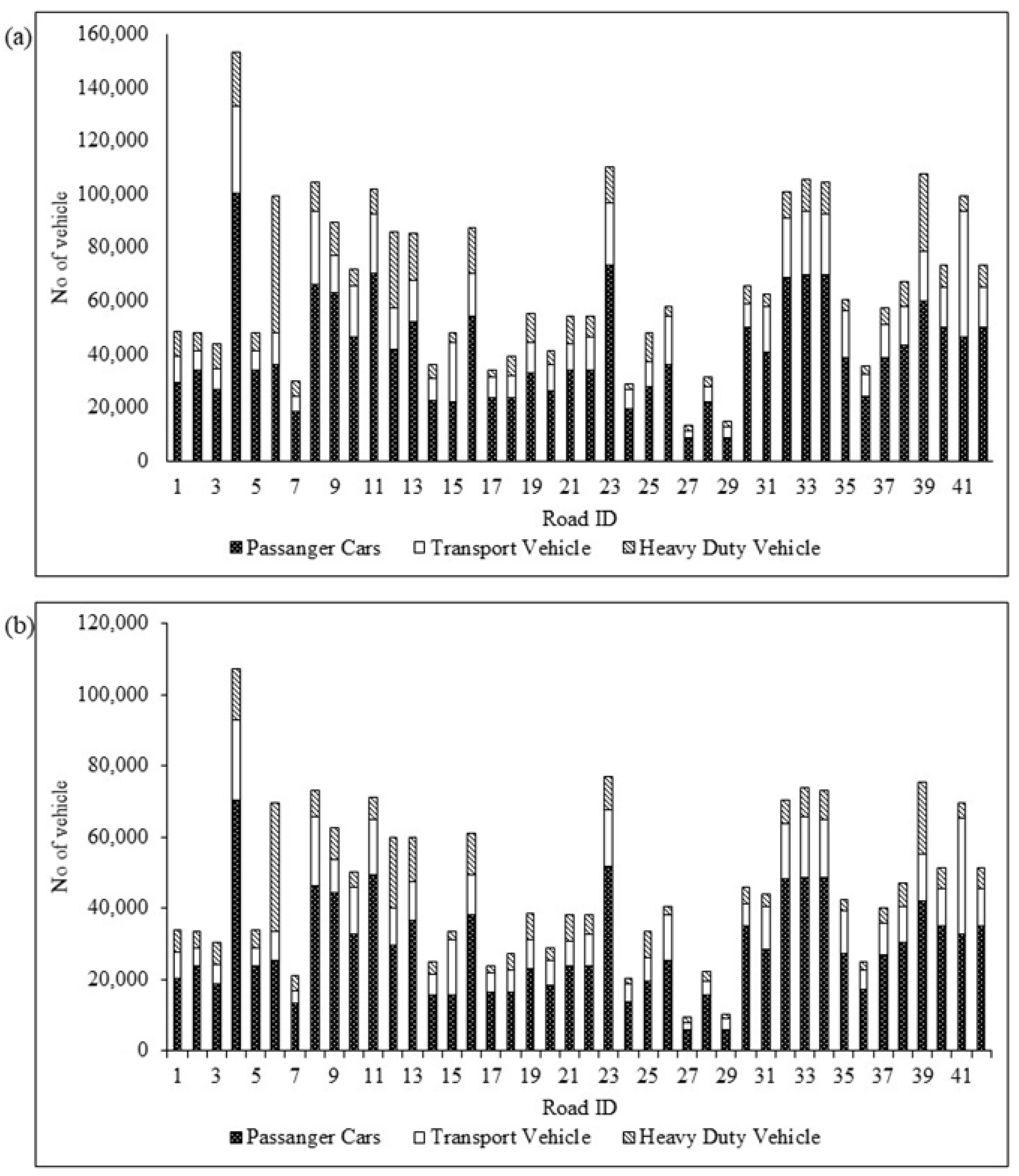
Figure 1. Location of Kuala Lumpur in Malaysian Peninsula; and location of target road in Kuala Lumpur City Center and Continuous Air Quality Monitoring Station (CAQMS) in Cheras, Kuala Lumpur.
Sustainability 13 05402 g001
Figure 2. A flowchart describing the research process and output of the study.
Sustainability 13 05402 g002
Figure 3. Annual average daily traffic (AADT) of the 41 selected target roads for (a) business as usual (b) 30% traffic reduction.
Sustainability 13 05402 g003
Figure 4. Comparison of the measured and modelled concentrations for (a) PM2.5 business as usual, (b) PM2.5 for 30% traffic reduction, (c) PM10 business as usual and (d) PM10 for 30% traffic reduction.
Sustainability 13 05402 g004
Figure 5. Spatial concentration map of annual mean for particulate matter in Kuala Lumpur City Centre for (a) business as usual (PM2.5), (b) 30% traffic reduction (PM2.5), (c) business as usual (PM10), and (d) 30% traffic reduction (PM10).
Sustainability 13 05402 g005
Figure 6. The diurnal concentration variation of (a) PM10 and (b) PM2.5 and from OML-Highway model prediction and CAQMS.
Sustainability 13 05402 g006
Figure 7. The weekly concentration variation of (a) PM10 and (b) PM2.5 and from OML-Highway model prediction and CAQMS.
Sustainability 13 05402 g007
Figure 8. The monthly concentration variation of (a) PM10 and (b) PM2.5 and from OML-Highway model prediction and CAQMS.
Sustainability 13 05402 g008
Table 1. Input data source and scenario for model run.
BAU Scenario30% Traffic Reduction Scenario
Road networkHighway and trunk road (DBKL, 2017)Highway and trunk road (DBKL, 2017)
Traffic dataTraffic data including number of vehicles for AADT, vehicle type, vehicle travel distance (km), vehicle speeds and activity (RTVM, 2019, DBKL, 2019)30% reduction of total traffic count from business as usual
Road typeHighway: Sultan Iskandar Highway, Ampang-Kuala Lumpur Elevated Highway, Sungai Besi Highway, Tun Razak Road
Mainroad: Bukit Bintang Road, Tun Tan Cheng Lock Road, DBP Road, Hang Tuah Road, Imbi Road, Kinabalu Road, Kuching Road, LTL Road, Loke Yew Road, Maharajalela Road, Melaka Road, Pahang Road, Parlimen Road, Pudu Road, Raja Laut Road, Raja Chulan Road, Raja Laut Road, RMAA Road, Sentul Road, Sultan Hishamuddin Road, Sultan Ismail Road, Kuching Road, TAR Road, Tun Ismail Road, Tun Perak Road, Tunku Road, Yew Road, Damansara Road
Average traffic speedHighway: 90 km/h
Mainroad: 60 km/h
Table 2. Comparison between average concentration of pollutants from site sampling and from OML-Highway model data (µg/m3).
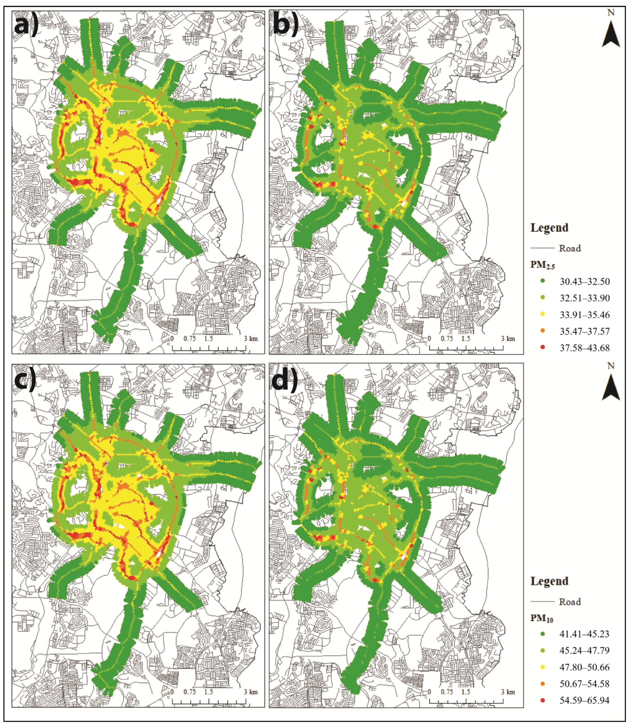
Concentration (Mean ± s.d.)
Model Data CAQMS
BAU Scenario30% Traffic Reduction Scenario
PM2.537.6 ± 24.335.3 ± 23.928.2 ± 22.2
PM1054.5 ± 27.850.76 ± 26.436.4 ± 24.2
Publisher’s Note: MDPI stays neutral with regard to jurisdictional claims in published maps and institutional affiliations.

