Examining the Impacts of the Built Environment on Quality of Life in Cancer Patients Using Machine Learning

Abstract

Despite accumulative evidence regarding the impact of the physical environment on health-related outcomes, very little is known about the relationships between built environment characteristics and the quality of life (QoL) of cancer patients. This study aims to investigate the association between the built environment and QoL by using survey data collected from cancer patients within the United States in 2019. To better understand the associations, we controlled the effects from sociodemographic attributes and health-related factors along with the residential built environment, including density, diversity, design, and distance to transit and hospitals on the self-reported QoL in cancer patients after treatment. Furthermore, machine learning models, i.e., logistic regression, decision tree, random forest, and multilayer perceptron neural network, were employed to evaluate the contribution of these features in predicting the QoL. The results from machine learning models indicated that the travel distance to the closest large hospital, perceived accessibility, distance to transit, and population density were among the most significant predictors of the cancer patients’ QoL. Additionally, the health insurance status, age, and education of patients are associated with QoL. The adverse effects of density on the self-reported QoL in this study can be addressed by individuals’ emotions towards negative aspects of density. Given the strong association between QoL and urban sustainability, consideration should be given to the side effects of urban density on cancer patients’ perceived wellbeing.

1. Introduction

The relationship between built environment and health-related conditions (such as physical activity, obesity, and cardiovascular disease) have been extensively discussed in previous studies [1,2,3]. Although the sustainable built environment is a multidimensional concept, the literature defines it through particular measures including the urban density and intensity of activities, diversity of land use, street network design, aesthetic qualities, and transportation facilities [4]. Neighborhood walkability, street connectivity, density, and mixed land use are associated with higher walking trips and physical activities [5,6,7] and can reduce the risk of cardiovascular disease [8,9]. Built environment attributes including density, diversity of land use, availability of destinations, and distance to transit can explain physical activity-related improvements in mortality and morbidity [10].

However, the evaluation of built environment attributes on cancer outcomes is a relatively novel arena that has not been extensively discussed in cancer-related research. Notably, a few studies discuss the role of residential neighborhoods on the level of physical activities and body mass of cancer patients [11,12,13,14], while a majority of literature focuses on the effects of geographical accessibility and distance to cancer care providers on cancer outcomes [15,16]. Meanwhile, some studies focus on the spatial cluster analysis of cancer-risk factors and suggest that the number of new cancer incidences is higher in metropolitan areas exposed to a high levels of air pollution when compared to less polluted geographical clusters [17].

The impact of built environment on primary and secondary cancer prevention can be investigated in four thematic areas of interest, including spatial proximity, transportation, land use, and housing [18]. Nonetheless, pioneer studies often concentrate on the spatial proximity and centralization of cancer care services in medical centers and large hospitals. This line of research investigates the travel burden to low-income and transit-oriented cancer patients dwelling in remote areas [19,20,21,22,23]. The previous studies often have utilized the neighborhood built environments to justify the health-related outcomes between different ethnicities (such as overweight and obesity) among cancer survivors [24,25] to mediate the relationships between the cancer risk and the socioeconomic status of the patients [14,24,25]. Access to neighborhood amenities such as recreational facilities, parks, and beaches have been demonstrated to contribute to the physical activity recommended by the American Cancer Society and improve cancer outcomes [14]. Moreover, a few scholars propose that population density has an influence on cancer mortality [14,15,26,27]. It seems that living in more densely populated neighborhoods is associated with higher risks of cancer incidents and poorer overall survival.

On the other hand, it is suggested that a supportive built environment can overcome the barriers in the outdoor environment and improve perceived quality of life (QoL) [28,29]. Notably, QoL, especially health-related QoL, denotes a broad-ranging concept with complex impacts related to physical health, psychological state, personal beliefs, social relationships, and a person’s relationship to salient features of their environment [30]. Analyzing cancer survivors indicates that micro-environmental conditions can affect their level of physical exercise and, consequently, the cancer patients’ quality of life [31]. Although evidence reveals that built environment characteristics promote physical activities, physical wellbeing, social interaction in the community, and mental health, the impacts of built environment on QoL is less recognized. Living in pedestrian-friendly neighborhoods with mixed-land use and well-designed green areas is associated with higher levels of self-reported wellbeing and mental health [32]. Examining the perceived neighborhood characteristics on health-related quality of life (HRQOL) reveals that perception of diversity, safety, and esthetics are associated with the higher physical and mental wellbeing of residents [33].

Contrary to the limited numbers of cancer studies investigating QoL and the built environment, several studies have been developed to understand how cancer experiences impact patients’ QoL as a multidimensional construct. Cancer types, pain intensity [34], and cancer treatment [35] have been identified as the most significant factors. Sociodemographic features and social supports, on the other hand, are also commonly considered as determinants of cancer patients’ QoL [36,37,38]. Evidence indicates that the QoL in cancer patients can be affected by race [39], age at diagnosis [40], access to health providers [41], and social support [42]. Some studies suggest that the association between the socioeconomic status of neighborhoods (such as race and ethnicity) and QoL result in health disparities in geographical areas [43]. It is deemed that performing physical activity such as walking and exercise interventions is significantly related to a higher QoL for patients with cancer history [44,45,46,47].

To the best of our knowledge, the impact of built environment attributes on cancer patients’ QoL has not been fully explored in the literature, and only a few studies have explored the relationships between neighborhood environments and QoL in urban settings [48]. Although little effort has been made to understand the effects of physical features such as access to goods and services on cancer survival through physical activities [14,25], the literature has not sufficiently explored the associations between built environment and QoL among the cancer patients. To our knowledge, these associations have not been investigated in the literature. Understanding the factors shaping patients’ QoL can help public health planners to recognize vulnerable groups of patients who require further support interventions and provide appropriate services to cancer survivors [49].

The growing need to develop sustainability in cities points to the importance of health and wellbeing in shaping sustainable communities. Researchers suggest a close association between QoL and environmental sustainability. Accordingly, in addition to measuring sustainability indicators, measuring and tracking the QoL of urban residents could be regarded as a critical goal of city planners and policymakers [50]. Moreover, the satisfaction of city residents regarding environmental sustainability indicators such as green spaces, air quality, noise level, cleanliness, and climate change can increase city livability and QoL [51]. Accordingly, investigating the effects of built environment factors on QoL can be regarded as an effort to understand the environmental sustainability concept.

This study aims to identify the factors that contribute to the QoL of people who struggle with cancer while considering a comprehensive set of internal and external factors. Accordingly, we address the following research questions: (1) How do built environment attributes along with health-related and sociodemographics shape the self-reporting QoL of cancer patients? and (2) What are the most influential factors associated with patients’ QoL?

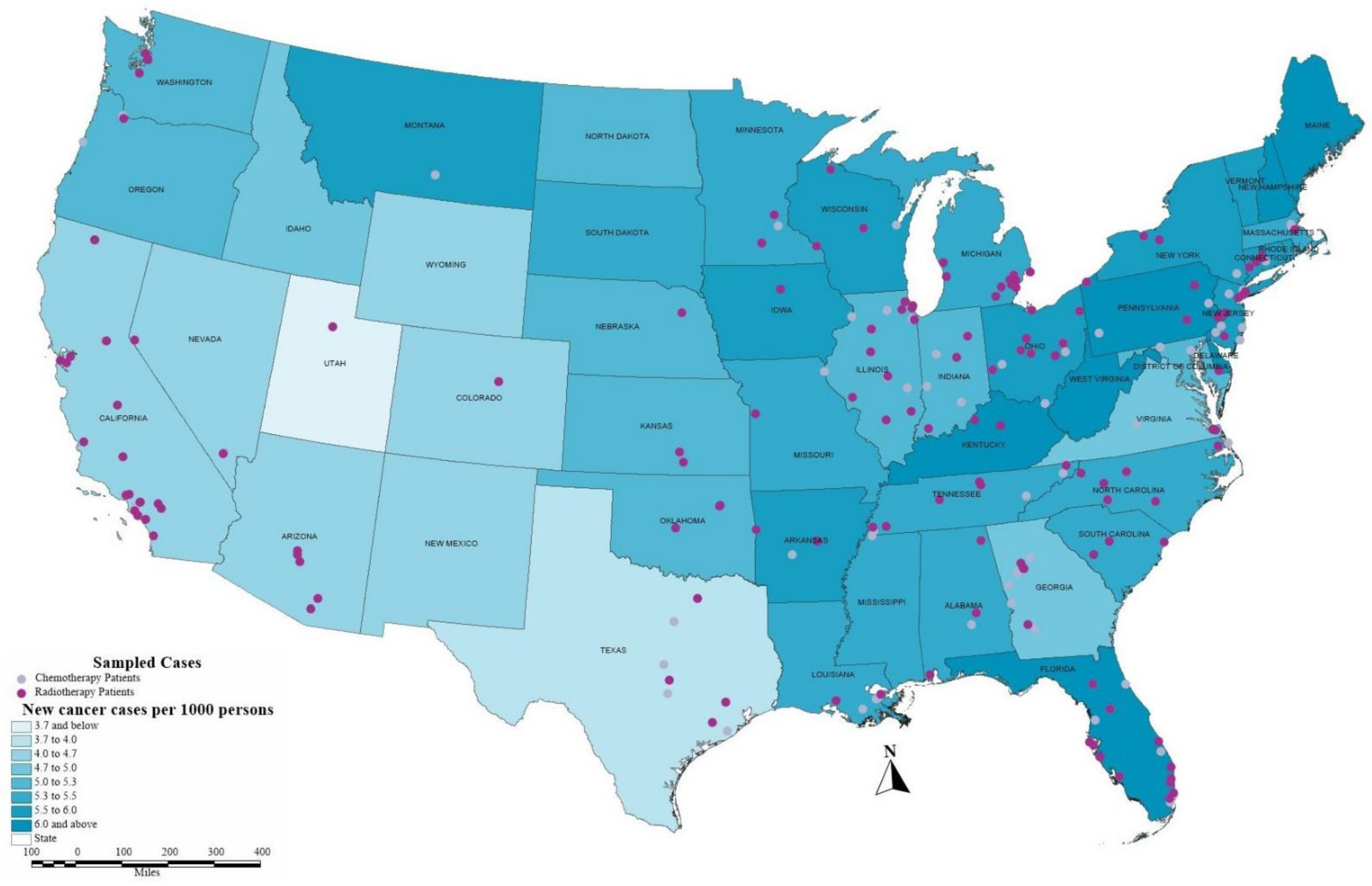
To fulfill the research gap, the present study designs a comprehensive survey to collect data from cancer patients across the US systematically. We explore the effects of built environment attributes by considering objective and actual measures as well as the subjective and perceptional factors. Furthermore, and to conduct a comprehensive framework, we employ the sociodemographic attributes and health-related variables suggested in the literature as the significant internal determinants of cancer patients’ QoL. Although most of the previous studies have focused on simple regression models to examine the linear relationship between QoL and its predictors [36,52], we employ machine learning models to analyze the survey data. The application of a broad conceptual model developed based on machine learning algorithms allows us to better understand self-reported QoL in cancer patients. Our study further incorporated machine learning models (i.e., logistic regression, decision tree, random forest, and multilayer perceptron neural network) to delineate the nonlinear patterns underlying the predictor variables with respect to the QoL of cancer patients. Results of this study have a great potential to help urban planners and policymakers design health-oriented neighborhoods that can improve cancer patients’ wellbeing and satisfaction.

2. Methods

2.1. Survey Data Collection and Pre-Processing

2.1.1. Survey Design

In this study, an online cross-sectional survey was designed to collect data from cancer patients across the US. All participants consented, and an Institutional Review Board (IRB) was approved for survey administration and data usage. To ensure the survey cohort, eligible participants must (1) have been treated by radiotherapy, chemotherapy, or other treatments, (2) be in remission or still seeking other treatments, and (3) be over 18 years old. The main objective of designing the questionnaire was to obtain information related to the behavioral patterns of the cancer patients during primary treatments including radiotherapy and chemotherapy, and other treatments. The questionnaire contained general information and questions related to the cancer type and the treatments, patients’ residential neighborhoods as well as their perceptions, attitudes, and quality of life. The third part of the questionnaire included the socioeconomic attributes of the respondents. After attaining the initial data (n = 950), we omitted those patients who filled in the questionnaires within less than 600 s to remove unreliable entries. To this end, a total number of 750 surveys remained for the spatial analysis.

2.1.2. Geocoding

By requesting the respondents’ home addresses, we geocoded home locations. We omitted cases with invalid home addresses that we were not able to locate on the map. The remaining addresses were fed into Google MyMap (https://www.caliper.com/maptovu.htm, accessed on 20 January 2020), which draws pushpins on locations corresponding to given addresses. To ensure every pushpin was located in the correct location, we manually verified each location by matching the home zip code and street names on Google maps with the address provided by the respondent. As such, we geocoded latitude and longitude coordinates of home address locations (n = 589). Figure 1 depicts the spatial disparities of the cancer patients according to the types of treatments (radiotherapy and chemotherapy).

2.1.3. Built Environment Measures

Earlier studies have often calculated the built environment attributes at census block level [53] or considering the zip codes of participants’ home addresses at the time of diagnosis [54]. While the literature has often measured the built environment at the block group level [14,24,25], this study measured the disaggregated built environment attributes in a one-mile buffer area around the participants’ home location. The built environment measures in the present study include density, land use diversity, street design, and distance to transit. Using a geographic information system (GIS), we joined different datasets to the extracted buffer layers and measured the built environment attributes.

To calculate population density, we used population data at the census tract level from the American Community Survey (ACS) (https://www.nhgis.org/, accessed on 6 February 2020). Hence, the population density of each participant’s home location was calculated within the corresponding one-mile buffer area.

Further, we computed an “entropy index” (EI) as our measure of land use diversity (mixed-use) in buffer areas [55]. The jobs by sectors, including five sectors that are known to be serving jobs (retail, services, food and accommodation, health, and education), were summed for blocks within the buffer areas of participants’ home locations. The entropy is calculated as follows:

$$EI=-\frac{\left({{\displaystyle \sum }}_{k=1}^K{P}_k\times \ln P_k\right)}{\ln K}$$

where P is the share of each of the five job sectors, and K is the number of sectors (i.e., K = 5). Notably, the EI ranges from 0 to 1, where the value of 1 shows the equal number of jobs in each of the sectors within the buffer area and 0 indicates that all jobs are in a single sector.

The distance to transit was measured according to the network distance from participants’ homes to the closest public transit stops by using Maptitude (https://www.caliper.com/maptovu.htm, accessed on 12 February 2020) software. Moreover, transit stop density was estimated by dividing the number of public transportations stops by the area of the buffers to evaluate the accessibility of the participants to public transportation. We measured the travel distance to the closest large hospital through the shortest travel time from the geocoded respondent’s home location. Travel distances of more than 50 miles were disregarded from the final analysis.

2.1.4. Perceived Built Environment and Accessibility

Although a supportive actual environment has been proven a necessary factor in improving individuals’ health outcomes, studies suggest the importance of the perceived environment in promoting active mobility and health-related behaviors [56]. To explore the perceived built environment, we asked the participants to evaluate their neighborhood’s characteristics on five-point Likert scales, where 1 = very poor to 5 = very good. Respondents stated how well their residence and its location met their needs through six statements in terms of easy access to their health provider, easy access to drugstores, closeness to work/school, closeness to family members, affordability of the neighborhood according to the patients’ income and their treatment costs, quietness, and safety and security of their neighborhood according to the cancer patients’ mental and physical condition. We then used confirmatory factor analysis (maximum likelihood with Promax rotation with 59.54% variance explained and Kaiser–Meyer–Olkin (KMO) = 0.869) to reduce the number of factors and extract one factor to indicate the perceived built environment. We also asked respondents to evaluate their residential accessibility in terms of approximate driving distance (in minutes) from their residential built environment to six different errands. We factor analyzed the distances to obtain a factor that indicated the built environment accessibility (maximum likelihood with Promax rotation with 62.27% variance explained and KMO = 0.879).

2.1.5. Quality of Life

All of our participants were selected from patients who had received three types of cancer treatments. Accordingly, to identify QoL, the survey included a self-reported question evaluating the respondents’ overall quality of life after cancer treatments in a five-point Likert type scale from 1 = terrible to 5 = excellent.

2.1.6. Other Key Variables

Previous studies have found that other key variables such as sociodemographic and health condition can also influence QoL. For instance, people on low income are more likely to have less physical activity and hence higher rates of morbidity and poorer physical function [57]. On the contrary, higher income adults are likely associated with higher levels of health-related QoL [58]. Accordingly, the survey contained self-reported questions related to the socioeconomic attributes of the patients including age, gender, income, race, education, employment status, homeownership, car ownership, and health insurance coverage.

Regarding cancer-related factors, the survey included questions about the cancer type and the type of treatments. We categorized the patients’ cancer types based on the diagnosis difficulty into three groups including easy, intermediate, and hard to diagnose [22]. Table 1 shows the descriptive statistics of the key variables and Table 2 demonstrates the results from the factor analysis. We also grouped the patient’s cancers based on radiotherapy and chemotherapy.

2.2. Predictive Modeling for Quality of Life of Cancer Patients

In the literature, machine learning models have been widely used for predictive modeling tasks, e.g., to predict chronic diseases and analysis of vital signs [59,60], to study the effects of built environment on driving distance [61], to identify abnormalities in manufacturing processes and schedule predictive maintenance [62,63,64], and to recognize transportation modes with mobile sensing [65,66]. In this study, four machine learning models, i.e., logistic regression, decision tree, random forest, and multilayer perceptron neural network, were employed to investigate how built environment characteristics, perceived built environment, socio-demographic attributes, and patients’ health-related variables were correlated with their QoL. Notably, the QoL scores are binarized into high- or low-level QoL using a cut-off QoL = 3. In other words, if a patient is with QoL ≥ 3, a label of “high-level of QoL” (i.e., 1), will be assigned. Otherwise, the patient will be associated with a label of “low-level of QoL” (i.e., 0). Let $\mathit{x}=\left(1,x_1,x_2,\dots ,x_m\right)$ denote the feature vector of an instance (i.e., a patient) and $y\in \left(0,1\right)$ be the label. In logistic regression, the log-odds for label 1 are calculated as:

$$\widehat{p}\left(\mathit{x}\right)=\frac{e^{{\beta }_0+{\beta }_1{x}_1+,\dots ,+{\beta }_m{x}_m}}{1+e^{{\beta }_0+{\beta }_1{x}_1+,\dots ,+{\beta }_m{x}_m}}=\frac{1}{1+e^{-\mathit{x}\mathit{\beta }}}$$

The parameter $\mathit{\beta }$ can be determined using the maximum likelihood estimation [67]. As a classification problem, we adopted 0.5 as the cut-off probability: if $\widehat{p}\left(\mathit{x}\right)\ge 0.5$, the estimated label $\widehat{y}$ was considered as 1. Otherwise, it was 0 [68].

The decision tree model deploys a tree-like structure to learn simple decision rules inferred from data. Starting from the root node, an instance is sorted through a sequence of internal nodes to reach a leaf node, which assigns a class label to the instance. Each internal node symbolizes a test on the instance and the path from the root to leaf node can be represented as a classification rule [69]. Assume the leaf node $h$ contains $n_h$ patients, we let

$${\widehat{p}}_{hk}=\frac{1}{n_h}{\displaystyle \sum }_{\mathit{x}\in R_h}I\left\{y=k\right\}$$

denote the proportion of class $k$ observations in node $h$. The patients in node $h$ can be classified based on majority voting:

$$k\left(h\right)=\arg \underset{k}{\max }{\widehat{p}}_{hk}$$

A few criteria can be used for splitting internal nodes, such as cross entropy and the Gini index [70]. Notably, although the decision tree method is considered a relatively simple approach, the generated classification rules are highly interpretable. Thus, it is still widely used in the machine learning community, especially among medical scientists [71].

An extension of the decision tree classifier is the random forest. It consists of a large number of decision trees that operate as an ensemble [72]. To ensure maximum diversity exists among the trees, the bootstrap aggregation (i.e., bagging) strategy is incorporated in the random forest [69]. That is, each decision tree is allowed to perform bootstrap (i.e., randomly sample from the dataset with replacement) and grow a decision tree based on the bootstrapped instances. Then, the prediction of class membership is based on a majority voting process. Let ${\widehat{y}}_t\left(\mathit{x}\right)$ be the predicted label from the $t\mathrm{th}$ decision tree for an instance with a feature vector $\mathit{x}$, meaning the final predicted label of that instance is:

$${\widehat{y}}_{forest}\left(\mathit{x}\right)=majorityvote{\left\{{\widehat{y}}_t\left(\mathit{x}\right)\right\}}_1^T$$

where $T$ is the total number of trees in the forest and this number can be adaptively tuned by the user [69]. Finally, a multilayer perceptron (MLP) neural network model was implemented. The MLP feature vectors in the input layer to the class labels in the output layer through hidden layers [73]. Usually, multiple hidden layers are incorporated to handle the nonlinearity of the input data. The output layer contains two neurons representing the classification results (i.e., 0 and 1) [74]. The mean squared normalized error is used as the performance measure of MLP and the weight associated with each neuron is optimized based on the backpropagation approach [75].

3. Results

3.1. Descriptive Statistics and Factor Analysis

Table 1. Characteristics of the study population (n = 589).

Variables	Description
		Count	Percent	Mean	S.D.
Socio-demographic attributes
Gender	Female	292	49.6
	Male	297	50.4
Race	White	510	86.6
	Non-white	79	13.4
Education	Well-educated (bachelor and above)	316	53.7
	Less-educated (below bachelor)	256	43.5
	Missing	17	2.9
Employment status	Employee	220	37.4
	Not-employee	364	61.8
	Missing	5	0.8
Residential status	Owner	219	37.2
	Not-owner	366	62.1
	Missing	4	0.7
Number of cars in the household	0	45	7.6
	1	243	41.3
	2	217	36.8
	3 or more	84	14.3
Health insurance	Medicaid	96	16.3
	Medicare	208	35.3
	Affordable Care Act	21	3.6
	Employer-paid insurance	142	24.1
	Private health insurance	54	9.2
	Uninsured	30	5.1
	Other insurance	37	6.3
	Missing	1	0.2
Income				50,872	28,132
Age				53	15.58
Household Size				2.55	1.36
Built environment characteristics
Population density				3714	6761
Entropy index				0.66	0.04
Intersection density				172	96
Transit stop density				12	20
Distance to transit (min)				27.29	95.23
Travel distance to the closest large hospital (min)				12	206
Perceptions
	Perceived built environment			99.72	25.33
	Perceived accessibility			92.99	15.16
Health-related variables
Cancer type (diagnosis)	Easy	285	48.4
	Intermediate	203	34.5
	Hard	72	12.2
	Unknown	29	4.9
Cancer treatments
Radiotherapy	1 = having radiotherapy	266	45.2
	0 = not having radiotherapy	323	54.8
Chemotherapy	1 = having chemotherapy	273	46.3
	0 = not having radiotherapy	316	53.7
Other	1 = having other treatment	261	44.3
	0 = not having radiotherapy	328	55.7
Quality of life
Overall quality of life	Terrible	17	2.9
	Poor	67	11.4
	Average	168	28.5
	Good	219	37.2
	Excellent	118	20

indicates that approximately half of the sample were male, with an average age of 53 years old. The majority of the cases were white American, mostly high-educated. The sample population was covered by a variety of health insurance, the majority of which are converged by Medicaid and Medicare. About 83% of the sample were categorized into the easy to intermediate levels of cancer diagnosis. As cancer patients can be treated by more than one type of treatment during the remedy, the sample can have multiple answers. Thus, the distribution of the three cancer treatments is slightly similar to each other.

Table 2. Results from the factor analysis for perceived built environment.

	Please Indicate How Well Your Residence and Its Location Meet the Following Characteristics	Loadings
Perceived built environment	Easy access to your health provider	0.788
	Easy access to drugstores	0.797
	Closeness to work/school	0.772
	Closeness to family members who can take care of me when I need them	0.730
	Affordable neighborhood according to income and treatment costs	0.805
	Quiet, safe, and secure neighborhood according to mental and physical condition	0.735
	Please indicate the approximate travel distance (in minutes) from your current residence to the following errands	Loadings
Perceived accessibility	Closest public transit station	0.517
	Closest gas station	0.846
	Closest restaurant/fast-food place	0.905
	Closest drugstore	0.896
	Closest grocery store	0.889
	Patients’ primary health provider	0.584

indicates the factor analysis for perceived accessibility and perceived built environment. Utilizing confirmatory factor analysis for each set of questions, we extracted two main factors.

3.2. Predictive Modeling Results

In this study, three metrics, i.e., accuracy, F-score, and area under the receiver operating characteristic curve (AUROC) were used for the evaluation of the performance of the proposed models. Accuracy was calculated as the correctly classified instances over the total number of instances. F-score balanced the precision and recall in the classification results. Precision referred to the number of true positives over predicted positive instances, whereas recall measured the ratio between the number of true positives and all positive instances [69]. AUROC calculated the area under the ROC curve, plotting the true positive rate versus the false positive rate. The true positive rate is the probability that a positive instance (i.e., a high QoL patient in our case) will be predicted as positive, and the false positive rate indicates the probability that a negative instance is considered as positive. Both the accuracy and F-score were in the range of (0,1) where the ideal value is 1. The AUROC ranged between 0.5 and 1, in which 0.5 corresponded to random classification and 1 corresponded to the perfect result. Notably, we randomly selected 80% of instances for training and 20% for test and each result is an average of 50 replications.

As shown in Figure 2, the most complex model, i.e., the MLP, achieved the highest accuracy for both the training (90%) and test sets (69%). Here, three hidden layers were deployed with 12, 12, and 6 neurons, respectively. The model with moderate complexity, e.g., the decision tree, achieved a test accuracy of 64%, which was slightly worse than the MLP but better than the logistic regression. Notably, the decision tree model is associated with high interpretability, and the obtained tree structure is visualized in Figure 3. In addition, the simplest model, i.e., logistic regression, achieved 66% and 61% accuracy for training and test, respectively. This corroborates the results from models with higher complexity and demonstrates the effectiveness of the selected predictive variables. Notably, the best accuracy for the test data achieved is ~70%. This is mainly due to the high heterogeneity of cancer patients within each group (i.e., high-level QoL and low-level QoL) as we binarized the continuous QoL scores from the survey.

In addition, the F-score and AUROC of each model are summarized in

Table 3. Performance results for various algorithms.

	Logistic Regression	Decision Tree	Random Forest	MLP
F-score	0.71	0.70	0.69	0.72
AUROC	0.64	0.67	0.63	0.66

. It is noteworthy that all four models achieved similar F-scores and AUROCs. The MLP achieved the best F-score, i.e., 0.72. The other three models, i.e., logistic regression, decision tree, and random forest, achieved slightly lower F-scores around 0.69 to 0.71. Further, the decision tree had the best AUROC, i.e., 0.67. The three other models obtained an AUROC ranging from 0.63 to 0.66. The results have shown that all the models are associate with good discriminative powers, and they are quite robust in predicting the patients in the positive class (i.e., patients with high QoL). This, in turn, indicates that our selected predictive variables are closely related to the QoL of cancer patients.

To gain insight into the usefulness of each feature, we computed the importance scores related to each feature considering the random forest approach. We omitted features with small scores and only considered the highest determinants of QoL (such as income, household size, perceived built environment).

Table 4. The most important features based on the random forest.

	Feature Name	Importance Score
1	Age	0.14198
2	Travel distance to closest large hospital	0.12031
3	Perceived accessibility	0.11206
4	Distance to transit (min)	0.10921
5	Population density	0.09243
6	Health insurance	0.08123
7	Entropy index	0.07142
8	Education (well-educated)	0.03246
9	Number of cars in the household	0.02834
10	Transit stop density	0.02341
11	Cancer treatments (chemotherapy)	0.02240
12	Employment status (employee)	0.01907
13	Cancer type (diagnosis)	0.01650
14	Gender	0.01106
15	Cancer treatments (radiotherapy)	0.00730
16	Race (white)	0.00659
17	Cancer treatments (other)	0.00292

indicates the top 17 features regarding the scores. The score is calculated as node impurity weighted by the probability of reaching that node and is normalized into (0,1). Moreover, to understand the relationship intensity and direction of the independent variables and QoL,

Table 5. Coefficient for each feature in the logistic regression model.

Variables	Coef	St. Error	Z	p-Values
Socio-demographic attributes
Gender (female)	0.2621	0.230	1.141	0.254
Race (white)	−0.0448	0.315	−0.142	0.887
Education (well-educated)	0.6215	00.213	2.922	0.003 ***
Employment status (employee)	0.2489	0.231	1.078	0.281
Number of cars in the household	0.2589	0.394	0.657	0.511
Health insurance	−0.7557	0.381	−1.984	0.047 ***
Age	1.8632	0.523	3.565	0.000 ***
Built environment characteristics
Population density	−14.1817	7.153	−1.983	0.047 ***
Entropy index	−0.2651	0.629	−0.421	0.673
Transit stop density	−0.4187	0.706	−0.593	0.553
Distance to transit (min)	−2.2074	1.367	−1. 614	0.106
Travel distance to closest large hospital	1.6386	1.127	1.453	0.146
Perceptions
Perceived accessibility	−1.1933	0.774	−1.543	0.123
Health-related variables
Cancer type (diagnosis)	0.1053	0.308	0.342	0.732
Cancer treatments (radiotherapy)	0.0180	0.251	0.072	0.943
Cancer treatments (chemotherapy)	−0.7943	0.263	−3.021	0.003 ***
Cancer treatments (other)	−0.3485	0.299	−1.164	0.244

*** indicates the significant p-value < 0.05.

summarizes the results from the logistic regression and describes the most significant determinants of QoL in cancer patients. The results from the logistic regression support the decision tree algorithms. Comparing Table 4 and Table 5 indicates that the top 10 features selected by random forest are with larger coefficients than other variables in the logistic regression model. However, the results from the decision tree effectively follow the scores of random forest and are relatively in line with the coefficients from the logistic model (see Figure 3). The age, health insurance, education, travel distance to the closest large hospital, and perceived accessibility are among the most important predictors of cancer patients’ QoL in both the decision tree and random forest scores.

4. Discussion

This study employs a cross-section survey to investigate how built environment impacts the quality of life (QoL) of cancer patients.

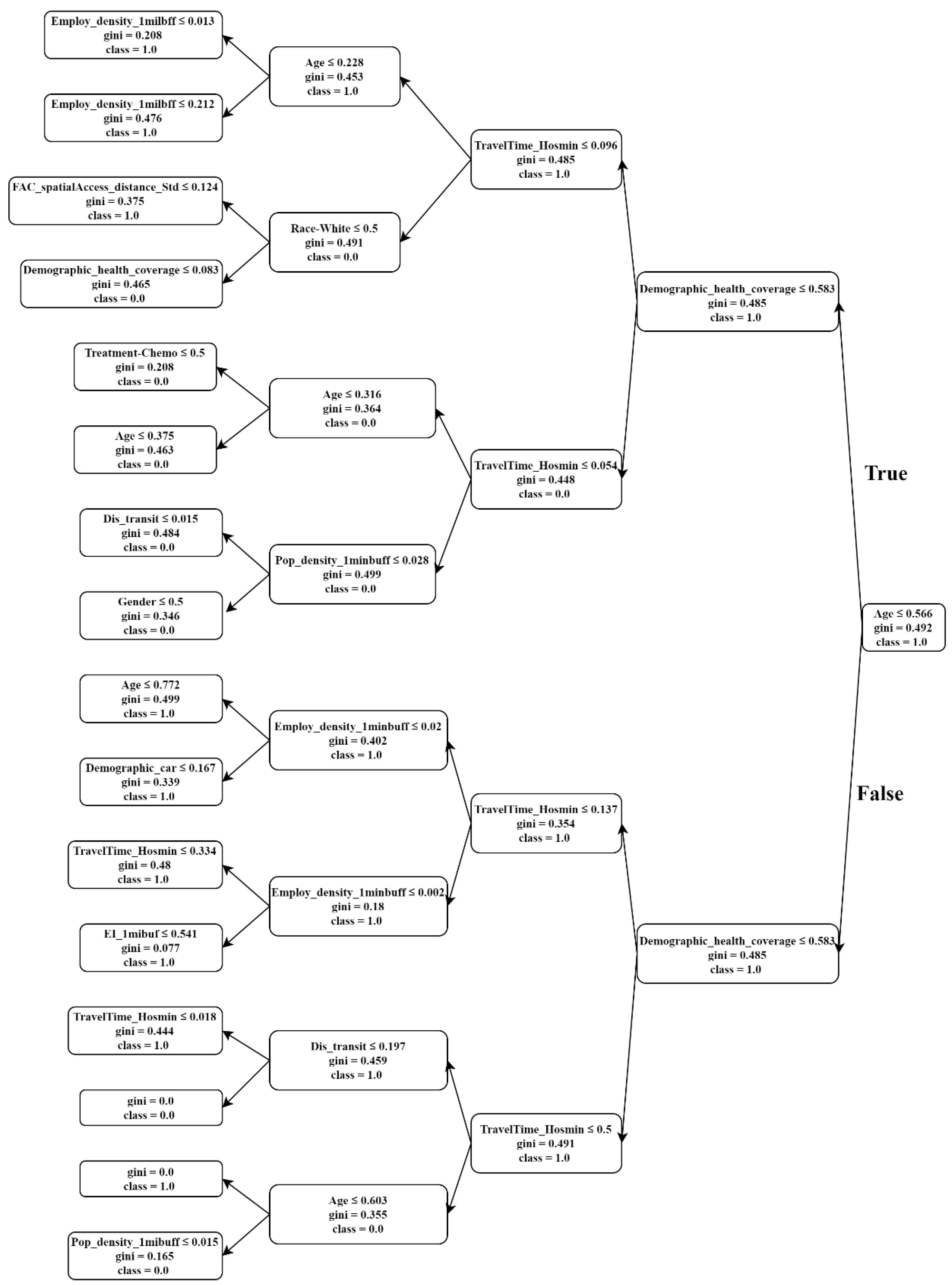
The random forest’s results demonstrate the top ten most important features that predict the QoL of cancer patients (Table 4) and the logistic regression indicates associations. Our results demonstrate that the built environment characteristics considerably contribute to predicting the QoL of the participants. According to the scored features in random forest, the travel distance to the closest hospital is one of the most significant predictors of QoL. Previous studies have suggested that the distance from residential neighborhoods to patients’ treating hospital influences cancer outcomes, and consequently, those who reside far from their care provides may have a lower QoL among cancer survivors [76]. Although travel distance to health facilities can be a barrier for cancer patients [77,78,79,80], this study considers the distance to the closest hospital and not the treated hospital. Hence, residing in neighborhoods distant from large hospital can be an indicator of living in the low-dense suburbs.

Perceived accessibility is the third predictor of the QoL in random forest [33]. The perception towards accessibility to the neighborhood local services such as access to schools, public transportation, medical care, and shopping exhibits a significant effect on self-rated health [81]. Although the logistic regression does not indicate a significant association between the perceived accessibility and QoL, it seems that patients residing with less accessibility (greater values of perceived accessibility), reported lower levels of QoL.

Distance to transit is the fourth important feature in the random forest. These measures are defined as the supportive built environment features that can significantly predict the QoL [29]. The literature introduces the distance to transit and residential density as two of the objective indicators measuring the quality of urban life [50]. According to the logistic model, patients residing in areas with more distance to transit declare lower QoL. The association is not statistically significant, but the direction is aligned with the theory.

Population density is another determinant of QoL in the random forest. Despite the lack of a clear understanding of the mechanism under which different urban densities influence QoL, some studies have suggested that high density positively affects life satisfaction [82]. Higher population density can be positively associated with subjective wellbeing when accompanied by mixed land uses, public transport, limited car traffic, access to green spaces, and social equity [83]. People who reside in higher density neighborhoods are more likely to perform physical activities [84] and more able to experience better health conditions and life satisfaction [85]. On the other hand, some research suggests that living in less dense areas can increase the quality of life while controlling for all the other sociodemographic and somatic health variables [86]. Accordingly, urban density contributes to QoL in different ways. The results of logistic regression in terms of density and QoL associations indicates an evident paradox. Earlier studies have often reported a positive relationship between population density and health outcomes due to the availability of walkable destinations, and consequently a higher tendency towards walking, biking, or public transit [87,88]. In contrast, our results suggest that a higher level of QoL is reported by participants in neighborhoods with lower population density. Research on compact city form states that the negative association between life satisfaction and urban density stems from the emotional response of the residents toward perceived crime and stress in crowded and noisy neighborhoods [83]. In contrast, residing in low-dense suburbs has positive effects on the wellbeing of individuals through positive emotions and calmness [89]. In addition, higher levels of anxiety can be found in high-density areas and consequently decrease mental health [90]. The positive effects of density on wellbeing occur when it brings with it mixed land use, access to public transit, restricted car travel, access to green spaces, and social equity [83]. Accordingly, the adverse effects of population density on the self-reported QoL in cancer patients can be a result of their negative emotions towards the negative aspects of density, such as traffic congestion, the sense of crime, and lack of green space.

The scored features of the random forest reveal that the entropy index plays a moderate role in defining the level of self-reported QoL in cancer patients. Neighborhoods with mixed land use provide the cancer survivors accessibility to different errands in a walkable distance [25]. This result is in accordance with some previous studies about the compact city form in which mixed land use has the potential to provide a better quality of life through offering longer, healthier, and safer lives and contributing to the economic wellbeing and health of cities [91].

Random forest scores show that among all sociodemographic characteristics, respondents’ age has an enormous contribution to the level of QoL among cancer patients. It seems that the process of aging in cancer patients can influence disease adjustment and therefore impact the health-related QoL [92]. Our results from the regression model reveal that older cancer patients have a higher level of QoL. This finding is in line with similar studies, which suggest that younger patients feel worse than older adults on some quality of life dimensions because they suffer more from psychological symptoms and financial issues [93,94].

The random forest score of health insurance shows that this feature can differentiate the QoL experience through different levels. This result is in line with previous studies that demonstrate health insurance status is associated with health-related attributes of cancer patients over time [95]. Since patients with poorer insurance coverage may have less access to high-quality treatment, this can result in later diagnoses and worse outcomes [96]. This result confirms empirical evidence, which shows that health insurance can reinforce the health of vulnerable groups, such as senior adults, children, and people with premedical conditions and low-income populations [97]. Moreover, the associations between health insurance and QoL explain that participants who have private and/or employer-paid insurance health insurance reported a higher QoL levels compared with low-income participants who have government-related insurance. It confirms previous studies that report that cancer-related financial burdens are related to an increased risk of depression and lower health-related QoL levels in cancer patients [98].

The number of cars in the family is the tenth significant factor in predicting the QoL that has been identified by the random forest. To the best of our knowledge, there is no evidence to identify the effect of vehicle ownership on the QoL of cancer patients. However, the vehicle is the most usual mobility mode particularly for residents of distant and rural areas, so, it can affect a cancer patients’ access to treatment facilities where they might not have access to other mobility modes [77,78,99,100]. Access to private vehicles and the option of driving with others are among the most crucial treatment-related factors that impose barriers to cancer patients [101]. Vehicle availability is assumed as a variable that has a positive relationship with the early diagnosis stage [15] and receiving the first line of treatments [79]. Patients residing in areas having no access to a private vehicle are less likely to follow cancer screening treatments [102]. This evidence can support the contribution of access to a car in the QoL of cancer patients.

Furthermore, education is another factor contributing to the QoL of cancer patients. This result supports the studies that propose education improves wellbeing because it develops access to economic devices, enhances a person’s sense of control over life, and increases social support [103]. The positive association between education and QoL in this study can be justified by the earlier research suggesting that low education along with low neighborhood socioeconomic status result in worse all-kind survival for particular cancers [24]. The higher score related to the significance of chemotherapy compared with radiotherapy reveals that chemotherapy treatment has a more significant contribution in predicting quality of life [104]. Chemotherapy treatment appears to have a negative effect on the QoL of patients who received this treatment. Although physicians suggest chemotherapy to improve QoL for patients with end-stage cancer, it cannot reinforce QoL for patients with moderate or poor performance status and worsened QoL close for patients with good performance status [105]. Gender and race have a small participation in determining the level of QoL. The race of the participants (white versus other races) has a small but notable effect on QoL after treatment [106].

5. Conclusions

This study brings new insights regarding the impacts of actual and perceived built environment characteristics on the QoL of cancer patients while controlling sociodemographic and health-related factors. To address the first research question regarding the factors explaining the self-reporting QoL, we employed the random forest approach. Results suggested that the QoL of cancer patients can be principally influenced by built environment features, including travel distance to a closest large hospital, perceived accessibility, distance to transit, population density, and sociodemographic factors such as age, health insurance status, and education. Results from the logistic regression fulfill the second research question regarding the most significant determinants of QoL in cancer patients. Population density, age, education, health insurance, and chemotherapy treatment are the most critical determinants of QoL in cancer patients. We point out the main research outcomes in the following areas:

• Our findings regarding the effects of built environment features such as density and access to healthcare facilities on the QoL of cancer patients indicate that a supportive built environment can overcome the barriers in the outdoor environment, increase the likelihood of physical activity, and therefore improve perceived quality of life. These results point out that urban design and transportation planning need to become more friendly for this population group with particular needs and requirements.
• To improve social equity, it is fundamental to design environments compatible with the needs of all community groups, including people who are struggling with chronic diseases that require ongoing medical attention or limit activities of daily living in the long term.
• Understanding the associations between built environment and health-related QoL can help in the development of intervention policies that aim to improve cancer patients’ wellbeing. Hence, there is a need for collaboration between transit agencies, MPOs, and community planners to target the living environment and mobility needs of people who are burdened with chronic disease. To this end, urban and transportation planners and practitioners should be more involved in this field and acquire more knowledge from other disciplines. Integrating transportation planning with public health and social studies could reinforce existing policies and strategies in transportation accessibility and equity and therefore increase wellbeing and QoL.
• In addition, there is an inherent need to develop a QoL measurement that comprehensively counts for subjective feelings as well as objective factors in terms of patients’ health condition, transportation, and built environment. This QoL measurement can be used as a policy tool by communities and local governments to evaluate the extent to which the mobility and built environment meet the needs of patients with chronic diseases.
• The inverse associations between population density and cancer patients’ QoL indicate that compact development strategies can be fulfilled when policymakers address the side effects of urban density, such as fear of crime, high noise, and traffic congestion. This compact development pattern should concentrate on strategies that increase robust transportation options and improve public health indicators such as air quality while creating safe and secure neighborhoods that preserve more open space.

There is large room for improvement in our understanding of the effects of built environment and transportation accessibility on cancer patients’ QoL in future research. Working with the small sample size in our study can be a principal limitation of our study, which may have caused some failures in identifying more associations between the key variables, particularly in the logistic regression model. Further studies need to be developed to collect data on a large population of cancer patients regarding their mobility needs, their concerns towards residential neighborhoods, and their preferences about the attributes of a supportive neighborhood that can overcome their physical, mental, social, and environmental barriers. The other limitation of this study is related to measuring QoL. Measuring the QoL of the patients through standard EQ-5D-5L or Q-5D-3L criteria can allow future studies to explain the QoL of cancer patients thoroughly. This study also emphasizes the need for collaboration between health policymakers, urban planners, and transportation experts to conduct more research regarding the effects of transportation policies on health outcomes.

References

1. Sallis, J.F.; Floyd, M.F.; Rodríguez, D.A.; Saelens, B.E. Role of Built Environments in Physical Activity, Obesity, and Cardiovascular Disease. Circulation 2012, 125, 729–737. [Google Scholar] [CrossRef]
2. Saelens, B.E.; Handy, S.L. Built Environment Correlates of Walking: A Review. Med. Sci. Sports Exerc. 2008, 40 (Suppl. 7), S550–S566. [Google Scholar] [CrossRef] [Green Version]
3. Brownson, R.C.; Hoehner, C.M.; Day, K.; Forsyth, A.; Sallis, J.F. Measuring the Built Environment for Physical Activity. Am. J. Prev. Med. 2009, 36, S99–S123.e12. [Google Scholar] [CrossRef] [Green Version]
4. Handy, S.L.; Boarnet, M.G.; Ewing, R.; Killingsworth, R.E. How the built environment affects physical activity. Am. J. Prev. Med. 2002, 23, 64–73. [Google Scholar] [CrossRef]
5. Van, H.V.; Deforche, B.; Van, C.J.; Goubert, L.; Maes, L.; Van de Weghe, N.; De Bourdeaudhuij, I. Relationship between the physical environment and different domains of physical activity in European adults: A systematic review. BMC Public Health 2012, 12, 807. [Google Scholar]
6. Duncan, M. Would the replacement of park-and-ride facilities with transit-oriented development reduce vehicle kilometers traveled in an auto-oriented US region? Transp. Policy 2017, 81, 293–301. [Google Scholar] [CrossRef]
7. Ewing, R.; Cervero, R. Travel and the Built Environment: A Meta-Analysis. J. Am. Plan. Assoc. 2010, 76, 265–294. [Google Scholar] [CrossRef]
8. Lovasi, G.S.; Grady, S.; Rundle, A. Steps forward: Review and recommendations for research on walkability, physical activity and cardiovascular health. Public Health Rev. 2011, 33, 484. [Google Scholar] [CrossRef] [Green Version]
9. Leal, C.; Chaix, B. The influence of geographic life environments on cardiometabolic risk factors: A systematic review, a methodological assessment and a research agenda. Obes. Rev. 2011, 12, 217–230. [Google Scholar] [CrossRef]
10. Zapata-Diomedi, B.; Herrera, A.M.M.; Veerman, J.L. The effects of built environment attributes on physical activity-related health and health care costs outcomes in Australia. Health Place 2016, 42, 19–29. [Google Scholar] [CrossRef] [Green Version]
11. Lynch, B.M.; Owen, N.; Hawkes, A.L.; Aitken, J.F. Perceived barriers to physical activity for colorectal cancer survivors. Support Care Cancer 2010, 18, 729–734. [Google Scholar] [CrossRef]
12. Schootman, M.; Deshpande, A.D.; Pruitt, S.L.; Jeffe, D.B. Neighborhood foreclosures and self-rated health among breast cancer survivors. Qual. Life Res. 2012, 21, 133–141. [Google Scholar] [CrossRef] [PubMed] [Green Version]
13. Pruitt, S.L.; McQueen, A.; Deshpande, A.D.; Jeffe, D.B.; Schootman, M. Mediators of the effect of neighborhood poverty on physical functioning among breast cancer survivors: A longitudinal study. Cancer Causes Control 2012, 23, 1529–1540. [Google Scholar] [CrossRef]
14. Keegan, T.H.M.; Shariff-Marco, S.; Sangaramoorthy, M.; Koo, J.; Hertz, A.; Schupp, C.W.; Yang, J.; John, E.M.; Gomez, S.L. Neighborhood influences on recreational physical activity and survival after breast cancer. Cancer Causes Control 2014, 25, 1295–1308. [Google Scholar] [CrossRef] [Green Version]
15. Parsons, M.A.; Askland, K.D. Determinants of prostate cancer stage in northern New England: USA Franco-American contextual effects. Soc. Sci. Med. 2007, 65, 2018–2030. [Google Scholar] [CrossRef]
16. Russell, E.; Kramer, M.R.; Cooper, H.L.F.; Thompson, W.W.; Arriola, K.R.J. Residential Racial Composition, Spatial Access to Care, and Breast Cancer Mortality among Women in Georgia. J. Urban Health 2011, 88, 1117–1129. [Google Scholar] [CrossRef] [PubMed] [Green Version]
17. Majcherek, D.; Weresa, M.A.; Ciecierski, C. Understanding Regional Risk Factors for Cancer: A Cluster Analysis of Lifestyle, Environment and Socio-Economic Status in Poland. Sustainability 2020, 12, 9080. [Google Scholar] [CrossRef]
18. Wray, A.J.D.; Minaker, L.M. Is cancer prevention influenced by the built environment? A multidisciplinary scoping review. Cancer 2019, 125, 3299–3311. [Google Scholar] [CrossRef]
19. Pitchforth, E.; Russell, E.; Van der Pol, M. Access to specialist cancer care: Is it equitable? Br. J. Cancer 2002, 87, 1221–1226. [Google Scholar] [CrossRef]
20. Jordan, H. The Index of Multiple Deprivation 2000 and accessibility effects on health. J. Epidemiol. Community Health 2004, 58, 250–257. [Google Scholar] [CrossRef]
21. Campbell, N.C.; Elliott, A.M.; Sharp, L.; Ritchie, L.D.; Cassidy, J.; Little, J. Rural and urban differences in stage at diagnosis of colorectal and lung cancers. Br. J. Cancer 2001, 84, 910–914. [Google Scholar] [CrossRef] [Green Version]
22. Flytkjær Virgilsen, L.; Møller, H.; Vedsted, P. Cancer diagnostic delays and travel distance to health services: A nationwide cohort study in Denmark. Cancer Epidemiol. 2019, 59, 115–122. [Google Scholar] [CrossRef]
23. Ringstrom, M.J.; Christian, J.; Bush, M.L.; Levy, J.E.; Huang, B.; Gal, T.J. Travel distance: Impact on stage of presentation and treatment choices in head and neck cancer. Am. J. Otolaryngol. 2018, 39, 575–581. [Google Scholar] [CrossRef] [PubMed]
24. Shariff-Marco, S.; Von Behren, J.; Reynolds, P.; Keegan, T.H.M.; Hertz, A.; Kwan, M.L.; Roh, J.M.; Thomsen, C.; Kroenke, C.H.; Ambrosone, C.; et al. Impact of Social and Built Environment Factors on Body Size among Breast Cancer Survivors: The Pathways Study. Cancer Epidemiol. Biomark. Prev. 2017, 26, 505–515. [Google Scholar] [CrossRef] [Green Version]
25. Conroy, S.M.; Shariff-Marco, S.; Koo, J.; Yang, J.; Keegan, T.H.M.; Sangaramoorthy, M.; Hertz, A.; Nelson, D.O.; Cockburn, M.; Satariano, W.A.; et al. Racial/Ethnic Differences in the Impact of Neighborhood Social and Built Environment on Breast Cancer Risk: The Neighborhoods and Breast Cancer Study. Cancer Epidemiol. Biomark. Prev. 2017, 26, 541–552. [Google Scholar] [CrossRef] [Green Version]
26. Chaix, B.; Rosvall, M.; Lynch, J.; Merlo, J. Disentangling contextual effects on cause-specific mortality in a longitudinal 23-year follow-up study: Impact of population density or socioeconomic environment? Int. J. Epidemiol. 2006, 35, 633–643. [Google Scholar] [CrossRef]
27. Freedman, V.A.; Grafova, I.B.; Rogowski, J. Neighborhoods and Chronic Disease Onset in Later Life. Am. J. Public Health 2011, 101, 79–86. [Google Scholar] [CrossRef]
28. Rantakokko, M.; Iwarsson, S.; Kauppinen, M.; Leinonen, R.; Heikkinen, E.; Rantanen, T. Quality of Life and Barriers in the Urban Outdoor Environment in Old Age: Quality of Life and Outdoor Environment. J. Am. Geriatr. Soc. 2010, 58, 2154–2159. [Google Scholar] [CrossRef]
29. Engel, L.; Chudyk, A.M.; Ashe, M.C.; McKay, H.A.; Whitehurst, D.G.T.; Bryan, S. Older adults’ quality of life–Exploring the role of the built environment and social cohesion in community-dwelling seniors on low income. Soc. Sci. Med. 2016, 164, 1–11. [Google Scholar] [CrossRef]
30. WHOQOL. Measuring Quality of Life: The World Health Organization Quality of Life Instruments (the WHOQOL-100 and the WHOQOL-BRIEF); Division of Mental Health and Prevention of Substance Abuse: Geneva, Switzerland, 1997. [Google Scholar]
31. Fonseca, V.; Caeiro, J.; Nogueira, F. Social Model—Innovation and Behavioural Intervention as a Public Policy of Action within an Oncology and Loneliness Scope. Sustainability 2021, 13, 1544. [Google Scholar] [CrossRef]
32. Kim, D.; Subramanian, S.V.; Kawachi, I. Social capital and physical health. In Social Capital and Health; Springer: Berlin/Heidelberg, Germany, 2008; pp. 139–190. [Google Scholar]
33. Gao, M.; Ahern, J.; Koshland, C.P. Perceived built environment and health-related quality of life in four types of neighborhoods in Xi’an, China. Health Place 2016, 39, 110–115. [Google Scholar] [CrossRef] [PubMed]
34. Heydarnejad, M.S.; Hassanpour, D.A.; Solati, D.K. Factors affecting quality of life in cancer patients undergoing chemotherapy. Afr. Health Sci. 2011, 11, 266–270. [Google Scholar] [PubMed]
35. Payne, R.; Mathias, S.D.; Pasta, D.J.; Wanke, L.A.; Williams, R.; Mahmoud, R. Quality of life and cancer pain: Satisfaction and side effects with transdermal fentanyl versus oral morphine. J. Clin. Oncol. 1998, 16, 1588–1593. [Google Scholar] [CrossRef] [PubMed]
36. Parker, P.A.; Baile, W.F.; de Moor, C.; Cohen, L. Psychosocial and demographic predictors of quality of life in a large sample of cancer patients. Psychooncology 2003, 12, 183–193. [Google Scholar] [CrossRef]
37. Costa, A.L.S.; Heitkemper, M.M.; Alencar, G.P.; Damiani, L.P.; da Silva, R.M.; Jarrett, M.E. Social support is a predictor of lower stress and higher quality of life and resilience in Brazilian patients with colorectal cancer. Cancer Nurs. 2017, 40, 352–360. [Google Scholar] [CrossRef]
38. Astrup, G.L.; Rustøen, T.; Hofsø, K.; Gran, J.M.; Bjordal, K. Symptom burden and patient characteristics: Association with quality of life in patients with head and neck cancer undergoing radiotherapy. Head Neck 2017, 39, 2114–2126. [Google Scholar] [CrossRef]
39. Sarna, L.; Padilla, G.; Holmes, C.; Tashkin, D.; Brecht, M.L.; Evangelista, L. Quality of life of long-term survivors of non–small-cell lung cancer. J. Clin. Oncol. 2002, 20, 2920–2929. [Google Scholar] [CrossRef]
40. Cimprich, B.; Ronis, D.L.; Martinez-Ramos, G. Age at Diagnosis and Quality of Life in Breast Cancer Survivors. Cancer Pract. 2002, 10, 85–93. [Google Scholar] [CrossRef] [PubMed]
41. Drury, A.; Payne, S.; Brady, A.-M. Identifying associations between quality of life outcomes and healthcare-related variables among colorectal cancer survivors: A cross-sectional survey study. Int. J. Nurs. Stud. 2020, 101, 103434. [Google Scholar] [CrossRef]
42. Wenzel, L.; DeAlba, I.; Habbal, R.; Kluhsman, B.C.; Fairclough, D.; Krebs, L.U.; Anton-Culver, H.; Berkowitz, R.; Aziz, N. Quality of life in long-term cervical cancer survivors. Gynecol. Oncol. 2005, 97, 310–317. [Google Scholar] [CrossRef] [Green Version]
43. Green, C.; Hart-Johnson, T. Neighborhood SES and chronic pain: Impact on quality of life of cancer survivors. J. Pain. 2011, 12, 84. [Google Scholar] [CrossRef]
44. Oh, Y.J.; Kim, C.-M.; Lee, Y.J.; Yoon, J.; Kim, M.S.; Kim, S.J.; Shin, H.H. Predictive Factors for Quality of Life and Impact of Physical Activity in Korean Breast Cancer Survivors. Korean J. Fam. Pract. 2018, 8, 380–385. [Google Scholar] [CrossRef]
45. Mishra, S.I.; Scherer, R.W.; Geigle, P.M.; Berlanstein, D.R.; Topaloglu, O.; Gotay, C.C. Exercise Interventions on Health-Related Quality of Life for Cancer Survivors; Cochrane Gynaecological, Neuro-Oncology and Orphan Cancer Group, Ed.; Cochrane Database of Systematic Reviews; Wiley: Hoboken, NJ, USA, 2012; Available online: http://0-doi-wiley-com.brum.beds.ac.uk/10.1002/14651858.CD007566.pub2 (accessed on 17 April 2020).
46. Ho, K.Y.; Li, W.H.C.; Lam, K.W.K.; Wei, X.; Chiu, S.Y.; Chan, C.-F.G.; Chung, O.K.J. Relationships among fatigue, physical activity, depressive symptoms, and quality of life in Chinese children and adolescents surviving cancer. Eur. J. Oncol. Nurs. 2019, 38, 21–27. [Google Scholar] [CrossRef] [PubMed] [Green Version]
47. Gopalakrishna, A.; Longo, T.A.; Fantony, J.J.; Harrison, M.R.; Inman, B.A. Physical activity patterns and associations with health-related quality of life in bladder cancer survivors. Urol. Oncol. Semin. Orig. Investig. 2017, 35, 540.e1–540.e6. [Google Scholar] [CrossRef] [PubMed]
48. Schootman, M.; Perez, M.; Schootman, J.C.; Fu, Q.; McVay, A.; Margenthaler, J.; Colditz, G.A.; Kreuter, M.W.; Jeffe, D.B. Influence of built environment on quality of life changes in African-American patients with non-metastatic breast cancer. Health Place 2020, 63, 102333. [Google Scholar] [CrossRef] [PubMed]
49. Zebrack, B.J. Cancer Survivor Identity and Quality of Life. Cancer Pract. 2000, 8, 238–242. [Google Scholar] [CrossRef]
50. Marans, R.W. Quality of urban life & environmental sustainability studies: Future linkage opportunities. Habitat Int. 2015, 45, 47–52. [Google Scholar]
51. Del Mar Martínez-Bravo, M.; Martínez-del-Río, J.; Antolín-López, R. Trade-offs among urban sustainability, pollution and livability in European cities. J. Clean. Prod. 2019, 224, 651–660. [Google Scholar] [CrossRef]
52. Nipp, R.D.; El-Jawahri, A.; Fishbein, J.N.; Eusebio, J.; Stagl, J.M.; Gallagher, E.R.; Park, E.R.; Jackson, V.A.; Pirl, W.F.; Greer, J.A.; et al. The relationship between coping strategies, quality of life, and mood in patients with incurable cancer: Coping in Patients with Incurable Cancer. Cancer 2016, 122, 2110–2116. [Google Scholar] [CrossRef]
53. Vieira, V.M.; Villanueva, C.; Chang, J.; Ziogas, A.; Bristow, R.E. Impact of community disadvantage and air pollution burden on geographic disparities of ovarian cancer survival in California. Environ. Res. 2017, 156, 388–393. [Google Scholar] [CrossRef]
54. Robert, S.A.; Strombom, I.; Trentham-Dietz, A.; Hampton, J.M.; McElroy, J.A.; Newcomb, P.A.; Remington, P.L. Socioeconomic risk factors for breast cancer: Distinguishing individual-and community-level effects. Epidemiology 2004, 15, 442–450. [Google Scholar] [CrossRef] [PubMed]
55. Hamidi, S.; Ewing, R. A longitudinal study of changes in urban sprawl between 2000 and 2010 in the United States. Landsc. Urban Plan. 2014, 128, 72–82. [Google Scholar] [CrossRef]
56. Ma, L.; Dill, J. Associations between the objective and perceived built environment and bicycling for transportation. J. Transp. Health 2015, 2, 248–255. [Google Scholar] [CrossRef]
57. Nilsson, C.J.; Avlund, K.; Lund, R. Social Inequality in Onset of Mobility Disability among Older Danes: The Mediation Effect of Social Relations. J. Aging Health 2010, 22, 522–541. [Google Scholar] [CrossRef]
58. Sallis, J.F.; Saelens, B.E.; Frank, L.D.; Conway, T.L.; Slymen, D.J.; Cain, K.L.; Chapman, J.E.; Kerr, J. Neighborhood built environment and income: Examining multiple health outcomes. Soc. Sci. Med. 2009, 68, 1285–1293. [Google Scholar] [CrossRef] [Green Version]
59. Chen, M.; Hao, Y.; Hwang, K.; Wang, L.; Wang, L. Disease Prediction by Machine Learning Over Big Data from Healthcare Communities. IEEE Access 2017, 5, 8869–8879. [Google Scholar] [CrossRef]
60. Charleonnan, A.; Fufaung, T.; Niyomwong, T.; Chokchueypattanakit, W.; Suwannawach, S.; Ninchawee, N. Predictive analytics for chronic kidney disease using machine learning techniques. In Proceedings of the 2016 Management and Innovation Technology International Conference (MITicon), Bang-San, Thailand, 12–14 October 2016; pp. MIT-80–MIT-83. [Google Scholar]
61. Ding, C.; Cao, X.; Næss, P. Applying gradient boosting decision trees to examine non-linear effects of the built environment on driving distance in Oslo. Transp. Res. Part A Policy Pract. 2018, 110, 107–117. [Google Scholar] [CrossRef]
62. Liu, J.; Zhang, Z.; Razavian, N. Deep EHR: Chronic Disease Prediction Using Medical Notes. arXiv 2018, arXiv:180804928. Available online: http://arxiv.org/abs/1808.04928 (accessed on 25 October 2020).
63. Kan, C.; Yang, H.; Kumara, S. Parallel computing and network analytics for fast Industrial Internet-of-Things (IIoT) machine information processing and condition monitoring. J. Manuf. Syst. 2018, 46, 282–293. [Google Scholar] [CrossRef]
64. Ye, Z.; Liu, C.; Tian, W.; Kan, C. A Deep Learning Approach for the Identification of Small Process Shifts in Additive Manufacturing using 3D Point Clouds. Procedia Manuf. 2020, 48, 770–775. [Google Scholar] [CrossRef]
65. Hu, C.; Liu, Z.; Jiang, Y.; Shi, O.; Zhang, X.; Xu, K.; Suo, C.; Wang, Q.; Song, Y.; Yu, K.; et al. Early prediction of mortality risk among patients with severe COVID-19, using machine learning. Int. J. Epidemiol. 2020, 49, 1918–1929. Available online: https://0-www-ncbi-nlm-nih-gov.brum.beds.ac.uk/pmc/articles/PMC7543461/ (accessed on 25 October 2020). [CrossRef] [PubMed]
66. Jahangiri, A.; Rakha, H.A. Applying Machine Learning Techniques to Transportation Mode Recognition Using Mobile Phone Sensor Data. IEEE Trans. Intell. Transp. Syst. 2015, 16, 2406–2417. [Google Scholar] [CrossRef]
67. Yang, H.; Kan, C.; Liu, G.; Chen, Y. Spatiotemporal Differentiation of Myocardial Infarctions. IEEE Trans. Automat. Sci. Eng. 2013, 10, 938–947. [Google Scholar] [CrossRef]
68. Cheng, C.; Kan, C.; Yang, H. Heterogeneous recurrence analysis of heartbeat dynamics for the identification of sleep apnea events. Comput. Biol. Med. 2016, 75, 10–18. [Google Scholar] [CrossRef] [Green Version]
69. Hastie, T.; Tibshirani, R.; Friedman, J. The Elements of Statistical Learning: Data Mining, Inference, and Prediction; Springer Science & Business Media: Berlin/Heidelberg, Germany, 2009. [Google Scholar]
70. Raileanu, L.E.; Stoffel, K. Theoretical Comparison between the Gini Index and Information Gain Criteria. Ann. Math. Artif. Intell. 2004, 41, 77–93. [Google Scholar] [CrossRef]
71. Mofrad, R.B.; Schoonenboom, N.S.M.; Tijms, B.M.; Scheltens, P.; Visser, P.J.; van der Flier, W.M.; Teunissen, C.E. Decision tree supports the interpretation of CSF biomarkers in Alzheimer’s disease. Alzheimer’s Dement. Diagn. Assess. Dis. Monit. 2019, 11, 1–9. [Google Scholar]
72. Cheng, L.; De Vos, J.; Zhao, P.; Yang, M.; Witlox, F. Examining non-linear built environment effects on elderly’s walking: A random forest approach. Transp. Res. Part D Transp. Environ. 2020, 88, 102552. [Google Scholar] [CrossRef]
73. Kaklauskas, A.; Dzemyda, G.; Tupenaite, L.; Voitau, I.; Kurasova, O.; Naimaviciene, J.; Rassokha, Y.; Kanapeckiene, L. Artificial Neural Network-Based Decision Support System for Development of an Energy-Efficient Built Environment. Energies 2018, 11, 1994. [Google Scholar] [CrossRef] [Green Version]
74. Etminani-Ghasrodashti, R.; Kan, C.; Mozaffarian, L. Investigating the Role of Transportation Barriers in Cancer Patients’ Decision Making Regarding the Treatment Process. Transp. Res. Rec. 2021. [Google Scholar] [CrossRef]
75. Kan, C.; Chen, Y.; Yang, H. Multiscale Quality Control of Telemedicine ECG Signal Acquisition, Telehealthcare Computing and Engineering: Principles and Design; CRC: Boca Raton, FL, USA, 2012. [Google Scholar]
76. Thomas, A.A.; Gallagher, P.; O’Céilleachair, A.; Pearce, A.; Sharp, L.; Molcho, M. Distance from treating hospital and colorectal cancer survivors’ quality of life: A gendered analysis. Support Care Cancer 2015, 23, 741–751. [Google Scholar] [CrossRef]
77. Spees, L.P.; Wheeler, S.B.; Varia, M.; Weinberger, M.; Baggett, C.D.; Zhou, X.; Petermann, V.M.; Brewster, W.R. Evaluating the urban-rural paradox: The complicated relationship between distance and the receipt of guideline-concordant care among cervical cancer patients. Gynecol. Oncol. 2019, 152, 112–118. [Google Scholar] [CrossRef]
78. Silver, D.; Blustein, J.; Weitzman, B.C. Transportation to Clinic: Findings from a Pilot Clinic-Based Survey of Low-Income Suburbanites. J. Immigr. Minority Health 2012, 14, 350–355. [Google Scholar] [CrossRef]
79. Salloum, R.G.; Smith, T.J.; Jensen, G.A.; Lafata, J.E. Factors associated with adherence to chemotherapy guidelines in patients with non-small cell lung cancer. Lung Cancer 2012, 75, 255–260. [Google Scholar] [CrossRef] [Green Version]
80. Zullig, L.L.; Jackson, G.L.; Provenzale, D.; Griffin, J.M.; Phelan, S.; van Ryn, M. Transportation—A Vehicle or Roadblock to Cancer Care for VA Patients with Colorectal Cancer? Clin. Colorectal Cancer 2012, 11, 60–65. [Google Scholar] [CrossRef] [Green Version]
81. Wen, M.; Hawkley, L.C.; Cacioppo, J.T. Objective and perceived neighborhood environment, individual SES and psychosocial factors, and self-rated health: An analysis of older adults in Cook County, Illinois. Soc. Sci. Med. 2006, 63, 2575–2590. [Google Scholar] [CrossRef]
82. Cao, X. How does neighborhood design affect life satisfaction? Evidence from Twin Cities. Travel Behav. Soc. 2016, 5, 68–76. [Google Scholar] [CrossRef]
83. Mouratidis, K. Compact city, urban sprawl, and subjective well-being. Cities 2019, 92, 261–272. [Google Scholar] [CrossRef]
84. Ewing, R.; Schmid, T.; Killingsworth, R.; Zlot, A.; Raudenbush, S. Relationship between Urban Sprawl and Physical Activity, Obesity, and Morbidity. Am. J. Health Promot. 2003, 18, 47–57. [Google Scholar] [CrossRef] [PubMed]
85. Stevenson, M.; Thompson, J.; de Sá, T.H.; Ewing, R.; Mohan, D.; McClure, R.; Roberts, I.; Tiwari, G.; Giles-Corti, B.; Sun, X.; et al. Land use, transport, and population health: Estimating the health benefits of compact cities. Lancet 2016, 388, 2925–2935. [Google Scholar] [CrossRef] [Green Version]
86. Cramer, V.; Torgersen, S.; Kringlen, E. Quality of Life in a City: The Effect of Population Density. Soc. Indic. Res. 2004, 69, 103–116. [Google Scholar] [CrossRef]
87. Ngom, R.; Gosselin, P.; Blais, C.; Rochette, L. Type and Proximity of Green Spaces Are Important for Preventing Cardiovascular Morbidity and Diabetes—A Cross-Sectional Study for Quebec, Canada. IJERPH 2016, 13, 423. [Google Scholar] [CrossRef] [PubMed] [Green Version]
88. Glazier, R.H.; Creatore, M.I.; Weyman, J.T.; Fazli, G.; Matheson, F.I.; Gozdyra, P.; Moineddin, R.; Shriqui, V.K.; Booth, G.L. Density, Destinations or Both? A Comparison of Measures of Walkability in Relation to Transportation Behaviors, Obesity and Diabetes in Toronto, Canada. PLoS ONE 2014, 9, e85295. [Google Scholar] [CrossRef] [Green Version]
89. Carrus, G.; Scopelliti, M.; Lafortezza, R.; Colangelo, G.; Ferrini, F.; Salbitano, F.; Agrimi, M.; Portoghesi, L.; Semenzato, P.; Sanesi, G. Go greener, feel better? The positive effects of biodiversity on the well-being of individuals visiting urban and peri-urban green areas. Landsc. Urban Plan. 2015, 134, 221–228. [Google Scholar] [CrossRef]
90. Lederbogen, F.; Kirsch, P.; Haddad, L.; Streit, F.; Tost, H.; Schuch, P.; Wüst, S.; Pruessner, J.C.; Rietschel, M.; Deuschle, M.; et al. City living and urban upbringing affect neural social stress processing in humans. Nature 2011, 474, 498–501. [Google Scholar] [CrossRef]
91. Ewing, R.H.; Hamidi, S. Measuring Sprawl 2014; Smart Growth America: Washington, DC, USA, 2014. [Google Scholar]
92. Bantema-Joppe, E.J.; de Bock, G.H.; Woltman-van Iersel, M.; Busz, D.M.; Ranchor, A.V.; Langendijk, J.A.; Maduro, J.H.; van den Heuvel, E.R. The impact of age on changes in quality of life among breast cancer survivors treated with breast-conserving surgery and radiotherapy. Br. J. Cancer 2015, 112, 636–643. [Google Scholar] [CrossRef]
93. Arndt, V.; Merx, H.; Stürmer, T.; Stegmaier, C.; Ziegler, H.; Brenner, H. Age-specific detriments to quality of life among breast cancer patients one year after diagnosis. Eur. J. Cancer 2004, 40, 673–680. [Google Scholar] [CrossRef]
94. Champion, V.L.; Wagner, L.I.; Monahan, P.O.; Daggy, J.; Smith, L.; Cohee, A.; Ziner, K.W.; Haase, J.E.; Miller, K.D.; Pradhan, K.; et al. Comparison of younger and older breast cancer survivors and age-matched controls on specific and overall quality of life domains: Comparison of Breast Cancer Survivors. Cancer 2014, 120, 2237–2246. [Google Scholar] [CrossRef]
95. Penson, D.F.; Stoddard, M.L.; Pasta, D.J.; Lubeck, D.P.; Flanders, S.C.; Litwin, M.S. The association between socioeconomic status, health insurance coverage, and quality of life in men with prostate cancer. J. Clin. Epidemiol. 2001, 54, 350–358. [Google Scholar] [CrossRef]
96. Conlisk, E.A.; Lengerich, E.J.; Demark-Wahnefried, W.; Schildkraut, J.M.; Aldrich, T.E. Prostate cancer: Demographic and behavioral correlates of stage at diagnosis among blacks and whites in North Carolina. Urology 1999, 53, 1194–1199. [Google Scholar] [CrossRef]
97. Pan, J.; Lei, X.; Liu, G.G. Health insurance and health status: Exploring the causal effect from a policy intervention. Health Econ. 2016, 25, 1389–1402. [Google Scholar] [CrossRef]
98. Kale, H.P.; Carroll, N.V. Self-reported financial burden of cancer care and its effect on physical and mental health-related quality of life among US cancer survivors: Cancer-Related Financial Burden and HRQOL. Cancer 2016, 122, 283–289. [Google Scholar] [CrossRef]
99. Arcury, T.A.; Preisser, J.S.; Gesler, W.M.; Powers, J.M. Access to Transportation and Health Care Utilization in a Rural Region. J. Rural Health 2005, 21, 31–38. [Google Scholar] [CrossRef]
100. Pucher, J.; Renne, J.L. Rural mobility and mode choice: Evidence from the 2001 National Household Travel Survey. Transportation 2005, 32, 165–186. [Google Scholar] [CrossRef]
101. Guidry, J.J.; Aday, L.A.; Zhang, D.; Winn, R.J. Transportation as a barrier to cancer treatment. Cancer Pract. 1997, 5, 361–366. [Google Scholar] [PubMed]
102. Coughlin, S.S.; King, J. Breast and cervical cancer screening among women in metropolitan areas of the United States by county-level commuting time to work and use of public transportation, 2004 and 2006. BMC Public Health 2010, 10, 146. [Google Scholar] [CrossRef] [Green Version]
103. Ross, C.E.; Willigen, M.V. Education and the Subjective Quality of Life. J. Health Soc. Behav. 1997, 38, 275. [Google Scholar] [CrossRef]
104. Berglund, G.; Bolund, C.; Fornander, T.; Rutqvist, L.E.; Sjödén, P.-O. Late effects of adjuvant chemotherapy and postoperative radiotherapy on quality of life among breast cancer patients. Eur. J. Cancer Clin. Oncol. 1991, 27, 1075–1081. [Google Scholar] [CrossRef]
105. Prigerson, H.G.; Bao, Y.; Shah, M.A.; Paulk, M.E.; LeBlanc, T.W.; Schneider, B.J.; Garrido, M.M.; Reid, M.C.; Berlin, D.A.; Adelson, K.B.; et al. Chemotherapy Use, Performance Status, and Quality of Life at the End of Life. JAMA Oncol. 2015, 1, 778. [Google Scholar] [CrossRef]
106. Morrow, P.K.; Broxson, A.C.; Munsell, M.F.; Basen-Enquist, K.; Rosenblum, C.K.; Schover, L.R.; Nguyen, L.H.; Hsu, L.; Castillo, L.; Hahn, K.M.; et al. Effect of Age and Race on Quality of Life in Young Breast Cancer Survivors. Clin. Breast Cancer 2014, 14, e21–e31. [Google Scholar] [CrossRef] [Green Version]
Figure 1. The geographic distribution of the samples.
Sustainability 13 05438 g001
Figure 2. Level of the accuracy for the different algorithms.
Sustainability 13 05438 g002
Figure 3. Obtained decision tree structure for classifying the determinant attributes of QoL.
Sustainability 13 05438 g003