
Self-Organizing Deep Learning (SO-UNet)—A Novel Framework to Classify Urban and Peri-Urban Forests


1
National Council for Scientific Research, Beirut, 11072260, Lebanon
2
Institute of Research on Terrestrial Ecosystems (CNR-IRET), 05010 Porano, Italy
*
Author to whom correspondence should be addressed.
Sustainability 2021, 13(10), 5548; https://0-doi-org.brum.beds.ac.uk/10.3390/su13105548
Submission received: 4 May 2021
/
Revised: 11 May 2021
/
Accepted: 14 May 2021
/
Published: 16 May 2021
(This article belongs to the Special Issue Urban and Peri-Urban Forest Role in a Sustainable Ecosystem)
Abstract
:Forest-type classification is a very complex and difficult subject. The complexity increases with urban and peri-urban forests because of the variety of features that exist in remote sensing images. The success of forest management that includes forest preservation depends strongly on the accuracy of forest-type classification. Several classification methods are used to map urban and peri-urban forests and to identify healthy and non-healthy ones. Some of these methods have shown success in the classification of forests where others failed. The successful methods used specific remote sensing data technology, such as hyper-spectral and very high spatial resolution (VHR) images. However, both VHR and hyper-spectral sensors are very expensive, and hyper-spectral sensors are not widely available on satellite platforms, unlike multi-spectral sensors. Moreover, aerial images are limited in use, very expensive, and hard to arrange and manage. To solve the aforementioned problems, an advanced method, self-organizing–deep learning (SO-UNet), was created to classify forests in the urban and peri-urban environment using multi-spectral, multi-temporal, and medium spatial resolution Sentinel-2 images. SO-UNet is a combination of two different machine learning technologies: artificial neural network unsupervised self-organizing maps and deep learning UNet. Many experiments have been conducted, and the results showed that SO-UNet overwhelms UNet significantly. The experiments encompassed different settings for the parameters that control the algorithms.
1. Introduction
Urban and peri-urban forests comprise all the trees and associated vegetation found in and around cities. They occur in a range of settings, including in managed parks, natural areas (e.g., protected areas), residential areas, and informal green spaces; along streets; and around wetlands and water bodies [1].
Urban and peri-urban forests provide fundamental ecosystem services. Particularly, they control and mitigate the environment, which includes cooling climates, reducing pollution via carbon sequestration processes, and watershed protection.
Urban and peri-urban forests also provide cultural services, which include natural heritage, recreation, aesthetics, knowledge transfer, and “sense of place” [2].
Monitoring urban and peri-urban forests using remote sensing data and classification algorithms is a complex task due to feature differences in forest cover urban systems. Feature differences display specific spectral responses in remote sensing images, which are reflected in the phenology variations of forest species as well as in natural and anthropogenic stressors [3,4].
There are several remote sensing methods for monitoring forests in the urban and peri-urban environment. These methods are based on close-range remote sensing such as via spectroradiometers and unmanned and aerial vehicles (UAVs) that carry different types of sensors, such as hyper-spectral and light detection and ranging (LiDaR). In addition, remote sensing uses long-range methods and technologies such as satellites and aerial surveys. UAVs are used in the detection of individual trees [5] or of damage caused by insects such as bark beetles in urban forests at individual tree levels using a hyper-spectral camera [6]. The use of hyper-spectral images is very limited due to the unavailability of these types of remote sensing satellites, the narrow swath width of these satellites, and low spatial resolution. In addition, aerial hyper-spectral images are very expensive, and the covered area is limited by several financial and technical factors. In general, satellite-based remote sensing of multi-spectral-type or radar images is used to monitor forests cover changes because it covers larger areas, and its availability (temporal resolution) is higher than that of hyper-spectral images. Multi-spectral images are less expensive compared to hyper-spectral ones, and both can be used to compute vegetation indices [7].
To overcome the problem of availability of hyper-spectral satellite images and the high cost of VHR images, several products provided by the European Space Agency (ESA) are examined [8]. These products cover important remote sensing data, such as the multi-spectral satellite images of Sentinel-2 A and B. Both Sentinel-2 multi-spectral images include visible to short wave infrared, which also covers red edge data at an acceptable spatial, spectral, radiometric, and temporal resolution.
The classification of forests using deep learning [9] is a recent science. Therefore, it is very hard to find literature related to this subject. In the research conducted by Liu et al. [10], the authors created a method based on deep learning to classify forest species using 3D data collected by a LiDaR on a UAV platform. The area size was very small, and they had to correct and stitch many images, but the accuracy was high at about 92%.
Sylvain et al. [11] used a convolutional neural network (CNN) [12] to classify very high-resolution aerial images to identify living and dead woods and forest types (broadleaves or coniferous). The method was successful, with an accuracy ranging between 85% and 94%.
Sjöqvist et al. [13] compared CNNs to different statistical methods such as Random Forest (RF) [14] and support vector machines (SVMs) [15] to classify different forest cover types from cartographical variables. The results showed that RF is better than the other algorithms, including CNNs. In their work, the authors did not use remote sensing images.
The research work by MacMichael and Si [16] compared CNNs to different statistical algorithms in the identification of forest tree types using cartographical variables. The results showed high accuracy for CNNs compared to the other algorithms.
Wagner et al. [17] used UNet [18] to classify eucalyptus plantations and Cecropia hololeuca in very high-resolution images (0.3 m) from the WorldView-3 satellite in the Brazilian Atlantic. The results had high accuracy.
Cao and Zhang [19] used deep learning methods in the classification of forest tree types, which combined two different convolutional networks, ResNet [20] and UNet, to classify very high-resolution airborne orthophotos. The combination of the two deep learning algorithms showed higher accuracy compared to the results obtained by each algorithm working separately.
The work by Soni et al. [21] proves the idea that modification of the CNN algorithm can increase accuracy. The authors modified the UNet downsampling part by introducing the DenseNet architecture, which in turn improved the performance of UNet.
The reviewed literature indicates that deep learning could classify forest covers using cartographic data, or very high-resolution images from different platforms. Furthermore, the above literature shows that the performance of the CNN classification algorithm improves when it is modified or when it cooperates with another algorithm. However, the above literature used VHR images and a large set of training samples. There is no proof that the algorithm can work with moderate spatial resolution, small training samples, or urban and peri-urban forest environments.
We have many objectives in this research work: The first objective is to create a new full transfer learning scheme for deep learning using self-organizing maps (SOMs) [22,23]. The second objective is to enhance the UNet convolutional neural network (CNN) to classify multi-spectral images. The third objective is to improve forest identification within the urban and peri-urban environment. The fourth objective is to classify medium spatial resolution satellite images with high accuracy using a new method, i.e., SO-UNet. The fifth objective is to compare the new method with UNet.
2. Materials and Methods
2.1. Study Areas
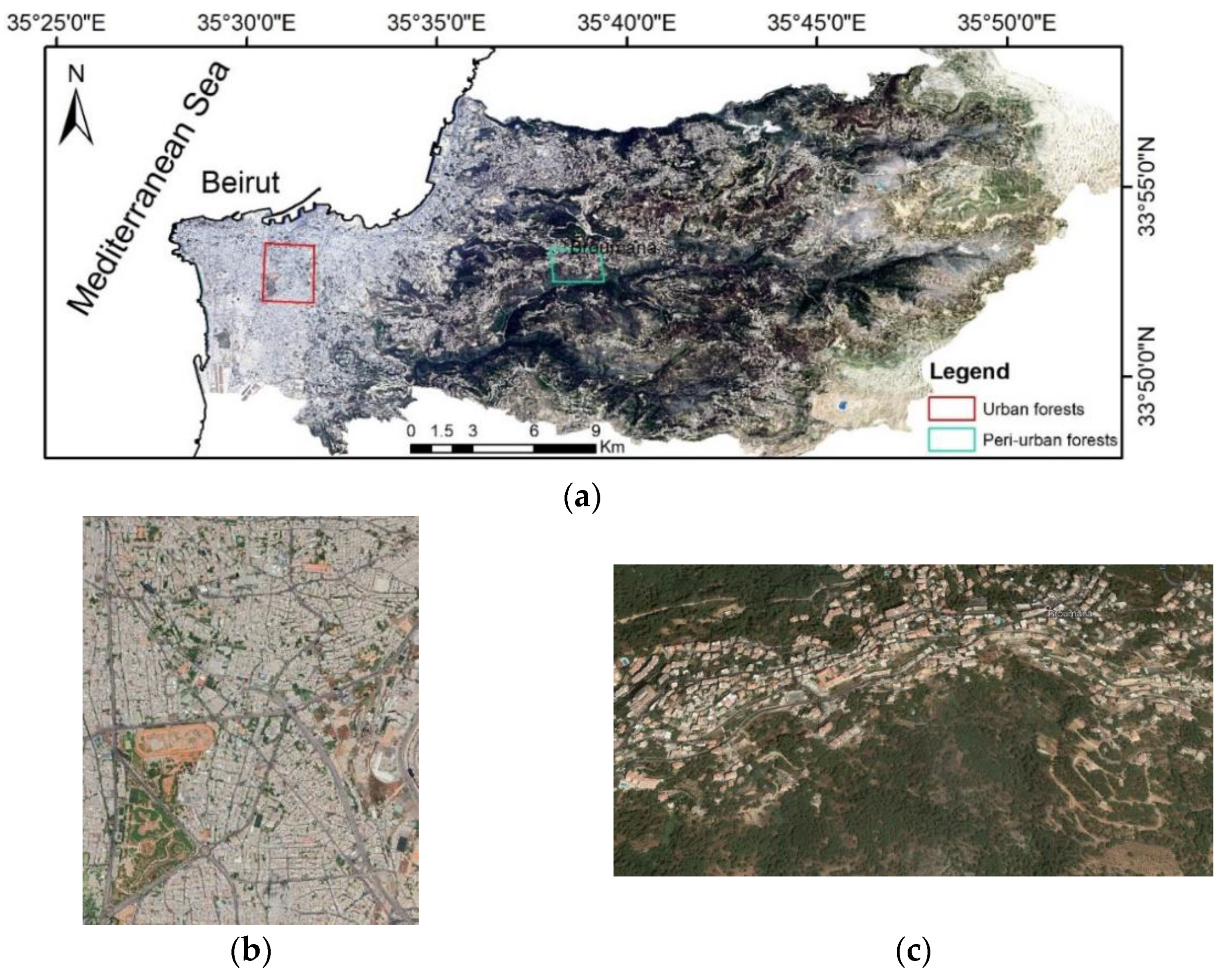
Two different areas were selected in Lebanon, a country that is located in the east of the Mediterranean basin (Figure 1). The size of the first area (urban) is 5.67 Km2, and the size of the peri-urban area is 3.28 Km2.
The study areas have different geographic characteristics. The urban area is located in Beirut, the capital of Lebanon, at sea level, and it is densely populated. The peri-urban area in Broumana is at a higher elevation of about 600 m, and it is characterized by steep to very steep slopes. Nature in the last area suffers from overexploitation by tourism activities. Moreover, the Broumana study area is suffering from the expansion of urban infrastructure and buildings and decrease in forest cover, which adds more stress to the existing cover.
The main soil types for these areas are Eutric Arenosols (AReu), Eutric Cambisols (CMeu), Lithic Leptosols (LPli), and Arenic Luvisols (LVar) [24]. The following features characterize these types of soil: It is (1) either developed on limestone or sandstone lithology, (2) shallow to deep soil, and (3) well drained.
The Mediterranean climate in the study areas can be described in winter as moderate in Beirut and cold in Broumana. In summer, the average temperature in Beirut and Broumana is about 17 °C, and the average yearly precipitation is about 400 mm [25].
2.2. Data
In this research, we deployed European Space Agency (ESA) Sentinel-2 (A and B) products. Sentinel-2A is an optical remote sensing satellite with a spatial resolution that varies between 10 m and 60 m depending on the wavelengths. It also has a temporal resolution of 10 days that can improve to 5 days by being combined with the Sentinel-2B optical satellite. Sentinel-2A and 2B cover wavelengths from 443 nm to 2190 nm and have a spectral resolution that varies between 35 nm (red edge bands) and 580 nm short wavebands.
The selected Sentinel-2 images are level-2 images, meaning that the images are atmospherically corrected, and the pixel values represent surface reflectance. Moreover, the selected images have cloud cover less than or equal to 5%. The dates of acquisition for some selected Sentinel-2 images are listed in Table 1.
These images were retrieved using Google Earth Engine (GEE). Different scripts were written in Java language to retrieve these images (see code below as an example).
var collection = ee.ImageCollection(‘COPERNICUS/S2_SR’) // Source of data
.filterDate(‘2019-01-01’, ‘2019-12-31’) //Date of acquisition
.filterBounds(AreaofStudyBoundaries) // Area of studies
// Pre-filter to get less cloudy granules less than 5 %.
.filter(ee.Filter.lt(‘CLOUDY_PIXEL_PERCENTAGE’,5)) });
2.3. Methods
After selecting the needed remote sensing data for the classification of forests in the urban and peri-urban environments, the next step was to create an efficient and robust classification method.
The suggested new method is a cooperative one that combines two different artificial neural network machine learning algorithms, one being an unsupervised and the other a supervised algorithm.
The first algorithm is UNet [18], a supervised deep learning algorithm, and the second algorithm is self-organizing maps (SOMs) [22,23].
The role of SOMs is to create the training and validation data that help UNet to classify the input image correctly and efficiently. To explain in detail the new cooperative method, the following subsection describes UNet’s structure and functionality.
2.3.1. UNet Network
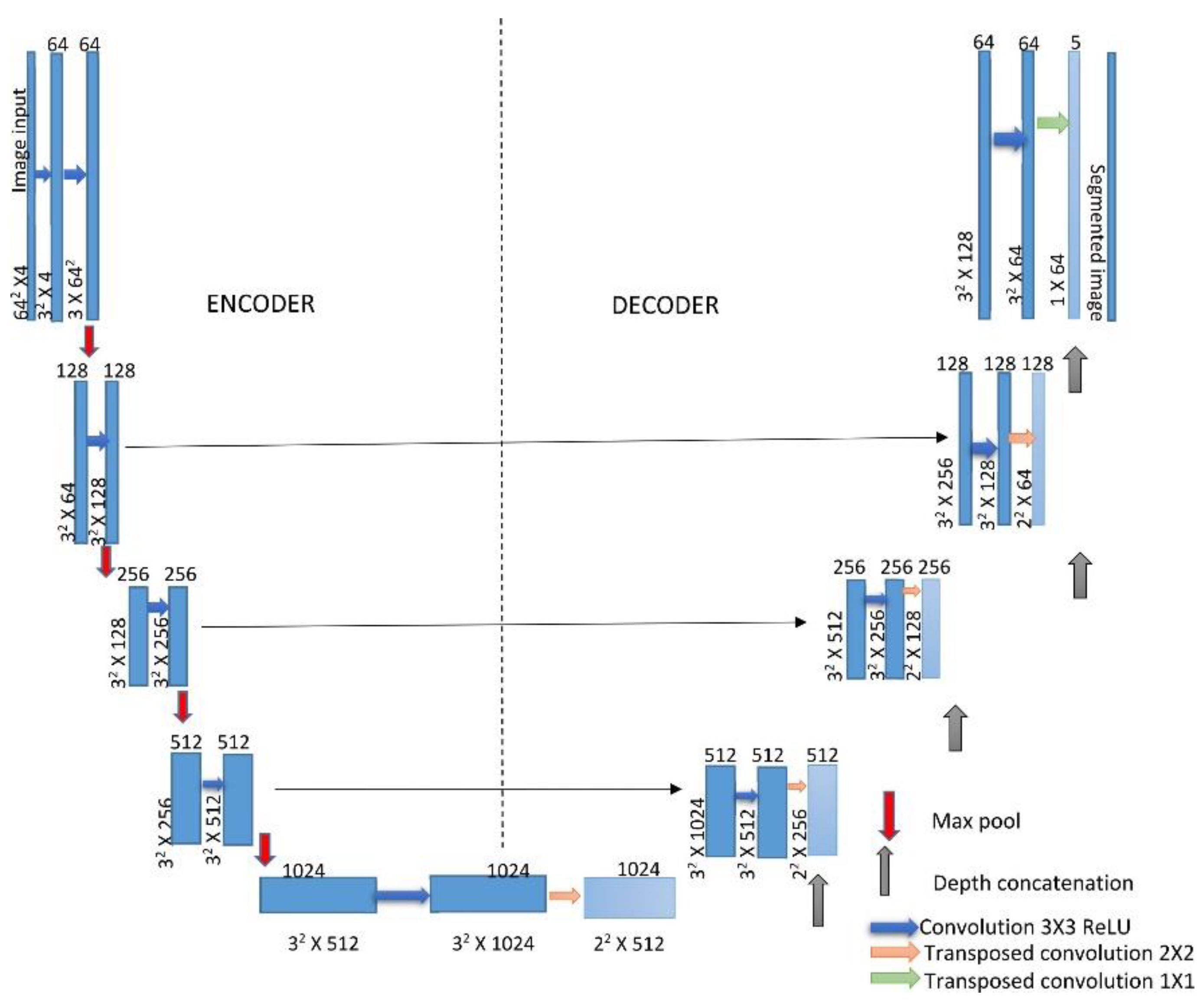
The deep learning architecture UNet [18] was created for use in biomedical image classification. It consists of an encoder network followed by a decoder network. In addition to the requirement of discrimination at pixel level, UNet semantic classification also requires a mechanism to project the discriminative features learned at different stages of the encoder onto the pixel space.
The encoder is the first half of the architecture (Figure 2). Normally, it is a pre-trained classification network such as ResNet [20], where you apply convolution blocks, followed by a maximum pool layer as a downscaling process to encode the input image into feature representations at multiple, different levels.
The decoder is the second half of the architecture (Figure 2). The goal is to semantically project the discriminative features (lower resolution) learned by the encoder onto the pixel space (higher resolution) to obtain a compact and dense classification. The decoder consists of upscaling concatenation followed by regular convolution operations. UNet takes its name from the architecture which, when visualized, appears similar to the letter U, as shown in Figure 2.
As one can notice from the schema, the final number of classes is 5, and one of these classes should be forests.
UNet transforms multi-dimensional input images into classified images. The network does not have a fully connected layer. Only the convolution layers are used. The UNet architecture is based on several layers; these layers can be input 2D or 3D image layers or convolutional layers (2D or 3D) to downsample or upsample (transpose).
Each standard convolution process is activated by a ReLU activation function. A ReLU layer performs a threshold operation to each element of the input, where any value less than zero is set to zero. Max pooling performs downsampling by dividing the input into rectangular pooling regions and computing the maximum of each region.
In the upsampling process, a transposed 2D convolution layer is used, followed by a depth concatenation layer that takes inputs that have the same height and width and concatenates them along the third dimension (channel dimension).
Finally, a Softmax layer (normalized exponential function) [9] is often used as the last activation function of UNet. Its job is to normalize the output of a network to a probability distribution over predicted output classes. The standard Softmax function Sm: is defined by the following Equation (1):
which applies the standard exponential function to each element zi of the input vector z and normalizes these values by dividing by the sum of all these exponentials. In brief, the According to [18] the UNet architecture consists of an encoder and decoder subnetworks each is made of multiple stages, and they are connected by a bridge section. These subnetworks consist of multiple stages. An encoder depth, which specifies the depth of the encoder and decoder subnetworks, sets the number of stages and determines the number of max pools. The stages within the UNet encoder subnetwork consist of two sets of convolutional and ReLU layers, followed by a 2-by-2 max-pooling layer. The decoder subnetwork comprises a transposed convolution layer for upsampling, followed by two sets of convolutional and ReLU layers. The bridge section consists of two sets of convolution and ReLU layers. The bias term of all convolutional layers is initialized to zero. The Convolution layer weights in the encoder and decoder subnetworks are initialized using the ‘He’ weight initialization method [20].
Loss functions are a key part of any machine learning model: they define an objective against which the performance of the UNet model is measured, and the setting of weight parameters learned by the model is determined by minimizing a chosen loss function. UNet uses the cross-entropy loss (log loss) function [26], which is just a straightforward modification of the likelihood function with logarithms.
The cross-entropy predicts class probability and then compares it to the actual class desired output. A loss is calculated that penalizes the probability based on how far it is from the actual expected value. The penalty is logarithmic yielding a large score for large differences close to 1 and small score for small differences tending to 0.
Cross-entropy is used when adjusting model weights during training. The aim is to minimize the loss, i.e., the smaller the loss, the better the model. A perfect model has a cross-entropy loss of 0. Cross-entropy is defined as Equation (2):
where ti is the truth label and pi is the Softmax probability for the ith class.
Normally, UNet requires a large training dataset to function properly [27]; this is also proven in the experiments. Therefore, extracting enough training datasets may not be feasible, especially if the image is of medium spatial resolution and the features are hard to discern.
2.3.2. Self-Organizing Maps (SOMs)
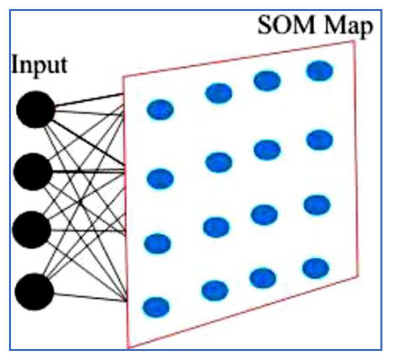
Self-organizing maps (SOMs) [22,23] are an unsupervised neural network method. SOMs convert patterns of arbitrary dimensionality into responses of two-dimensional arrays of neurons. One of the most important characteristics of SOMs is that the feature map preserves the neighborhood relations of the input pattern.
A typical SOM structure is given in Figure 3. It consists of two layers: an input layer and an output layer. The number of input neurons is equal to the dimensions of the input data. The output neurons are arranged in a two-dimensional array.
The network is composed of an orthogonal grid of cluster units (neurons), each of which is associated with N internal weights for the N layers of the satellite image. At each step in the training phase, the cluster unit with weights that best match the input pattern is elected as the winner, usually using the minimum Euclidean distance as in Equation (3):
where x is the input vector, is the weight of the wining unit l at iteration k, and is the weight for neuron I at iteration k. The winning unit and a neighborhood around it are then updated in such a way that their internal weights are closer to the presented input. All the neurons within a certain neighborhood around the leader participate in the weight-update process. This learning process can be described by the iterative procedure as in Equation (4):
where is a smoothing kernel defined over the winning neuron. This kernel is written in terms of the Gaussian function as in Equation (5):
, where T0 is the total number of iterations. is the initial learning rate, and it is equal to 0.1. The learning rate is updated in every iteration. is the search distance at iteration k, which can initially be half the length of the network. After SOMs converge to a balanced state, the original image is mapped from a high-dimension to a low-dimension space. The number of clusters in this space is equal to the number of neurons in the SOMs network.
2.3.3. SO-UNet
Although UNet’s performance improves with the provision of large training samples, obtaining enough training samples is not feasible for medium- or low-spatial resolution satellite remote sensing images. Transfer learning can effectively alleviate this problem by transferring the knowledge from the results obtained by the unsupervised SOMs to the target—in our case, the supervised deep learning network. Furthermore, the transfer of knowledge from self-learning algorithms to SOMs can improve the accuracy of UNet [28].
There are four main transfer learning categories: instance-based, mapping-based transfer, network-based deep, and adversarial-based [29]. These transfer schemes work on partial information such as partial training and parameters using different structures. However, our main objective is to transfer the complete training set to the target deep learning algorithm UNet. SOMs is capable of providing complete training datasets to UNet with no guidance (unsupervised). We call this scheme self-organizing transfer learning (Figure 4).
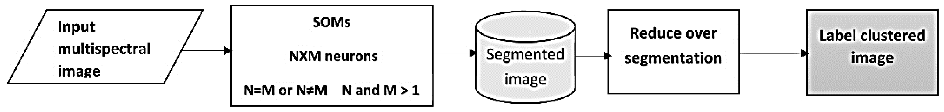
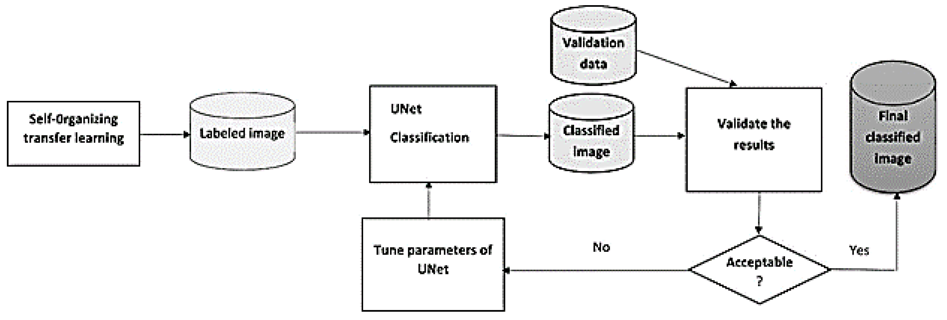
SO-UNet consists of SOMs as a source for transferring training datasets to UNet. SOMs are modified according to [23] to remove over-classification. Then, the results obtained by SOMs are labeled according to the collected training datasets, and then they are fed to UNet. Furthermore, SO-UNet implements different phases to produce a final classified image (Figure 5): (1) Retrieve corrected multi-spectral image; (2) clip the image to specific areas; (3) select high spatial resolution wavelengths (VNIR); (4) apply SO transfer learning; (5) run UNet with different settings; (6) validate the results; (7) tune UNet and repeat from 5 if not acceptable. UNet’s parameters to be tuned include the number of iterations, size of the image, and size of the convolution matrix.
2.4. Verification Methods
The accuracy of the results is computed based on the confusion matrix method [30]. The matrix is of size m × m associated with a classifier that shows the predicted and observed classification (Table 2).
Using Table 2, the computation of the overall accuracy (OA) for each experiment is based on Equation (6):
T1 and T2 can be actual or predicted samples, and these samples are either positive when the actual sample matches the predicted or negative otherwise.
Kappa coefficient κ [31] is another metric method for accuracy assessment. The Kappa coefficient is frequently used to test interrater agreement (Equation (7)). The coefficient value ranges from the worst agreement for value -1 to the perfect one for value +1.
where is the observed proportionate agreement (overall accuracy Equation (6)), and is the overall random agreement probability (Equation (8)). According to [32], Kappa value = 0 indicates no agreement, while > 0–0.20 slight, 0.20–0.40 fair, 0.40–0.60 moderate, 0.60–0.80 substantial, and 0.80–1 almost perfect agreement.
3. Experimental Results
3.1. Data Preparation
For each study area, four images with different dates were selected. One date is in the dry hot season (summer), another in the spring season. The remaining two images are in the fall season and the wet cold winter season. The size of the images is 222 × 165 pixels for peri-urban, and 207 × 287 for urban. There are eight images, among which every four images represent a different study area and different seasons in the year 2019.
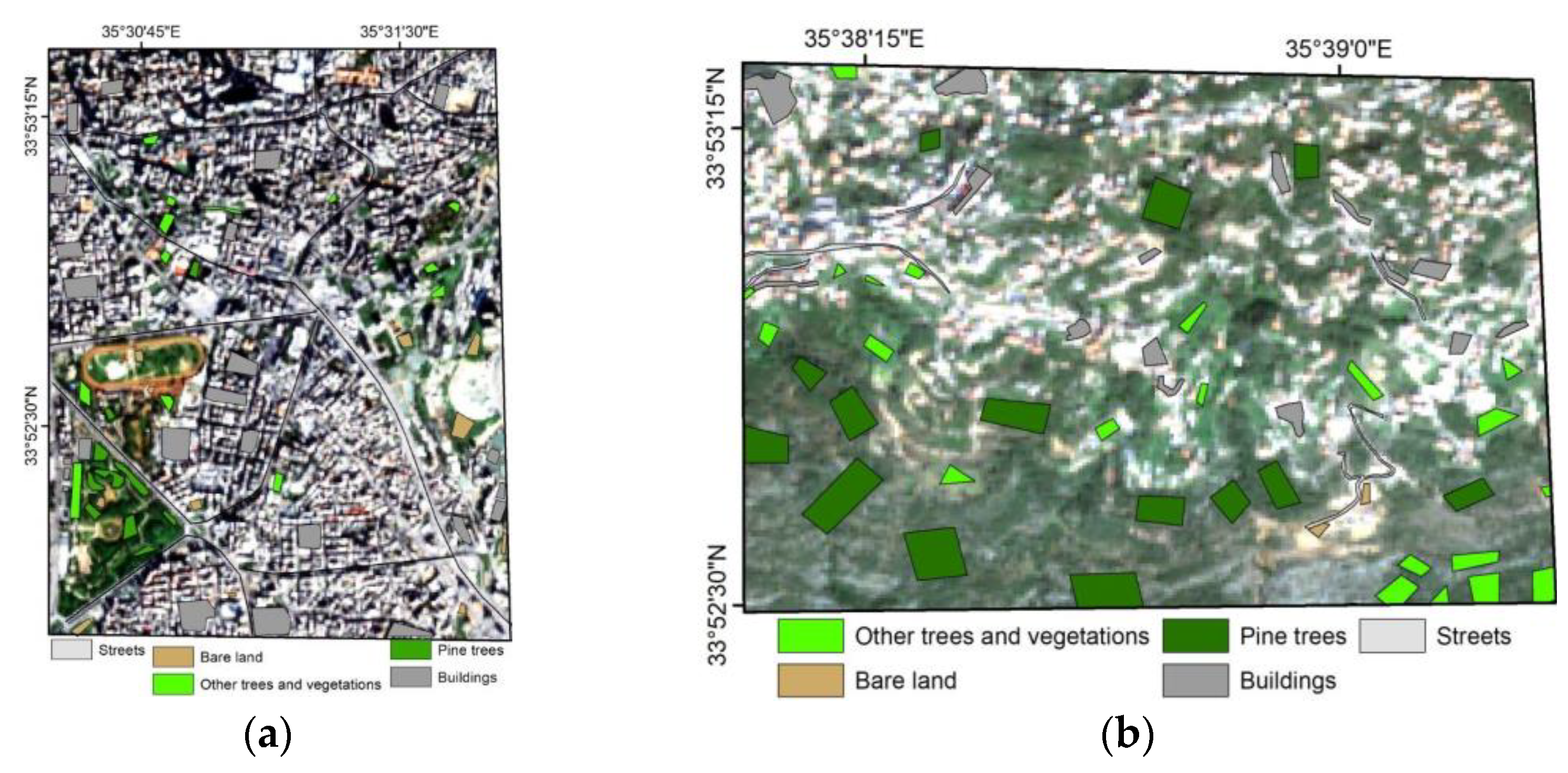
Two reasons justify our selection of the study areas and the temporal images: (1) to check the effect of change in the environment on the efficiency and accuracy of the new method; and (2) to verify the robustness of the new method concerning changes in image quality due to seasonal variations. The following images (Figure 6a,b) show some of the training sets for each study area over a Sentinel-2 image.
3.2. Different Algorithm Setup
Self-organizing maps (SOMs) are initiated with a specific number of neurons and iterations. The rule for network size is based on the rule (N + [1…L]), where N is the number of classes and L ≥ 1 is the balance scale between under and over-segmentation. The L value is an odd number if N is odd, and even otherwise. In this research, N = 5, and L is equal to 1 or 3. The number of iterations is selected to be 1000, but SOMs can halt before completing all the iterations after reaching a balanced state (SOMs’ weights do not change by more than a defined threshold).
In our case, UNet initially consists of 58 layers (encoder depth = 4). This means that four Max pools are used. Each image in UNet is used to extract 160 randomly positioned patches with a size of 64 × 64 pixels. The number of classes is 5 (buildings, pine trees, streets, bare land, and other trees), and the input image size is patchsize × numberofbands. numberofbands represents four different wavelengths selected from Sentinel-2 images. The number of epochs is initially set to 100, and the number of mini-batches is 16. A mini-batch is a subset of the training set that is used to evaluate the gradient of the loss function and update the weights. Mini-batch training is a combination of batch and stochastic training.
This means that the total number of iterations is 1000 (Equation (9)). Being the major forest cover in the study areas, pine is classified out of the different forest types.
Niter is the number of iterations, Nep is the number of epochs, Npat is the number of patches, and Mpat is the number of mini-batches.
3.3. Results and Discussion
In the experiments, UNet is run first alone and trained using the collected samples. Then, SO-UNet is run next with training samples supplied by SOMs’ labeled results. Changing SOM and UNet parameters is another way to check the efficiency and robustness of the created method compared to UNet.
The following graphs show the accuracies and mini-batch loss for four different runs of UNet and SO-UNet. Each of the listed methods was run twice—one time for the urban image and another for the peri-urban. The two methods were run for different setups (Table 3), where only the image size, mini-batch size, and patches per image were the variables such that the total number of iterations is always 1000 according to Equation (8). This also means that the number of epochs remained fixed. The classified images for urban and peri-urban areas are for Sentinel-2 acquired on 5 February 2019.
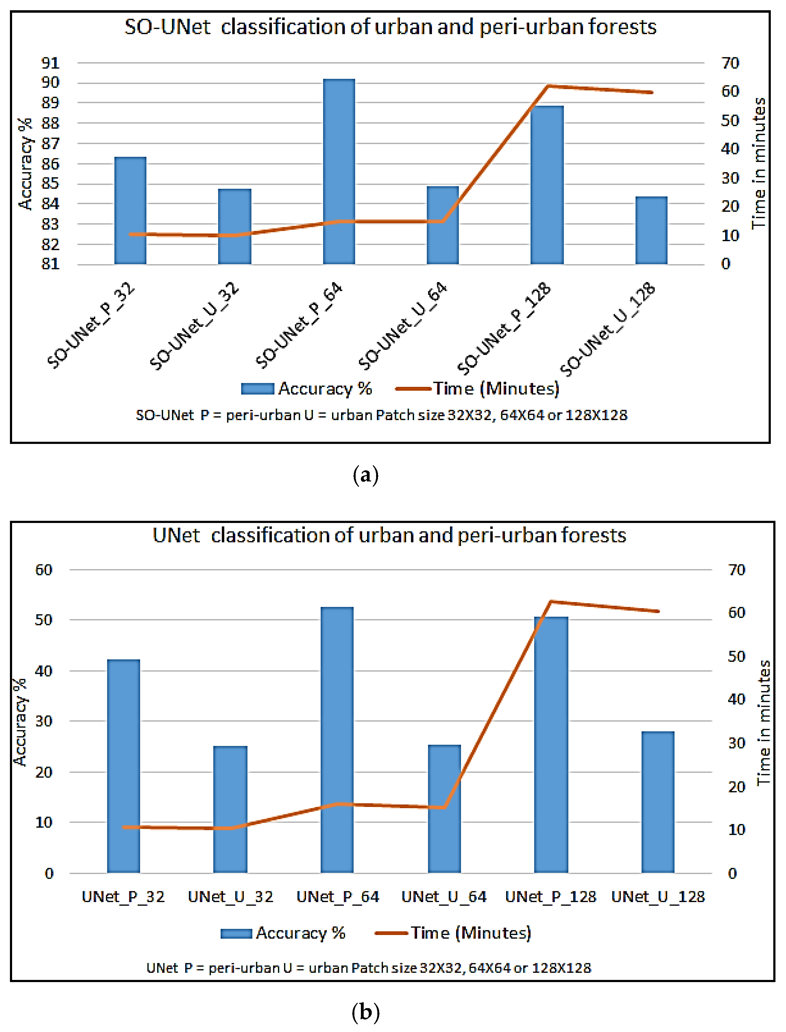
The graphs in Figure 7a,b show the accuracy and speed for UNet and SO-UNet in the classification of urban and peri-urban forests.
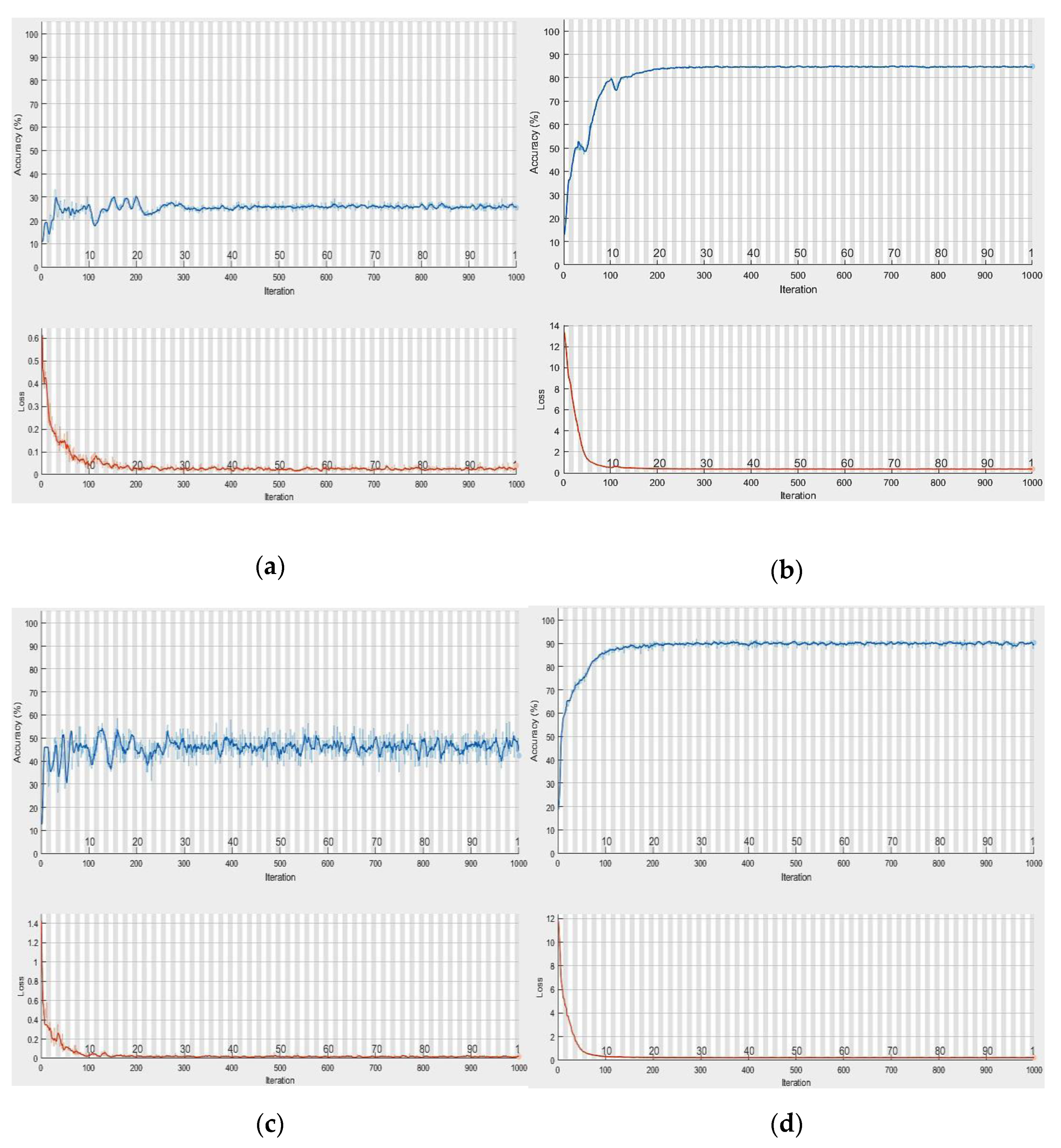
The results show that as we increase patch size (image size), the time required to cover 1000 iterations is longer. Moreover, increasing patch size increases the demands for computer resources, such as memory central unit processor (CPU) use. The accuracy of UNet increases slightly with the increase in patch size, but that is not the case with SO-UNet, where the patch size 64 × 64 remains the best setting. SO-UNet remains the best in speed compared to UNet. Moreover, analyzing the graphs in Figure 8a–d, one can conclude that SO-UNet is more stable than UNet (fluctuating accuracy during the run). Finally, analyzing the loss function, one can clearly see that the values provided by UNet are lower than those by SO-UNet due to training UNet with insufficient training samples compared to training SO-UNet with complete samples provided by SOMs.
Based on the previous experiments, SO-UNet adapted the settings that provided the highest accuracy (patch size = 64 × 64 and mini-batch size = 16). These settings were used to classify other Sentinel-2 images, and the results of SO-UNet were compared to those of UNet. Table 4 shows the accuracies of the classification results for both SO-UNet and UNet.
It can be seen in Table 4 that classified urban and peri-urban images by SO-UNet maintained a stable range of accuracies between 80.5% and 85.6%, whereas the classification results by UNet had fluctuating accuracies that ranged between 18.2% and 45.2%.
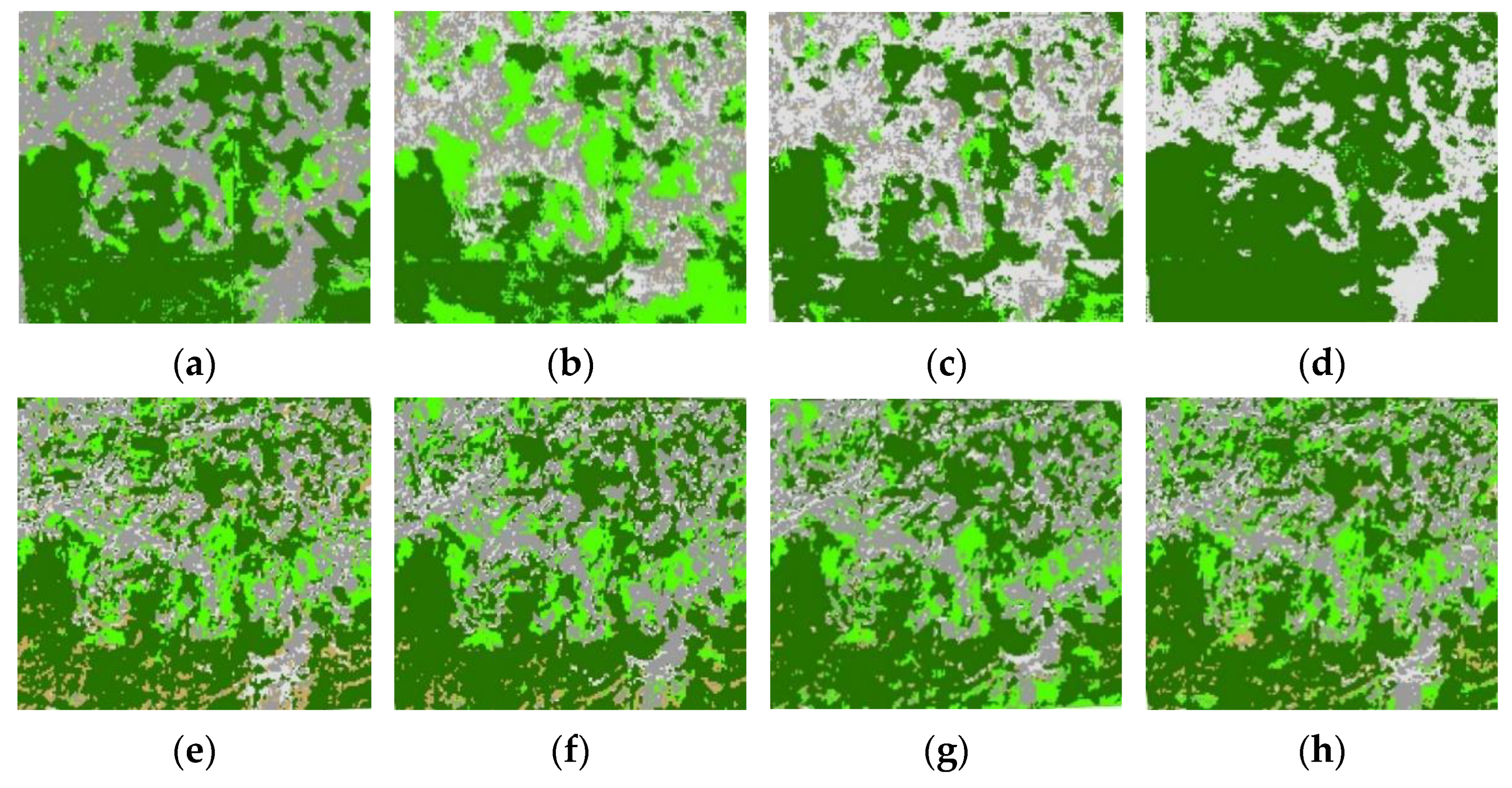
The classification results of peri-urban temporal images by UNet and SO-UNet are shown in Figure 9a–h. The first row of the images represents the peri-urban classified images by UNet, whereas the second row represents classified peri-urban images by SO-UNet. The UNet classification of the forests is different in each image, whereas the results of SO-UNet are almost comparable. These results prove the instability of UNet in the classification of complex images, such as remote sensing images.
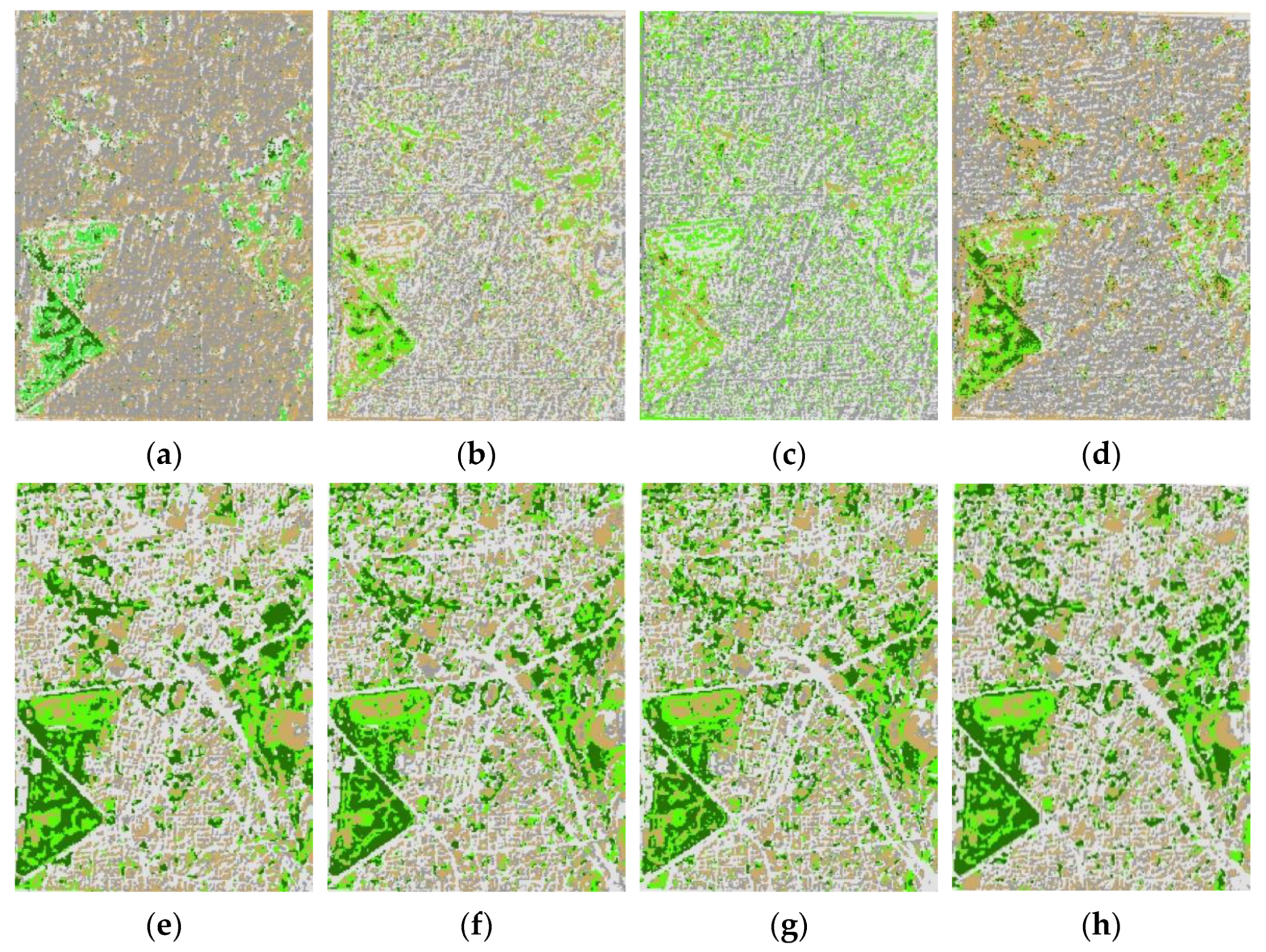
UNet and SO-UNet classification of urban forests using different temporal images is displayed in Figure 10a–h. Inspecting the classified images by SO-UNet visually, one can easily see the resemblance of many features between these images that were collected in different seasons, which is not the case in UNet’s images. This again proves the efficiency and stability of SO-UNet compared to UNet. Urban forests are one of the most complex features to discern from remote sensing images using any known advanced classification techniques. However, cooperative techniques can help to improve feature discrimination tasks.
4. Conclusions
In this research, a new deep learning classification method was created (SO-UNet). It is based on two different machine learning algorithms, i.e., SOMs and UNet. SO-UNet can classify moderate spatial resolution images in a semi-supervised way, unlike supervised deep learning UNet. The efficiency of the new method, SO-UNet, in the classification of urban and peri-urban forests is evident. SO-UNet provided noticeably higher accuracy compared to UNet. In addition, the classification of multi-temporal images proved the stability of the new method in extracting the forests from complex environments. The novelty of this research is the creation of a semi-supervised deep learning method that can pave the way toward improving deep learning in general. It is considered a first attempt in creating a semi-supervised deep learning. Finally, the work can be extended to include lower-resolution remote sensing images.
Author Contributions
Conceptualization, M.M.A.; methodology: M.M.A.; software M.M.A.; validation M.M.A.; formal analysis M.M.A.; investigation M.M.A.; resources M.M.A.; data curation M.M.A.; writing—original draft preparation M.M.A.; writing—review and editing, M.M.A. and M.L.; visualization M.M.A.; supervision M.M.A. and M.L.; project administration, M.M.A. and M.L; funding acquisition M.M.A. and M.L. Both authors have read and agreed to the published version of the manuscript.
Funding
This research was funded by CNRS-L and CNRS.
Data Availability Statement
Data resulted from this research can be requested from the corresponding author.
Acknowledgments
The author would like to thank CNRS-L for the support provided to the project in cooperation with the Italian Institute of Biology Research on Terrestrial Ecosystems (IBAFIRET) of the National Research Council (CNR), within the Joint Bilateral Agreement CNRS-L/CNR “Monitoring urban and peri-urban green infrastructure as early detection of stress and environmental quality”, biennial program 2018–2019.
Conflicts of Interest
The authors declare no conflict of interest.
References
- Dobbs, C.; Eleuterio, A.A.; Amaya, J.D.; Montoya, J.; Kendal, D. The benefits of urban and peri-urban forestry. Unasylva J. 2018, 69, 22–29. [Google Scholar]
- Dobbs, C.; Escobedo, F.; Zipperer, W. A framework for developing urban forest ecosystem services and goods indicators. Landsc. Urban Plan. J. 2011, 99, 196–206. [Google Scholar] [CrossRef]
- Lausc, A.; Erasmi, S.; King, D.; Magdon, P.; Heurich, M. Understanding forest health by remote sensing Part I—A review of spectral traits, processes and remote sensing characteristics. Remote Sens. 2016, 9, 129. [Google Scholar] [CrossRef] [Green Version]
- Garnier, E.; Lavorel, S.; Ansquer, P.; Castro, H.; Cruz, P.; Dolezal, J.; Eriksson, O.; Fortunel, C.; Freitas, H.; Golodets, C.; et al. Assessing the effects of land-use change on plant traits, communities and ecosystem functioning in grasslands: A standardized methodology and lessons from an application to 11 European sites. Ann. Bot. 2007, 99, 967–985. [Google Scholar] [CrossRef] [PubMed] [Green Version]
- Lin, Y.; Jiang, M.; Yao, Y.; Zhang, L.; Lin, J. Use of UAV oblique imaging for the detection of individual trees in residential environments. Urban For. Urban Green. 2015, 14, 404–412. [Google Scholar] [CrossRef]
- Näsi, R.; Honkavaara, E.; Blomqvist, M.; Lyytikäinen-Saarenmaa, P.; Hakala, T.; Viljanen, N.; Kantola, T.; Holopainen, M. Remote sensing of bark beetle damage in urban forests at individual tree level using a novel hyperspectral camera from UAV and aircraft. Urban For. Urban Green. 2018, 30, 72–83. [Google Scholar] [CrossRef]
- Awad, M. Forest mapping: A comparison between hyperspectral and multispectral images and technologies. Springer J. For. Res. 2018, 29, 1395–1405. [Google Scholar] [CrossRef]
- ESA. Copernicus Open Access Hub. Available online: https://scihub.copernicus.eu/dhus/#/home (accessed on 20 July 2019).
- Goodfellow, I.; Bengio, Y.; Courville, A. Deep Learning; The MIT Press: New York, NY, USA, 2016; 599p. [Google Scholar]
- Liu, M.; Han, Z.; Chen, Y.; Liu, Z.; Han, Y. Tree Species Classification of LiDAR Data based on 3D Deep Learning. Measurement 2021, 177. [Google Scholar] [CrossRef]
- Sylvain, J.; Drolet, G.; Brown, N. Mapping dead forest cover using a deep convolutional neural network and digital aerial photography. ISPRS J. Photogramm. Remote Sens. 2019, 156, 14–26. [Google Scholar] [CrossRef]
- Venkatesan, R.; Baoxin, L. Convolutional Neural Networks in Visual Computing: A Concise Guide, 1st ed.; CRC Press: Boca Raton, FL, USA, 2017; 186p, ISBN 978-1-351-65032-8. [Google Scholar]
- Sjöqvist, H.; Längkvist, M.; Javed, F. An Analysis of Fast Learning Methods for Classifying Forest Cover Types. Appl. Artif. Intell. 2020, 34, 691–709. [Google Scholar] [CrossRef]
- Breiman, L. Random forests. Machine Learn. 2001, 45, 5–32. [Google Scholar] [CrossRef] [Green Version]
- Pal, M.; Mather, P. Support vector machines for classification in remote sensing. Int. J. Remote Sens. 2005, 26, 1007–1011. [Google Scholar] [CrossRef]
- MacMichael, D.; Si, D. Machine Learning Classification of Tree Cover Type and Application to Forest Management. Int. J. Multimed. Data Eng. Manag. (IJMDEM) 2018, 9, 21. [Google Scholar] [CrossRef] [Green Version]
- Wagner, F.; Sanchez, A.; Tarabalka, Y.; Lotte, R.; Ferreira, M.; Aidar, M.; Gloor, E.; Phillips, O.; Aragão, L. Using the U-net convolutional network to map forest types and disturbance in the Atlantic rainforest with very high-resolution images. Remote Sens. Ecol. Conserv. 2019. [Google Scholar] [CrossRef] [Green Version]
- Ronneberger, O.; Fischer, P.; Brox, T. U-Net: Convolutional Networks for Biomedical Image Segmentation. Springer Med Image Comput. Comput. Assist. Interv. 2015, 9351, 234–241. [Google Scholar] [CrossRef] [Green Version]
- Cao, K.; Zhang, X. An Improved Res-UNet Model for Tree Species Classification Using Airborne High-Resolution Images. Remote Sens. 2020, 12, 1128. [Google Scholar] [CrossRef] [Green Version]
- He, K.; Zhang, X.; Ren, S. Deep Residual Learning for Image Recognition. In Proceedings of the 2016 IEEE Conference on Computer Vision and Pattern Recognition (CVPR), Las Vegas, NV, USA, 27–30 June 2016; pp. 770–778. [Google Scholar]
- Soni, A.; Koner, R.; Villuri, V.G.K. M-UNet: Modified U-Net Segmentation Framework with Satellite Imagery. In Proceedings of the Global AI Congress 2019; Mandal, J., Mukhopadhyay, S., Eds.; Advances in Intelligent Systems and Computing; Springer: Singapore, 2020; Volume 1112. [Google Scholar] [CrossRef]
- Awad, M.; Chehdi, K.; Nasri, A. Multi-component Image Segmentation Using Genetic Algorithms and Artificial Neural Network. IEEE Geosci. Remote Sens. Lett. 2007, 4, 571–575. [Google Scholar] [CrossRef]
- Awad, M. An unsupervised Artificial Neural Network method for satellite image segmentation. Int. Arab. J. Inf. Technol. (IAJIT) 2010, 7, 199–205. [Google Scholar]
- Darwish, T.; Khawlie, M.; Jomaa, I.; Abou Daher, M.; Awad, M.; Masri, T.; Shaaban, A.; Faour, G.; Bou Khair, R.; Abdallah, C.; et al. Soil Map of Lebanon 1:50000; National Council for Scientific Research: Beirut, Lebanon, 2006; 367p. [Google Scholar]
- NASA. Power Data Access Viewer. Available online: https://power.larc.nasa.gov/data-access-viewer/ (accessed on 11 August 2019).
- Kevin, M. Machine Learning: A Probabilistic Perspective; MIT: Cambridge, MA, USA, 2012; 1027p, ISBN 978-0262018029. [Google Scholar]
- Huang, J.; Nowack, R. Machine Learning Using U-Net Convolutional Neural Networks for the Imaging of Sparse Seismic Data. Pure Appl. Geophys. 2020, 177, 2685–2700. [Google Scholar] [CrossRef]
- Yang, J.; Zhao, Y.; Chan, J. Learning and transferring deep joint spectral–spatial features for hyperspectral classification. IEEE Trans. Geosci. Remote Sens. 2017, 55, 4729–4742. [Google Scholar] [CrossRef]
- Tan, C.; Sun, F.; Kong, T.; Zhang, W.; Yang, C.; Liu, C. A Survey on Deep Transfer Learning. In Artificial Neural Networks and Machine Learning-Lecture Notes in Computer Science 11141; Kůrková, V., Manolopoulos, Y., Hammer, B., Iliadis, L., Maglogiannis, I., Eds.; Springer: Cham, Switzerland, 2018. [Google Scholar] [CrossRef] [Green Version]
- Congalton, R. A review of assessing the accuracy of classifications of remotely sensed data. Remote Sens. Environ. 1991, 37, 35–46. [Google Scholar] [CrossRef]
- Cohen, J. A coefficient of agreement for nominal scales. Educ. Psychol. Meas. 1960, 20, 37–46. [Google Scholar] [CrossRef]
- Koch, G. The measurement of observer agreement for categorical data. Biometrics 1977, 33, 159–174. [Google Scholar]
Figure 1.
Study areas. (a) Location; (b) urban forests—Beirut; and (c) peri-urban forests—Broumana (Google Earth).
Figure 1.
Study areas. (a) Location; (b) urban forests—Beirut; and (c) peri-urban forests—Broumana (Google Earth).

Figure 2.
Suggested UNet scheme for this research work.

Figure 3.
SOMs [23].
Figure 3.
SOMs [23].

Figure 4.
Self-organizing transfer learning.

Figure 5.
Self-organizing deep learning (SO-UNet).

Figure 6.
Training samples on the Sentinel-2 image of an (a) urban area and (b) peri-urban area.

Figure 7.
Accuracy and efficiency of urban and peri-urban classification by (a) SO-UNet and (b) UNet.
Figure 7.
Accuracy and efficiency of urban and peri-urban classification by (a) SO-UNet and (b) UNet.

Figure 8.
Patch size 64 × 64; (a) UNet urban; (b) SO-UNet urban; (c) UNet peri-urban; and (d) SO-UNet peri-urban.
Figure 8.
Patch size 64 × 64; (a) UNet urban; (b) SO-UNet urban; (c) UNet peri-urban; and (d) SO-UNet peri-urban.

Figure 9.
Classification of peri-urban forests: (a–d) UNet and (e–h) SO-UNet.

Figure 10.
Classification of urban forests: (a–d) UNet and (e–h) SO-UNet.


Table 1.
A list of selected Sentinel-2 images.
| Date of Acquisition |
|---|
| 5 February 2019 |
| 21 May 2019 |
| 30 July 2019 |
| 17 November 2019 |
Table 2.
Confusion matrix format.
| Predicted | |||
|---|---|---|---|
| T1 | T2 | ||
| Actual | T1 | True | False |
| T2 | False | True | |
Table 3.
UNet and SO-UNet classification of Sentinel-2 images with different settings.
| Method | Area | Number of Iterations | Accuracy % | Mini-Batch Loss | Time (Minutes) | Patch Size | Mini-Batch Size |
|---|---|---|---|---|---|---|---|
| UNet | Urban | 1000 | 25.39 | 0.0398 | 15.2 | 64 × 64 | 16 |
| SO-UNet | Urban | 1000 | 84.87 | 0.3813 | 14.8 | 64 × 64 | 16 |
| UNet | Peri-Urban | 1000 | 52.69 | 0.0094 | 16.1 | 64 × 64 | 16 |
| SO-UNet | Peri-Urban | 1000 | 90.22 | 0.2275 | 15 | 64 × 64 | 16 |
| UNet | Urban | 1000 | 25.08 | 0.0657 | 10.46 | 32 × 32 | 32 |
| SO-UNet | Urban | 1000 | 84.74 | 0.3846 | 10.28 | 32 × 32 | 32 |
| UNet | Peri-Urban | 1000 | 42.36 | 0.0174 | 10.73 | 32 × 32 | 32 |
| SO-UNet | Peri-Urban | 1000 | 86.32 | 0.2628 | 10.67 | 32 × 32 | 32 |
| UNet | Urban | 1000 | 28.14 | 0.0187 | 60.3 | 128 × 128 | 12 |
| SO-UNet | Urban | 1000 | 84.34 | 0.3881 | 59.82 | 128 × 128 | 12 |
| UNet | Peri-Urban | 1000 | 50.7 | 0.0105 | 62.62 | 128 × 128 | 12 |
| SO-UNet | Peri-Urban | 1000 | 88.87 | 0.2381 | 61.8 | 128 × 128 | 12 |
Table 4.
Results of Sentinel-2 classification by UNet and SO-UNet.
| Method | Area | Date | Accuracy% |
|---|---|---|---|
| UNet | Peri-Urban | 21 May 2019 | 38.4 |
| SO-UNet | Peri-Urban | 21 May 2019 | 85.6 |
| UNet | Urban | 21 May 2019 | 19.7 |
| SO-UNet | Urban | 21 May 2019 | 80.5 |
| UNet | Peri-Urban | 17 November 2019 | 45.2 |
| SO-UNet | Peri-Urban | 17 November 2019 | 82.5 |
| UNet | Urban | 17 November 2019 | 20.8 |
| SO-UNet | Urban | 17 November 2019 | 84.7 |
| UNet | Peri-Urban | 30 July 2019 | 37.8 |
| SO-UNet | Peri-Urban | 30 July 2019 | 80.5 |
| UNet | Urban | 30 July 2019 | 18.2 |
| SO-UNet | Urban | 30 July 2019 | 83.25 |
Publisher’s Note: MDPI stays neutral with regard to jurisdictional claims in published maps and institutional affiliations. |
© 2021 by the authors. Licensee MDPI, Basel, Switzerland. This article is an open access article distributed under the terms and conditions of the Creative Commons Attribution (CC BY) license (https://creativecommons.org/licenses/by/4.0/).
Share and Cite
MDPI and ACS Style
Awad, M.M.; Lauteri, M. Self-Organizing Deep Learning (SO-UNet)—A Novel Framework to Classify Urban and Peri-Urban Forests. Sustainability 2021, 13, 5548. https://0-doi-org.brum.beds.ac.uk/10.3390/su13105548
AMA Style
Awad MM, Lauteri M. Self-Organizing Deep Learning (SO-UNet)—A Novel Framework to Classify Urban and Peri-Urban Forests. Sustainability. 2021; 13(10):5548. https://0-doi-org.brum.beds.ac.uk/10.3390/su13105548
Chicago/Turabian StyleAwad, Mohamad M., and Marco Lauteri. 2021. "Self-Organizing Deep Learning (SO-UNet)—A Novel Framework to Classify Urban and Peri-Urban Forests" Sustainability 13, no. 10: 5548. https://0-doi-org.brum.beds.ac.uk/10.3390/su13105548
Note that from the first issue of 2016, this journal uses article numbers instead of page numbers. See further details here.