Slime Mold Algorithm for Optimal Reactive Power Dispatch Combining with Renewable Energy Sources

Abstract

The optimal reactive power dispatch (ORPD) is a complex, nonlinear, and constrained optimization problem. This paper presents the application of a new metaheuristic optimization technique called the slime mold algorithm (SMA) for solving the developed objective function of ORPD combining with renewable energy sources. The presented objective function is to minimize the total operating cost of the system through the minimization of all reactive power costs, total real power loss, voltage deviation of load buses, the system overload and improve voltage stability. The formulation of the ORPD problem combining with renewable energy sources with five different objective functions is then converted to a coefficient single objective function achieving various operating constraints. The SMA technique has been tested and proven on the IEEE 30-bus system and IEEE-118 bus system using different scenarios. Five different scenarios, with and without renewable energy sources, are presented on the two-test system and the simulation results of the SMA is compared to some optimization techniques from the literature under the same test system data, optimal control variables, and operational constraints. The superiority and effectiveness of the SMA are proven through comparison with the other obtained results from recently published optimization techniques.

1. Introduction

Presently, the power system network urgently needs to operate at whole capacity because of the imbalanced investment in power system sectors. Therefore, there is consensus among power network operators to develop the existing distribution as well as the transmission systems by installation of new lines and/or adding power grid stations to force the system to be more reliable, efficient and smart. In addition, the alternative solution regards employing the existing system without upgrading, by optimally setting the control parameters of the system which turn in enhance the effectiveness of the system. This process may be achieved during the technical study called optimal power flow (OPF) that is used in power system networks for the minimization of mainly the operating cost and real power transmission losses by obtaining the optimized control variables of the system. Moreover, OPF is consists of two sub-problems, one called economic dispatch and the other optimal reactive power dispatch (ORPD) [1,2].

Optimal reactive power dispatch performs a considerable role in the planning and economic operations of modern power networks. During the use of real power in the system, the reactive power should be circulated in the system [3,4]. The reactive power has a considerable impact on transmitted real power and voltage stability within the power system networks. Therefore, it is necessary to estimate the ORPD. Due to the behavior of the concerned control variables related to voltage control aspects involved in the system components (i.e., reactive compensators, tap-changing transformers, etc.), ORPD is considered an extremely nonlinear complex problem. The ORPD is employed to adjust the control variables’ parameters to accomplish the considered objective function [5,6].

In the last decade, renewable energy sources (RESs) such as wind energy, microturbine generators, solar energy, and biomass are participating in reducing system power losses as well as improving the security and reliability of the power system [7,8]. Moreover, RESs have a major impact on the electricity market where they are required to define the reactive power for the system to meet the considered objective function [9].

In the literature, there are different objective functions employed in ORPD considering equality and inequality constraints. The widely used objective functions are minimizations of both real power losses and transmission cost, enhancement of the voltage profile, and voltage stability maximization [10,11,12].

Conventional mathematical approaches, such as interior-point [13], quadratic programming [14] and linear programming [15] are extensively applied for solving the ORPD problem. In [16], the Lagrangian decomposition approach is presented for solving ORPD to minimize the reactive power exchange cost between areas of multi-area power systems. These conventional methods suffer from drawbacks. They are unable to converge to the closest optimal global solution. Furthermore, they are limited with requirements for non-convexity, differentiability, and continuity of the considered objective function. These classical techniques cannot provide a precise solution to the present form of the ORPD problem. Therefore, numerous optimization techniques are used to provide an accurate solution to the ORPD problem.

At present, metaheuristic optimization techniques overcome the previously stated limitations. The meta-heuristics have essential effectiveness through the fast search of huge solution spaces to avoid local solutions and find global solutions. Presently, various metaheuristic optimization techniques are proposed to solve the ORPD problem. Moth-flame optimization (MFO) is used in [17] to explore the optimal control variables for obtaining the minimum total real power loss and improve the voltage profile. The authors in [18] presented the oppositional krill herd algorithm (OKHA) for solving the ORPD problem based on both a single and multi-objective function based on the minimization of the real power losses and total voltage deviations. The proposed OKHA was implemented on the two IEEE test systems incorporating a unified power flow controller. The gray wolf optimizer (GWO) is employed also in [19] to minimize both the real power loss and total voltage deviation. In [20], the harmony search algorithm (HSA) is introduced for solving the ORPD problem to optimize separately the real transmission loss, voltage profile, and voltage stability based on the optimal settings of the control variables.

On the other hand, hybrid techniques are used for solving ORPD, where different metaheuristic optimization approaches are used together to gather the advantages of different techniques simultaneously. Some of these hybrid techniques are hybrid particle swarm optimization and imperial competitive algorithms (PSO-ICA) [11], hybrid chaotic artificial bee colony differential evolution (CABC-DE) [21], Gaussian bare-bones water cycle algorithm (NGBWCA) [22], and fuzzy adaptive heterogeneous comprehensive-based learning PSO (FAHC-LPSO) [23]. These methods are employed to solve the ORPD problem by minimizing real power transmission loss and load voltage deviation. While the hybrid PSO with multiverse optimizer (PSO-MVO) [12] is used to solve the ORPD problem, the objective function contains the fuel cost minimization, improvement of voltage profile, enhancement of voltage stability, minimization of real power, and minimization of reactive power loss.

Recently, the authors in [24] presented the slime mold algorithm (SMA) which depends on the fluctuation style of real slime mold. Many features distinguish the SMA with a sole mathematical model. This model employs adaptive weights for pretending the procedure of generating a constructive and destructive response of the reproduction movement of the slime mold based on a bio-oscillator. The SMA has brilliant exploration and exploitation properties.

This paper presents a developed objective function to minimize the total operating cost of the system. Furthermore, the overall developed objective function is formulated as a multi-objective function consists of minimizing the reactive power costs generated by generators and shunt compensators, total real power loss, voltage deviation, system overload, and voltage stability index. This multi-objective function is introduced as a coefficient single objective function (CSOF) considering both equality and inequality constraints. The primary purpose is evaluating the optimal control variables to achieve the developed objective of solving ORPD proposed in this work based on SMA. The performance of the developed objective function solved by an optimization method SMA is evaluated based on IEEE 30-bus and IEEE-118 test systems for different scenarios without and with incorporating RESs. The obtained results are compared with other techniques that have been recently reported in the literature to investigate its notability for solving the ORPD based on the developed objective function.

The contributions of this paper are:

• A developed objective function is presented to minimize the whole operational costs of the system, where the developed objective function consists of minimizing the reactive power costs from generators and shunt VAR compensators, entire real power loss, voltage deviation, system overload, and voltage stability index.
• The developed multi-objective function which contains five functions is then converted to a one objective function by using price and penalty coefficients.
• To prevent the current optimization algorithms’ downsides as well as monitor the latest advancements to get a further precise approach, the application of SMA is used to find the solution to the ORPD problem in this work. The SMA is a modern metaheuristic technique that has not received considerable interest yet in solving the power system optimization problems.
• Using the SMA approach to achieve the optimal solution to the ORPD where the SMA’s efficiency is demonstrated using different scenarios.
• Solving the ORPD problem combining with the forecasted active power generation from RESs as a dependent variable.
• Validating the proposed SMA efficiency using different scale test systems (IEEE 30-bus bus, and IEEE 118-bus) as well as different scenarios with and without consideration of RESs.
• Enhancing the results of the ORPD problem compared to some available metaheuristic algorithms based on two different standard systems where the scalability of presented SMA is assessed based on a large-scale system.

The organization of the rest of the paper can be specified as follows: Section 2 describes the mathematical model of the developed objective function. Section 3 presents the slime mold algorithm (SMA). Section 4 gives the analysis of obtained numerical results of selected test systems with compared results of other techniques. Lastly, Section 5 provides the conclusions.

2. Problem Formulation of ORPD

The ORPD problem is presented as a sub-problem of optimal flow that provides optimal values for independent control variables through minimizing the considered objective function with satisfying operational equality and inequality constraints. The overall objective function proposed in the present work is minimizing the total operating cost (the summing cost of reactive power production from the generators and shunt VAR compensators) over a specified period with considering other objective functions. The control variables of the ORPD problem which achieve the considered objective function are terminal voltages of the generators, reactive power of generators, settings of the transformer taps and reactive power of shunt VAR compensators with the specified real power of generators. Furthermore, the dependent variables are the power at the slack bus, the line flows, and the load voltages.

2.1. Reactive Power Cost Formulation

Conventionally, the generators are paid for generating active power only. Otherwise, the transmission of active power is not reliable and secure without enough reactive power. Subsequently, generators should be paid for those supplied reactive power. According to the reactive power cost strategy described in [25] based on modified triangle technique, the reactive power cost of the generator can be expressed as follows:

$$C_{QG}={\displaystyle \sum _{i=1}^{N_G}}{C}_i\left(Q_{Gi}\right)={\displaystyle \sum _{i=1}^{N_G}}(a_q+b_q{Q}_{Gi}+c_q{Q}_{Gi}^2)$$

(1)

The cost coefficients of reactive power are determined based on active power cost coefficients of a thermal generator and its power factor as follows:

$$a_q=a_i$$

(2)

$$b_q=b_i\sin \left({\theta }_i\right)$$

(3)

$$c_q=c_i{\left(\sin {\theta }_i\right)}^2$$

(4)

Otherwise, it is known that the reactive power produced by shunt VAR compensators are owned by individual investors at specific buses. However, the shunt VAR compensators have a high installation cost. In addition, the cost of using shunt compensators are assumed proportional to purchased reactive power. Additionally, its cost is characterized as investment cost as described in [25,26,27] where the installation cost of shunt VAR compensators is expressed as a capital investment return and described as depreciation cost. Shunt VAR compensators supply cost employed in the system is represented here as:

$$C_{QSC}={\displaystyle \sum _{j=1}^{N_{SC}}}{C}_j\left(Q_{SCj}\right)={\displaystyle \sum _{j=1}^{N_{SC}}}\left(R_j{Q}_{SCj}\right)$$

(5)

It is worth noting that the installation cost for each VAR compensator is 11,600 (USD/MVAr) [25]. Moreover, due to the proposed model for minimizing the cost of reactive power per hour, it is required to convert the investment cost of shunt compensators to the same unit. For doing the conversion, economic lifetime $\left(LT\right)$ of shunt compensators, percentage interest rate $\left(r\right)$ per year, and the average working rate $\left(w_{avg}\right)$ should be known. After that, the capital recovery factor (CRF) and the investment cost of shunt compensators in hourly expression form are calculated.

$$R_j=\frac{CRF\times \mathrm{11,600}}{8760\times w_{avg}}$$

(6)

where

$$CRF=\frac{r{(1+r)}^{LT}}{{(1+r)}^{LT}-1}$$

(7)

Finally, the objective function contains above costs may be formulated mathematically as follows:

$$C{Q}_{total}=C_{QG}+C_{QSC}$$

(8)

2.2. Real Power Losses Formulation

It is known that the real power losses increase along with the increasing energy demand. However, minimization of those losses play a major role to maintain the security and reliability of the system, so it was considered to be one of the most objective function of ORPD. The real power losses of the transmission system can be described as follow [9].

$$P_L={\displaystyle \sum _{u=1}^{n_l}}{G}_u[V_i^2+V_j^2-2V_i{V}_j\cos ({\delta }_i-{\delta }_j)]$$

(9)

The cost of real power losses is written as:

$$C_{P_L}=W_{PL}{P}_L$$

(10)

2.3. Voltage Deviation Formulation

The voltage deviation from 1.0 per unit for load buses is written as follow [28]:

$$V_D={\displaystyle \sum _{k=1}^{N_L}}|V_k-1.0|$$

(11)

The expression of voltage deviation in the cost form is described as following:

$$C_{VD}=W_{VD}{V}_D$$

(12)

2.4. Voltage Stability Index Formulation

It is important for each bus to maintain acceptable bus voltage after subject to different operating conditions such as after increasing the load or occurrence of a disturbance. The voltage stability index L-index is used as a static approach for the analysis of voltage stability. Some literature also includes the voltage stability index as an objective function of the ORPD problem [29]. To achieve the voltage stability enhancement, the maximum L-index should be minimized at each bus of the power system. However, the L-index of ith bus can be described as follows:

$$L_k=\left|1-{\displaystyle \sum _{i=1}^{N_G}}{F}_{ji}\frac{V_i}{V_j}\right|k=1,\dots ,N_L$$

(13)

with $F_{ji}=\left|F_{ji}\right|\angle {\theta }_{ji}$, $V_i=\left|V_i\right|\angle {\delta }_i$, and $V_j=\left|V_j\right|\angle {\delta }_j$

$$F_{ji}=-{\left[Y_{jj}\right]}^{-1}\left[Y_{ji}\right]$$

(14)

$$L_{max}=max\left\{L_k\right\}$$

(15)

The reflect of the voltage stability index on the cost of reactive power can be expressed as follows:

$$C_L=W_L{L}_{max}$$

(16)

2.5. System Overload Formulation

The system overload index can be defined as follows:

$$S_{OL}={\displaystyle \sum _{i=1}^{n_l}}{(\frac{S_{li}}{S_{li}^{max}})}^2$$

(17)

The system overload index may be represented in form of the cost as follows:

$$C_{OL}=W_{OL}{S}_{OL}$$

(18)

2.6. Constraints and Limitations

The developed objective function of ORPD subject to various operational constraints and limits of the system. These constraints are formulated as equality and inequality constraints, respectively.

2.6.1. Equality Constraints

The equality constraints represent the power balance equations for both real and reactive power, the Power balance equations can be formulated as follows [30]:

$$P_{Gi}-P_{Di}-V_i{\displaystyle \sum _{j=1}^{N_L}}{V}_j(G_{ij}\cos {\theta }_{ij}+B_{ij}\sin {\theta }_{ij})=0$$

(19)

$$Q_{Gi}-Q_{Di}-V_i{\displaystyle \sum _{j=1}^{N_L}}{V}_j(G_{ij}\sin {\theta }_{ij}-B_{ij}\cos {\theta }_{ij})=0$$

(20)

2.6.2. Inequality Constraints

The inequality constraints are represented by two types of constraints, mainly called state variables and control variables. The state variables include the voltages of load buses, the real power generation of the slack bus, and line flow limits. On the other hand, the control variables consist of the reactive power generated by PV buses, generator bus voltages, the reactive power generation of shunt VAR compensator, and the transformers’ tap settings.

• Generator Constraints

  $$P_{Gsl}^{min}\le P_{Gsl}\le P_{Gsl}^{max}$$

  (21)

  $$V_{Gi}^{min}\le V_{Gi}\le V_{Gi}^{max}i=1,\dots ,N_G$$

  (22)

  $$Q_{Gi}^{min}\le Q_{Gi}\le Q_{Gi}^{max}i=1,\dots ,N_G$$

  (23)
• Constraints of Load Buses Voltages and Line Flow

  $$V_{Li}^{min}\le V_{Li}\le V_{Li}^{max}i=1,\dots ,N_L$$

  (24)

  $$S_{li}\le S_{li}^{max}i=1,\dots ,n_l$$

  (25)
• Shunt VAR Compensator Constraints

  $$Q_{SCi}^{min}\le Q_{SCi}\le Q_{SCi}^{max}i=1,\dots ,N_{SC}$$

  (26)
• Transformer Constraints

  $$T_i^{min}\le T_i\le T_i^{max}i=1,\dots ,N_{Tr}$$

  (27)

2.7. Optimization Problem

The above five mentioned objective functions can be integrated along with some coefficients, then converted into a CSOF to minimize the total cost of the system and expressed as follows:

$$C_{total}=C{Q}_{total}+C_{P_L}+C_{VD}+C_L+C_{OL}$$

(28)

The inequality constraints can be handled by converting it to an unconstrained one, then encompassing them into the objective function in terms of quadratic penalty terms. The new extended optimization problem to be minimized becomes:

$$\begin{array}{cc}\hfill OF& =C_{total}+{\lambda }_v{\displaystyle \sum _{i=1}^{N_{PQ}}}{(V_{Li}-V_{Li}^{lim})}^2\hfill \\ & +{\lambda }_p{(P_{G1}-P_{G1}^{lim})}^2+{\lambda }_s{\displaystyle \sum _{i=1}^N}{(S_{li}-S_{li}^{lim})}^2\hfill \end{array}$$

(29)

These limit values can be described as follows:

$$U^{lim}=\left\{\begin{array}{cc}{U}^{max}& U>U^{max}\\ U^{min}& U<U^{min}\end{array}\right.$$

(30)

where $U^{lim}$ represents $V_L^{lim}$, $P_{G1}^{lim}$ or $S_{li}$.

3. Slime Mold Algorithm

The slim mold algorithm (SMA) employed in this work is proposed in [24]. The SMA is mainly mimicking both performance and structural variations of slime mold Physarum polycephalum in searching foods deprived of modeling its whole life cycle. Simultaneously, the usage of weights in the algorithm is to mimic the constructive and harmful response created by SM during searching foods, consequently making three separate morphotypes, is a different concept used in [24].

There are various characteristics that make employing SMA is preferable in comparison with other algorithms. The first one is using the adaptive weight in the SMA which allows SMA to sustain a specific disruption level as ensuring rapid convergence. This helps the algorithm to prevent local trapping through rapid convergence. Additionally, SMA has high exploration and exploitation balance due to developing every position of slim mold in a certain manner using vibration parameter. Moreover, the algorithm has an ability to use historic data to reach the correct decision due to its excellent use of each fitness values. Moreover, the three different position renewing techniques confirm the superior flexibility of the algorithm in solving different optimization problems.

The mathematical model of the SMA can be described as follows [24].

3.1. Approach Food

The approaching behavior of slime mold can be mathematically modeled as follows to mimic the contraction mode:

$$X_{t+1}=\left\{\begin{array}{cc}{X}_b\left(t\right)+v_b·\left(W·X_A\left(t\right)-X_B\left(t\right)\right)& r<p\\ v_c·X_t& r\ge p\end{array}\right.$$

(31)

The formula of p is described as follows:

$$p=\tanh \left|E\left(i\right)-BF|\right.$$

(32)

The $v_b$ can be written as:

$$v_b=[-o,o]$$

(33)

$$o=\mathrm{arctanh}\left(-\left(\frac{\mathrm{t}}{{\max }_{\mathrm{t}}}\right)+1.0\right)$$

(34)

The expression of W can be described using the following equation:

$$W\left(SmellIn\left(i\right)\right)=\left\{\begin{array}{cc}1+r\log ((O_F-E\left(i\right))/(b_F-w_F)+1.0)& condition\\ 1-r\log ((O_F-E\left(i\right))/(b_F-w_F)+1.0)& others\end{array}\right.$$

(35)

$$SmellIn=sort\left(E\right)$$

(36)

3.2. Wrap Food

The position updating of slime mold is mathematically modeled as follows:

$$X^{*}=\left\{\begin{array}{cc}rand(MAX-MIN)+MIN& rand<z\\ X_b\left(t\right)+v_b(W{X}_A\left(t\right)-X_B\left(t\right))& r<p\\ v_{c}X\left(t\right)& r\ge p\end{array}\right.$$

(37)

3.3. Oscillation

The parameter $v_b$ fluctuates arbitrarily in the range $[-a,a]$ and steadily to reach zero as the iterations increase, and $v_c$ fluctuates in the range [1, 0] and head for zero eventually.

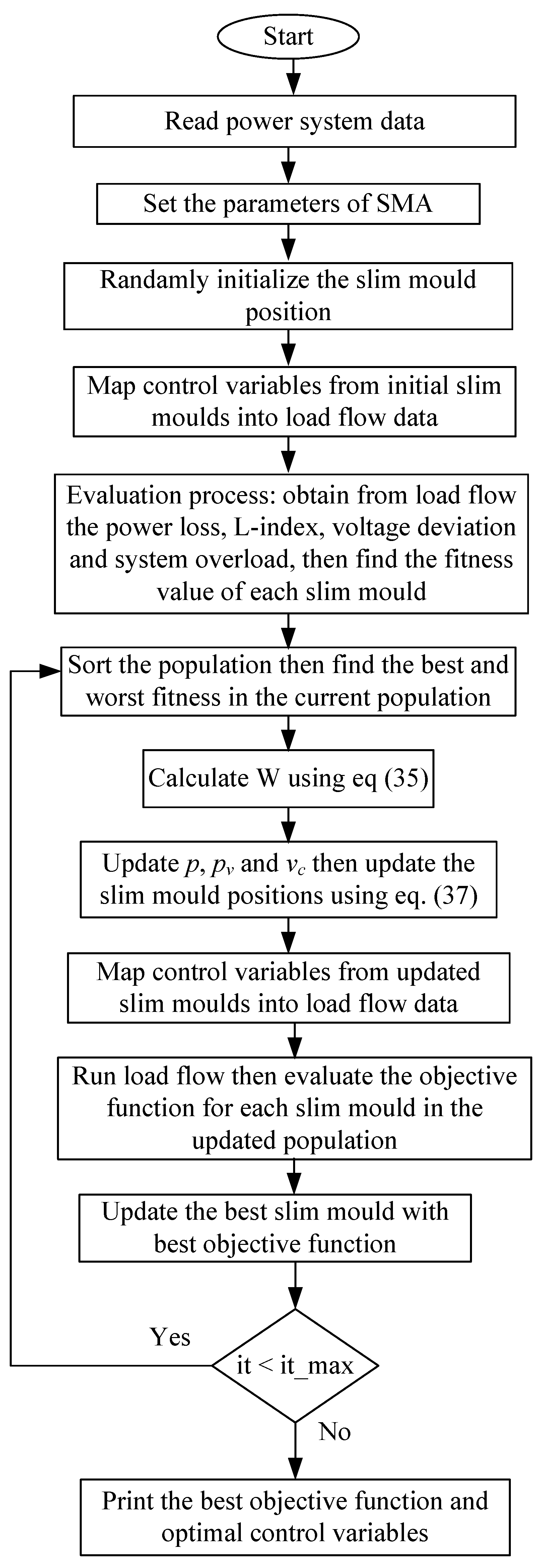
Algorithm 1 illustrates Pseudo-code of SMA [24]. More details about the SMA can be found in [24].

Algorithm 1: The pseudo-code of the slim mold algorithm (SMA) [24].

Initialization the parameters, population size, maximum iterations (max_it)

Initialization of slime mould’s positions $X_i$($i=1,2,\dots ,n$);

While (t ≤ max_it)

Compute the fitness of all slime mould.

Update bestFitness, $X_b$

Compute the W by Equation (35);

For each search section

Update p, vb, vc;

Update positions by Equation (37);

End For

$t=t+1$;

End While

ReturnbestFitness, $X_b$;

The main steps of the SMA for solving the ORPD problem can be summarized as follows:

• Step 1: Read the input data involving the power system structure, lines data, transformers data, shunt VAR compensators data, loads data, and generation unit’s data; specify the active power outputs of generators (except slack generator). Use the per-unit system.
• Step 2: Initialize the parameters of SMA, the population size, maximum iterations. Then initialize the slime mold’s positions.
• Step 3: The initial positions of each slim mold are arbitrarily chosen among lower and upper limits of the control variables.
• Step 4: Run the power flow program for each slim mold from the current population and determine the corresponding values of the objective function (fitness values).
• Step 5: Sort the population then obtain the best and worst fitness values in the current population.
• Step 6: Calculate W (the weight of slime mold) using Equation (35)
• Step 7: Update the parameters p, pv and vc then update the slim mold positions using Equation (37)
• Step 8: Run the power flow program for each slim mold from the new population and determine the corresponding values of the objective function.
• Step 9: Update the best slim mold with the best objective function.
• Step 10: Repeat steps 5–9 until the stop criterion (maximum number of iterations) is reached.
• Step 11: Print best solution found in the last iteration; Stop.

In addition, Figure 1 indicates the flowchart of SMA applied to obtain the optimal solution of the ORPD problem.

4. Simulation Results and Discussions

The SMA’s strength based on the developed objective function is illustrated based on two different IEEE systems. They are a 30-bus system and a 118-bus system. The proposed SMA technique along with the other compared algorithms has been run on an I7-8700 CPU, 2.8 GHz, 16 GB RAM PC and using MATLAB 2016a.

4.1. IEEE 30-Bus Test System

The IEEE 30-bus test system consists of six generators units located at buses 1, 2, 5, 8, 11, and 13, forty-one transmission lines, four regulating tap-changing transformers with off-nominal tap ratio at lines 4-12, 6-9, 6-10 and 28-27, and nine shunt VAR capacitors at the buses 10, 12, 15, 17, 20, 21, 23, 24, and 29. Furthermore, 24 load buses with 2.834 p.u. and 1.262 p.u. for both demand real and reactive power, respectively. The system data of the generator cost coefficients, the buses, lines, and the limits of the control and state variables are described in [31,32]. The boundary of voltage magnitude is considered between 0.95 and 1.1 p.u. for all generator buses. These limits are sited between 0.95 and 1.05 p.u. for all other buses. The output of nine shunt VAR capacitors varies between 0 and 0.05 p.u. and the transformer tap settings are settled to change within the range 0.9 and 1.1 p.u.

There are three cases in this system. In first case, there are 19 control variables considered for the ORPD problem: six voltage magnitudes of the generator, four transformer tap settings, and nine shunt VAR compensator reactive power injections. In the second and third cases, there are 25 control variables considered for the ORPD problem: six generator reactive power outputs, six voltage magnitudes of the generator, four transformer tap settings, and nine shunt VAR compensator reactive power injections.

The system is modified by incorporating RESs. The location of this RESs is selected according to minimizing both real power system loss and the cost of generating active and reactive power as introduced in [33]; however, the bus 30 was selected for adding RESs with a value of 20 MW.

4.1.1. First Case: Minimization of Real Power Loss for Base Case without (RESs)

The SMA technique is implemented on the IEEE 30-bus test system in order to minimize only the real power loss as a single objective function with the penalty terms corresponding to the constraints of the system. In this case, the considered control variables are six voltage of generators, four tap settings of transformer and nine shunt VAR reactive power compensators, which results in 19 control variables of the ORPD problem.

To display the superiority of the proposed SMA technique over other recent published techniques in solving the optimization problem of ORPD for minimizing real power loss, the optimal results are compared with the results of quasi-oppositional differential evolution (QODE) that presented in [34], PSO with an aging leader and challengers (ALC-PSO) [35], gravitational search algorithm (GSA) [36], opposition-based GSA (OGSA) [36], PSO-GSA [5], chaotic KHA (CKHA) [37], sine-cosine algorithm (SCA) [3], modified JAYA algorithm (MJAYA) [9], salp swarm algorithm (SSA) [38] and chaotic bat algorithm (CBA) [39].

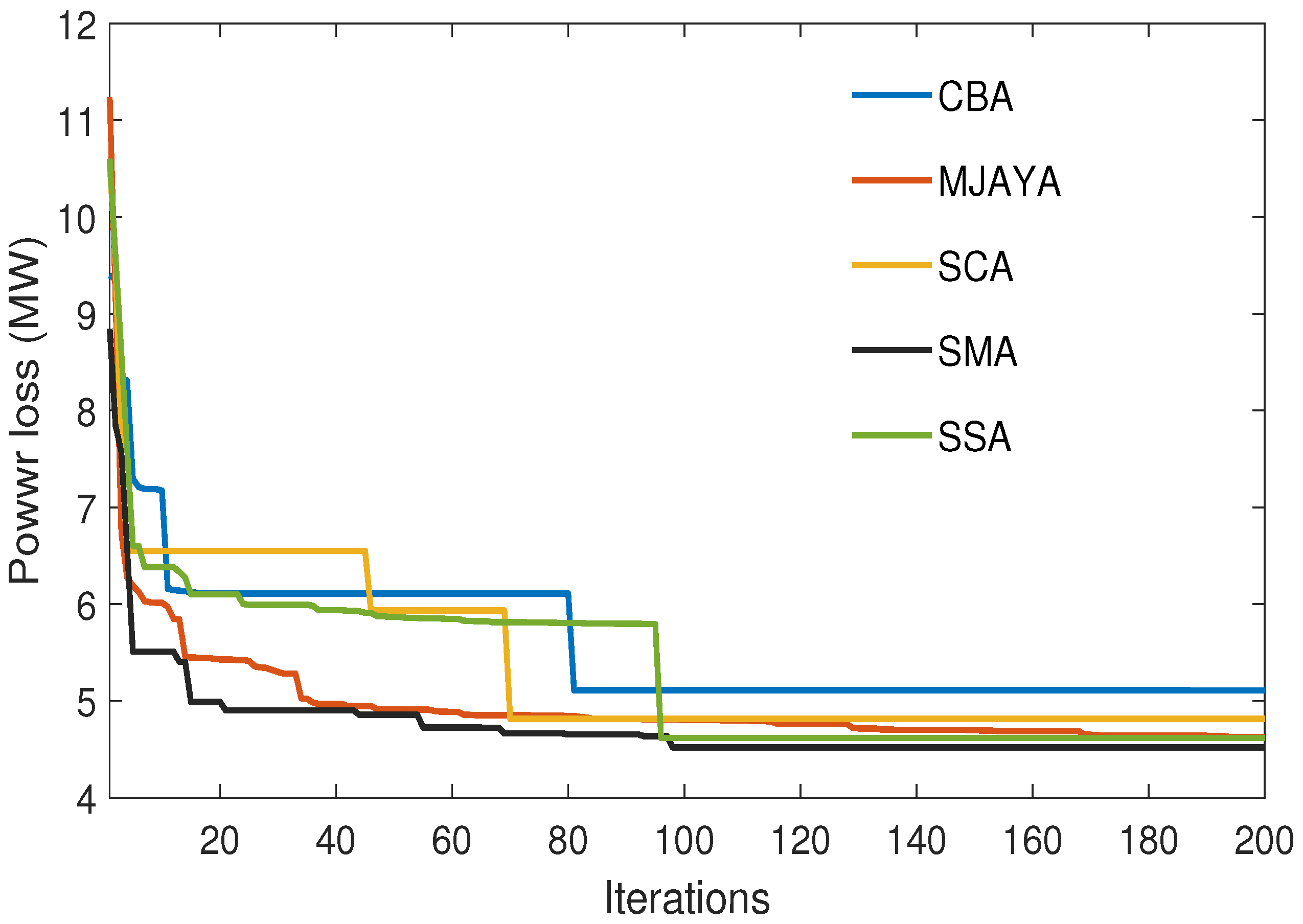
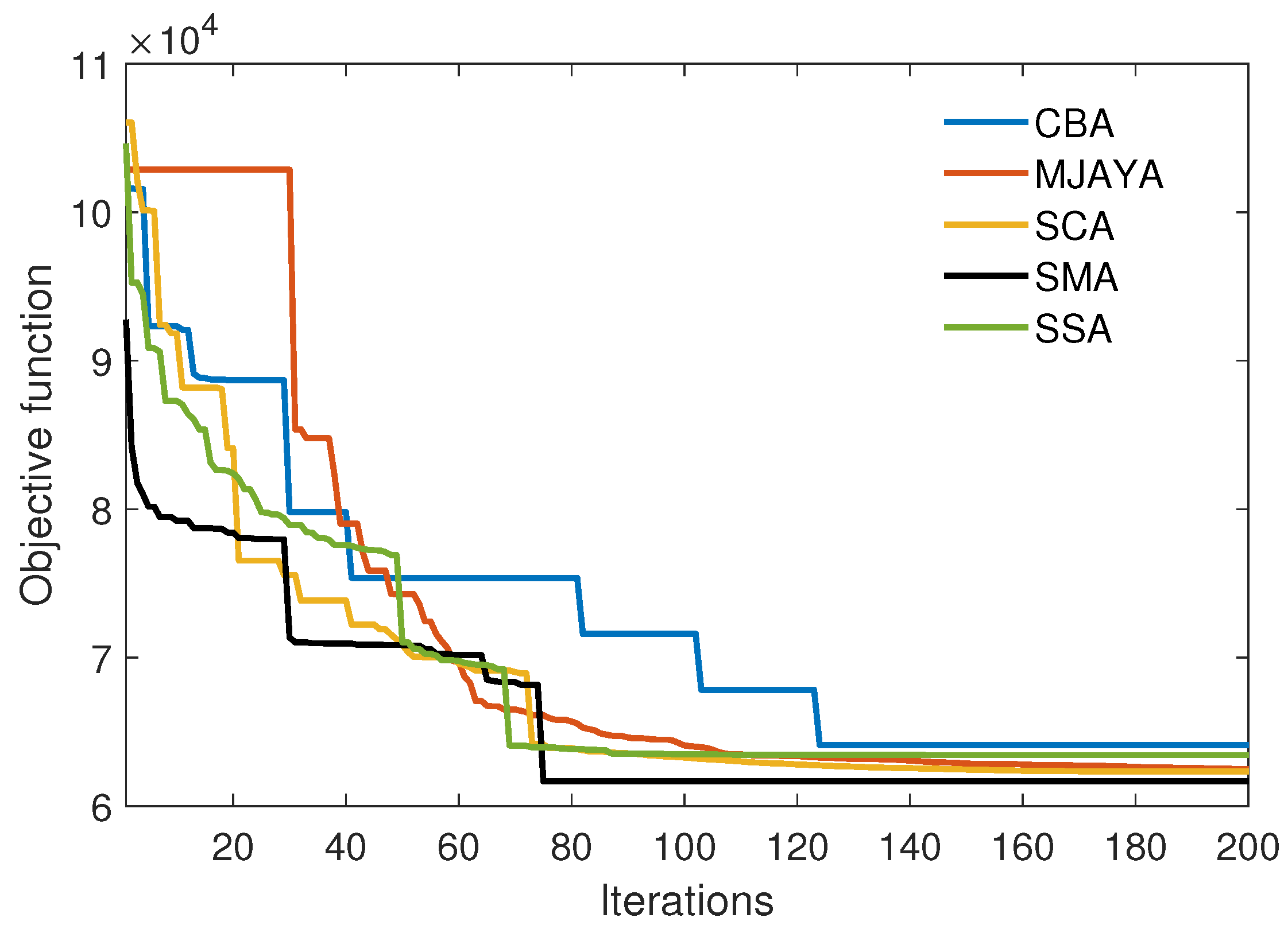
The values of real power loss for all compared techniques are given in

Table 1. Comparison of the objective function for first case.

Method	Power Loss (MW)
SCA	4.8139
MJAYA	4.6234
CBA	5.1081
SSA	4.559
CKHA [37]	5.1163
PSOGSA [40]	4.5309
QODE [34]	5.2953
ALC-PSO [35]	5.1861
OGSA [35]	5.1676
SMA	4.5181

. The real power loss corresponding to SMA is highly reduced by ($22.26\%$) compared to the base case. However, the percentage reduction in power loss compared to base case is $17.31\%$ by SCA, $20.58\%$ by MJAYA $20.72\%$ by SSA and $12.26\%$ by CBA. It is seen that the reduction of power loss using SMA has a higher percentage reduction in comparison with the other techniques with minimum computational time. Furthermore,

Table 2. OPRD results of the IEEE 30-Bus test System using SMA and other algorithms for first case.

	Base Case	SMA	SCA	MJAYA	SSA	CBA
$V_{G1}$ (p.u.)	1.0500	1.1000	1.1000	1.1000	1.1000	1.0451
$V_{G2}$ (p.u.)	1.0400	1.0950	1.0907	1.0919	1.0937	1.0376
$V_{G5}$ (p.u.)	1.0100	1.0749	1.0879	1.0670	1.0745	1.0138
$V_{G8}$ (p.u.)	1.0100	1.0763	1.0742	1.0698	1.0760	1.0158
$V_{G11}$ (p.u.)	1.0500	1.0974	1.1000	1.0953	1.1000	1.0764
$V_{G13}$ (p.u.)	1.0500	1.1000	1.1000	1.0684	1.0980	1.0374
$T_{11}$(6-9) (p.u.)	1.0780	0.9909	1.1000	0.9838	1.0234	0.9927
$T_{12}$(6-10) (p.u.)	1.0690	0.9827	1.0588	1.0350	0.9064	0.9754
$T_{15}$(4-12) (p.u.)	1.0320	1.0128	0.9000	1.0029	0.9779	0.9825
$T_{36}$(28-27) (p.u.)	1.0680	0.9801	1.1000	1.0009	0.9725	0.9625
$Q_{C10}$ (MVAR)	0.0000	0.5143	0.0000	4.9111	0.3382	4.9074
$Q_{C12}$ (MVAR)	0.0000	1.4536	0.3220	5.0000	4.3628	3.0239
$Q_{C15}$ (MVAR)	0.0000	0.6122	4.5128	5.0000	4.9891	3.3911
$Q_{C17}$ (MVAR)	0.0000	4.9797	0.0000	5.0000	4.4849	4.8860
$Q_{C20}$ (MVAR)	0.0000	3.4884	3.0436	4.3801	4.4474	4.2147
$Q_{C21}$ (MVAR)	0.0000	4.9841	1.8970	5.0000	5.0000	4.6343
$Q_{C23}$ (MVAR)	0.0000	4.9386	0.5739	4.0931	3.3318	4.6343
$Q_{C24}$ (MVAR)	0.0000	5.0000	4.1247	5.0000	4.9772	3.1860
$Q_{C29}$ (MVAR)	0.0000	2.3724	3.5914	4.7324	2.4617	2.1936
Real Power loss (MW)	5.8223	4.5181	4.8139	4.6235	4.6156	5.1081
Voltage deviation (p.u.)	1.1497	1.0659	1.0868	1.4218	1.9009	0.5129
Time (s)	—	59.0576	61.9849	64.3459	75.6574	80.1854

shows the results of optimal control variables for SMA compared with recent optimization techniques where the results offer that SMA gives better results than the SCA, MJAYA, SSA and CBA. According to convergence characteristics of compared optimization methods, as shown in Figure 2, the SMA has a smooth convergence curve without oscillations to the optimal value compared to other techniques.

Moreover, to enhance the efficiency of the SMA compared to recent optimization approaches. The statistical calculation is introduced in

Table 3. Comparison of the objective function of ORPD problem in first case.

Method	Maximum	Minimum	Average	SD
SMA	4.7814	4.5181	4.6300	0.0979
SCA	5.2896	4.8139	5.0258	0.1709
MJAYA	4.9991	4.6234	4.8183	0.1410
CBA	5.6234	5.1081	5.3972	0.1622
SSA	4.9519	4.5590	4.7697	0.1227

. The best results after 20 separate runs of SMA are compared with SCA, MJAYA, CBA, and SSA methods, where the minimum, maximum, average, and standard deviation (SD) values of all approaches are illustrated in the table. The results indicate that the new SMA has both better optimal solutions and minimum SD over other approaches.

4.1.2. Second Case: ORPD for IEEE 30-Bus System without (RESs)

The SMA technique is applied in this case without RESs to solve the ORPD problem considering the developed objective function act as CSOF for minimizing the total operating cost of system that consists of minimizing the cost of reactive power produced from generators and shunt VAR compensators, real power losses, voltage deviation, voltage stability index and system overload.

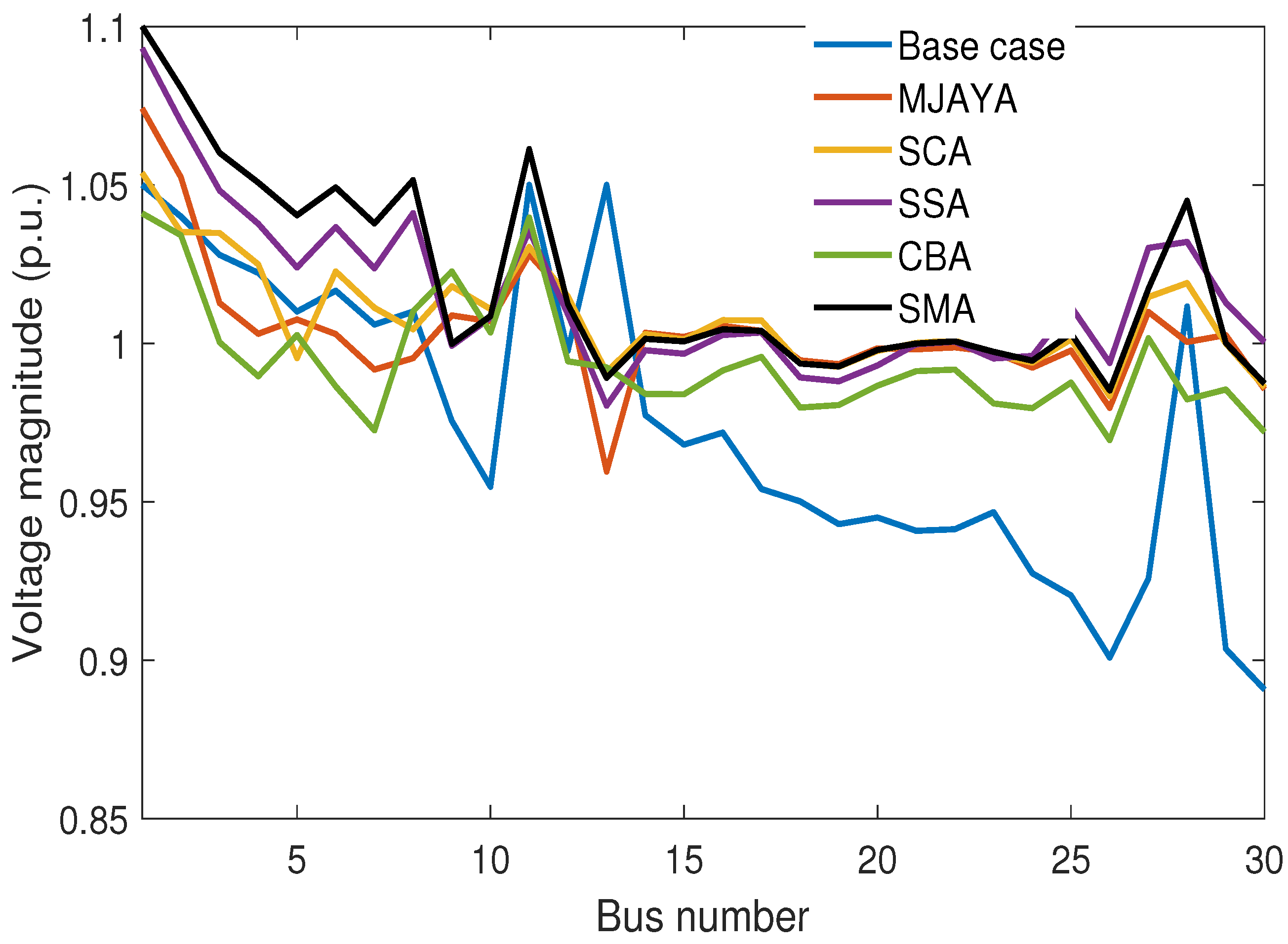
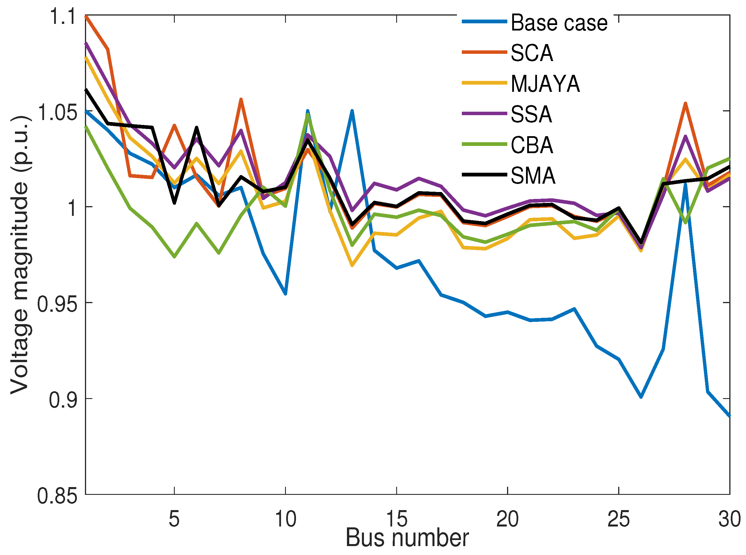
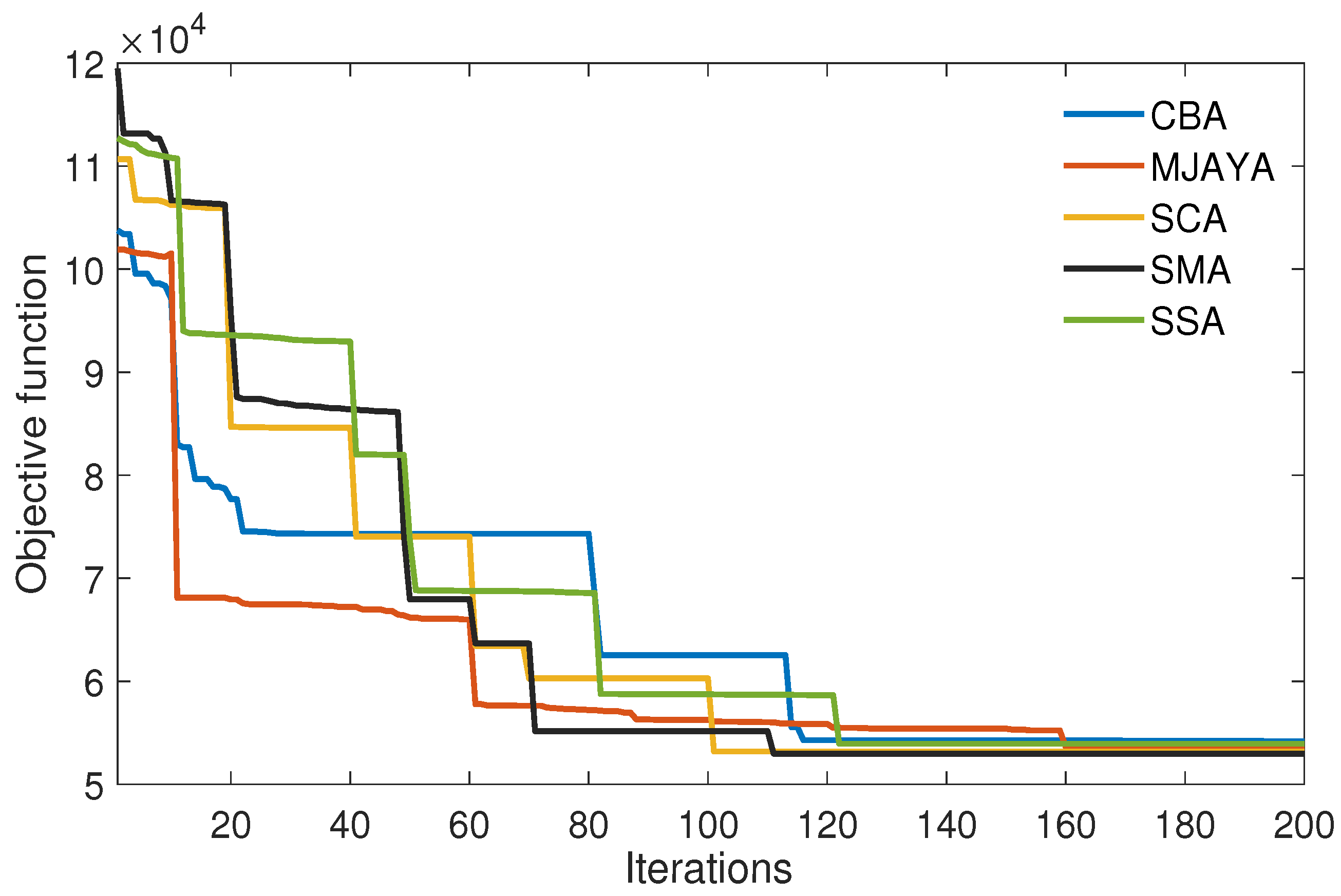
The simulation results of SMA are compared with the SCA, MJAYA, CBA and SSA techniques. The results are illustrated in

Table 4. OPRD results of IEEE 30-bus test system using SMA and other approaches for second case.

	Base Case	SMA	SCA	MJAYA	SSA	CBA
$Q_{G1}$ (MVAR)	−6.5435	27.0093	37.8328	25.0843	37.3283	42.1513
$Q_{G2}$ (MVAR)	15.6446	15.1664	32.3414	18.2873	13.8286	17.8375
$Q_{G5}$ (MVAR)	16.4069	8.6420	14.4327	11.3116	4.2513	11.8956
$Q_{G8}$ (MVAR)	13.5379	37.7084	13.5473	35.7144	45.8187	31.6733
$Q_{G11}$ (MVAR)	38.0025	14.2392	22.7156	11.0683	18.4888	16.5056
$Q_{G13}$ (MVAR)	39.5454	−17.1087	−18.7560	−16.4986	−19.8846	−17.2009
$V_{G1}$ (p.u.)	1.0500	1.1000	1.0741	1.0538	1.0931	1.0410
$V_{G2}$ (p.u.)	1.0400	1.0807	1.0524	1.0351	1.0699	1.0341
$V_{G5}$ (p.u.)	1.0100	1.0404	1.0075	0.9953	1.0239	1.0026
$V_{G8}$ (p.u.)	1.0100	1.0515	0.9953	1.0044	1.0411	1.0101
$V_{G11}$ (p.u.)	1.0500	1.0613	1.0280	1.0304	1.0355	1.0397
$V_{G13}$ (p.u.)	1.0500	0.9891	0.9595	0.9909	0.9803	0.9924
$T_{11}$(6-9) (p.u.)	1.0780	0.9936	1.0764	1.0097	1.0932	1.0028
$T_{12}$(6-10) (p.u.)	1.0690	1.0919	0.9251	0.9655	0.9118	0.9471
$T_{15}$(4-12) (p.u.)	1.0320	0.9771	0.9543	0.9238	0.9555	0.9500
$T_{36}$(28-27) (p.u.)	1.0680	1.0113	0.9071	0.9780	0.9679	0.9853
$Q_{C10}$ (MVAR)	0.0000	1.6608	3.9773	3.4391	0.7418	3.3003
$Q_{C12}$ (MVAR)	0.0000	4.7920	1.3894	0.0000	2.9311	2.9901
$Q_{C15}$ (MVAR)	0.0000	3.3921	1.5336	3.5544	2.2564	3.7044
$Q_{C17}$ (MVAR)	0.0000	5.0000	0.4726	5.0000	4.4348	3.7888
$Q_{C20}$ (MVAR)	0.0000	0.5249	4.2022	4.6573	0.6997	3.4575
$Q_{C21}$ (MVAR)	0.0000	4.9981	3.1834	5.0000	4.1474	3.9793
$Q_{C23}$ (MVAR)	0.0000	1.2935	4.4755	2.6146	0.7772	3.7729
$Q_{C24}$ (MVAR)	0.0000	4.9970	0.7068	5.0000	4.9811	3.0317
$Q_{C29}$ (MVAR)	0.0000	2.4218	1.9940	4.2960	0.2406	4.3759
Reactive power cost of generators (USD/h)	–	220.0514	220.1361	251.0970	292.5980	248.8023
Cost of shunt VAR compensators (USD/h)	–	5.5543	4.1896	6.4102	4.0511	6.1886
Real Power loss (MW)	5.8223	5.1128	5.4978	5.4742	5.4277	5.3364
Voltage deviation (p.u.)	1.1497	0.3013	0.3628	0.3526	0.3081	0.3466
L-index	0.3322	0.1008	0.1956	0.1409	0.1541	0.1006
System overload index	5.6951	4.2779	5.0722	4.3122	4.5417	4.5213
Total Objective function (USD/h)	–	527.5314	567.1370	586.0082	597.6855	612.1455
Time (s)	–	80.2390	86.9936	93.9515	89.6451	95.1444

. The results established that SMA outperforms other techniques. The SMA’s optimal value (527.5314 USD/h) is less than all tested techniques with no disruption of all constraints. Comparison of total system cost obtained from all compared techniques with SMA show increasing the system cost of $7.5077\%$ by SCA, $11.0849\%$ by MJAYA $13.2985\%$ by SSA and $16.0396\%$ by CBA. Voltage profiles of the SMA and other methods for all buses are presented in Figure 3. The figure shows that all magnitudes of the voltages are within the specified limits. However, the voltage profile in the case of using SMA has the better profile for the most buses of the system compared to other techniques.

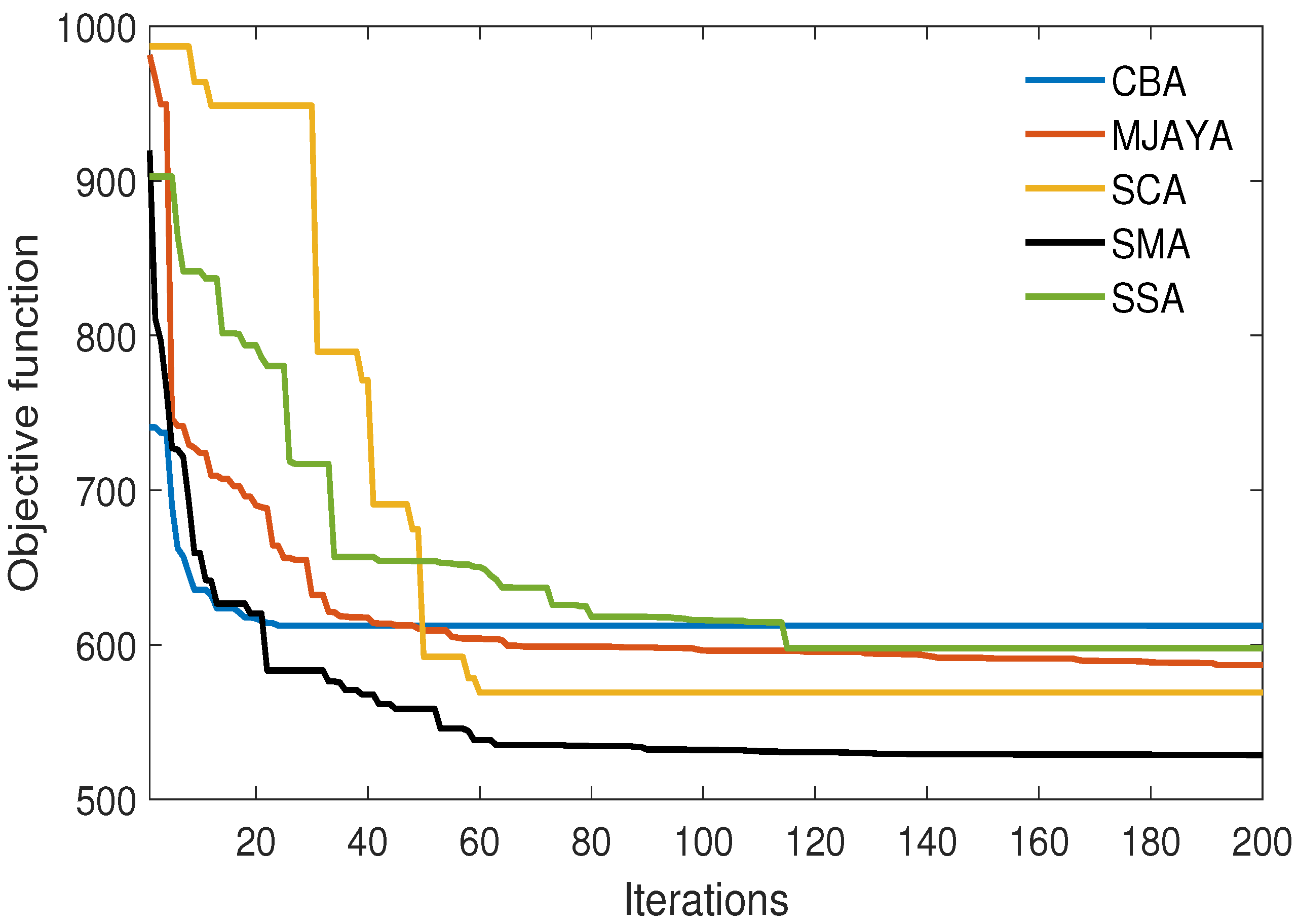
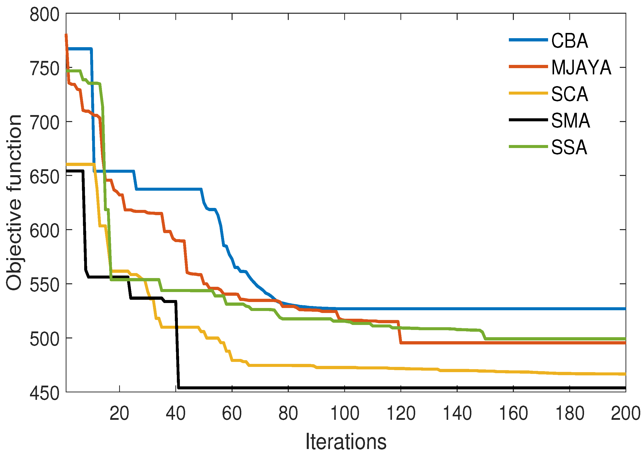
Based on the convergence curves of all approaches, which shown in Figure 4, the SMA offers a soft convergence curve to the optimal value of the objective function with no fluctuations. Moreover, the comparison of minimum, maximum, average, and SD of the obtained results using SMA, SCA, MJAYA, CBA, and SSA over 20 runs are offered in

Table 5. Comparison of the objective function of ORPD problem in second case.

Method	Maximum	Minimum	Average	SD
SMA	529.5092	527.5314	528.8728	0.4621
MJAYA	569.8306	567.1370	567.9265	1.4110
SCA	589.3406	586.0082	587.1010	1.1079
SSA	599.8354	597.6855	598.6409	0.8683
CBA	614.7140	612.1455	613.7493	0.8256

. From this table, it is seen that SMA offers the best values for minimum, average and SD values in comparison to SCA, MJAYA, SSA and CBA.

4.1.3. Third Case: ORPD for IEEE 30-Bus System with RESs

In this case, the SMA is used for solving the ORPD problem incorporating RESs based on developed objective function to minimize the system cost. The optimal results are obtained and compared with SCA, MJAYA, CBA, and SSA. The obtained results of the control variables for all techniques are given in

Table 6. OPRD solutions of the IEEE 30-bus system using SMA and other algorithms for third case.

	Base Case	SMA	SCA	MJAYA	SSA	CBA
$Q_{G1}$ (MVAR)	−6.5435	28.0509	28.2069	38.3354	37.6676	36.6650
$Q_{G2}$ (MVAR)	15.6446	16.8559	14.8075	10.6113	11.4282	11.5558
$Q_{G5}$ (MVAR)	16.4069	8.5213	8.0040	6.0654	4.6512	4.2198
$Q_{G8}$ (MVAR)	13.5379	37.2549	37.4778	41.6625	42.8978	42.5130
$Q_{G11}$ (MVAR)	38.0025	13.7881	12.4508	18.7964	16.9096	19.5375
$Q_{G13}$ (MVAR)	39.5454	−16.7981	−17.5558	−19.4119	−19.7736	−19.6198
$V_{G1}$ (p.u.)	1.0500	1.0613	1.0996	1.0781	1.0855	1.0420
$V_{G2}$ (p.u.)	1.0400	1.0434	1.0821	1.0561	1.0642	1.0201
$V_{G5}$ (p.u.)	1.0100	1.0020	1.0424	1.0123	1.0204	0.9740
$V_{G8}$ (p.u.)	1.0100	1.0156	1.0560	1.0290	1.0398	0.9956
$V_{G11}$ (p.u.)	1.0500	1.0348	1.0298	1.0363	1.0375	1.0481
$V_{G13}$ (p.u.)	1.0500	0.9908	0.9889	0.9695	0.9981	0.9800
$T_{11}$(6-9) (p.u.)	1.0780	1.0352	1.0800	1.0701	1.0809	0.9985
$T_{12}$(6-10) (p.u.)	1.0690	0.9159	0.9532	0.9000	0.9100	0.9454
$T_{15}$(4-12) (p.u.)	1.0320	0.9340	0.9678	0.9584	0.9252	0.9058
$T_{36}$(28-27) (p.u.)	1.0680	0.9922	1.0343	0.9961	1.0247	0.9675
$Q_{C10}$ (MVAR)	0.0000	1.6427	3.6694	0.0000	0.1242	2.1232
$Q_{C12}$ (MVAR)	0.0000	3.7694	2.4032	2.0113	2.6700	1.4961
$Q_{C15}$ (MVAR)	0.0000	1.6574	1.9694	1.4160	0.9073	2.0668
$Q_{C17}$ (MVAR)	0.0000	4.9995	4.9278	4.9441	4.9287	2.2025
$Q_{C20}$ (MVAR)	0.0000	1.9464	1.4500	0.0000	0.9067	0.5705
$Q_{C21}$ (MVAR)	0.0000	5.0000	5.0000	5.0000	4.5504	1.9537
$Q_{C23}$ (MVAR)	0.0000	0.7697	1.6645	1.6937	2.0589	3.7496
$Q_{C24}$ (MVAR)	0.0000	4.9850	5.0000	5.0000	4.7998	4.9414
$Q_{C29}$ (MVAR)	0.0000	1.4941	1.1385	0.0413	1.2406	2.4665
Reactive power cost of generators (USD/h)	–	225.1854	226.2213	275.8469	275.4956	278.2561
Cost of shunt VAR compensators (USD/h)	–	5.0165	5.2095	3.8403	4.2376	4.1199
Real power loss (MW)	5.8223	4.2590	4.3724	4.3583	4.3054	4.5750
Voltage deviation (p.u.)	1.1497	0.2142	0.4052	0.3334	0.3328	0.4536
L-index	0.3322	0.1129	0.1225	0.1566	0.1395	0.1593
System overload index	5.6951	4.0782	4.1936	4.2310	4.2634	4.3852
Total objective function (USD/h)	–	453.8077	467.2571	495.4014	499.1311	526.8994
Time (s)	–	81.2051	86.9936	93.9515	89.6451	95.1444

. The results show that SMA is further efficient than the tested approaches in obtaining the optimal solution of the ORPD problem including RESs. The minimum objective function using SMA has value of (453.8077 USD/h) that is better than all other techniques without violating the constraints.

From Table 6 it is seen that the total system operating cost of the compared techniques with SMA offer increasing the system cost of $2.9636\%$ by SCA, $9.1654\%$ by MJAYA, $9.9873\%$ by SSA, and $16.1063\%$ by CBA. Additionally, the entire SMA’s objective function is reduced from 527.5314 USD/h (second case) to 453.8077 USD/h in this case which shows the improvement of minimizing the developed objective function by 13.97% after incorporating the RESs. The RESs are connected to the system as a negative load; however the whole demand loads are decreased, which results in decreasing the developed objective function.

One can notice from Figure 5 the voltages’ magnitude of all buses fall within their limit and the improvement of the voltage profiles are proven based on the developed objective function. Additionally, Figure 6 clarifies the convergence characteristics of all techniques, showing that the SMA still has fast and smooth convergence characteristics compared with other methods. Finally, the statistical results are given in

Table 7. Comparison of the objective function of ORPD problem in third case.

Method	Maximum	Minimum	Average	SD
SMA	456.6274	453.8077	456.0750	0.6998
SCA	469.8147	466.6069	467.7170	1.1854
MJAYA	498.3406	495.4014	496.8934	1.0715
SSA	502.6855	499.1311	500.6563	1.0483
CBA	529.6108	526.8994	527.9883	0.9618

. As seen from this table, the SMA outperforms compared with other techniques, the SMA provides the lowest values of minimum, avearge and, SD values in comparison SCA, MJAYA, SSA, and CBA.

4.2. IEEE 118-Bus Test System

The IEEE 118-bus test system is employed as a large power system for evaluating the effectiveness of the SMA technique. This test system includes 186 transmission lines, 54 generators units where bus 69 is considered to be the slack bus, 14 shunt VAR compensators and 9 tap-changing transformers with off-nominal tap ratio [9,40,41,42]. Furthermore, 64 load buses with 42.42 p.u. and 14.38 p.u. for both demand real and reactive power, respectively. The initial real power loss is 1.3286 p.u. The buses, transmission lines, and cost coefficients data of the IEEE 118-bus test system are described in [41,42].

Moreover, the IEEE 118-bus test system contains 131 control variables: 54 reactive power generator, 54 bus generator voltages, 14 shunt VAR reactive power compensators, and 9 transformer tap settings. The limits of the voltage for all buses are within 0.94 and 1.06 p.u. The settings of the transformer tap are between the interval of 0.90 and 1.10 p.u. The shunt VAR available reactive powers within the interval 0–0.3 p.u. The standard test system is changed with incorporating RESs as found in [43]. RESs’ different technologies are located at buses 12, 31, 54, 76 and 116 with values of 0.182, 1.56, 2.64, 0.77 and 2.86 p.u., respectively.

4.2.1. Fourth Case: ORPD for IEEE 118-Bus System without RESs

For evaluating the scalability of the SMA and demonstrate its ability for dealing with the large-scale systems, the IEEE 118-bus system without considering the RESs is employed in this case.

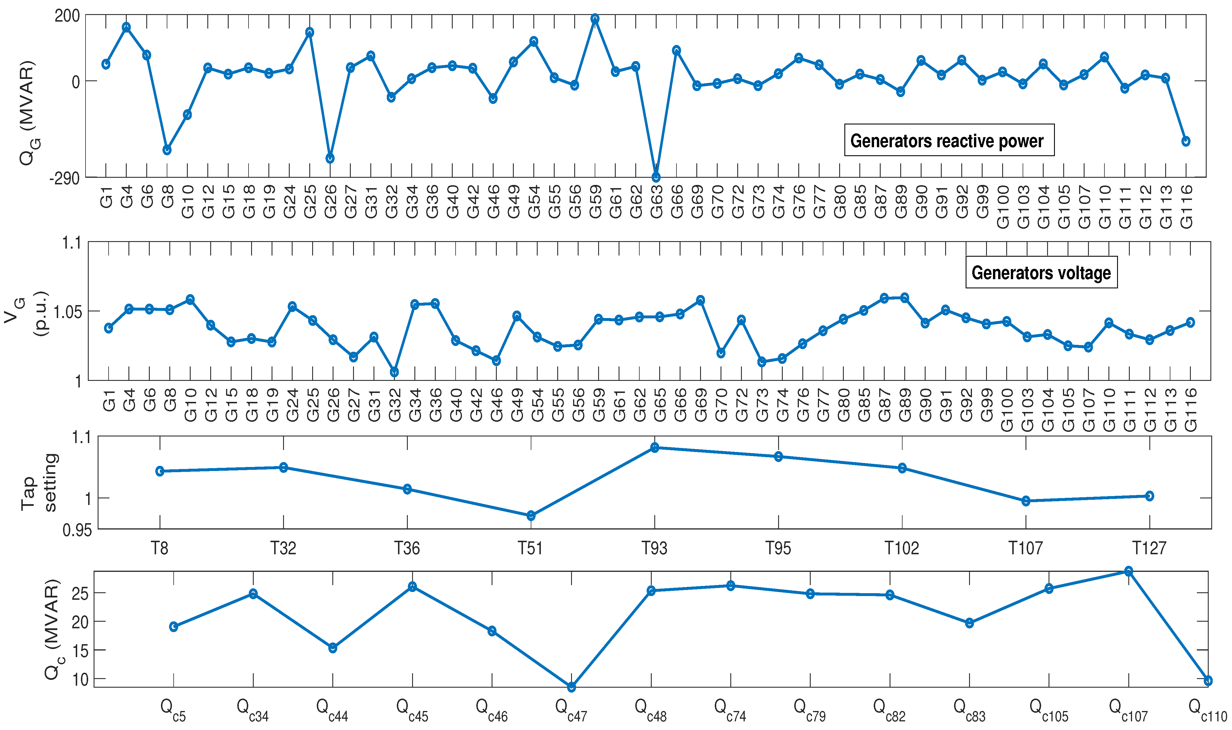
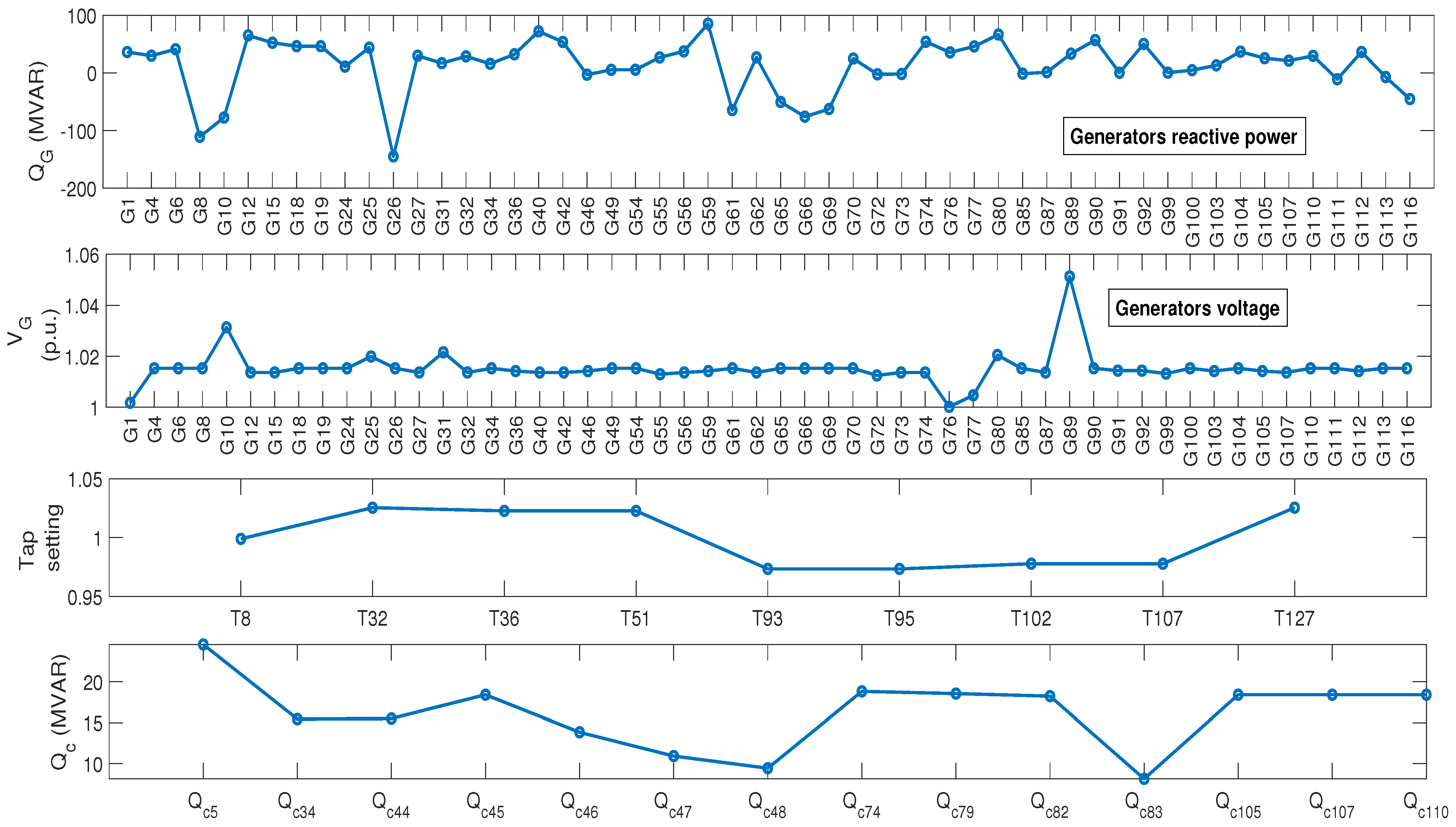
The optimal results of the developed objective function are obtained by SMA compared with other algorithms, and are tabulated in

Table 8. Objective function solutions of the IEEE 118-bus system for fourth case (without RESs).

	SMA	SCA	MJAYA	SSA	CBA
Reactive power cost of generators (USD/h)	21,871.91	23,793.23	24,720.88	22,371.51	27,183.79
Cost of shunt VAR compensators (USD/h)	36.25	37.15	37.17	39.12	38.55
Real power loss (MW)	120.65	124.51	125.96	126.15	124.23
Voltage deviation (p.u.)	0.72	0.79	2.03	1.31	0.77
L-index	1.06	1.07	2.03	1.85	0.77
System overload index	1.60	1.60	1.64	1.69	1.66
Total Objective function (USD/h)	61,678.98	62,330.16	62,503.73	63,454.71	64,108.04
Time (s)	354.82	357.87	361.17	374.25	387.87

.The control variables using SMA only are given in Figure 7 without violation the constraints.

According to the tabulated results, it can be noted that the SMA outperforms other methods as SMA gives a total system cost value 61,678.98 USD/h.

It is seen from Table 8, the total system cost of the compared techniques with SMA shows increasing the system cost of $1.0557\%$ by SCA, $1.3371\%$ by MJAYA, $2.8789\%$ by SSA, and $43.9382\%$ by CBA. Moreover, it is seen that SMA can minimize the total real power loss by $9.18\%$ compared to the initial case, which is better value than the real power loss achieved by the other techniques.

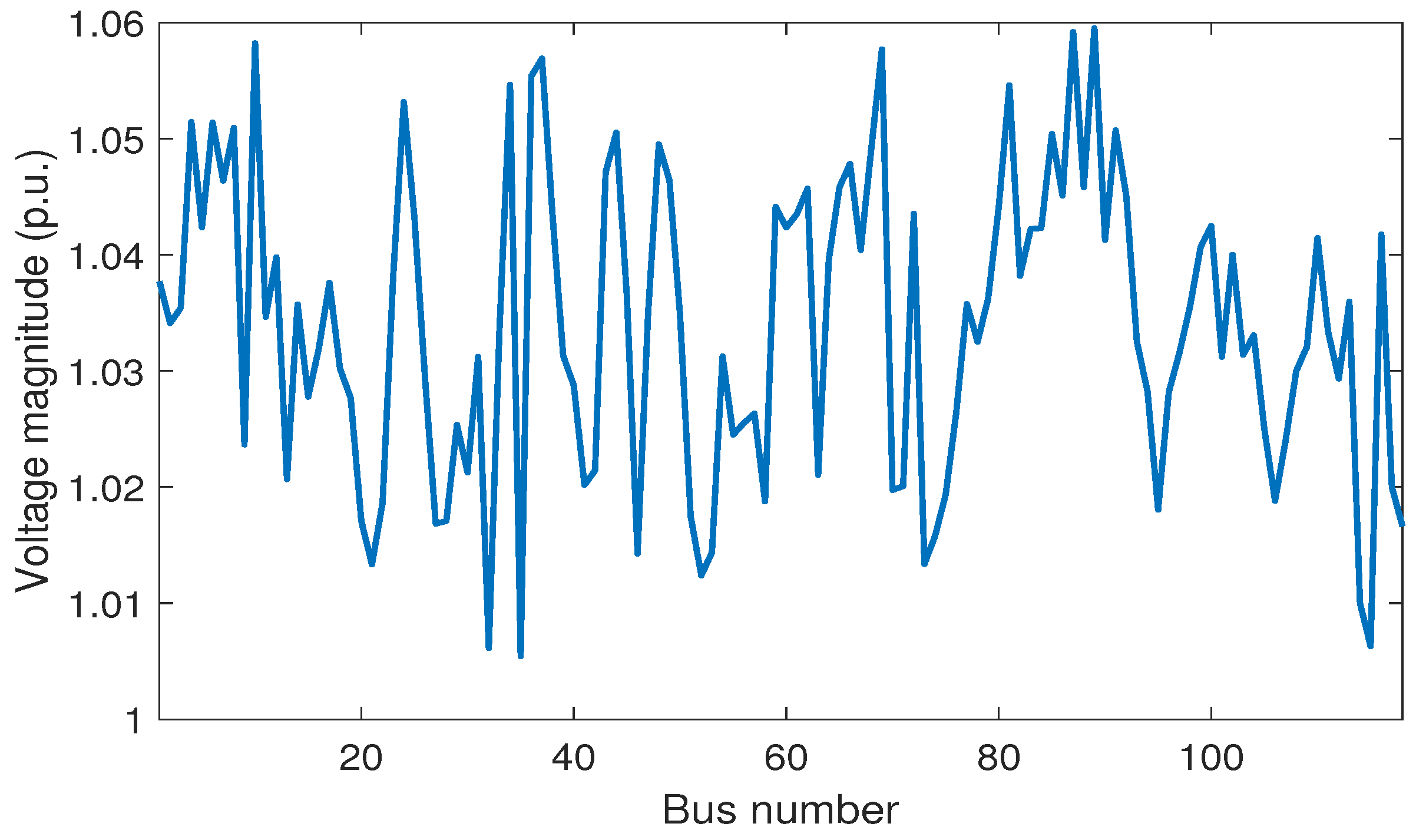
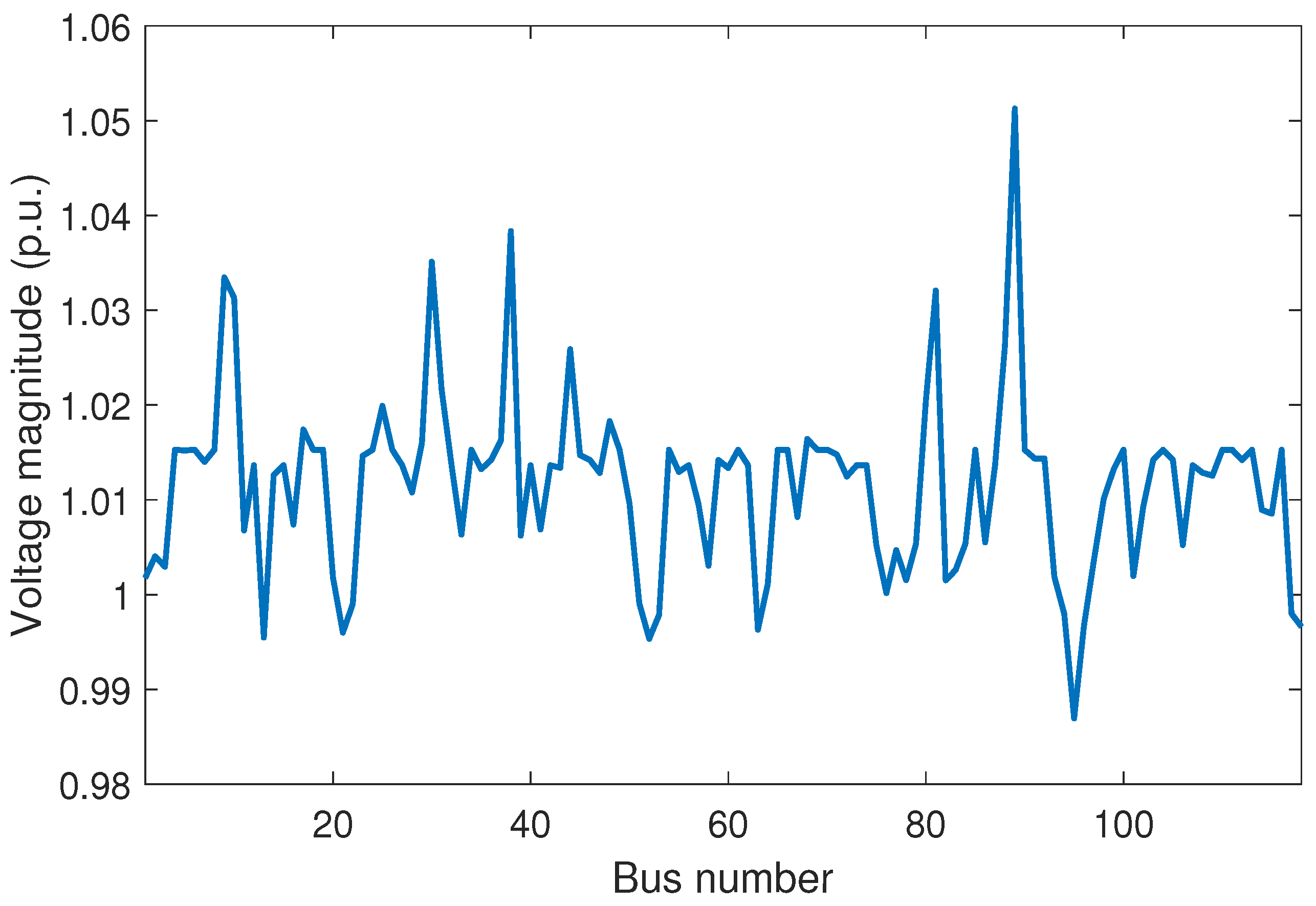
The magnitudes of voltages for all system’s buses based on SMA are inside borders, as shown in Figure 8. The comparative convergence curves of the considered objective function over 20 iterations for SMA and other compared techniques are shown in Figure 9. It confirms that the SMA yields better convergence than other algorithms.

4.2.2. Fifth Case: ORPD for IEEE 118-Bus System with RESs

The IEEE 118-bus system with RESs is considered in this case. The obtained results of the objective function by SMA and other techniques for this case are shown in

Table 9. Objective function solutions of IEEE 118-bus system for fifth case (considering RESs).

	SMA	SCA	MJAYA	SSA	CBA
Reactive power cost of generators (USD/h)	22,841.47	25,137.62	23,259.27	27,424.33	27,212.32
Cost of shunt VAR compensators (USD/h)	45.13	46.03	45.28	51.88	47.54
Real power loss (MW)	105.17	108.86	107.23	106.89	109.42
Voltage deviation (p.u.)	0.65	0.62	0.89	0.76	0.80
L-index	0.86	0.91	1.40	0.61	1.80
System overload index	1.59	1.61	1.62	1.59	1.78
Total objective function (USD/h)	52,830.01	53,189.12	53,627.65	53,943.78	54,220.47
Time (s)	345.60	352.19	372.19	381.77	403.91

. As seen from this table, the total operating cost of the compared techniques with SMA displays increasing the system cost of $0.6797\%$ by SCA, $1.5098\%$ by MJAYA, $2.1082\%$ by SSA, and $2.6319\%$ by CBA. These results indicate that the SMA gives a better optimal solution than other approaches in solving ORPD by considering RESs. Additionally, the obtained results of the control variables by SMA are given in Figure 10 without violating the considered constraints. It concluded that the total objective function is reduced by inserting RESs by $16.7498\%$ compared with fourth case (base case without RESs). Furthermore, the real power loss with considering RESs is reduced by $14.6334\%$ in comparison with fourth case. Moreover, the voltages of whole system buses of SMA are fall inside the borders as indicated in Figure 11. Once more, Figure 12 clear that the SMA has fast and smooth convergence behavior over other techniques.

4.3. Discussion

The obtained results from SMA are compared with other metaheuristic algorithms for five cases with and without RESs using two different test systems. These comparisons are indicated in Table 1, Table 2, Table 3, Table 4, Table 5, Table 6, Table 7, Table 8 and Table 9 and Figure 2, Figure 3, Figure 4, Figure 5, Figure 6, Figure 7, Figure 8, Figure 9, Figure 10, Figure 11 and Figure 12.

The first case is conducted to investigate the effectiveness of the SMA over other published algorithms in minimizing the real power loss only without RESs. Some of these algorithms are built by us while the remaining algorithms are built by other researchers. The second and third cases are conducted to investigate the superiority of the SMA over other recently published methods based on the developed objective function using the IEEE 30-bus without and with RESs, respectively. The fourth and fifth cases are conducted to investigate the superiority of the SMA over other algorithms based on the developed objective function using the IEEE 118-bus without and with RESs, respectively.

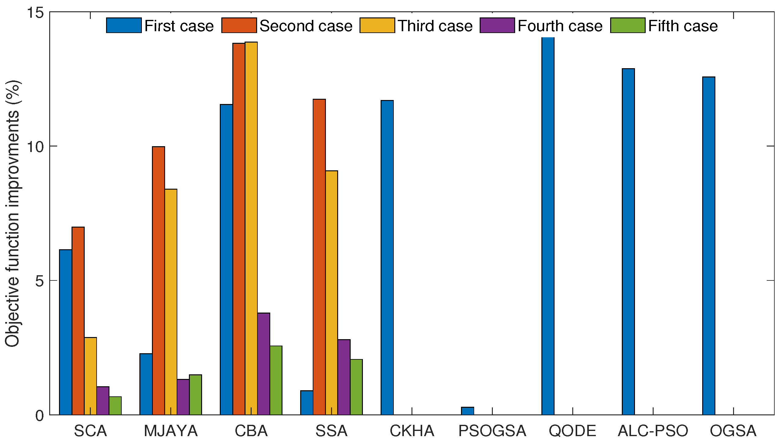
The results prove that the SMA can obtain better results in comparison with other methods for all cases. Figure 13 shows the objective function improvements of the SMA over other methods for all cases. It is well known that by expanding the dimensions of the test systems, the complexity of the ORPD problem increases due to its non-smooth and non-convex objective function. Consequently, the objective function of all algorithms increased with expanding the dimension of the system as shown in the above results. Moreover, the results show that the SMA obtains a better overall performance compared to other algorithms however the scale of the test system which demonstrates the capability of applying the SMA to solve the real applications of the ORPD problem.

The above results indicate that the SMA beats other published algorithms for all cases with or without RESs which demonstrates the capability of the SMA to obtain a better solution for different systems involving the large-scale test systems.

Figure 2, Figure 4, Figure 6, Figure 9 and Figure 12 illustrate the convergence characteristics of the objective function of the SMA and other algorithms of all cases. These results confirm that the objective function of the SMA converges smoothly to the optimal solution without any unexpected fluctuations in all cases. This indicates the convergence dependability of the SMA.

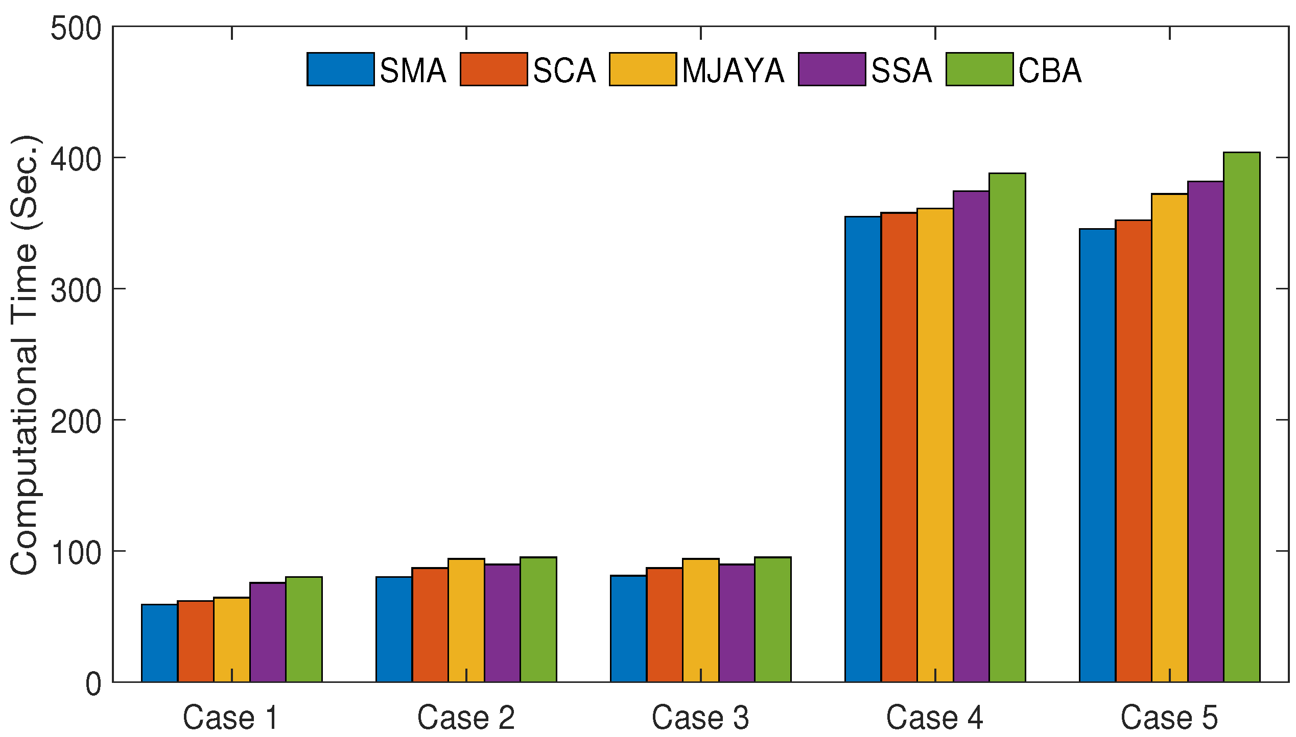
To fair comparison between different algorithms regarding the computational time, a similar computer configuration should be used. Therefore, Figure 14 illustrates the comparison between the SMA, SCA, MJAYA, SSA, and CBA algorithms for all cases. This figure indicates that the SMA has reasonable computational time (a few minutes for large-scale systems). Additionally, it has computational a little lower than other algorithms. This makes it feasible to use the SMA to obtain the optimal solution to the real-life ORPD problem.

In this work, 20 separate runs are performed to judge the robustness of the SMA. The results are shown in Table 3, Table 5 and Table 7. These results illustrate that the average and maximum values of the objective function achieved by the SMA are very close to their minimum values which prove the ability of the SMA to obtain either the optimum solution or very nearer to it in each run.

5. Conclusions

The application of SMA is successfully introduced to solve the OPRD problem in this work. A developed objective function to minimize the total operating cost of the system is presented as a multi-objective function then converted to CSOF using a price and penalty factors. This CSOF consists of minimization the reactive power cost generated from both generating units and shunt VAR compensators, total active power loss, voltage deviation, system overload, and voltage stability index. The advantage and superiority of the SMA have been confirmed using two standard test systems (IEEE 30 and 118 bus test system) based on different scenarios with and without inserting RESs. The results indicate that the SMA can obtain better results in comparison with other methods for all cases. It reduces the total objective function over other methods significantly. Additionally, the results confirm that the objective function of the SMA converges smoothly to the optimal solution without any fluctuation in all cases which proves that the SMA has reliable convergence characteristics. In addition, the ability of the SMA to obtain either the optimum solution or very nearer to it in each run in reasonable computational time is proven. Moreover, the scalability of the SMA is verified using a large-scale test system (IEEE 118-test system) which displays the ability of the SMA for solving real-life power system applications. In future work, the SMA could be used to solve the other complex problems in various fields such as optimal sizing and allocation of distributed generation, optimal modeling and planning of hybrid RES systems and estimation of the parameters of photovoltaic models, fuel cells, and many of electric machines and motors.

References

- Montoya, O.; Gonzalez, W.; Serra, F.; Hernandez, J.; Cabrera, A. A Second-Order Cone Programming Reformulation of the Economic Dispatch Problem of BESS for Apparent Power Compensation in AC Distribution Networks. Electronics 2020, 9, 1677. [Google Scholar] [CrossRef]
- Montoya, O.; Gonzalez, W.; Londono, A.; Rajagopalan, A.; Hernandez, J. Voltage Stability Analysis in Medium-Voltage Distribution Networks Using a Second-Order Cone Approximation. Energies 2020, 13, 5717. [Google Scholar] [CrossRef]
- Saddique, M.S.; Bhatti, A.R.; Haroon, S.S.; Sattar, M.K.; Amin, S.; Sajjad, I.A.; ul Haq, S.S.; Awan, A.B.; Rasheed, N. Solution to optimal reactive power dispatch in transmission system using meta-heuristic techniques:Status and technological review. Electr. Power Syst. Res. 2020, 178, 106031. [Google Scholar] [CrossRef]
- Aljohani, T.; Ebrahim, F.; Mohammed, O. Single and multiobjective optimal reactive power dispatch based on hybrid artificial physics particle swarm optimization. Energies 2019, 12, 2333. [Google Scholar] [CrossRef] [Green Version]
- Radosavljević, J.; Jevtić, M.; Milovanović, M. A solution to the ORPD problem and critical analysis of the results. Electr. Eng. 2018, 100, 253–265. [Google Scholar] [CrossRef]
- Karmakar, N.; Bhattacharyya, B. Optimal reactive power planning in power transmission network using sensitivity based bi-level strategy. Sustain. Energy Grids Netw. 2020, 23, 100383. [Google Scholar] [CrossRef]
- Soares, T.; Carvalho, L.; Morais, H.; Bessa, R.J.; Abreu, T.; Lambert, E. Reactive power provision by the DSO to the TSO considering renewable energy sources uncertainty. Sustain. Energy Grids Netw. 2020, 22, 10333. [Google Scholar] [CrossRef]
- Worighi, I.; Maach, A.; Hafid, A.; Hegazy, O.; Mierlo, J. Integrating renewable energy in smart grid system: Architecture, virtualization and analysis. Sustain. Energy Grids Netw. 2019, 18, 100226. [Google Scholar] [CrossRef]
- Elattar, E.; ElSayed, S. Modified JAYA algorithm for optimal power flow incorporating renewable energy sources considering the cost, emission, power loss and voltage profile improvement. Energy 2019, 178, 598–609. [Google Scholar] [CrossRef]
- Biswas, P.; Suganthan, P.; Mallipeddi, R.; Amaratunga, G. Optimal reactive power dispatch with uncertainties in load demand and renewable energy sources adopting scenario-based approach. Appl. Soft Comput. 2019, 75, 616–632. [Google Scholar] [CrossRef]
- Mehdinejad, M.; Ivatloo, B.; Bonab, R.; Zare, K. Solution of optimal reactive power dispatch of power systems using hybrid particle swarm optimization and imperialist competitive algorithms. Int. J. Electr. Power Energy Syst. 2016, 83, 104–116. [Google Scholar] [CrossRef]
- Jangir, P.; Parmar, A.; Trivedi, N.; Bhesdadiya, R. A novel hybrid particle swarm optimizer with multi verse optimizer for global numerical optimization and optimal reactive power dispatch problem. Eng. Sci. Technol. 2017, 20, 570–586. [Google Scholar] [CrossRef] [Green Version]
- Ramos, M.; Exposito, G.; Quintana, V. Transmission power loss reduction by interior-point methods: Implementation issues and practical experience. IEE Proc. Gener. Transm. Distrib. 2005, 152, 90–98. [Google Scholar] [CrossRef]
- Grudinin, N. Reactive power optimization using successive quadratic programming method. IEEE Trans. Power Syst. 1998, 13, 1219–1225. [Google Scholar] [CrossRef]
- Deeb, N.; Shahidehpour, S. An efficient technique for reactive power dispatch using a revised linear programming approach. Electr. Power Syst. Res. 1988, 15, 121–134. [Google Scholar] [CrossRef]
- Granada, M.; Rider, J.; Mantovani, J.; Shahidehpour, M. A decentralized approach for optimal reactive power dispatch using a Lagrangian decomposition method. Electr. Power Syst. Res. 2012, 89, 148–156. [Google Scholar] [CrossRef]
- Mei, R.; Sulaiman, M.; Mustaffa, Z.; Daniyal, H. Optimal reactive power dispatch solution by loss minimization using moth-flame optimization technique. Appl. Soft Comput. 2017, 59, 210–222. [Google Scholar]
- Dutta, S.; Mukhopadhyay, P.; Roy, P.; Nandi, D. Unified power flow controller based reactive power dispatch using oppositional krill herd algorithm. Int. J. Electr. Power Energy Syst. 2016, 80, 10–25. [Google Scholar] [CrossRef]
- Sulaiman, M.; Mustaffa, Z.; Mohamed, M.; Aliman, O. Using the gray wolf optimizer for solving optimal reactive power dispatch problem. Appl. Soft Comput. 2015, 32, 286–292. [Google Scholar] [CrossRef] [Green Version]
- Khazali, A.; Kalantar, M. Optimal reactive power dispatch based on harmony search algorithm. Int. J. Electr. Power Energy Syst. 2011, 33, 684–692. [Google Scholar] [CrossRef]
- Li, Y.; Li, X.; Zongpu, Z.L. Reactive power optimization using hybrid CABC-DE algorithm. Electr. Power Components Syst. 2017, 45, 980–989. [Google Scholar] [CrossRef]
- Heidari, A.; Abbaspour, R.; Jordehi, A. Gaussian bare-bones water cycle algorithm for optimal reactive power dispatch in electrical power systems. Appl. Soft Comput. 2017, 57, 657–671. [Google Scholar] [CrossRef]
- Naderi, E.; Narimani, H.; Fathi, M.; Narimani, M. A novel fuzzy adaptive configuration of particle swarm optimization to solve large-scale optimal reactive power dispatch. Appl. Soft Comput. 2017, 53, 441–456. [Google Scholar] [CrossRef]
- Li, S.; Chen, H.; Wang, M.; Heidari, A.A.; Mirjalili, S. Slime mould algorithm: A new method for stochastic optimization. Future Gener. Comput. Syst. 2020, 11, 300–323. [Google Scholar] [CrossRef]
- Ketabi, A.; Alibabaee, A.; Feuillet, R. Application of the ant colony search algorithm to reactive power pricing in an open electricity market. Int. J. Electr. Power Energy Syst. 2010, 32, 622–628. [Google Scholar] [CrossRef]
- De, M.; Goswami, S. Reactive power cost allocation by power tracing based method. Energy Convers. Manag. 2012, 64, 43–51. [Google Scholar] [CrossRef]
- Malakar, T.; Goswami, S. Active and reactive dispatch with minimum control movements. Int. J. Electr. Power Energy Syst. 2013, 44, 78–87. [Google Scholar] [CrossRef]
- Rojas, D.; Lezama, J.; Villa, W. Metaheuristic techniques applied to the optimal reactive power dispatch: A review. IEEE Lat. Am. Trans. 2016, 14, 2253–2263. [Google Scholar] [CrossRef]
- Mouassa, S.; Bouktir, T.; Salhi, A. Ant lion optimizer for solving optimal reactive power dispatch problem in power systems. Eng. Sci. Technol. Int. J. 2017, 20, 885–895. [Google Scholar] [CrossRef]
- Sahli, Z.; Hamouda, A.; Bekrar, A.; Trentesaux, D. Reactive power dispatch optimization with voltage profile improvement using an efficient hybrid algorithm. Energies 2018, 11, 2134. [Google Scholar] [CrossRef] [Green Version]
- Lee, K.; Park, Y.; Ortiz, J. A united approach to optimal real and reactive power dispatch. IEEE Trans. Power Appar. Syst. 1985, 5, 1147–1153. [Google Scholar] [CrossRef]
- Duman, S.; Sönmez, Y.; Güvenç, U.; Yörükeren, N. Optimal reactive power dispatch using a gravitational search algorithm. IET Gener. Transm. Distrib. 2012, 6, 563–576. [Google Scholar] [CrossRef]
- Warid, W.; Hizamm, H.; Mariun, N.; Abdul-Wahab, N. Optimal power flow using the Jaya algorithm. Energies 2016, 9, 678. [Google Scholar] [CrossRef]
- Basu, M. Quasi-oppositional differential evolution for optimal reactive power dispatch. Int. J. Electr. Power Energy Syst. 2016, 78, 29–40. [Google Scholar] [CrossRef]
- Singh, R.; Mukherjee, V.; Ghoshal, S. Optimal reactive power dispatch by particle swarm optimization with an aging leader and challengers. Appl. Soft Comput. 2015, 29, 298–309. [Google Scholar] [CrossRef]
- Shaw, B.; Mukherjee, V.; Ghoshal, S. Solution of reactive power dispatch of power systems by an opposition-based gravitational search algorithm. Int. J. Electr. Power Energy Syst. 2014, 55, 29–40. [Google Scholar] [CrossRef] [Green Version]
- Mukherjee, A.; Mukherjee, V. Solution of optimal reactive power dispatch by chaotic krill herd algorithm. IET Gener. Transm. Distrib. 2015, 9, 2351–2362. [Google Scholar] [CrossRef]
- Elattar, E.; ElSayed, S. Probabilistic energy management with emission of renewable micro-grids including storage devices based on efficient salp swarm algorithm. Renew. Energy 2020, 153, 23–35. [Google Scholar] [CrossRef]
- Mugemanyi, S.; Qu, Z.; Rugema, F.X.; Dong, Y.; Bananeza, C.; Wang, L. Optimal Reactive Power Dispatch Using Chaotic Bat Algorithm. IEEE Access 2020, 8, 65830–65867. [Google Scholar] [CrossRef]
- Radosavljevic, J. Metaheuristic Optimization in Power Engineering; The Institution of Engineering and Technology (IET): London, UK, 2018. [Google Scholar]
- Washington University Website. IEEE Test Systems Data. Available online: www.ee.washington.edu/research/pstca/ (accessed on 10 June 2020).
- Matpower. Matpower Matlab Toolbox. Available online: http://www.pserc.cornell.edu/matpower (accessed on 10 June 2020).
- Pena, I.; Martinez-Anido, C.; Hodge, B. An extended IEEE 118-bus test system with high renewable penetration. IEEE Trans. Power Syst. 2017, 33, 281–289. [Google Scholar] [CrossRef]
Figure 1.
Flowchart of the SMA applied to solve the ORPD problem.
Figure 2.
Convergence characteristic of all methods for first case.
Figure 3.
Voltage magnitude of compared approaches in the second case.
Figure 4.
Convergence characteristic of all methods for second case.
Figure 5.
Voltage magnitude of compared approaches in third case.
Figure 6.
Convergence characteristic of all methods for third case.
Figure 7.
OPRD results of the IEEE 118-bus system using SMA for fourth case.
Figure 8.
Voltage magnitude of compared approaches in fourth case.
Figure 9.
Convergence characteristic of whole approaches for fourth case.
Figure 10.
OPRD results of IEEE 118-bus test system using SMA for fifth case.
Figure 11.
Voltage profile of the SMA for fifth case.
Figure 12.
Convergence characteristic of all methods for fifth case.
Figure 13.
The objective function improvements of SMA over other methods for all cases.
Figure 14.
The computational time of all methods for all cases.