
Sustainable Performance Analysis of Power Supply Chain System from the Perspective of Technology and Management

1
School of Business and Dongwu Think Tank, Soochow University, Suzhou 215021, China
2
Department of Finance and Business Management, International College, Renmin University of China, Beijing 100872, China
3
Centre of Chinese Urbanization Studies & School of Business, Soochow University, Suzhou 215012, China
*
Author to whom correspondence should be addressed.
Sustainability 2021, 13(11), 5972; https://0-doi-org.brum.beds.ac.uk/10.3390/su13115972
Submission received: 4 April 2021
/
Revised: 10 May 2021
/
Accepted: 14 May 2021
/
Published: 26 May 2021
(This article belongs to the Special Issue Sustainable Supply Chain and Logistics Management in a Digital Age)
Abstract
:The power industry is an important strategic industry that has effectively advanced the rapid development of China’s economy. However, this rapid development has created significant environmental problems and does not support the sustainable development of the ecological environment and economy. This study evaluated and analyzed the sustainable performance of China’s inter-provincial power supply chain systems (PSCSs), and developed policy recommendations for further developing China’s power industry based on the research results. For PSCSs with internal subsystems, this study first developed a non-radial two-stage model, and proposed steps to solve the model; then, this study applied the proposed model to empirically analyze China’s inter-provincial PSCSs. The empirical analysis yielded the following key research findings. Firstly, for the study period, China’s power industry had a low overall performance, and PSCS performance varied significantly across different regions. Secondly, the average meta-frontier efficiency (ME) of PSCSs in high-income regions was the highest; the average ME of PSCSs in middle-income regions was the lowest. This is consistent with the environmental Kuznets curve hypothesis. Thirdly, this study found that the PSCSs had effective management and technical systems in Qinghai and Guangdong. The PSCSs in other regions need improvements to mitigate either inadequate management, inadequate technology, or both.
1. Introduction
The power industry has played a significant role in advancing China’s economic development [1]. However, the rapid development of the industry has highlighted the visibility of conflicts between power generation and ecological environment protection [2,3]. For example, coal-fired power plants emit large quantities of greenhouse gases, which are associated with climate change [4]. As the power supply chain system (PSCS) is an important part of the industrial base, and is a major carbon emitter in China, its sustainable development is a key way to conserve energy and reduce emissions [5].
A PSCS mainly includes a power generation subsystem (PG) and a power grid subsystem (PGS) [6]. The PG is responsible for power production, and the PGS is responsible for power transportation, power distribution and power retail [7]. Improving the overall efficiency of the PSCS requires the joint efforts of all subsystems within the supply chain [8].
Studies have been conducted to assess PSCS performance; however, there are some current research gaps. Firstly, most previous studies focused on assessing PSCS performance, but only a few studies have analyzed the potential causes of PSCS inefficiency [6]. This makes it difficult to make recommendations on the direction of performance improvements. Secondly, most previous studies have evaluated the efficiency of the entire power industry or power companies, but have not assessed the internal subsystems of the PSCS. This may lead to an overestimate of PSCS performance.
This study proposed a new performance model for PSCSs and applied it to analyze the performance of China’s regional PSCSs. This study specifically answered the following research questions. First, how can the performance of PSCSs be modeled by considering internal subsystems? Second, how can the problem of overestimating PSCS performance be avoided? Third, how does the disposable income of residents affect the environmental performance of the regional PSCSs? Fourth, how can China’s regional PSCSs improve their performance?
This study makes three main theoretical contributions to the field. The first is that this study classified regional PSCSs in China based on the level of residents’ disposable income, and analyzed the impact of that income on regional PSCS performance. The second is that this study introduced a non-radial directional distance function (DDF) into the data envelopment analysis (DEA) model. Compared with previous models (e.g., [9]), this study’s model effectively avoids the problem of overestimating performance. The third is that, in addition to the performance evaluation model, this study further deconstructed the inefficiencies into management inefficiency and technical inefficiency, and provided specific recommendations for inefficient PSCSs.
In addition to the above theoretical contributions, this study also yielded key research findings. First, China’s overall PSCS performance during the study period was low, with significant opportunities for improvement. In addition, there were significant differences in PSCS performance between different regions. Second, the PSCSs in the high-income regions had the highest average meta-frontier efficiency (ME); PSCSs in the middle-income regions had the lowest ME. This result is consistent with the environmental Kuznets curve hypothesis. Third, this study found that only the PSCSs in Qinghai and Guangdong performed well with respect to both management and technological potential. The PSCSs in other regions need to correct either management insufficiencies, technical insufficiencies, or both.
The rest of this paper is organized as follows. Section 2 reviews the relevant research literature. Section 3 proposes the non-radial PSCS performance evaluation models. Section 4 applies the model of this study to empirically analyze PSCSs in China. Section 5 summarizes the study and proposes policy recommendations.
2. Literature Review
There are three main literature streams related to this research topic: (1) performance evaluations of the power industry without regarding environmental factors, (2) evaluations of environmental efficiencies in the power industry, (3) research using a two-stage DEA model, and (4) the relationship between environmental performance and economic income. This section summarizes these areas.
2.1. Performance Evaluation for the Power Industry without Environmental Factors
As an effective non-parametric mathematical programming method, DEA has many advantages. For example, it does not need to assume the functional relationship between input and output, and does not need to pre-determine weights [10]. Therefore, DEA can objectively evaluate the input-output efficiency of the decision-making unit. In view of the importance of the power industry in the national economy, many studies have evaluated the performance of the power industry by using DEA models. Färe et al. [11] applied DEA to assess PSCS performance, and compared the performance of public and private companies. Golany et al. [12] employed DEA to measure power-plant performance in the Israeli Electric Corporation. Sueyoshi and Goto [13] proposed an adjusted DEA model to examine the performance of Japanese power generation enterprises from 1984 to 1993. That study also included specific recommendations for the development of the Japanese power industry. Arocena [14] applied DEA to analyze the vertical integration, diversification, and economies of scale within the Spanish power industry. That study concluded that the largest utilities could improve their efficiencies of scale by dividing them into smaller units. Sueyoshi and Goto [15] used DEA to classify energy companies into efficient and non-efficient categories, and then developed an improved DEA method to rank energy companies. Xin-Gang and Zhen [16] adopted a four-stage DEA method to measure and analyze the technical efficiency of China’s wind power enterprises. That study found that the overall efficiency of China’s wind power industry was low from 2011 to 2015.
2.2. Environmental Performance of Power Industry
The rapid development of the power industry has led to significant environmental problems. Scholars have realized that it is not enough to evaluate the performance of the power industry from the perspective of economic output. This has led to increased scholarly interest in evaluating the environmental performance of the power industry by using DEA models. Zhou et al. [1] combined the entropy model and the DEA model to propose an improved non-radial method for evaluating the environmental efficiency of the Chinese provincial power industry. The results found significant differences in the environmental efficiencies between provincial power systems in China. Zhang et al. [17] proposed two non-radial DEA methods to analyze the carbon efficiency of fossil fuel power plants, which revealed a significant positive correlation between plant size and efficiency. Chen et al. [18] applied a game-based cross-efficiency model to analyze China’s provincial power efficiency. The results showed that China’s provincial power efficiency has not improved significantly from 2005 to 2014.
Wang et al. [19] applied several DEA methods to analyze the operation and environmental performance of China’s provincial thermal power industry, and then used the Malmquist index to analyze the dynamic performance changes. Sartori et al. [20] used DDF-DEA to evaluate the sustainable development of the Brazilian power industry using five scenarios. The results showed that the company’s performance differed under different application scenarios. Chen et al. [21] proposed a DEA model to analyze the energy congestion in China’s regional coal-fired power generation industry. Energy congestion means low energy efficiency, which is specifically defined as “reducing energy input will lead to an increase in one or more outputs without worsening other inputs or outputs” [21,22,23]. The empirical analysis showed that the coal-fired power industry faces undesirable energy congestion problems in the most underdeveloped areas of China. Undesired energy congestion is defined as “increasing input will cause a decrease in desired output” [21].
2.3. Two-Stage DEA Model
This study developed a two-stage non-radial model to study the performance of China’s PSCSs. As such, it is important to review relevant literature about the two-stage DEA model. As the research has deepened, scholars have found that the traditional single-stage DEA model does not effectively describe actual production processes. This led to the development of two-stage DEA models. Seiford and Zhu [24] applied the DEA model to evaluate the profitability and market efficiency of the United States commercial banks. Kao and Hwang [25] improved the traditional DEA model into a two-stage DEA model to measure the efficiency of the entire decision-making process and each decision-making stage. Chen et al. [26] extended Kao and Hwang’s model [25], proposing an additive two-stage DEA model, which broke down the overall efficiency of the system into a weighted sum of the efficiency of all stages.
Wang et al. [27] proposed a two-stage weighted DEA model to evaluate the efficiency of systems with shared inputs, and analyzed the relationship between weights, system efficiency, and subsystem efficiency. Zhu et al. [28] used a two-stage DEA resource allocation method, considered the fixed cost as a shared input for two stages in the decision-making unit, and designed three resource allocation schemes. Chu et al. [29] applied a two-stage non-cooperative DEA resource allocation method. The study concluded that the method ensured the uniqueness of the resource allocation scheme.
Sun et al. [30] adopted a two-stage game-based DEA model to evaluate the performance of circular economy systems. The model used considered the game relationship between the subsystems, and effectively identified the technical gaps between the systems. Sun et al. [6] proposed a two-stage DEA model to analyze the sustainable performance of a power system. The proposed model considered the non-cooperative relationship between power subsystems. Yin et al. [31] employed a bi-target two-stage DEA model from the perspective of cooperation. Solving the model included designing a new algorithm.
2.4. The Relationship between Environmental Performance and Economic Income
Some scholars have also analyzed the relationship between economic development and environmental performance. For example, Taskin and Zaim [32] analyzed the impact of per capita income and international trade factors on environmental efficiency. The results demonstrate that per capita income and environmental performance show a relationship of the environmental Kuznets curve type. Halkos and Tzeremes [33] first used the window DEA method to evaluate the environmental performance of 17 OECD countries, and then verified the Kuznets relationship between environmental performance and national income through the generalized moment estimation method. The results show that there is no U-shaped relationship between environmental efficiency and per capita income. Wang [34] used the non-radial DEA method to analyze the energy-saving and emission reduction performance of 209 cities in China, and found that there is a U-shape between energy-saving and emission reduction performance and income. Halkos and Polemis [35] used the DEA method to evaluate the environmental performance of the US power generation industry, and studied the relationship between environmental performance and economic development. The results show that in the global context, environmental efficiency and regional economic growth have a stable N-shaped relationship.
2.5. Literature Summary
The literature shows that PSCS performance has attracted scholarly attention, with DEA methods being increasingly used to evaluate PSCS performance. This study differs from these previous studies in two key ways. First, this study introduces Kuosmanen’s technique [36] and the non-radial method to the two-stage DEA model to solve the problem of overestimating efficiencies. Second, this study further explores the impact of residents’ income on PSCS performance.
3. Methodology
3.1. Traditional DDF Model
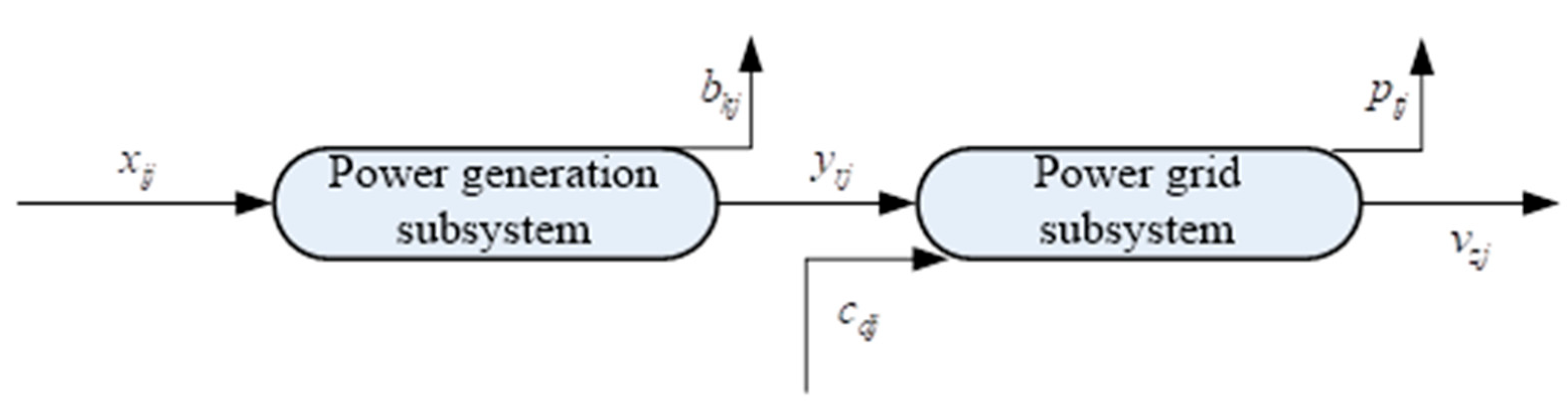
Figure 1 shows the general internal structure of the PSCS. In the power generation subsystem (PG), the inputs are ; the desirable outputs are ; and the undesirable outputs are . In the power grid subsystem (PGS), the inputs include and ; the desirable outputs are ; and the undesirable outputs are . The explanations of notations and variables are shown in Table 1.
Traditional DEA models have mostly applied the Shephard distance function [37] to evaluate the efficiency of the evaluated unit. The Shephard distance function maximizes the desirable output, but also increases the undesirable output [38]. This does not align with the practice of reducing emissions. To address this problem, Chambers et al. [39] proposed the direction distance function (DDF). The DDF method increases desirable outputs while simultaneously reducing inputs and undesirable output [40,41]. For , the production technology set is expressed as follows:
To increase the potential improvement capacity of inputs and outputs, Färe and Grosskopf [42] proposed a radial DDF approach, as follows:
In model (2), is the direction vector, representing the adjustment direction of the inputs, the undesired outputs, and the desired outputs. The variable represents the potential improvement in the PG performance, and the variable represents the potential improvement in the PGS performance. If and , the evaluated PSCS is efficient and cannot be further improved.
Regarding the treatment of weak disposability, Kuosmanen [36] observed differences in the disposability across decision-making units (DMUs); however, the traditional weak disposability method implicitly assumed that all DMUs used uniform abatement factors. Based on traditional DDF, this study further introduced Kuosmanen’s technique [36]. The possible production set of the PSCS is as follows:
Equation (3) is nonlinear and is difficult to solve. Equation (3) is made linear using the following transformation. For , we set , as representing the weights of the active outputs; and () represents the weights of the inactive outputs. For , we set , () as representing the weights of the active outputs; and () represents the weights of the inactive outputs. Hence, Equation (3) is transformed into the following linear Equation (4).
3.2. The Two-Stage Network Model
DDF models can be divided into radial and non-radial categories. The radial DDF model has two main problems. First, the radial efficiency measurement does not measure efficiencies or make recommendations for improvement for each index [43]. Second, the radial DDF model has non-zero slack variables in the evaluation process, causing it to overestimate efficiency [44]. Given these problems with the radial DDF model, this study applied non-radial DDF to construct an efficiency evaluation model for PSCS.
Based on the studies of Sun et al. [6,8], the PSCSs were divided into G groups, with the PSCSs in each group assumed to have the same or similar technical level. In the group, the group efficiency (GE) of was obtained using model (5).
In model (3), the variables represent the weights; the variable represents the number of PSs in the group; the variable represents the efficiency of ; and the variables ,, , and represent the improvement potentials of , , , and , respectively. is considered an intermediate variable connecting the two subsystems; as such, this study considered it to be a free variable. In other words, the variable can freely adjust its target based on the actual situation. Model (5) is a nonlinear model, which was converted into a linear model using the following three steps.
- Step 1:
- Let . Model (5) was transformed into model (6).
After substituting into model (5), a constraint is added to model (5). Thus model (5) is equivalent to model (6). However, the objective function of model (6) contains the multiplication of two variables, which is still non-linear and requires further conversion.
- Step 2:
- Let . By substituting these equations into model (6), model (6) was transformed into model (7).
Model (7) is linear and can be solved directly. Then, through step 3, the optimal solution of model (5) is obtained.
- Step 3:
- The optimal solutions were generated by solving model (7). Then, the optimal solutions of model (5) were obtained as follows: .
Model (7) generates the efficiency of in the group by referring to the group frontier. If is compared with all PSCSs, it may yield a different efficiency, referred to as the meta-frontier efficiency (ME) in this study. Based on the meta-frontier, the ME of was obtained using model (8):
Model (8) is a nonlinear model, which was converted into linear model (9) using the three steps described above.
The constraints of Models (5) and (9) differ; the number of PSCSs in the two models satisfies . This leads the two models to have different frontiers. Specifically, the frontier of Model (5) was formed by the optimal performing PSCSs in the group; in contrast, the frontier of Model (8) was formed by all the optimally performing PSCSs. Therefore, the Model (5) frontier represented the best technology level of the group, and the Model (8) frontier represented the best technology level of all PSCSs.
To provide targeted improvement paths for inefficient PSCSs, this study deconstructed the improvement potential of the PSCSs into management potential (MP) and technical potential (TP).
Definition 1.
For, the MP is .
The PSCSs in the group have the same or similar production technology level. Therefore, inadequate management leads to an inefficient . The distance from to the group-frontier is defined as the management potential.
Definition 2.
For, its TP is.
The group-frontier and meta-frontier represent different technology levels. After improving management capabilities, reaches the group-frontier. For to reach the meta-frontier, improvements are needed at the technical level. Therefore, the distance between the two frontiers is defined as the technical potential.
4. Empirical Analysis
4.1. Data
In 2015, the State Council of China issued “Several Opinions on Further Deepening the Reform of the Electric Power System”. The opinions proposed a series of requirements for China’s PSCS. For example, China will deepen the reform of the power system, focusing on the power generation, transmission, distribution, and sales links of the power industry chain. Specifically, power electricity is produced by the power plant, and then transmitted and distributed through the grid company, to finally reach consumers. Some studies on the environmental efficiency of PSCSs take the power system as a whole [45,46]. According to the role played by power plants and the grid company in PSCSs, this study divided the regional PSCSs into two subsystems: PG and PGS.
The inputs and outputs of PG are as follows.
Input 1: The new production capacity of the power supply construction (10,000 kilowatts) represents the newly added capacity of the power plant to put into power production in a specific period, reflecting the power supply capacity. Sun et al. [6] and Sun et al. [47] used this indicator as one of the inputs to evaluate the performance of China’s power supply chain system.
Input 2: The power generation equipment capacity at 6000 kilowatts and above (10,000 kilowatts) represents the maximum production capacity of power generation equipment. Generally, the greater the capacity, the greater the power generation capacity. Park and Lesourd [48] used this indicator as one of the inputs to evaluate the efficiency of Korean power plants. Sun et al. [49] used this indicator as one of the inputs to evaluate the efficiency of thermal power plants in China.
Input 3: The utilization hours of power generation equipment (hours) represent the average full-load operating time of power generation equipment in one year. To evaluate the sustainable performance of the power system, Sun et al. [8] used this indicator as one of the inputs.
Input 4: The coal consumption rate to generate power (g/kWh) represents the amount of coal consumed by the power plant to produce 1 kilowatt-hour of electricity, and is an indicator that reflects the energy utilization rate of power generation enterprises [50,51].
Output: The electricity generation (100 million kWh) represents the actual electric energy produced by the power plant in a certain period, which is the desired output of the power plant [52,53,54].
Undesired output: Carbon dioxide emissions (10,000 tons) represent the undesirable emissions produced by burning coal during the power generation process of a power plant and are an indicator of the environmental efficiency of the power plant [51,52,53].
The inputs and outputs of PGS are as follows.
Input 1: The newly increased capacity of 220 kV and above of the transformer equipment (ten thousand kVA) represents the increased capacity of power transformation equipment in a specific period, reflecting the power supply guarantee ability of the power grid [55].
Input 2: The length of newly added transmission lines of 220 kV and above (km) represents the length of transmission lines increased in a specific period, reflecting the power transmission capacity of the power grid [55,56].
Output: The electricity sales output value (100 million yuan) represents the electricity sales income of the power grid company, reflecting the profitability of that power grid company [56,57].
Undesired output: The line loss rate represents the percentage of power lost during transmission. It reflects the performance level of power transmission of the power grid company. The higher the line loss rate, the worse the power transmission performance of the power grid company [55,58].
In the two systems, power generation was the intermediate output. In other words, it is the desired output of PG, and it is also the input of PGS. Carbon dioxide was calculated based on raw coal consumption, and the electricity sales output value was obtained by multiplying the average sales price and electricity sales. All data are from the wind database.
To classify China’s regions, scholars have proposed different classification standards (e.g., [30,59,60]). This study explored the impact of the disposable income of residents on PSCS performance. Therefore, this study divided Chinese provinces into five regions based on the average disposable income of residents. The five areas included the low-income area, the lower-middle-income area, the middle-income area, the upper-middle-income area, and the high-income area. Table 2 shows the specific regional divisions.
4.2. Performance Analysis
Models (5) and (8) were used to generate the GE and ME of the PSCSs of different Chinese provinces from 2014 to 2017, as shown in Table 3.
Table 3 shows the following. The ME of some regions differed significantly over the four years in the study period. For example, the ME of Beijing’s PSCS experienced an increasing trend, while the ME of Hebei’s PSCS experienced a decreasing trend. These values may have been affected by local policies and measures. For example, to reduce greenhouse gas emissions, the Beijing government promulgated the “Administrative Measures on Beijing’s Carbon Emission Trading” in 2014. Implementing these “Administrative Measures” effectively reduced pollutant emissions in the power industry, advancing the efficiency of Beijing’s power system. To develop the economy, Hebei has accepted the transfer of specific industries from Beijing, including enterprises with high pollution and energy consumption. This has exacerbated the burden on Hebei’s PSCS, decreasing the efficiency of its power system.
The average ME in all regions is 0.3788. The provinces with higher average MEs included Beijing, Guangdong, Jiangsu, Zhejiang, Guangxi, Yunnan, and Qinghai. The average ME in other regions was less than 0.4. Shanxi had the lowest average ME, at only 0.1441. These results indicate that the efficiency of China’s PSCSs was generally low overall. In addition, highly efficient regions were from China’s most developed areas or the least developed economic areas.
Table 4 shows the average GE of the five areas. The average GE of the PSCSs in the middle-income area was the highest during the study period. In contrast, the average GE of the PSCSs in the upper-middle-income area was the lowest. The frontier of the group represents the best technical level of this group; the key contributor to group inefficiency was insufficient management. Therefore, the PSCSs in the upper-middle-income area appear to have the greatest management improvement potential.
Table 5 shows the average ME results of the five areas. It indicates that the average ME of the PSCSs in the middle-income area was the lowest during the study period. In contrast, the average ME of the PSCSs of the high-income area was the highest. This result is similar to the environmental Kuznets curve. This finding is consistent with the conclusion of Wang [34], who analyzed the energy conservation and emission reduction performance of 209 cities in China and found that the relationship between energy conservation and emission reduction performance and income is U-shaped. Specifically, in low-income areas (such as the low-income area and the lower-middle-income area), the level of economic development was low, with slow industrial development. Therefore, this area consumed less industrial power and had lower pollutant emissions from the PSCSs, resulting in a high ME from the PSCS. To develop the economy, middle-income areas have vigorously pursued industrial development. This has led to high power consumption, and high greenhouse gas emissions from the PSCS. This has, in turn, led to inefficient PSCSs in this area. In economically developed regions (such as the high-income area), the rapid economic development has increased the power demand in these areas [8,50], and has also promoted the investment in PCSCs in these areas. This promotes the promotion and application of power generation technology and low-carbon technology in these regions [50]. For example, Jiangsu Province established a real-time online monitoring and evaluation system for carbon emissions of thermal power companies in 2019, which effectively controls carbon emissions. As such, the efficiency of the PSCSs of this area was high.
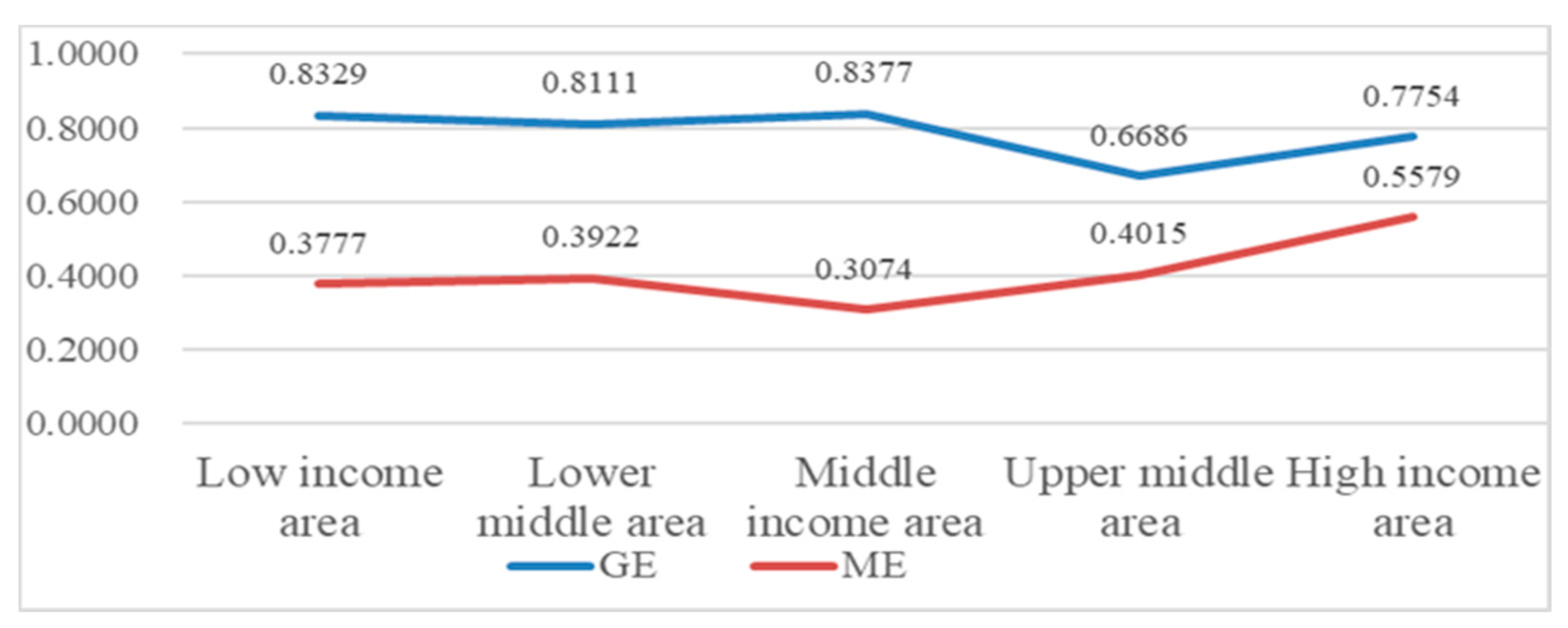
4.3. Comparison of GE and ME
Figure 2 shows the average ME and average GE of PSCSs in each area. It demonstrates that the average ME of each area did not exceed its GE in the study period. The gap between the GE and ME in the high-income area was the smallest. In contrast, there was a large gap between the GE and ME in the middle-income area. There are two main reasons for this result. First, the provinces in the high-income area are located in China’s economically developed regions. Economic development has led these provinces to invest more in the PSCS, resulting in a higher technology level in the PSCS. Second, the provinces in the middle-income area are located in the northeast and central regions of China, which are rich in coal resources. The unreasonable industrial structure in these areas has caused economic development to be restricted. In addition, abundant coal resources mean that these areas lack the capacity to upgrade power generation technology and equipment. The coal-fired power generation enterprises have low resource utilization and emit large amounts of carbon dioxide. These factors led to the low efficiency of the PSCSs in these areas.
4.4. Performance Improvement Path
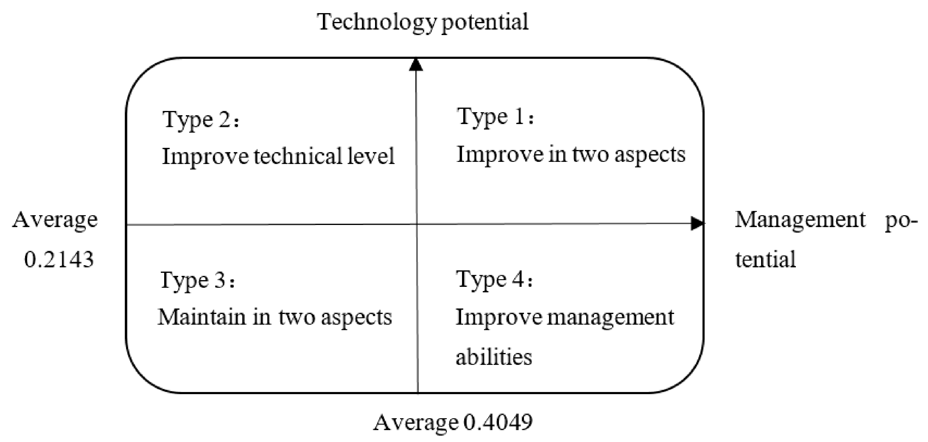
To propose improvements for regions with inefficient PSCS performance, the MP and TP of each PSCS were calculated and analyzed to identify performance improvement targets. Figure 3 and Table 6 show the specific results.
The regions of Type 1 include the provincial PSCSs in Shaanxi and Heilongjiang. They showed deficiencies in both management and technology, and their MP and TP were higher than the national average. These PSCSs should implement effective measures in both management and technology to improve their efficiency. This could include updating equipment, learning advanced management methods, and learning from other regions’ experiences.
The regions of Type 2 contain 13 provincial PSCSs. The management capacity of these PSCSs was higher than the national average, but the technology was insufficient. To improve PSCS performance, these regions should increase their investment in technology and introduce advanced technology to improve their technical level.
The regions of Type 3 include the PSCSs in Qinghai and Guangdong. The management capacity and technical level of these PSCSs were higher than the national average. Therefore, the PSCSs in these two areas should maintain their current advantages.
The regions of Type 4 include 8 provincial PSCSs. The management capacity of these PSCSs was lower than the national average. To reduce the efficiency loss caused by insufficient management, these PSCSs should make long-term efforts to improve management capabilities, such as learning from the excellent management approaches used by the third category of PSCSs, formulating power policies, and strengthening power system oversight.
5. Conclusions
The power industry has made significant contributions to China’s economic development and industrialized production. However, thermal power generation comprises a large proportion of power production in China, with high energy consumption and emissions. In addition, there is a high line loss rate from the power grid. To analyze the performance of China’s regional PSCSs, this study proposed two non-radial DEA models. The developed proposed models effectively measured PSCS performance in different regions of China, and deconstructed the sources of inefficiency into management potential and technology potential. The study’s empirical analysis further analyzed the impact of residents’ disposable income on PSCS performance.
Through the calculation of the models, the empirical analysis of this study generated the following key research findings. First, based on model (5) and model (8), the efficiency values of PSCSs of 24 regions from 2014 to 2017 were obtained, as shown in Table 3. This study found that China had a low overall PSCS performance (0.3788), with significant potential for improvement. Second, Table 3 also shows that PSCS performance varied significantly over time in different regions. Third, the results in Table 6, calculated by model (8), show that the PSCSs in high-income regions had the highest average ME, while the PSCSs in middle-income regions had the lowest average ME. This result is consistent with the environmental Kuznets curve hypothesis. Fourth, based on the definitions of MP and TP, the MP and TP of each region were calculated. The results are shown in Table 6. The results in Table 6 show that the management and technical levels of PSCSs in Qinghai and Guangdong performed well. The PSCSs in other regions need to address management inadequacies, technical insufficiencies, or both.
These findings highlight three key policy recommendations for China’s PSCSs. The first policy recommendation is to determine the optimal benchmark PSCS for inefficient PSCSs in the same group. For example, the results in Table 3 show that in the high-income group, the PSCSs in Jiangsu and Zhejiang can be used as the benchmark for other PSCSs in the same group. Inefficient PSCSs can refer to the experience of PSCSs in Jiangsu and Zhejiang to improve performance. Similarly, in other groups, PSCSs in Liaoning, Jiangxi, Guangxi, and Guizhou can be used as the optimal benchmarks.
The second recommendation is to improve the economic development model of middle-income regions. Compared with other groups, the meta-frontier efficiency of PSCSs in the middle-income group is lower. The PSCSs of the middle-income group mainly come from the northeast and central regions of China. These areas are currently actively introducing heavy industrial industries, which makes the demand for electricity huge. Unsustainable economic development has led to high carbon emissions and low energy efficiency. Therefore, the PSCSs in these areas are inefficient. The PSCSs of the middle-income group need to implement a high-quality economic development mode and adhere to the coordinated development of the economy and the ecological environment. This is an effective way for the PSCSs of the middle-income area to improve efficiency.
The third policy recommendation is to determine approaches by which a PSCS can improve its efficiency in a targeted manner. This study broke down the performance improvement potential of PSCSs into MP and TP. The economic development level, scale and energy resources are different across China’s regions, and each region should clarify the direction of its performance improvement based on the actual situation. This study divided the PSCSs of different provinces in China into four types, and proposed specific efficiency improvement strategies for each PSCS type. For example, for the first type of PSCS, technical deficiencies cannot be eliminated in the short term. As such, inefficient PSCSs should focus on improving short-term management capabilities, such as improving education on excellent management practices and formulating policies. Once the short-term goal is achieved, the inefficient PSCSs should improve their technical level by updating production equipment and introducing technology and technological innovations. In addition, there is a significant positive correlation between the scale and efficiency of the power system [17]. The larger the scale, the higher the efficiency. Therefore, the scale of the first type of PSCS can be appropriately expanded to further improve its environmental efficiency.
Author Contributions
Conceptualization, D.H.; methodology, F.H.; software, Y.D.; data curation, Y.D.; writing—original draft preparation, F.H., Y.D.; formal analysis, B.Z.; supervision, D.H. All authors have read and agreed to the published version of the manuscript.
Funding
This research was supported by the National Natural Science Foundation of China (Project no. 71871153) and National Social Science Foundation of China (Project no. 19BGL188).
Institutional Review Board Statement
Not applicable.
Informed Consent Statement
Not applicable.
Data Availability Statement
Not applicable.
Conflicts of Interest
The authors declare no conflict of interest.
References
- Zhou, Y.; Xing, X.; Fang, K.; Liang, D.; Xu, C. Environmental efficiency analysis of power industry in China based on an entropy SBM model. Energy Policy 2013, 57, 68–75. [Google Scholar] [CrossRef]
- Sergi, B.; Azevedo, I.; Xia, T.; Davis, A.; Xu, J. Support for emissions reductions based on immediate and long-term pollution exposure in China. Ecol. Econ. 2019, 158, 26–33. [Google Scholar] [CrossRef]
- Kopas, J.; York, E.; Jin, X.; Harish, S.; Kennedy, R.; Shen, S.V.; Urpelainen, J. Environmental justice in India: Incidence of air pollution from coal-fired power plants. Ecol. Econ. 2020, 176, 106711. [Google Scholar] [CrossRef]
- Jiang, P.; Khishgee, S.; Alimujiang, A.; Dong, H. Cost-effective approaches for reducing carbon and air pollution emissions in the power industry in China. J. Environ. Manag. 2020, 264, 110452. [Google Scholar] [CrossRef] [PubMed]
- Tang, B.-J.; Li, R.; Li, X.-Y.; Chen, H. An optimal production planning model of coal-fired power industry in China: Considering the process of closing down inefficient units and developing CCS technologies. Appl. Energy 2017, 206, 519–530. [Google Scholar] [CrossRef]
- Sun, J.; Xu, S.; Li, G. Analyzing sustainable power supply chain performance. J. Enterp. Inf. Manag. 2020, 34, 79–100. [Google Scholar] [CrossRef]
- Yao, X.; Huang, R.; Du, K. The impacts of market power on power grid efficiency: Evidence from China. China Econ. Rev. 2019, 55, 99–110. [Google Scholar] [CrossRef]
- Sun, J.; Li, G.; Lim, M.K. China’s power supply chain sustainability: An analysis of performance and technology gap. Ann. Oper. Res. 2020. [Google Scholar] [CrossRef]
- Wu, J.; Lv, L.; Sun, J.; Ji, X. A comprehensive analysis of China’s regional energy saving and emission reduction efficiency: From production and treatment perspectives. Energy Policy 2015, 84, 166–176. [Google Scholar] [CrossRef]
- Wu, J.; Sun, J.; Liang, L. Methods and applications of DEA cross-efficiency: Review and future perspectives. Front. Eng. Manag. 2021, 8, 199–211. [Google Scholar] [CrossRef]
- Färe, R.; Grosskopf, S.; Logan, J. The relative performance of publicly-owned and privately-owned electric utilities. J. Public Econ. 1985, 26, 89–106. [Google Scholar] [CrossRef]
- Golany, B.; Roll, Y.; Rybak, D. Measuring efficiency of power plants in Israel by data envelopment analysis. IEEE Trans. Eng. Manag. 1994, 41, 291–301. [Google Scholar] [CrossRef]
- Sueyoshi, T.; Goto, M. Slack-adjusted DEA for time series analysis: Performance measurement of Japanese electric power generation industry in 1984–1993. Eur. J. Oper. Res. 2001, 133, 232–259. [Google Scholar] [CrossRef]
- Arocena, P. Cost and quality gains from diversification and vertical integration in the electricity industry: A DEA approach. Energy Econ. 2008, 30, 39–58. [Google Scholar] [CrossRef]
- Sueyoshi, T.; Goto, M. Efficiency-based rank assessment for electric power industry: A combined use of Data Envelopment Analysis (DEA) and DEA-Discriminant Analysis (DA). Energy Econ. 2012, 34, 634–644. [Google Scholar] [CrossRef]
- Xin-Gang, Z.; Zhen, W. The technical efficiency of China’s wind power list enterprises: An estimation based on DEA method and micro-data. Renew. Energy 2019, 133, 470–479. [Google Scholar] [CrossRef]
- Zhang, N.; Kong, F.; Choi, Y.; Zhou, P. The effect of size-control policy on unified energy and carbon efficiency for Chinese fossil fuel power plants. Energy Policy 2014, 70, 193–200. [Google Scholar] [CrossRef]
- Chen, W.; Zhou, K.; Yang, S. Evaluation of China’s electric energy efficiency under environmental constraints: A DEA cross efficiency model based on game relationship. J. Clean. Prod. 2017, 164, 38–44. [Google Scholar] [CrossRef]
- Wang, K.; Zhang, J.; Wei, Y.-M. Operational and environmental performance in China’s thermal power industry: Taking an effectiveness measure as complement to an efficiency measure. J. Environ. Manag. 2017, 192, 254–270. [Google Scholar] [CrossRef]
- Sartori, S.; Witjes, S.; Campos, L.M. Sustainability performance for Brazilian electricity power industry: An assessment integrating social, economic and environmental issues. Energy Policy 2017, 111, 41–51. [Google Scholar] [CrossRef] [Green Version]
- Chen, Z.; Li, J.; Zhao, W.; Yuan, X.-C.; Yang, G.-L. Undesirable and desirable energy congestion measurements for regional coal-fired power generation industry in China. Energy Policy 2019, 125, 122–134. [Google Scholar] [CrossRef]
- Cooper, W.; Deng, H.; Gu, B.; Li, S.; Thrall, R. Using DEA to improve the management of congestion in Chinese industries (1981–1997). Socio Econ. Plan. Sci. 2001, 35, 227–242. [Google Scholar] [CrossRef]
- Zhou, D.; Meng, F.; Bai, Y.; Cai, S. Energy efficiency and congestion assessment with energy mix effect: The case of APEC countries. J. Clean. Prod. 2017, 142, 819–828. [Google Scholar] [CrossRef]
- Seiford, L.M.; Zhu, J. Profitability and marketability of the top 55 U.S. commercial banks. Manag. Sci. 1999, 45, 1270–1288. [Google Scholar] [CrossRef] [Green Version]
- Kao, C.; Hwang, S.-N. Efficiency decomposition in two-stage data envelopment analysis: An application to non-life insurance companies in Taiwan. Eur. J. Oper. Res. 2008, 185, 418–429. [Google Scholar] [CrossRef]
- Chen, Y.; Cook, W.D.; Li, N.; Zhu, J. Additive efficiency decomposition in two-stage DEA. Eur. J. Oper. Res. 2009, 196, 1170–1176. [Google Scholar] [CrossRef]
- Wang, Q.; Wu, Z.; Chen, X. Decomposition weights and overall efficiency in a two-stage DEA model with shared resources. Comput. Ind. Eng. 2019, 136, 135–148. [Google Scholar] [CrossRef]
- Zhu, W.; Zhang, Q.; Wang, H. Fixed costs and shared resources allocation in two-stage network DEA. Ann. Oper. Res. 2017, 278, 177–194. [Google Scholar] [CrossRef]
- Chu, J.; Wu, J.; Chu, C.; Zhang, T. DEA-based fixed cost allocation in two-stage systems: Leader-follower and satisfaction degree bargaining game approaches. Omega 2020, 94, 102054. [Google Scholar] [CrossRef]
- Sun, J.; Li, G.; Wang, Z. Technology heterogeneity and efficiency of China’s circular economic systems: A game meta-frontier DEA approach. Resour. Conserv. Recycl. 2019, 146, 337–347. [Google Scholar] [CrossRef]
- Yin, P.; Chu, J.; Wu, J.; Ding, J.; Yang, M.; Wang, Y. A DEA-based two-stage network approach for hotel performance analysis: An internal cooperation perspective. Omega 2020, 93, 102035. [Google Scholar] [CrossRef]
- Taskin, F.; Zaim, O. The role of international trade on environmental efficiency: A DEA approach. Econ. Model. 2001, 18, 1–17. [Google Scholar] [CrossRef]
- Halkos, G.E.; Tzeremes, N.G. Exploring the existence of Kuznets curve in countries’ environmental efficiency using DEA window analysis. Ecol. Econ. 2009, 68, 2168–2176. [Google Scholar] [CrossRef]
- Wang, Q.; Su, B.; Sun, J.; Zhou, P.; Zhou, D. Measurement and decomposition of energy-saving and emissions reduction performance in Chinese cities. Appl. Energy 2015, 151, 85–92. [Google Scholar] [CrossRef]
- Halkos, G.E.; Polemis, M.L. The impact of economic growth on environmental efficiency of the electricity sector: A hybrid window DEA methodology for the USA. J. Environ. Manag. 2018, 211, 334–346. [Google Scholar] [CrossRef]
- Kuosmanen, T. Weak disposability in nonparametric production analysis with undesirable outputs. Am. J. Agric. Econ. 2005, 87, 1077–1082. [Google Scholar] [CrossRef]
- Pyatt, G.; Shephard, R.W. Theory of cost and production functions. Econ. J. 1972, 82, 1059. [Google Scholar] [CrossRef]
- Chung, Y.; Färe, R.; Grosskopf, S. Productivity and undesirable outputs: A directional distance function approach. J. Environ. Manag. 1997, 51, 229–240. [Google Scholar] [CrossRef] [Green Version]
- Chambers, R.G.; Chung, Y.; Färe, R. Benefit and distance functions. J. Econ. Theory 1996, 70, 407–419. [Google Scholar] [CrossRef]
- Picazo-Tadeo, A.J.; Castillo-Giménez, J.; Beltrán-Esteve, M. An intertemporal approach to measuring environmental performance with directional distance functions: Greenhouse gas emissions in the European Union. Ecol. Econ. 2014, 100, 173–182. [Google Scholar] [CrossRef]
- Li, H.-L.; Zhu, X.-H.; Chen, J.-Y.; Jiang, F.-T. Environmental regulations, environmental governance efficiency and the green transformation of China’s iron and steel enterprises. Ecol. Econ. 2019, 165, 106397. [Google Scholar] [CrossRef]
- Färe, R.; Grosskopf, S. Directional distance functions and slacks-based measures of efficiency. Eur. J. Oper. Res. 2010, 206, 702. [Google Scholar] [CrossRef]
- Chang, T.-P.; Hu, J.-L. Total-factor energy productivity growth, technical progress, and efficiency change: An empirical study of China. Appl. Energy 2010, 87, 3262–3270. [Google Scholar] [CrossRef]
- Fukuyama, H.; Weber, W.L. A directional slacks-based measure of technical inefficiency. Socio Econ. Plan. Sci. 2009, 43, 274–287. [Google Scholar] [CrossRef]
- Wang, K.; Wei, Y.-M.; Huang, Z. Environmental efficiency and abatement efficiency measurements of China’s thermal power industry: A data envelopment analysis based materials balance approach. Eur. J. Oper. Res. 2018, 269, 35–50. [Google Scholar] [CrossRef]
- Yu, X.; Jin, L.; Wang, Q.; Zhou, D. Optimal path for controlling pollution emissions in the Chinese electric power industry considering technological heterogeneity. Environ. Sci. Pollut. Res. 2019, 26, 11087–11099. [Google Scholar] [CrossRef]
- Sun, J.; Xu, S.; Li, G. Does China’s power supply chain systems perform well? A data-based path-index meta-frontier analysis. Ind. Manag. Data Syst. 2020. [Google Scholar] [CrossRef]
- Park, S.-U.; LeSourd, J.-B. The efficiency of conventional fuel power plants in South Korea: A comparison of parametric and non-parametric approaches. Int. J. Prod. Econ. 2000, 63, 59–67. [Google Scholar] [CrossRef]
- Sun, C.; Liu, X.; Li, A. Measuring unified efficiency of Chinese fossil fuel power plants: Intermediate approach combined with group heterogeneity and window analysis. Energy Policy 2018, 123, 8–18. [Google Scholar] [CrossRef]
- Eguchi, S.; Takayabu, H.; Lin, C. Sources of inefficient power generation by coal-fired thermal power plants in China: A metafrontier DEA decomposition approach. Renew. Sustain. Energy Rev. 2021, 138, 110562. [Google Scholar] [CrossRef]
- Li, L. Carbon emission reduction of power enterprises in subtropical and temperate regions of China. Trop. Conserv. Sci. 2019, 12. [Google Scholar] [CrossRef]
- Long, X.; Wu, C.; Zhang, J.; Zhang, J. Environmental efficiency for 192 thermal power plants in the Yangtze River delta considering heterogeneity: A metafrontier directional slacks-based measure approach. Renew. Sustain. Energy Rev. 2018, 82, 3962–3971. [Google Scholar] [CrossRef]
- Wu, C.; Oh, K.; Long, X.; Zhang, J. Effect of installed capacity size on environmental efficiency across 528 thermal power stations in North China. Environ. Sci. Pollut. Res. 2019, 26, 29822–29833. [Google Scholar] [CrossRef]
- Wang, C.; Cao, X.; Mao, J.; Qin, P. The changes in coal intensity of electricity generation in Chinese coal-fired power plants. Energy Econ. 2019, 80, 491–501. [Google Scholar] [CrossRef]
- Zhao, H.; Zhao, H.; Guo, S. Operational efficiency of Chinese provincial electricity grid enterprises: An evaluation employing a three-stage data envelopment analysis (DEA) Model. Sustainability 2018, 10, 3168. [Google Scholar] [CrossRef] [Green Version]
- Tang, H.; Yu, S. Evaluation of operational efficiency of power grid enterprises based on DEA. Technoecon. Manag. Res. 2012, 4, 8–11. (In Chinese) [Google Scholar] [CrossRef]
- Tone, K.; Tsutsui, M. Network DEA: A slacks-based measure approach. Eur. J. Oper. Res. 2009, 197, 243–252. [Google Scholar] [CrossRef] [Green Version]
- Liu, Y.; Wang, M.; Liu, X.; Xiang, Y. Evaluating investment strategies for distribution networks based on yardstick competition and DEA. Electr. Power Syst. Res. 2019, 174, 105868. [Google Scholar] [CrossRef]
- Liu, X.; Wu, J. Energy and environmental efficiency analysis of China’s regional transportation sectors: A slack-based DEA approach. Energy Syst. 2015, 8, 747–759. [Google Scholar] [CrossRef]
- Sun, J.; Li, G.; Wang, Z. Optimizing China’s energy consumption structure under energy and carbon constraints. Struct. Chang. Econ. Dyn. 2018, 47, 57–72. [Google Scholar] [CrossRef]
Figure 1.
The internal structure of the power supply chain system.

Figure 2.
The average GE and ME of each area.

Figure 3.
The sources of performance improvement.


Table 1.
Summary of notations and variables.
| Notation/Variable | Explanation |
|---|---|
| The ith input of | |
| The kth undesirable output of | |
| The rth desirable output of | |
| The dth input of | |
| The zth output of | |
| The tth undesirable output of | |
| The weights of | |
| The weights of | |
| Emission reduction factor | |
| The weights of under the group-frontier | |
| The weights of under the meta-frontier | |
| The weights of under the group-frontier | |
| The weights of under the meta-frontier | |
| Reduction potential of inputs in | |
| Reduction potential of undesired outputs of | |
| Reduction potential of inputs in | |
| Reduction potential of undesired outputs in | |
| Increased potential of desired outputs in |
Table 2.
Regional divisions.
| Areas | Provinces |
|---|---|
| Low-income area | Gansu, Guizhou, Yunnan, Qinghai |
| Lower-middle-income area | Guangxi, Henan, Sichuan, Shaanxi, Shanxi |
| Middle-income area | Hebei, Anhui, Heilongjiang, Jiangxi, Jilin, Hunan |
| Upper-middle-income area | Hubei, Inner Mongolia, Shandong, Liaoning, Guangdong |
| High-income area | Jiangsu, Tianjin, Zhejiang, Beijing |
Table 3.
Efficiency of power supply chain systems of all provinces from 2014 to 2017.
| Region | GE | ME | ||||||||
|---|---|---|---|---|---|---|---|---|---|---|
| 2014 | 2015 | 2016 | 2017 | Average | 2014 | 2015 | 2016 | 2017 | Average | |
| Beijing | 0.4910 | 0.7599 | 0.7187 | 1.0000 | 0.7424 | 0.4839 | 0.7596 | 0.7124 | 1.0000 | 0.7390 |
| Tianjin | 0.3478 | 0.4761 | 0.2831 | 0.4751 | 0.3955 | 0.3357 | 0.4460 | 0.2608 | 0.4476 | 0.3725 |
| Jiangsu | 1.0000 | 0.9388 | 1.0000 | 1.0000 | 0.9847 | 0.5491 | 0.5488 | 0.5593 | 0.6051 | 0.5656 |
| Zhejiang | 0.9522 | 0.9630 | 1.0000 | 1.0000 | 0.9788 | 0.5440 | 0.5393 | 0.5930 | 0.5425 | 0.5547 |
| Hebei | 1.0000 | 0.8346 | 0.7809 | 0.8116 | 0.8568 | 0.5757 | 0.3226 | 0.2877 | 0.2921 | 0.3695 |
| Shandong | 0.4292 | 0.3872 | 0.3046 | 0.3219 | 0.3607 | 0.3497 | 0.3416 | 0.2956 | 0.3096 | 0.3241 |
| Guangdong | 0.9085 | 0.9141 | 1.0000 | 1.0000 | 0.9557 | 0.8585 | 0.8800 | 0.8965 | 1.0000 | 0.9088 |
| Liaoning | 1.0000 | 1.0000 | 0.8559 | 1.0000 | 0.9640 | 0.3115 | 0.3110 | 0.2914 | 0.4076 | 0.3304 |
| Jilin | 0.7847 | 1.0000 | 0.7199 | 1.0000 | 0.8762 | 0.2689 | 0.2912 | 0.2446 | 0.5378 | 0.3357 |
| Heilongjiang | 0.8750 | 0.7499 | 0.6428 | 0.6741 | 0.7355 | 0.2413 | 0.2824 | 0.2315 | 0.2424 | 0.2494 |
| Shanxi | 0.5615 | 0.5126 | 0.4951 | 0.5476 | 0.5292 | 0.1606 | 0.1454 | 0.1338 | 0.1365 | 0.1441 |
| Anhui | 0.5866 | 0.6124 | 0.5523 | 0.7084 | 0.6149 | 0.2257 | 0.2145 | 0.1947 | 0.2216 | 0.2141 |
| Jiangxi | 1.0000 | 1.0000 | 0.9013 | 1.0000 | 0.9753 | 0.4191 | 0.2997 | 0.2811 | 0.3178 | 0.3294 |
| Henan | 1.0000 | 1.0000 | 1.0000 | 1.0000 | 1.0000 | 0.4200 | 0.2888 | 0.2918 | 0.2736 | 0.3186 |
| Hubei | 1.0000 | 1.0000 | 0.9887 | 0.4856 | 0.8686 | 0.3426 | 0.3409 | 0.2662 | 0.2706 | 0.3051 |
| Hunan | 1.0000 | 0.8935 | 1.0000 | 0.9780 | 0.9679 | 0.4215 | 0.3096 | 0.3225 | 0.3318 | 0.3464 |
| Inner Mongolia | 0.1457 | 0.2252 | 0.1253 | 0.2797 | 0.1940 | 0.1378 | 0.1431 | 0.1159 | 0.1605 | 0.1393 |
| Guangxi | 1.0000 | 1.0000 | 0.9363 | 1.0000 | 0.9841 | 0.3831 | 0.4079 | 0.7502 | 0.3954 | 0.4841 |
| Sichuan | 0.7492 | 0.7673 | 1.0000 | 1.0000 | 0.8791 | 0.1815 | 0.2252 | 0.3589 | 0.2363 | 0.2505 |
| Guizhou | 1.0000 | 1.0000 | 0.8106 | 1.0000 | 0.9526 | 0.2889 | 0.3050 | 0.2492 | 0.3022 | 0.2863 |
| Yunnan | 1.0000 | 0.9137 | 0.8458 | 1.0000 | 0.9399 | 0.2572 | 0.2825 | 0.4672 | 1.0000 | 0.5017 |
| Shaanxi | 0.6629 | 0.5069 | 0.5840 | 0.8978 | 0.6629 | 0.3294 | 0.1938 | 0.2394 | 0.1983 | 0.2402 |
| Gansu | 0.4456 | 0.3882 | 0.7279 | 0.4935 | 0.5138 | 0.1418 | 0.1390 | 0.3039 | 0.1605 | 0.1863 |
| Qinghai | 1.0000 | 1.0000 | 1.0000 | 0.7015 | 0.9254 | 0.4272 | 0.4031 | 1.0000 | 0.3149 | 0.5363 |
Table 4.
Statistical description of GE.
| Areas | Max | Min | Median | Mean | Std. |
|---|---|---|---|---|---|
| Low-income area | 1.0000 | 0.3882 | 0.9568 | 0.8329 | 0.2124 |
| Lower-middle income area | 1.0000 | 0.4951 | 0.9171 | 0.8111 | 0.2046 |
| Middle-income area | 1.0000 | 0.5523 | 0.8548 | 0.8377 | 0.1506 |
| Upper-middle-income area | 1.0000 | 0.1253 | 0.8822 | 0.6686 | 0.3438 |
| High-income area | 1.0000 | 0.2831 | 0.9455 | 0.7754 | 0.2604 |
Table 5.
Statistical description of ME.
| Areas | Max | Min | Median | Mean | Std. |
|---|---|---|---|---|---|
| Low-income area | 1.0000 | 0.1390 | 0.3031 | 0.3777 | 0.2517 |
| Lower-middle-income area | 1.0000 | 0.1338 | 0.2918 | 0.3922 | 0.2578 |
| Middle-income area | 0.5757 | 0.1947 | 0.2895 | 0.3074 | 0.0934 |
| Upper-middle-income area | 1.0000 | 0.1159 | 0.3112 | 0.4015 | 0.2659 |
| High-income area | 1.0000 | 0.2608 | 0.5464 | 0.5579 | 0.1643 |
Table 6.
Classification of regional PSCSs.
| Low-Income Area | Lower-Middle-Income Area | Middle-Income Area | Upper-Middle-Income Area | High-Income Area | |
|---|---|---|---|---|---|
| Type 1 | Shaanxi | Heilongjiang | |||
| Type 2 | Guizhou, Yunnan | Guangxi, Henan, Sichuan | Hebei, Jiangxi, Jilin, Hunan | Hubei, Liaoning | Jiangsu, Zhejiang |
| Type 3 | Qinghai | Guangdong | |||
| Type 4 | Gansu | Shanxi | Anhui | Inner Mongolia, Shandong | Tianjin, Beijing |
Publisher’s Note: MDPI stays neutral with regard to jurisdictional claims in published maps and institutional affiliations. |
© 2021 by the authors. Licensee MDPI, Basel, Switzerland. This article is an open access article distributed under the terms and conditions of the Creative Commons Attribution (CC BY) license (https://creativecommons.org/licenses/by/4.0/).
Share and Cite
MDPI and ACS Style
Huang, F.; Du, Y.; Hu, D.; Zhang, B. Sustainable Performance Analysis of Power Supply Chain System from the Perspective of Technology and Management. Sustainability 2021, 13, 5972. https://0-doi-org.brum.beds.ac.uk/10.3390/su13115972
AMA Style
Huang F, Du Y, Hu D, Zhang B. Sustainable Performance Analysis of Power Supply Chain System from the Perspective of Technology and Management. Sustainability. 2021; 13(11):5972. https://0-doi-org.brum.beds.ac.uk/10.3390/su13115972
Chicago/Turabian StyleHuang, Feihua, Yue Du, Debao Hu, and Bin Zhang. 2021. "Sustainable Performance Analysis of Power Supply Chain System from the Perspective of Technology and Management" Sustainability 13, no. 11: 5972. https://0-doi-org.brum.beds.ac.uk/10.3390/su13115972
Note that from the first issue of 2016, this journal uses article numbers instead of page numbers. See further details here.