Comparison of Driving Forces to Increasing Traffic Flow and Transport Emissions in Philippine Regions: A Spatial Decomposition Study

Abstract

The warming of the climate system has raised a lot of concerns for decades, and this is traceable to human activities and energy use. Conspicuously, the transportation sector is a great contributor to global emissions. This is largely due to increasing dependence on private vehicles and a poorly planned public transportation system. In addition to economic impacts, this also has significant environmental and sustainability implications. This study demonstrates a novel approach using spatial logarithmic mean Divisia index (LMDI) to analyze drivers of traffic flow and its corresponding CO₂ emissions in regions through an illustrative case study in the Philippines. Population growth is revealed as the main driver to traffic flow in most regions with the exception of a few regions and the national capital which are driven by economic activity. The economic activity effect shows positive trends contributing positively to traffic flow which is greatly linked to income level rise and increase in vehicle ownership. Concerning the impacts, results revealed that an increase in economic activity generally causes traffic intensity to decrease, and switching to more sustainable modes is not a guarantee to reduce carbon emissions. The authors recommend increasing equity on the appropriation of transport infrastructure projects across regions, quality improvement of public transport services and promoting mixed-use development.

1. Introduction

Scientific assessments disclosed by the Philippine Atmospheric, Geophysical and Astronomical Services Administration (PAGASA) revealed that the warming of the climate system is likely due to human activities such as the combustion of fossil fuels and land use [1]. Human influence on the climate system is clear, and climate change is among the most critical global issues that must be addressed. From a global report, the most important drivers of increases in CO₂ emissions from fossil fuel combustion had been traced to economic and population growth [2]. According to a report from the International Energy Agency [3], the annual CO₂ emissions from fossil fuels have increased from an estimate of 23.6 billion tons of carbon dioxide (GtCO₂) to around 32.4 GtCO₂ from 1990 to 2014, and in 2018, the global energy consumption grew almost twice the average growth rate since 2010 [4]. Coincidentally, transportation is noted to be the fastest consumer of fossil fuels and source of carbon emissions. In 2012, the transportation sector accounted for 23% of global CO₂ emissions due to fossil fuel combustion. With rapid urbanization in developing countries, energy consumption and CO₂ emissions by metropolitan vehicles are expanding quickly as the transport sector continues to experience challenges in reducing CO₂ emissions [5]. In line with this, carbon emissions from the transport sector are gradually increasing each year, responsible for approximately 24% of global carbon emissions in 2018 [6]. On the other hand, GDP growth remains to be the leading factor in energy consumption growth [7].

To further reveal transportation problems and gaps, a large body of literature has examined the drivers of increasing energy use and emissions from transport. Chen and Yang [8] further disclosed that energy-related emissions are linked to economic growth and the population’s standard of living and suggested a shift in the economic structure towards sectors with lower energy intensity. Dangay and Gately [9] carried out an investigation and projection of income’s impact on global vehicle ownership utilizing the Gompertz function and inferred that there exists a solid connection between the growth of per capita income and the growth of vehicle ownership per capita. As per capita income increases, so will the number of vehicles until saturation is reached. To address increasing vehicle use, Martin et al. [10] recommended carsharing for non-work-related travel. In support of alternatives, Ubando et al. [11] proposed an optimization methodology for electric vehicle use, considering the capital expense and power costs. Papagiannaki and Diakoulaki [12] focused on changes in transportation profiles to explain the rapid growth of the transport sector, while Jiang [13] found a surge in car ownership, with the modal share effect being consistently positive, suggesting that more people are preferring less efficient modes. In conjunction with this, Ding et al. [14] noted that the growth in transport CO₂ emissions is primarily due to modal shifts. Wang et al. [15] introduced the avoid, shift and improve approaches focusing on passenger transport. Guo et al. [16] further highlighted the need to approach each region or country exclusively to further understand the main drivers. In previous studies, multi-regional studies have been conducted through independent decomposition analyses and then comparing the different indices and major drivers among regions. While previous studies have unveiled the drivers of increasing transport activity, energy use and emissions using country- or city-specific temporal data, there exists a gap in the literature with regards to the spatial comparison of these drivers. As different cities, countries and regions can adopt different growth trajectories, they can experience different futures, may it be sustainable or unsustainable.

In response to the above-identified gaps in transport issues, researchers find index decomposition as a suitable technique to investigate transport-related problems. Index decomposition analysis is one of the techniques widely used in analyzing the change of energy consumption over a period. Plenty of related studies have used the logarithmic mean Divisia index (LMDI) method to analyze transport sector problems after it was first introduced by Ang et al. [17]. The two primarily utilized decomposition analysis techniques are the Laspeyres and Divisia related methods in Ang [18]. The LMDI technique is favored over other approaches because of its ideal decomposition and capacity to deal with cases with zero quantities. LMDI has been demonstrated to be multidisciplinary, such as in Lopez et al. [19], dissecting the impacts of various drivers to fuel combustion and electricity generation in the Philippines, and in Lopez et al. [6], which further broke down the drivers to CO₂ emissions from the Philippine transportation sector. Ang [20], in addition, provided a practical guide and case studies in decomposing industrial energy consumption and environmental emissions. Due to the gap in comparing regions, cities, or countries, Ang [21] introduced a novel methodology for using LMDI in spatial studies. This approach provides a simple but informative way to benchmark between cities, regions, or countries compared to the traditional temporal-based LMDI.

In this present work, the authors utilize a novel application of the spatial LMDI methodology by Ang [21] to road transportation. As different regions are currently on different stages and trajectories of development, each one can be taken as a representative of a particular stage. Thus, the hypothesis of this study is that data from each region can be used to predict what can happen to other regions as they adopt the same development trajectory. This approach promises interesting insights which can be used for reviewing existing sustainable transport policies and recommending new ones.

The paper proceeds as follows: Section 2 presents a literature review; Section 3 discusses the methodology and data sources for the study; Section 4 discusses the results and Section 5 concludes the study.

2. Literature Review

In this section, key drivers and findings from existing studies using decomposition analysis to address transportation issues are summarized (see

Table 1. Summary of the literature review using decomposition analysis to solve transportation problems.

Author/s	Drivers Identified	Field of Study	Method
Feng et al. [22]	Scale impact (largest); production innovation; energy-saving innovation; and energy structure.	Transport sector (China)	LMDI * (temporal) and production theoretical decomposition analysis (PDA)
Sorrell et al. [23]	Value of domestically manufactured goods to GDP.	Road freight energy use (UK)	LMDI (temporal)
Papagiannaki and Diakoulaki [12]	Passenger car usage.	Road transport CO2 emissions (Greece and Denmark)	LMDI (temporal)
Lu et al. [24]	Economic activity and vehicle ownership (contributor); population intensity (inhibitor).	Transport CO2 emissions (Germany, Japan, South Korea and Taiwan)	Divisia index decomposition analysis (DIDA)
Kwon [25]	Vehicle driving distance per individual.	Vehicle CO2 emissions (Great Britain)	Index decomposition analysis (IDA) (temporal)
Liu and Feng [26]	Per capita service output (contributor); urbanization (inhibitor).	Transport energy and CO2 emissions (China)	LMDI (temporal)
Andreoni and Galmarini [27]	Economic growth	Water and aviation transport sector (14 European Countries)	LMDI (temporal)
Timilsina and Shrestha [28]	Economic growth and transportation energy intensity.	Transport sector (20 Latin American countries)	LMDI (temporal)
Zhang, Liu and Yao [29]	Income (largest), energy intensity and transportation structure.	Transport sector (China)	LMDI (temporal and Spatial decomposition SD)
Tu et al. [30]	Mode structure and motorization	Urban transport sectors (London, Paris, New York and Tokyo)	LMDI (temporal)
Cao et al. [31]	Aviation transport	Regional transport modes CO2 emissions (Pearl River Delta)	LMDI (temporal)
Feng, Xia and Sun [32]	Transportation demand and urbanization (contributor); energy intensity and industrial structure (inhibitor).	Transport CO2 emissions (China)	LMDI (temporal)
Li et al. [33]	Income (contributor) and energy intensity (inhibitor).	Transport sector (China)	LMDI (temporal)
Lian et al. [34]	Total output (intermediate use effect, domestic final demand, import substitution effect and export extension effect) and the energy intensity	Transport sector (China)	Structural decomposition approach
Román-Collado and Morales-Carrión [35]	Activity and population effect (contributor) and intensity effect (inhibitor).	Energy CO2 emissions (Latin America)	Multiregional spatial decomposition analysis
Timilsina and Shrestha ([36]	Per capita GDP, Population growth, per capita economic growth and transportation energy intensity.	Transport sector (11 Asian countries)	LMDI (temporal)
Mendiluce and Schipper [37]	Transport activity	Transport sector (Spain)	LMDI (temporal)
Shi et al. [38]	Household income, number of household, energy intensity, energy structure and carbon emission coefficient.	Houshold energy CO2 emissions (China)	LMDI (temporal and SD)
Wang et al. [15]	Economic activity and transportation modal shifting effect (contributor); transportation intensity and transportation services share effect (inhibitor).	Transport sector (China)	LMDI (temporal)
Guo et al. [16]	Economic activity and population effect	Transport sector (China)	LMDI (temporal)
Sumabat et al. [39]	Economic growth and better quality of living (inhibitor).	Energy use CO2 emissions (Philippines)	LMDI (temporal)

* Logarithmic mean Divisia index (LMDI) method.

). This affirms that decomposition analysis can be a reliable tool in analyzing transportation problems.

Based on this review, the most common decomposition method used is temporal analysis due to its ability to analyze time-series data over a long period of time. However, there are still gaps when it comes to comparing and understanding the interrelationship between different regions, and this can be covered using spatial analysis. Common drivers suggested were economic growth, income effect and population effect. Nevertheless, the performance of various driving factors varies in each study. Similar recommendations include: (a) the establishment and implementation of policies to encourage the use of green transport modes and fuel switching; (b) interregional collaborations to encourage the reduction of CO₂ emissions from transport; (c) cities with high population densities should focus on improving public and non-motorized transport; and (d) control private vehicle ownership through vehicle stock restriction and higher tax rates when purchasing a second vehicle. Activity reduction, as recommended, can be achieved through regulations, restrictions and mobility plans, by increasing availability and accessibility of high-speed rail transport and by improving intermodal transport networks.

3. Methods and Data

This study uses the spatial LMDI decomposition methodology to compare the drivers (i.e., contributors and inhibitors) of increasing traffic flow, transport energy use and emissions across Philippine regions. As different regions are currently on different stages and trajectories of development, each one can be taken as a representative of a particular stage. Thus, the hypothesis of this study is that data from each region can be used to predict what can happen to other regions as they adopt the same development trajectory (see Figure 1).

The Philippines is divided into 17 regions, as illustrated in Figure 2 below. There are three main island groups—Luzon, Visayas and Mindanao. Within the island group of Luzon are Regions 1 to 5, the Cordillera Administrative Region (CAR) and the National Capital Region (NCR); in Visayas are Regions 6 to 8; and in Mindanao are Regions 9 to 13, the Autonomous Region in Muslim Mindanao (ARMM) and the Caraga Administrative Region (CARAGA). It is important to note that NCR is the economic capital of the Philippines, contributing ~36% of the national GDP and about ~10% of the national population. Consequently, these economic activities and prosperity in the NCR spillover into the adjacent Regions III and IV-A. In addition, 122 urban communities make up the Philippines, of which 33 are delegated as “exceptionally urbanized” and 5 as “autonomous segments”, while the rest are urban communities of the regions in which they are topographically found. Other key highly urbanized cities in the Philippines outside Luzon include Cebu City (Visayas, Region VII) and Davao City (Mindanao, Region XI).

Two angles are analyzed in this study. The first investigates the drivers of changing traffic flow. The identity function used for the decomposition of this angle is shown in Equation (1).

$$\mathrm{VKM}={{\displaystyle \sum }}_{\mathrm{i}}\left(\mathrm{pop}\times \frac{\mathrm{GDP}}{\mathrm{pop}}\times \frac{\mathrm{VKM}}{\mathrm{GDP}}\times \frac{{\mathrm{VKM}}_{\mathrm{i}}}{\mathrm{VKM}}\right)={{\displaystyle \sum }}_{\mathrm{i}}\left(\mathrm{pop}\times \mathrm{act}\times \mathrm{int}\times {\mathrm{str}}_{\mathrm{i}}\right)$$

(1)

where VKM refers to vehicle-kilometers traveled (km), pop refers to the population (no. of persons), GDP refers to the gross domestic product (PhP) and i refers to the transport mode (e.g., private car, rail, bus, etc.). Moreover, the equivalent indices are on the righthand side of the identity function: pop refers to the population effect, act refers to the economic activity effect, int refers to the travel intensity effect and str refers to the modal structure effect.

The second angle investigates the drivers of changes in CO₂ emissions from transport. The identity function for decomposition used for this angle is shown in Equation (2).

$${\mathrm{CO}}_2={{\displaystyle \sum }}_{\mathrm{i}}\left(\mathrm{pop}\times \frac{\mathrm{GDP}}{\mathrm{pop}}\times \frac{\mathrm{VKM}}{\mathrm{GDP}}\times \frac{{\mathrm{VKM}}_{\mathrm{i}}}{\mathrm{VKM}}\times \frac{{\mathrm{CO}}_2{}_{\mathrm{i}}}{{\mathrm{VKM}}_{\mathrm{i}}}\right)={{\displaystyle \sum }}_{\mathrm{i}}\left(\mathrm{pop}\times \mathrm{act}\times \mathrm{int}\times {\mathrm{str}}_{\mathrm{i}}\times {\mathrm{emf}}_{\mathrm{i}}\right)$$

(2)

where CO₂ refers to carbon dioxide emitted. The definitions of the other variables also present in Equation (1) remain the same. Regarding the equivalent indices on the righthand side, emf refers to the emission factor effect. However, it was assumed in this study that the emission factors are constant between regions, so this can be neglected.

The drivers to transport energy consumption are no longer analyzed separately, as a majority of the transportation in the Philippines is fossil powered. The drivers for energy consumption are most likely going to be exactly the same as that of emissions.

The calculation of the contribution of each effect (i.e., pop, act, int and str) to traffic flow and emissions was done using the procedure described in Ang [21]. The logarithmic functions shown from Equations (3)–(6) are used to calculate each effect per region, where R refers to any particular region, and μ refers to the benchmark region. It is important to note that in spatial decomposition, the indices of each region are compared to the benchmark region. As recommended in Ang [21], the benchmark region for this study is taken to be the average of all regions. To illustrate this, the population of the benchmark region is the average population of all regions; the GDP is the average GDP of all regions; and so on.

$$\Delta {\mathrm{VKM}}_{\mathrm{pop}}=\frac{{\mathrm{VKM}}^{\mathrm{R}}-{\mathrm{VKM}}^{\mathsf{\mu }}}{\ln {\mathrm{VKM}}^{\mathrm{R}}-\ln {\mathrm{VKM}}^{\mathsf{\mu }}}\ln \left(\frac{{\mathrm{pop}}^{\mathrm{R}}}{{\mathrm{pop}}^{\mathsf{\mu }}}\right)$$

(3)

$$\Delta {\mathrm{VKM}}_{\mathrm{act}}=\frac{{\mathrm{VKM}}^{\mathrm{R}}-{\mathrm{VKM}}^{\mathsf{\mu }}}{\ln {\mathrm{VKM}}^{\mathrm{R}}-\ln {\mathrm{VKM}}^{\mathsf{\mu }}}\ln \left(\frac{{\mathrm{act}}^{\mathrm{R}}}{{\mathrm{act}}^{\mathsf{\mu }}}\right)$$

(4)

$$\Delta {\mathrm{VKM}}_{\mathrm{int}}=\frac{{\mathrm{VKM}}^{\mathrm{R}}-{\mathrm{VKM}}^{\mathsf{\mu }}}{\ln {\mathrm{VKM}}^{\mathrm{R}}-\ln {\mathrm{VKM}}^{\mathsf{\mu }}}\ln \left(\frac{{\mathrm{int}}^{\mathrm{R}}}{{\mathrm{int}}^{\mathsf{\mu }}}\right)$$

(5)

$$\Delta {\mathrm{VKM}}_{\mathrm{str}}={{\displaystyle \sum }}_{\mathrm{i}}\frac{{\mathrm{VKM}}_{\mathrm{i}}^{\mathrm{R}}-{\mathrm{VKM}}_{\mathrm{i}}^{\mathsf{\mu }}}{\ln {\mathrm{VKM}}_{\mathrm{i}}^{\mathrm{R}}-\ln {\mathrm{VKM}}_{\mathrm{i}}^{\mathsf{\mu }}}\ln \left(\frac{{\mathrm{str}}_{\mathrm{i}}^{\mathrm{R}}}{{\mathrm{str}}^{\mathsf{\mu }}}\right)$$

(6)

where ∆VKM refers to the contribution of a particular index to traffic flow.

$$\Delta {\mathrm{CO}}_2{}_{\mathrm{pop}}=\frac{{\mathrm{CO}}_2{}^{\mathrm{R}}-{\mathrm{CO}}_2{}^{\mathsf{\mu }}}{\ln {\mathrm{CO}}_2{}^{\mathrm{R}}-\ln {\mathrm{CO}}_2{}^{\mathsf{\mu }}}\ln \left(\frac{{\mathrm{pop}}^{\mathrm{R}}}{{\mathrm{pop}}^{\mathsf{\mu }}}\right)$$

(7)

$$\Delta {\mathrm{CO}}_2{}_{\mathrm{act}}=\frac{{\mathrm{CO}}_2{}^{\mathrm{R}}-{\mathrm{CO}}_2{}^{\mathsf{\mu }}}{\ln {\mathrm{CO}}_2{}^{\mathrm{R}}-\ln {\mathrm{CO}}_2{}^{\mathsf{\mu }}}\ln \left(\frac{{\mathrm{act}}^{\mathrm{R}}}{{\mathrm{act}}^{\mathsf{\mu }}}\right)$$

(8)

$$\Delta {\mathrm{CO}}_2{}_{\mathrm{int}}=\frac{{\mathrm{CO}}_2{}^{\mathrm{R}}-{\mathrm{CO}}_2{}^{\mathsf{\mu }}}{\ln {\mathrm{CO}}_2{}^{\mathrm{R}}-\ln {\mathrm{CO}}_2{}^{\mathsf{\mu }}}\ln \left(\frac{{\mathrm{int}}^{\mathrm{R}}}{{\mathrm{int}}^{\mathsf{\mu }}}\right)$$

(9)

$$\Delta {\mathrm{CO}}_2{}_{\mathrm{str}}={{\displaystyle \sum }}_{\mathrm{i}}\frac{{\mathrm{CO}}_2{}_{\mathrm{i}}^{\mathrm{R}}-{\mathrm{CO}}_2{}_{\mathrm{i}}^{\mathsf{\mu }}}{\ln {\mathrm{CO}}_2{}_{\mathrm{i}}^{\mathrm{R}}-\ln {\mathrm{CO}}_2{}_{\mathrm{i}}^{\mathsf{\mu }}}\ln \left(\frac{{\mathrm{str}}_{\mathrm{i}}^{\mathrm{R}}}{{\mathrm{str}}^{\mathsf{\mu }}}\right)$$

(10)

where ∆CO₂ refers to the contribution of a particular index to transport emissions.

Furthermore, the authors opted to analyze vehicle-kilometers (VKM) instead of passenger-kilometers (PKM) because, from an environmental perspective, transport emissions are more correlated to VKM than PKM. For instance, rail transport and private vehicle transport can accrue the same amount of PKM, but not the same amount of emissions because rail can carry more passengers at a time, becoming more efficient with its energy use.

The data in this study were obtained from the Family Income and Expenditure Survey of the Philippine Statistics Authority [40] and the Gross Regional Domestic Product data from [41]. To obtain travel activity data, household expenditure data were converted using the estimated fuel prices, fuel economy of private vehicles and average fare prices per kilometer of public transport modes from the Department of Energy and Land Transportation Franchising and Regulatory board [42,43]. The emission factors used in this study were from Fabian and Gita [44].

4. Results and Discussion

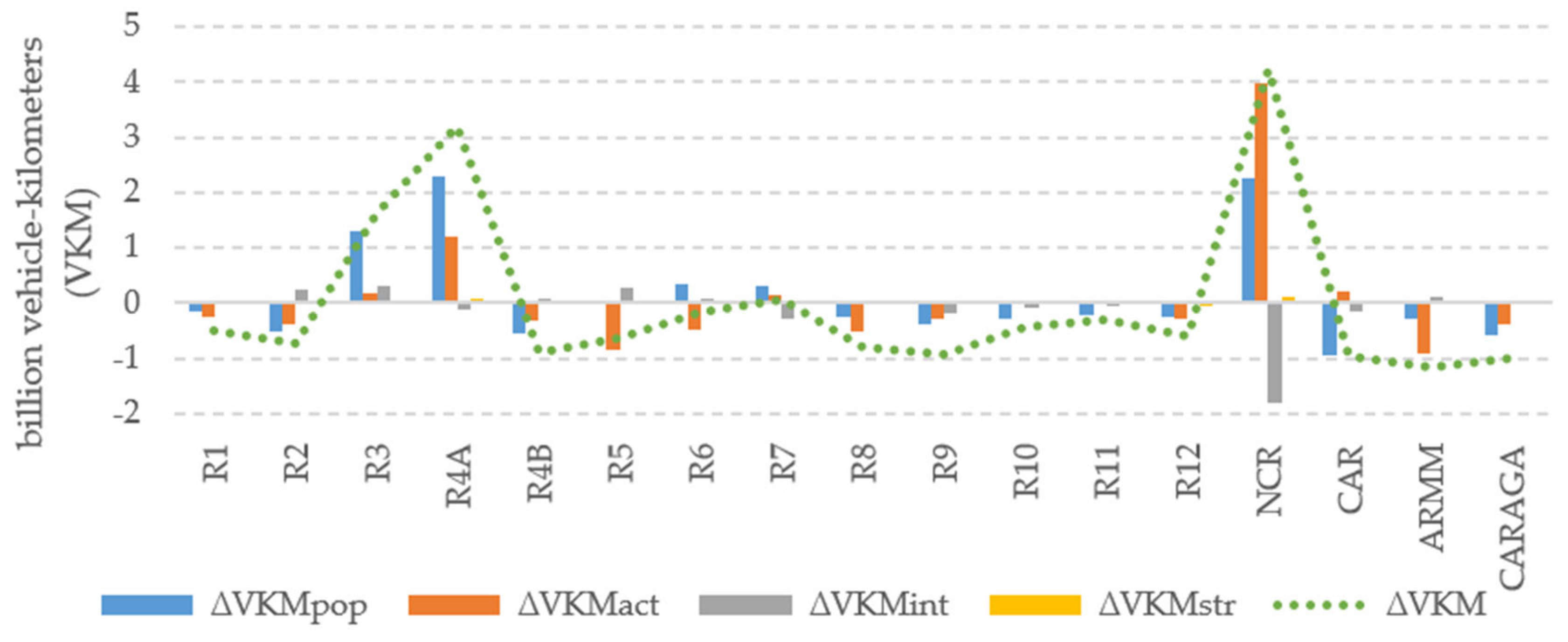
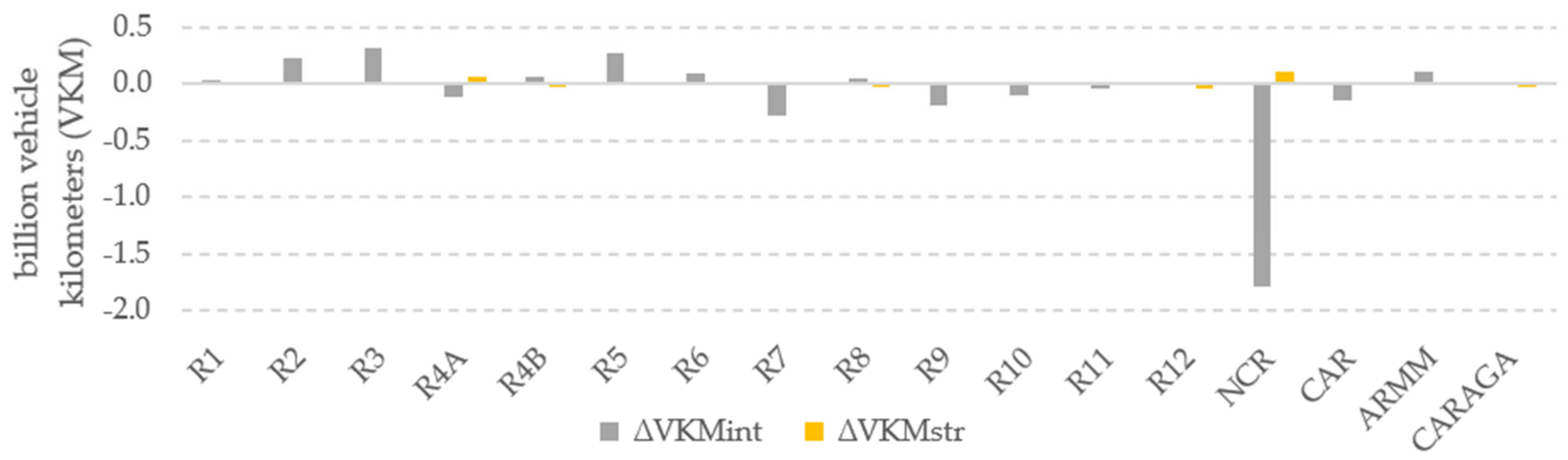
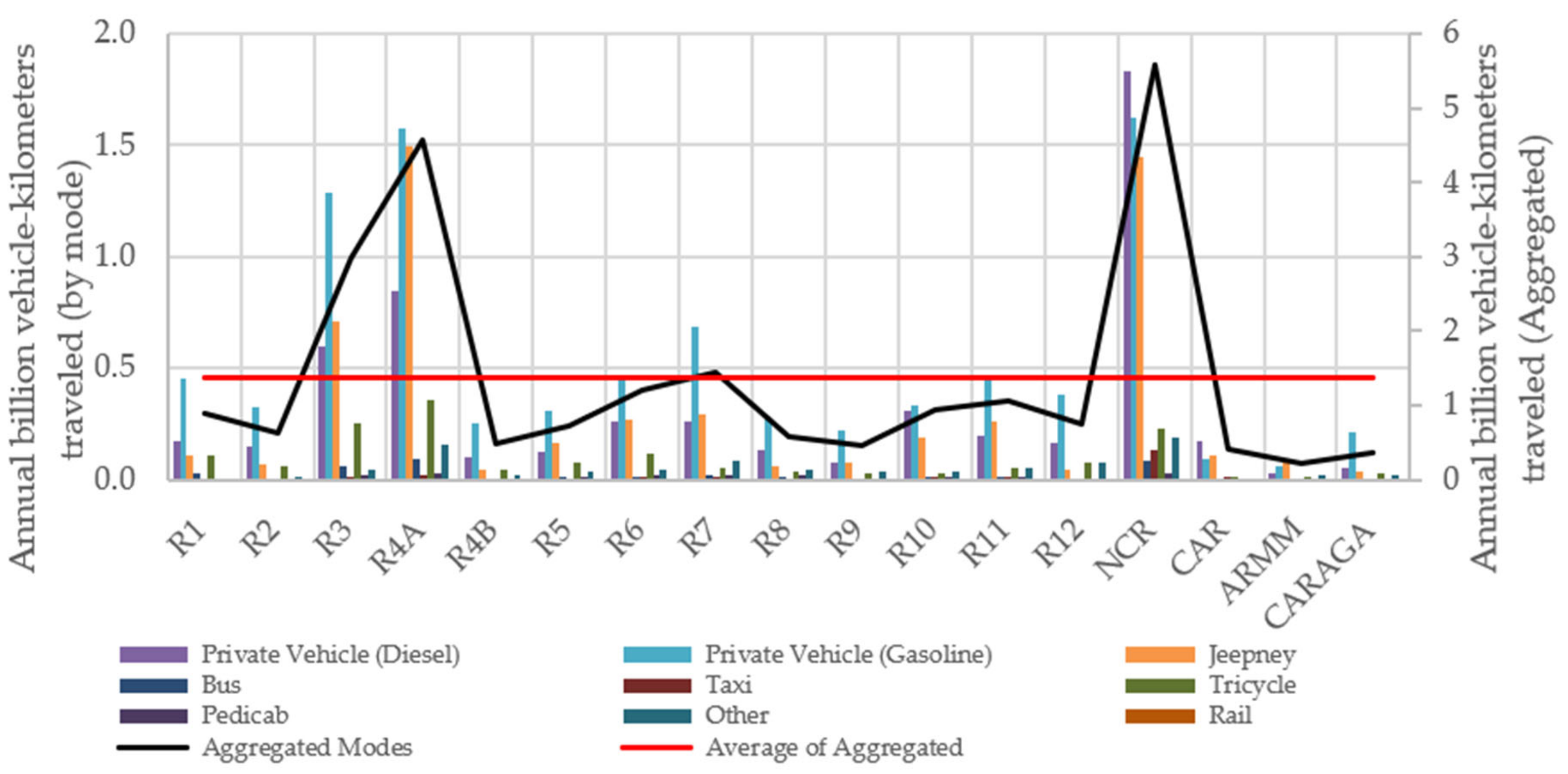
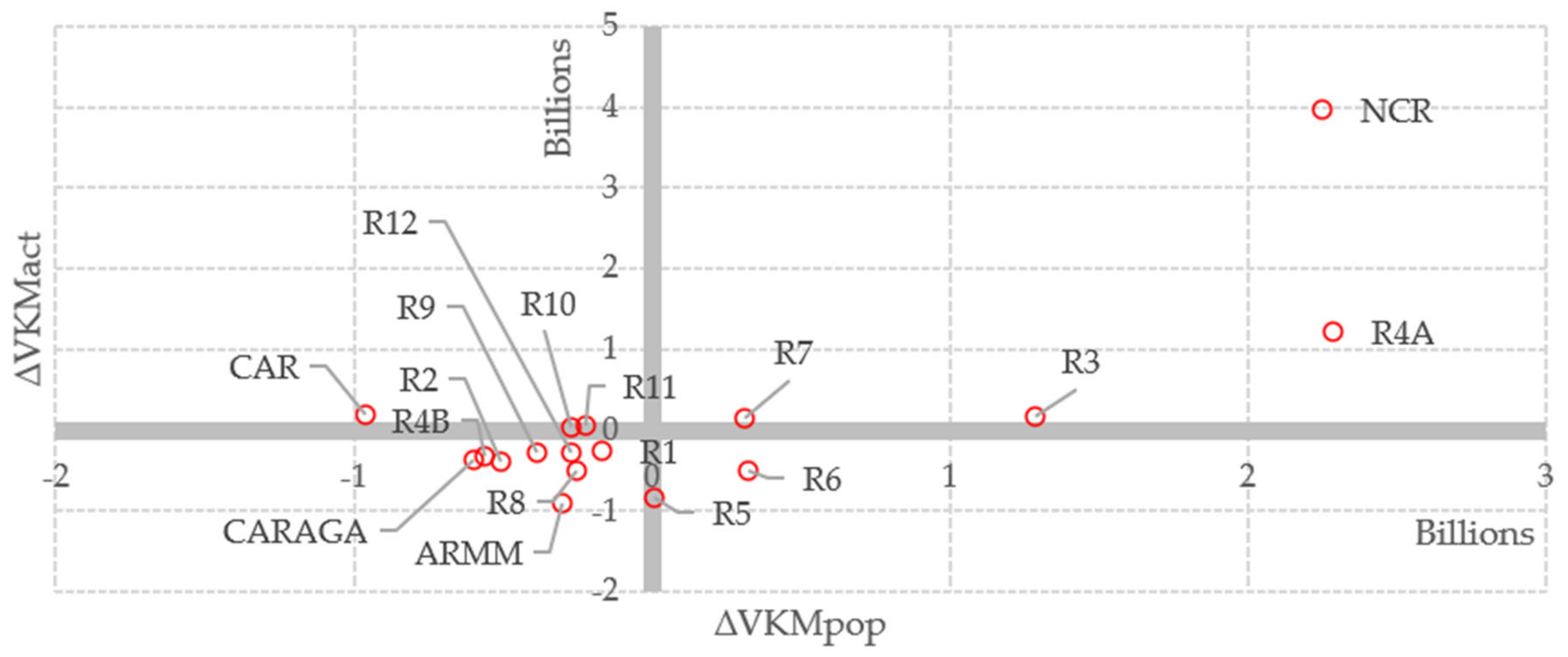
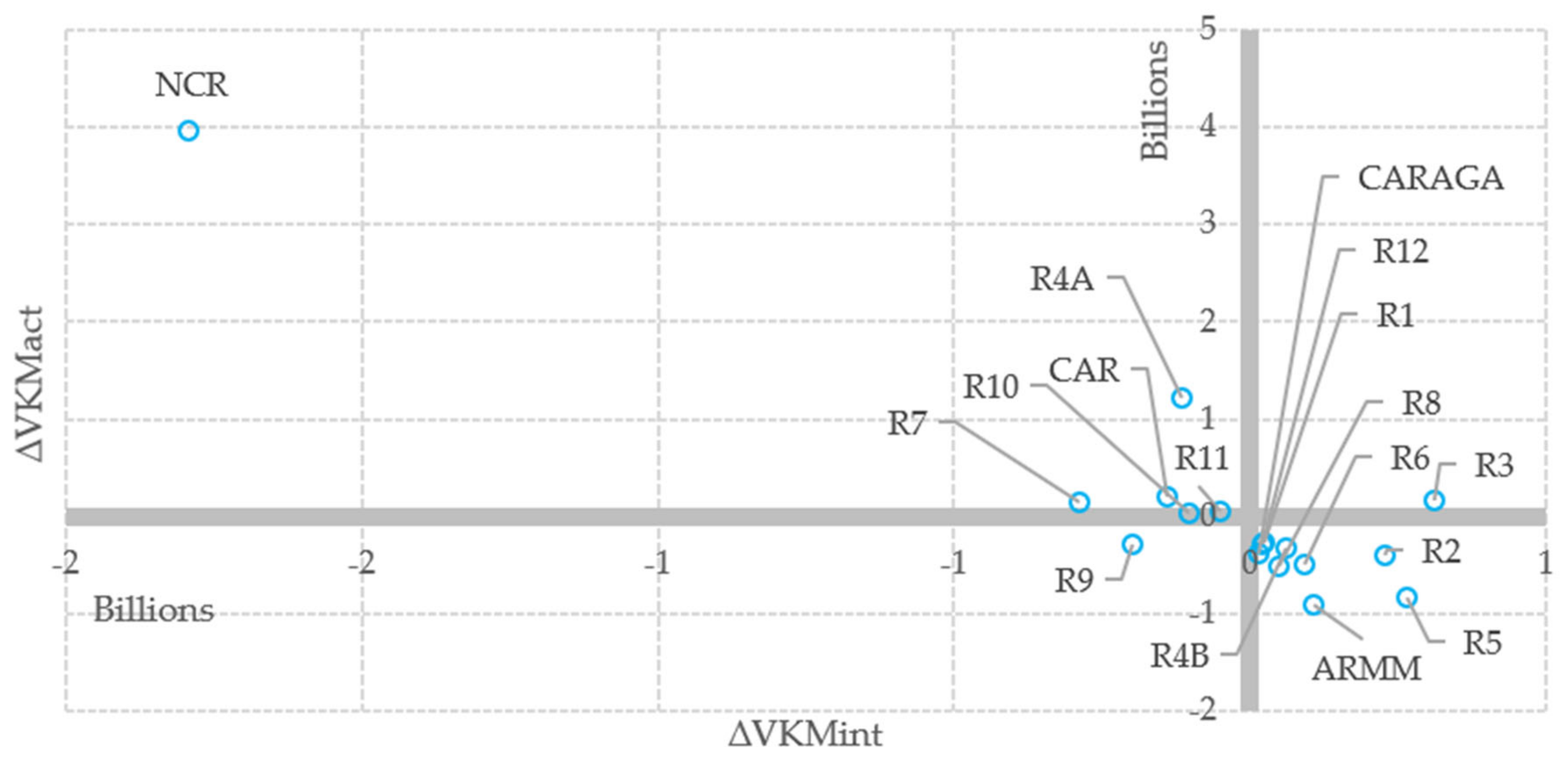
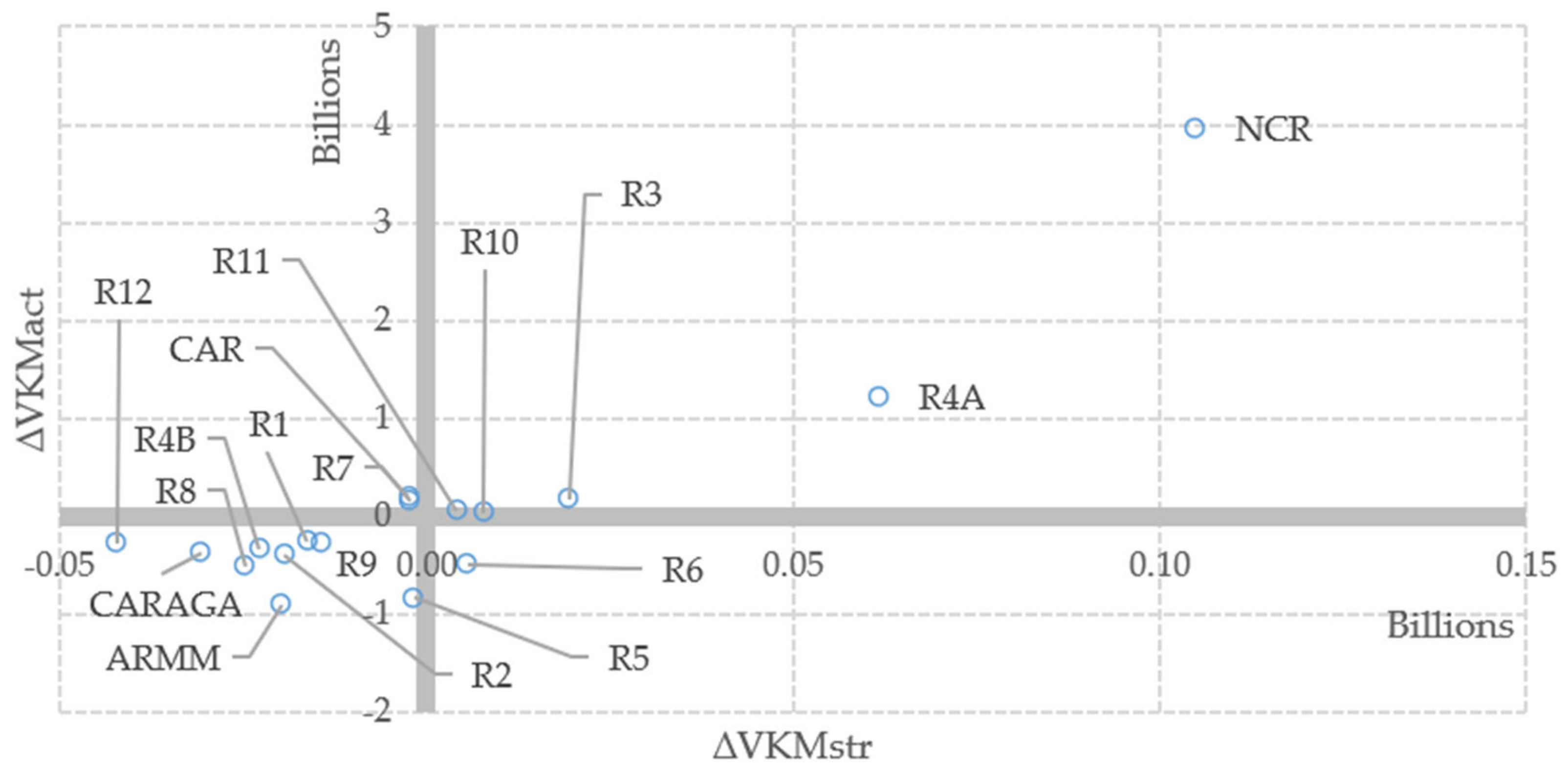
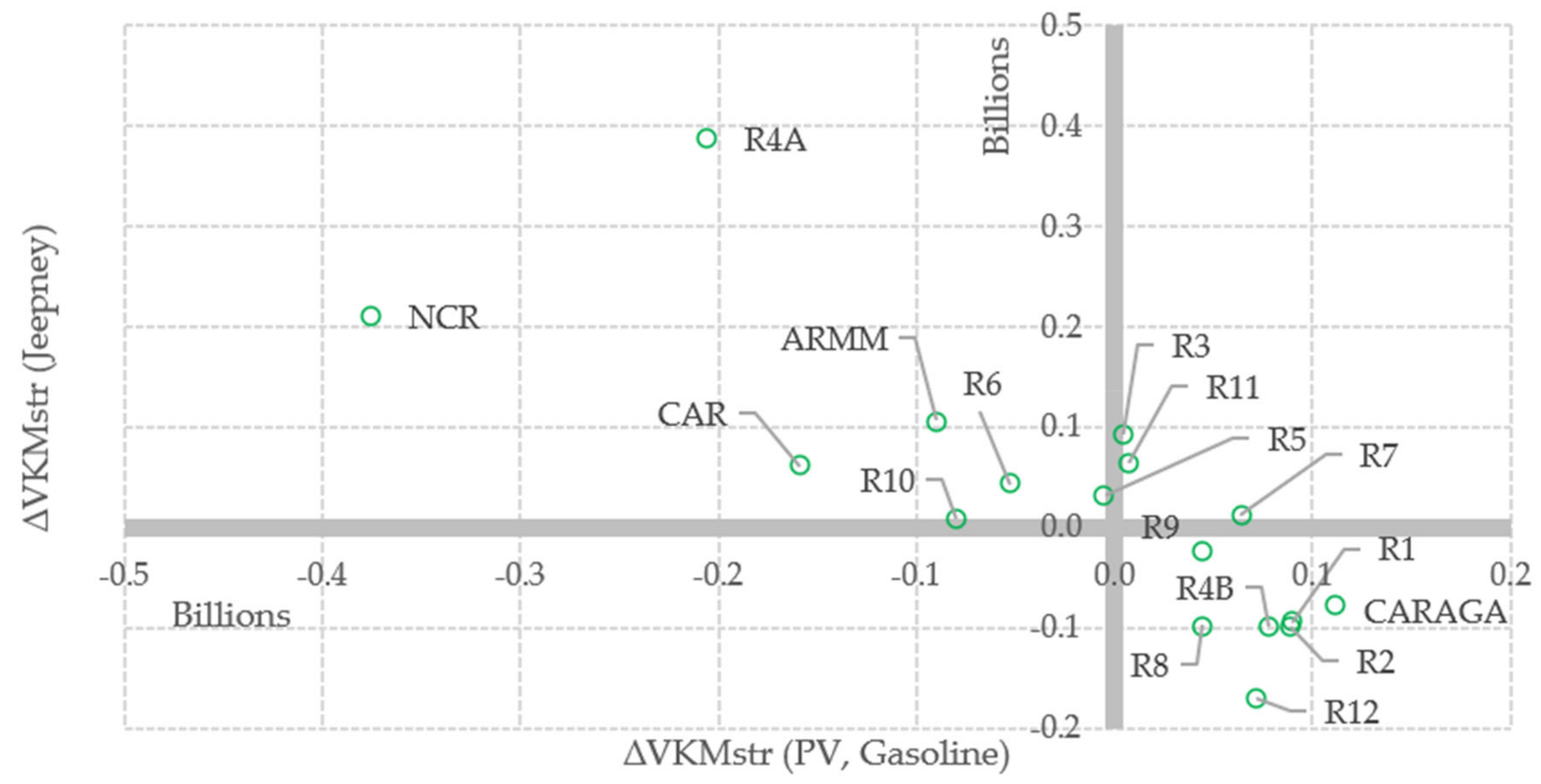
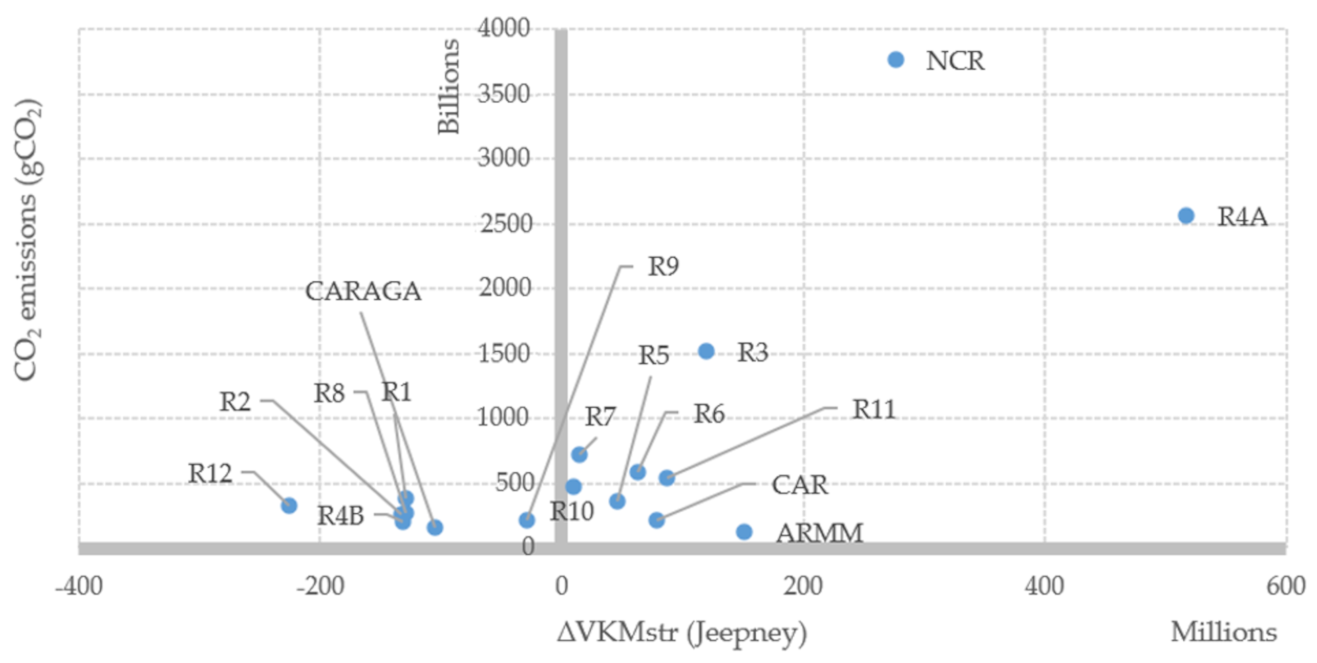
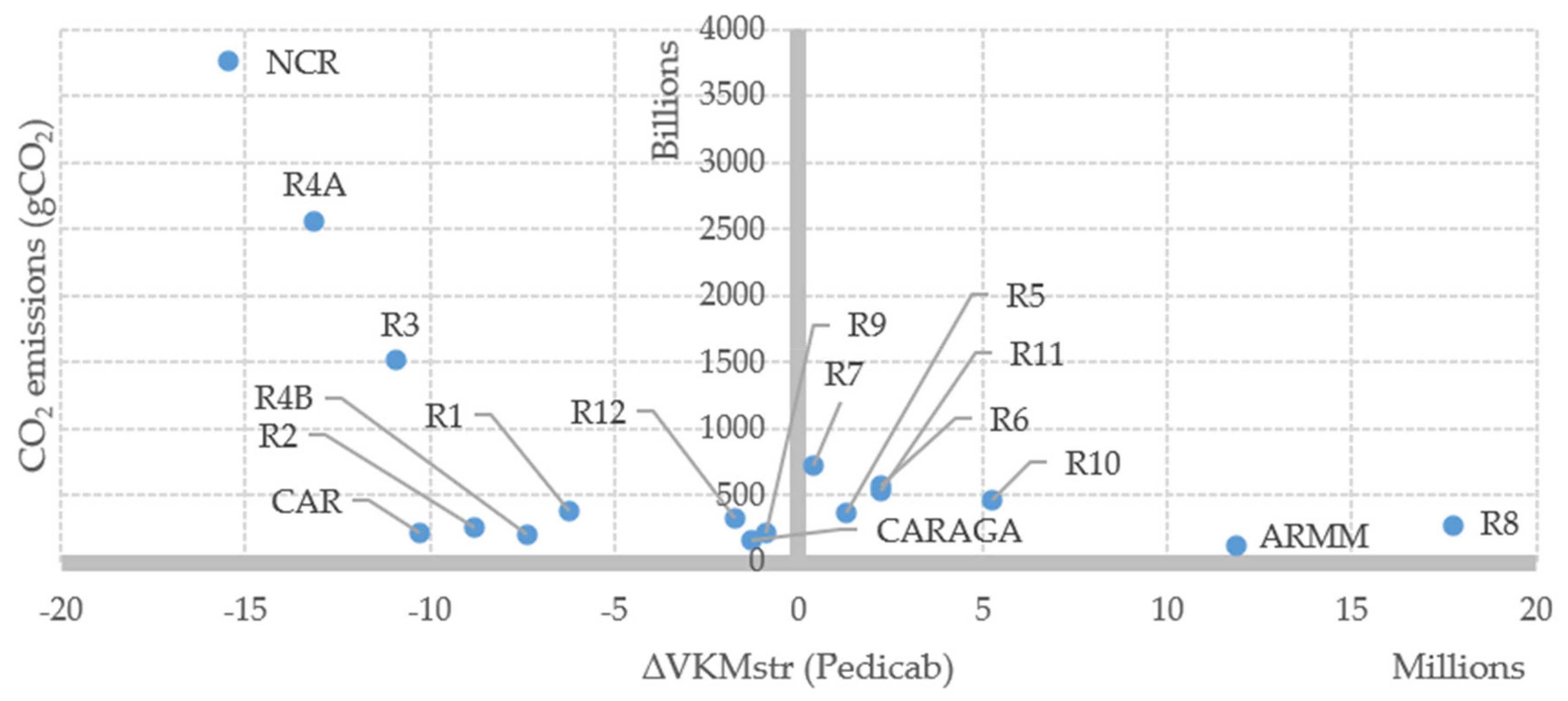
4.1. Drivers to Traffic Flow

The results of the spatial LMDI calculations are illustrated in Figure 3. Each effect (e.g., ∆VKM_pop) is represented by a column. The total difference (∆VKM) between a particular region’s VKM and the national average VKM is also plotted using a dotted line. On this chart, a positive value means that the additional VKM due to the specific effect (e.g., population growth for ∆VKM_pop) is higher than the national average and vice versa. Similarly, a negative value for the total difference (∆VKM) means that the total VKM in that region is less than the national average. As can be seen in the figure, only Regions 3, 4A, NCR and 7 (marginally) produce a VKM higher than the national average. This demonstrates one of the issues brought up in Ang [21] on the creation of a hypothetical benchmark region using the average of all other regions. If a few regions dominate the other regions, they can skew the characteristics of the benchmark region towards them.

Regions 3, 4A and NCR stand out among others in terms of vehicle-kilometers traveled per year. NCR is the economic capital of the country, while Regions 3 and 4A are directly adjacent to the north and south, respectively. Thus, it is understandable how the transport activity from NCR easily dissipates to them. It is quite common for Region 3 and 4A residents to find employment inside NCR.

With regards to the effects, it is interesting to note that population growth is the primary driver in most regions, with exception of Regions 1, 5, 6, 8, 12, ARMM and NCR, which are driven by economic activity. In Figure 4, the intensity and structural effects are presented separately. It is seen that structural effects are negligible compared to all other effects, suggesting that the difference in modal structure across regions does not significantly vary. On the other hand, it is interesting to note that NCR has a very low transport intensity. This can be explained by the fact that the majority of the major mass transport projects have been funneled into the capital and the booming high-rise residential building development in it, which created multiple mixed-use districts [45,46]. Mixed-use development can lead to reduced traveling since persons can live near their places of employment [47].

Figure 5 breaks down the total VKM by mode. While the gasoline private car dominates in most regions, it is only second to the diesel private car in NCR. This can be because of various reasons, which include the NCR residents’ higher capacity to pay, since diesel variants are usually more expensive upfront and to maintain than their gasoline counterparts and regional differences in pump oil prices. The total VKM traveled by the Jeepney (i.e., traditional open-air, minibus-type public transport vehicle) is most significant in Regions 4A and NCR. Across all regions, private vehicles and jeepneys dominate land transport.

Insights from Polar Plots: Traffic Flow

The activity effect was plotted against other effects and returned interesting trends. First, the economic activity effect (∆VKM_act) was plotted against the population effect (∆VKM_pop) in Figure 6. The scatterplot reveals an increasing trend suggesting that both contribute positively to traffic flow. Understandably, as income levels rise, vehicle ownership also rises [48] and as the population increases, the demand for additional transport also increases.

However, if a trendline is fitted with the data, an asymptotic curve can be imagined, suggesting that a saturation point can be reached. This is when further population growth in a region can no longer contribute to additional traffic flow.

Economic activity (∆VKM_act) is plotted against traffic intensity (∆VKM_int) in Figure 7. As the additional traffic flow from economic activity increases, it is observed that the traffic intensity decreases. Notably, NCR is on the far left of this scatterplot, and as explained in the earlier sub-section, this is possibly because of the fact that most major land transport infrastructure projects are concentrated in NCR. Furthermore, a variety of transport options are more abundant in NCR than in other regions. For example, there are city buses, shuttle vehicles (i.e., UV Express) and taxi services in NCR, while there are none in most regions. On the other hand, in general, the trend suggests that as the economies of each region grow, they become less traffic-intensive. Another possible explanation is that the people have a minimum and maximum need to travel. At the minimum, people need to go to work, or to school and to go home. The maximum travel need is limited by the hours of the day (i.e., you cannot travel forever in the day, there is a certain limit). Coincidentally, the high traffic intensity regions seem to be the lower-income regions (e.g., Regions 2 and 5) and the low traffic intensity regions are the high-income regions (e.g., NCR, Regions 7 and 4A). As traffic intensity is the ratio of traffic flow to GDP, a significant increase in GDP can make this quantity very small and vice versa. However, it is quite alarming that Region 3 is both on the positive axes of economic activity and traffic intensity. This suggests that if not controlled, the region is heading in an unsustainable direction.

The economic activity effect (∆VKM_act) is plotted against the structural effect (∆VKM_str) in Figure 8. While the traffic intensity tends to decrease as the economic activity increases (see Figure 7), it results in a shift to less efficient modes. It has to be noted though that the additional traffic flow due to structural effects is quite negligible compared to other effects.

The economic activity effect (∆VKM_act) is plotted against the structural effect due to private diesel vehicles (∆VKM_str (PV, Diesel)) in Figure 9. The trend shows that as the income levels increase, the population tends to shift to private diesel vehicles. This can be due to a variety of factors, which include the higher capacity to pay. This can also be an indication of the high sensitivity of the population to pump oil prices. However, it is important to note that this is not true for Region 4A. Region 4A used to enjoy lower gasoline pump prices due to the presence of a refinery in the region.

Finally, the structural effect due to jeepneys (∆VKM_str (Jeepney)) was plotted against the structural effect due to private gasoline vehicles (∆VKM_str (PV, Gasoline)) in Figure 10. The plot shows an interesting trend wherein as the percentage share of jeepney traffic increases, the percentage share of private gasoline vehicle traffic decreases. This suggests that private gasoline vehicle trips are the ones substituted for jeepney trips and vice versa.

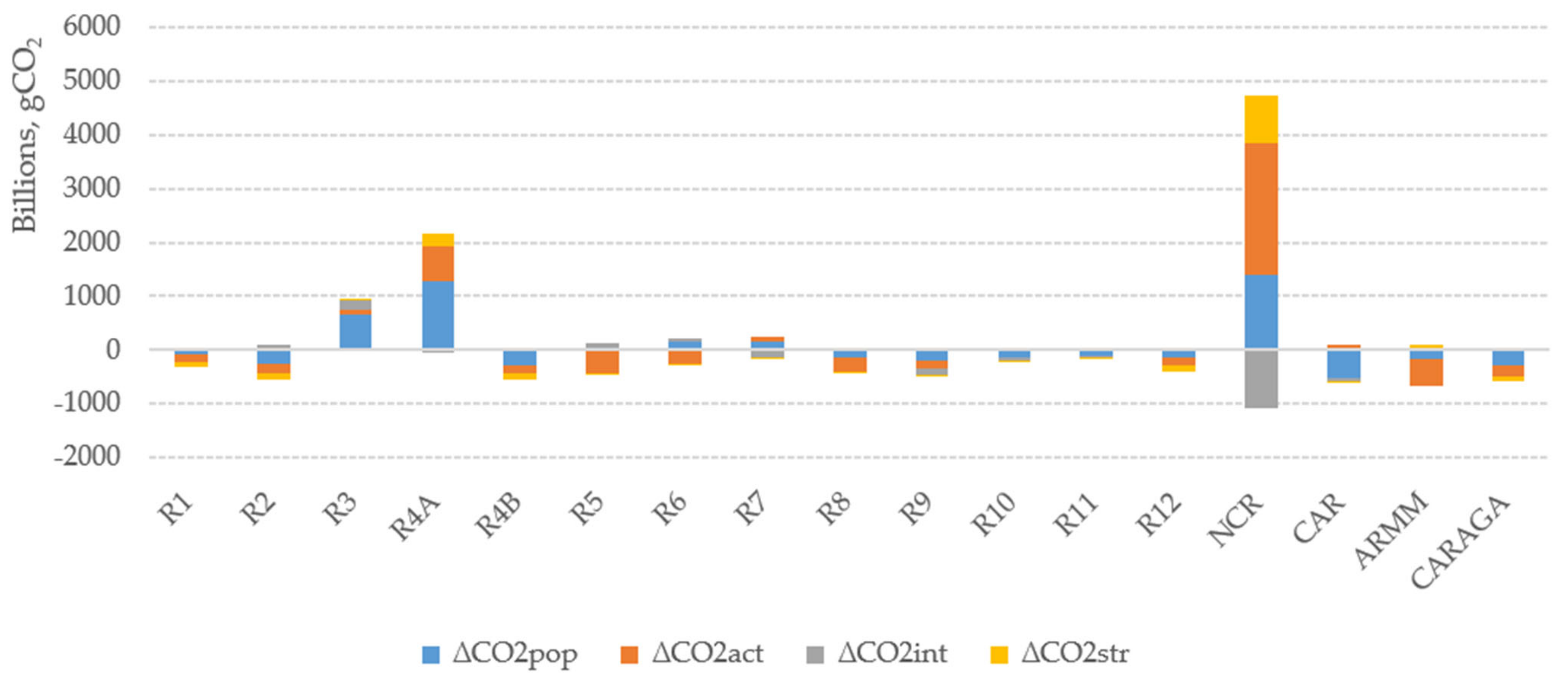
4.2. Drivers of Transport Emissions

Comparing the scatterplots for both traffic flow and transport emissions, the trends are generally similar (i.e., the same drivers that cause the increase in traffic flow are responsible for the increase in emissions). This is not surprising, because a majority of the transportation in the Philippines is fossil powered. As the authors reflected on this, unique drivers can only be observed if a significant portion of the transport activity is active (e.g., biking) or from renewables (e.g., electric vehicles charged using renewables). However, this does not mean there are no other interesting results from this portion of the study. Other notable findings are discussed below.

In the Philippines, as the results suggest, switching to public transport does not ultimately reduce emissions. As shown in Figure 11, increasing public transport share does not show a significant decrease in transport emissions. What this suggests is that the increasing public transport share is just a spillover from private transport, that is, if people can travel by private modes, they will. The need is to reduce the total VKM or to switch to cleaner energy sources for transport. However, switching to cleaner energy sources does not guarantee that emissions will be reduced because of the concept of induced demand. As shown in previous literature, the concept of using cleaner, more sustainable sources can encourage the public to travel and to consume more. While promoting alternatively powered vehicles, it is also important to take note that electric vehicles would also depend on the electricity grid mix. An electricity grid reliant on fossil power will not enable electric vehicles to meet their full potential with regards to mitigating carbon emissions.

Another interesting observation is that regions with high transport emissions tend to have very low active transport activity (see Figure 12). However, increasing active transport does not seem to reverse this, or affect emissions significantly. Reflecting on this, this can be because there are practical limits to active transport, that is, not everyone can bike or walk to work since it entails a level of physical fitness. Also, regions with high transport emissions tend to be more urbanized and spread out, further discouraging the practicality of biking or walking. Moreover, the weather is a big factor especially in a tropical country like the Philippines. With that in mind, policymakers should temper the promotion of active transport with regards to reducing carbon emissions. While it is helpful to some extent, from a larger perspective, it is not the solution that is needed. On the other hand, Banister [47] argues the important role played by mixed-use development in the sustainable mobility paradigm. In the national capital region of the Philippines, mixed-use development areas are on the rise. These are districts that combine residential, commercial and business areas in one place, for example, Bonifacio Global City, Eastwood City and Filinvest City. This connects to active transport, as one key feature of mixed-use development is the reduction of the daily commute distance, making biking or walking more practical to everybody.

Analyzing a stacked column of transport emission drivers across regions (see Figure 13), some key observations were also found. For Regions 3 and 4A, the main driver is population growth, while for NCR, the main driver is economic activity. This shows the developmental evolution of a region in the Philippines. Since Regions 3 and 4A are directly adjacent to NCR, it can be assumed that the development is more of a spillover from the national capital, NCR. To address this, more aggressive decentralization should be strategized by the government, so as not to sacrifice the sustainability of Regions 3 and 4A. In a few years, both might become as unsustainable as NCR, if not controlled. Regions way up north and down south need to be developed rapidly to control the unsustainable growth of Regions 3, 4A and NCR. Furthermore, it can be observed that while NCR has a low travel intensity, the sheer size of its economic activity significantly drives its transport emissions upwards. Thus, in the national capital, it is more of an over-demand problem than a technology problem. Also, it is alarming that Region 3 is showing an unsustainable trend, with both a positive transport intensity effect and economic activity effect. This suggests a strong need to improve public transport infrastructure in the region, as recommended in [6].

5. Conclusions and Way Forward

The bottom line of this study is to reduce the need to travel. This is highly relevant considering how the recent pandemic has affected mobility. In an instant, the world had learned to adapt to telecommuting, as global lockdowns were put in place. In April 2020, up to 90% of cities worldwide were in lockdown at a particular point in time [49]. With regards to increasing traffic flow and emissions from transport, it deserves to be contemplated that technological innovation might not be the key but behavioral change. In a way, sound urban planning can also reduce the need to travel.

Transportation is responsible for almost 30% of global CO₂ emissions, and this growth is largely because of increasing dependence on private vehicles. This study demonstrated the potential of using spatial decomposition in the early diagnosis of traffic flow problems in regions. By comparing regions with each other, the cause for increasing or decreasing traffic flow and transport emissions can be determined and ideas can be tested. For example, as shown in the paper, increasing public transport share did not result in reduced transport emissions, nor did increasing active transport share. Using spatial decomposition analysis, potential driving factors are not merely determined. Instead, their individual contributions to traffic flow and emissions are compared with one another to show the potential effect of growth in a certain region. A new tool is explored by this paper that can help in the mitigation of worsening traffic flows and emissions in regions. However, in future studies, a better way to define the hypothetical benchmark region needs to be explored.

The following policy recommendations arising from the results of this paper can be further investigated:

• Equity on the distribution of transport infrastructure projects. The government needs to invest in mass transport services outside NCR to reduce the dependence of other regions on private vehicle modes. This can accelerate the decentralization of growth to other regions up north and down south. While these regions’ shares in traffic flow are not yet significant, the current situation could be leading them toward an unsustainable and irreversible route. The results of this study support the increased taxation of new private vehicle purchases; however, the authors advocate that revenues from these new taxes have to be reinvested in the development of quality public transport services.
• Improve the quality of public transport services. The data showed that jeepney trips are substituted for private gasoline vehicle trips and vice versa. As income levels rise, people grab the opportunity to own private vehicles. This is understandable especially if the quality of public transport services is unbearable. The population deserves a decent means to go to work, to school, etc., and it should be a priority of the government. In fact, the national government of the Philippines had been pushing for the jeepney modernization program, but however, social and cultural issues have delayed its implementation.
• Support telecommuting. The improvement of public transport services goes hand in hand with the reduction of the demand for it. As shown by the data in this study, increasing public transport share does not ultimately result in lower transport emissions. At the end of the day, reducing transport demand is the key. The government should find ways to support and encourage employers who successfully adapted telecommuting in their operations to significantly reduce transport demand.
• Promote mixed-use development. As shown in this study, active transport does not help the reduction of transport emissions significantly, perhaps due to practical reasons. Mixed-use development decreases the commute distance and thus can encourage more biking and walking. The pursuance of active transport projects (e.g., bike lanes) has to be connected to mixed-use areas to maximize their effectiveness.

References

1. Philippine Atmospheric, Geophysical Astronomical Services Administration (PAGASA). Climate Projections in the Philippines. Climate Change in the Philippines. Available online: https://www1.pagasa.dost.gov.ph/index.php/93-cad1/472-climate-projections (accessed on 10 May 2021).
2. IPCC. Climate Change 2014: Synthesis Report. In Contribution of Working Groups I, II and III to the Fifth Assessment Report of the Intergovernmental Panel on Climate Change (IPCC); IPCC: Geneva, Switzerland, 2014. [Google Scholar]
3. IEA. CO2 emissions from fuel combustion. Int. Energy Agency 2016, 533. [Google Scholar] [CrossRef]
4. International Energy Agency Global Energy & CO2 Status Report; Paris. 2019. Available online: https://www.iea.org/reports/global-energy-co2-status-report-2019 (accessed on 13 May 2021).
5. The World Bank. Urban Transport and Climate Change. Available online: https://www.worldbank.org/en/news/feature/2012/08/14/urban-transport-and-climate-change (accessed on 5 May 2021).
6. Lopez, N.S.; Chiu, A.S.F.; Biona, J.B.M. Decomposing drivers of transportation energy consumption and carbon dioxide emissions for the Philippines: The case of developing countries. Front. Energy 2018, 12, 389–399. [Google Scholar] [CrossRef]
7. Wu, H.M.; Xu, W. Cargo transport energy consumption factors analysis: Based on LMDI decomposition technique. IERI Procedia 2014, 9, 168–175. [Google Scholar] [CrossRef] [Green Version]
8. Chen, L.; Yang, Z. A spatio-temporal decomposition analysis of energy-related CO2 emission growth in China. J. Clean. Prod. 2015, 103, 49–60. [Google Scholar] [CrossRef]
9. Dargay, J.; Gately, D. Income’s effect on car and vehicle ownership, worldwide: 1960–2015. Transp. Res. Part A Policy Pract. 1999, 33, 101–138. [Google Scholar] [CrossRef]
10. Martin, E.; Shaheen, S.A.; Lidicker, J. Impact of carsharing on household vehicle holdings: Results from North American shared-use vehicle survey. Transp. Res. Rec. 2010, 2143, 150–158. [Google Scholar] [CrossRef]
11. Ubando, A.T.; Gue, I.H.; Rith, M.; Gonzaga, J.; Lopez, N.S.; Biona, J.B. A systematic approach to the optimal planning of energy mix for electric vehicle policy. Chem. Eng. 2019, 76. [Google Scholar] [CrossRef]
12. Papagiannaki, K.; Diakoulaki, D. Decomposition analysis of CO2 emissions from passenger cars: The cases of Greece and Denmark. Energy Policy 2009, 37, 3259–3267. [Google Scholar] [CrossRef]
13. Jiang, J. A factor decomposition analysis of transportation energy consumption and related policy implications. IATSS Res. 2015, 38, 142–148. [Google Scholar] [CrossRef] [Green Version]
14. Ding, J.; Jin, F.; Li, Y.; Wang, J.E. Analysis of transportation carbon emissions and its potential for reduction in China. Chin. J. Popul. Resources Environ. 2013, 11, 17–25. [Google Scholar] [CrossRef] [Green Version]
15. Wang, Y.; Hayashi, Y.; Kato, H.; Liu, C. Decomposition analysis of CO2 emissions increase from the passenger transport sector in Shanghai, China. Int. J. Urban Sci. 2011, 15, 121–136. [Google Scholar] [CrossRef]
16. Guo, B.; Geng, Y.; Franke, B.; Hao, H.; Liu, Y.; Chiu, A. Uncovering China’s transport CO2 emission patterns at the regional level. Energy Policy 2014, 74, 134–146. [Google Scholar] [CrossRef]
17. Ang, B.W.; Zhang, F.Q.; Choi, K.H. Factorizing changes in energy and environmental indicators through decomposition. Energy 1998, 23, 489–495. [Google Scholar] [CrossRef]
18. Ang, B.W. Decomposition analysis for policymaking in energy: Which is the preferred method? Energy Policy 2004, 32, 1131–1139. [Google Scholar] [CrossRef]
19. Lopez, N.S.; Mousavi, B.; Biona, J.B.; Chiu, A.S. Decomposition Analysis of CO2 Emissions with Emphasis on Electricity Imports and Exports: EU as a Model for ASEAN Integration. Chem. Eng. Trans. 2017, 61, 739–744. [Google Scholar] [CrossRef]
20. Ang, B.W. The LMDI approach to decomposition analysis: A practical guide. Energy Policy 2005, 33, 867–871. [Google Scholar] [CrossRef]
21. Ang, B.W. LMDI decomposition approach: A guide for implementation. Energy Policy 2015, 86, 233–238. [Google Scholar] [CrossRef]
22. Feng, C.; Sun, L.X.; Xia, Y.S. Clarifying the “gains” and “losses” of transport climate mitigation in China from technology and efficiency perspectives. J. Clean. Prod. 2020, 263, 121545. [Google Scholar] [CrossRef]
23. Sorrell, S.; Lehtonen, M.; Stapleton, L.; Pujol, J.; Champion, T. Decomposing road freight energy use in the United Kingdom. Energy Policy 2009, 37, 3115–3129. [Google Scholar] [CrossRef]
24. Lu, I.J.; Lin, S.J.; Lewis, C. Decomposition and decoupling effects of carbon dioxide emission from highway transportation in Taiwan, Germany, Japan and South Korea. Energy Policy 2007, 35, 3226–3235. [Google Scholar] [CrossRef]
25. Kwon, T.H. Decomposition of factors determining the trend of CO2 emissions from car travel in Great Britain (1970–2000). Ecol. Econ. 2005, 53, 261–275. [Google Scholar] [CrossRef]
26. Liu, Y.; Feng, C. Decouple transport CO2 emissions from China’s economic expansion: A temporal-spatial analysis. Transp. Res. Part D Transp. Environ. 2020, 79, 102225. [Google Scholar] [CrossRef]
27. Andreoni, V. Galmarini, S. European CO2 emission trends: A decomposition analysis for water and aviation transport sectors. Energy 2012, 45, 595–602. [Google Scholar] [CrossRef]
28. Timilsina, G.R.; Shrestha, A. Factors affecting transport sector CO2 emissions growth in Latin American and Caribbean countries: An LMDI decomposition analysis. Int. J. Energy Res. 2009, 33, 396–414. [Google Scholar] [CrossRef]
29. Zhang, K.; Liu, X.; Yao, J. Identifying the driving forces of CO2 emissions of China’s transport sector from temporal and spatial decomposition perspectives. Environ. Sci. Pollut. Res. 2019, 26, 17383–17406. [Google Scholar] [CrossRef]
30. Tu, M.; Li, Y.; Bao, L.; Wei, Y.; Orfila, O.; Li, W.; Gruyer, D. Logarithmic Mean Divisia Index Decomposition of CO2 Emissions from Urban Passenger Transport: An Empirical Study of Global Cities from 1960–2001. Sustainability 2019, 11, 4310. [Google Scholar] [CrossRef] [Green Version]
31. Cao, X.; OuYang, S.; Liu, D.; Yang, W. Spatiotemporal Patterns and Decomposition Analysis of CO2 Emissions from Transportation in the Pearl River Delta. Energies 2019, 12, 2171. [Google Scholar] [CrossRef] [Green Version]
32. Feng, C.; Xia, Y.S.; Sun, L.X. Structural and social-economic determinants of China’s transport low-carbon development under the background of aging and industrial migration. Environ. Res. 2020, 188, 109701. [Google Scholar] [CrossRef]
33. Li, W.; Li, H.; Zhang, H.; Sun, S. The analysis of CO2 emissions and reduction potential in China’s transport sector. Math. Probl. Eng. 2016, 2016. [Google Scholar] [CrossRef] [Green Version]
34. Lian, L.; Lin, J.; Yao, R.; Tian, W. The CO 2 emission changes in China’s transportation sector during 1992–2015: A structural decomposition analysis. Environ. Sci. Pollut. Res. 2020, 1–4. [Google Scholar] [CrossRef]
35. Román-Collado, R.; Morales-Carrión, A.V. Towards a sustainable growth in Latin America: A multiregional spatial decomposition analysis of the driving forces behind CO2 emissions changes. Energy Policy 2018, 115, 273–280. [Google Scholar] [CrossRef]
36. Timilsina, G.R.; Shrestha, A. Transport sector CO2 emissions growth in Asia: Underlying factors and policy options. Energy policy 2009, 37, 4523–4539. [Google Scholar] [CrossRef]
37. Mendiluce, M.; Schipper, L. Trends in passenger transport and freight energy use in Spain. Energy Policy 2011, 39, 6466–6475. [Google Scholar] [CrossRef]
38. Shi, Y.; Han, B.; Han, L.; Wei, Z. Uncovering the national and regional household carbon emissions in China using temporal and spatial decomposition analysis models. J. Clean. Prod. 2019, 232, 966–979. [Google Scholar] [CrossRef]
39. Sumabat, A.K.; Lopez, N.S.; Yu, K.D.; Hao, H.; Li, R.; Geng, Y.; Chiu, A.S. Decomposition analysis of Philippine CO2 emissions from fuel combustion and electricity generation. Appl. Energy. 2016, 164, 795–804. [Google Scholar] [CrossRef]
40. Philippine Statistics Authority. Family Income and Expenditure Survey (FIES). 2015. Available online: https://psa.gov.ph/content/statistical-tables-2015-family-income-and-expenditure-survey (accessed on 9 March 2018).
41. Philippine Statistics Authority. The Gross Regional Domestic Product (GRDP). 2016. Available online: Psa.gov.ph/sites/default/files/2015-2017grdp%20publication.pdf (accessed on 11 March 2020).
42. Department of Energy. NCR/Metro Manila Prevailing Retail Pump Prices. Available online: https://www.doe.gov.ph/retail-pump-prices-metro-manila?ckattempt=2&fbclid=IwAR1an3gkTR8pOHqNZKb4K2JCUdJ57t1YieAWUANnx3arrnOzg0GrSFYxK5Q (accessed on 17 May 2021).
43. Land Transportation Franchising and Regulatory Board. Fare Rates. Available online: https://ltfrb.gov.ph/fare-rates/?fbclid=IwAR3dqRxhhdhGenOMr8Li4fGlMLSbUgxPJIxfVKW4BHP3zDWoZXJcKMwCfVY (accessed on 17 May 2021).
44. Fabian, H.; Gota, S. CO2 emissions from the land transport sector in the Philippines: Estimates and policy implications. In Proceedings of the 17th Annual Conference of the Transportation Science Society of the Philippines, Pasay, Philippines, 4 September 2009. [Google Scholar]
45. Tomeldan, M.V.; Antonio, M.; Arcenas, J.; Beltran, K.M.; Cacalda, P.A. “Shared Growth” Urban Renewal Initiatives in Makati City, Metro Manila, Philippines. J. Urban Manag. 2014, 3, 45–65. [Google Scholar] [CrossRef]
46. Philippine Institute for Development Studies. Land Use Planning in Metro Manila and the Urban Fringe: Implications on the Land and Real Estate Market. 2000. Available online: https://dirp3.pids.gov.ph/ris/dps/pidsdps0020.pdf (accessed on 5 January 2021).
47. Banister, D. The sustainable mobility paradigm. Transp. Policy 2008, 15, 73–80. [Google Scholar] [CrossRef]
48. Rith, M.; Roquel, K.I.; Lopez, N.S.; Fillone, A.M.; Biona, J.B. Towards more sustainable transport in Metro Manila: A case study of household vehicle ownership and energy consumption. Transp. Res. Interdiscip. Perspect. 2020, 6, 100163. [Google Scholar] [CrossRef]
49. Devi, S. Travel restrictions hampering COVID-19 response. Lancet 2020, 395, 1331–1332. [Google Scholar] [CrossRef]
Figure 1. Conceptual framework of the study.
Sustainability 13 06500 g001
Figure 2. Map of Philippines with Regions.
Sustainability 13 06500 g002
Figure 3. Effect estimates by region, as compared with the national average, μ. ∆VKMpop refers to the population effect, ∆VKMact refers to the activity effect, ∆VKMint refers to the intensity effect and ∆VKMstr refers to the structural effect.
Sustainability 13 06500 g003
Figure 4. Effect estimates by region for traffic intensity (∆VKMint) and modal structure (∆VKMstr), as compared with the national average, μ.
Sustainability 13 06500 g004
Figure 5. Breakdown of modal share by region.
Sustainability 13 06500 g005
Figure 6. Polar plot between economic activity and population. ∆VKMact and ∆VKMpop refer to the activity and population effects, respectively.
Sustainability 13 06500 g006
Figure 7. Polar plot between economic activity and traffic intensity. ∆VKMact and ∆VKMint refer to the activity and intensity effects, respectively.
Sustainability 13 06500 g007
Figure 8. Polar plot between economic activity and modal structure. ∆VKMact and ∆VKMstr refer to the activity and structural effects, respectively.
Sustainability 13 06500 g008
Figure 9. Polar plot between economic activity and modal share of private diesel vehicles. ∆VKMact and ∆VKMstr (PV, Diesel) refer to the activity effect and the structural effect of private diesel vehicles, respectively.
Sustainability 13 06500 g009
Figure 10. Polar plot between modal shares of jeepneys and private gasoline vehicles. ∆VKMstr (Jeepney) and ∆VKMstr (PV, Gasoline) refer to the structural effect of public jeepney vehicles and the structural effect of private gasoline vehicles, respectively.
Sustainability 13 06500 g010
Figure 11. Plot between CO2 emissions and effect of increasing modal share of jeepneys, ∆VKMstr (Jeepney).
Sustainability 13 06500 g011
Figure 12. Plot between CO2 emissions and effect of increasing modal share of pedicabs (i.e., pedaled tricycles), ∆VKMstr (Pedicab).
Sustainability 13 06500 g012
Figure 13. Transport emission drivers across regions.
Sustainability 13 06500 g013