
Parameter Extraction of Three Diode Solar Photovoltaic Model Using Improved Grey Wolf Optimizer


Abstract
:1. Introduction
2. Mathematical Mode and Optimization Problem
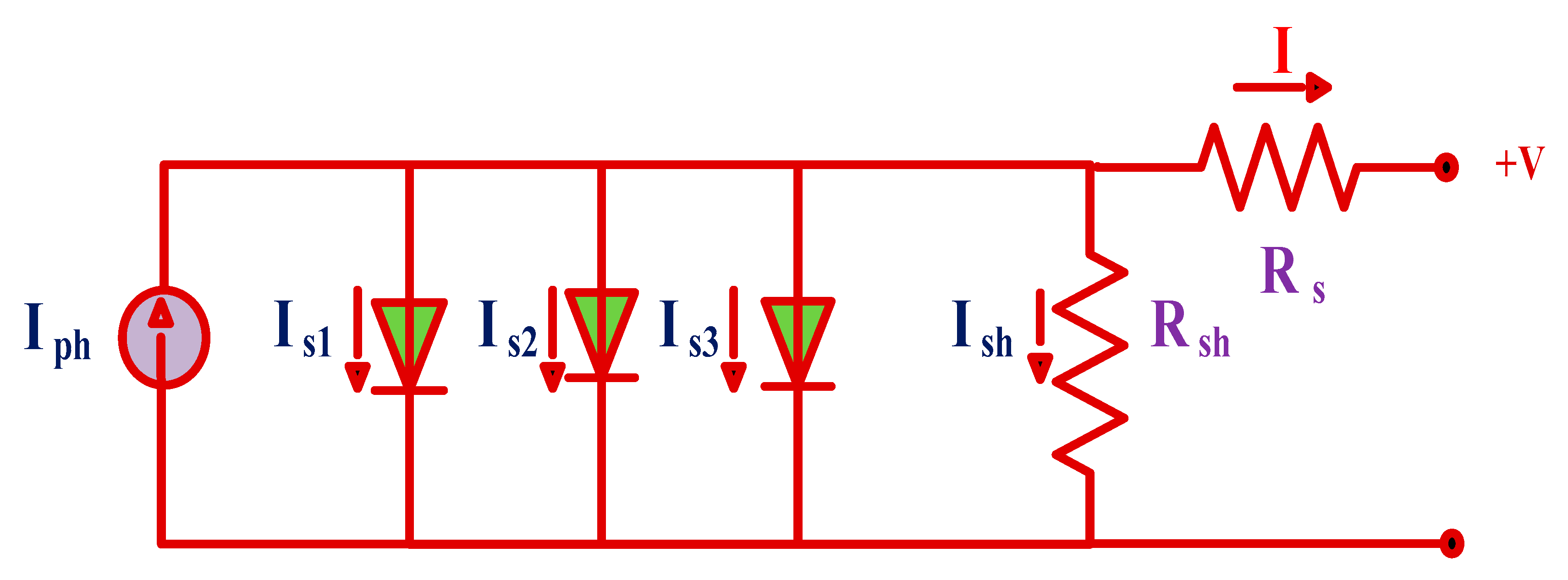
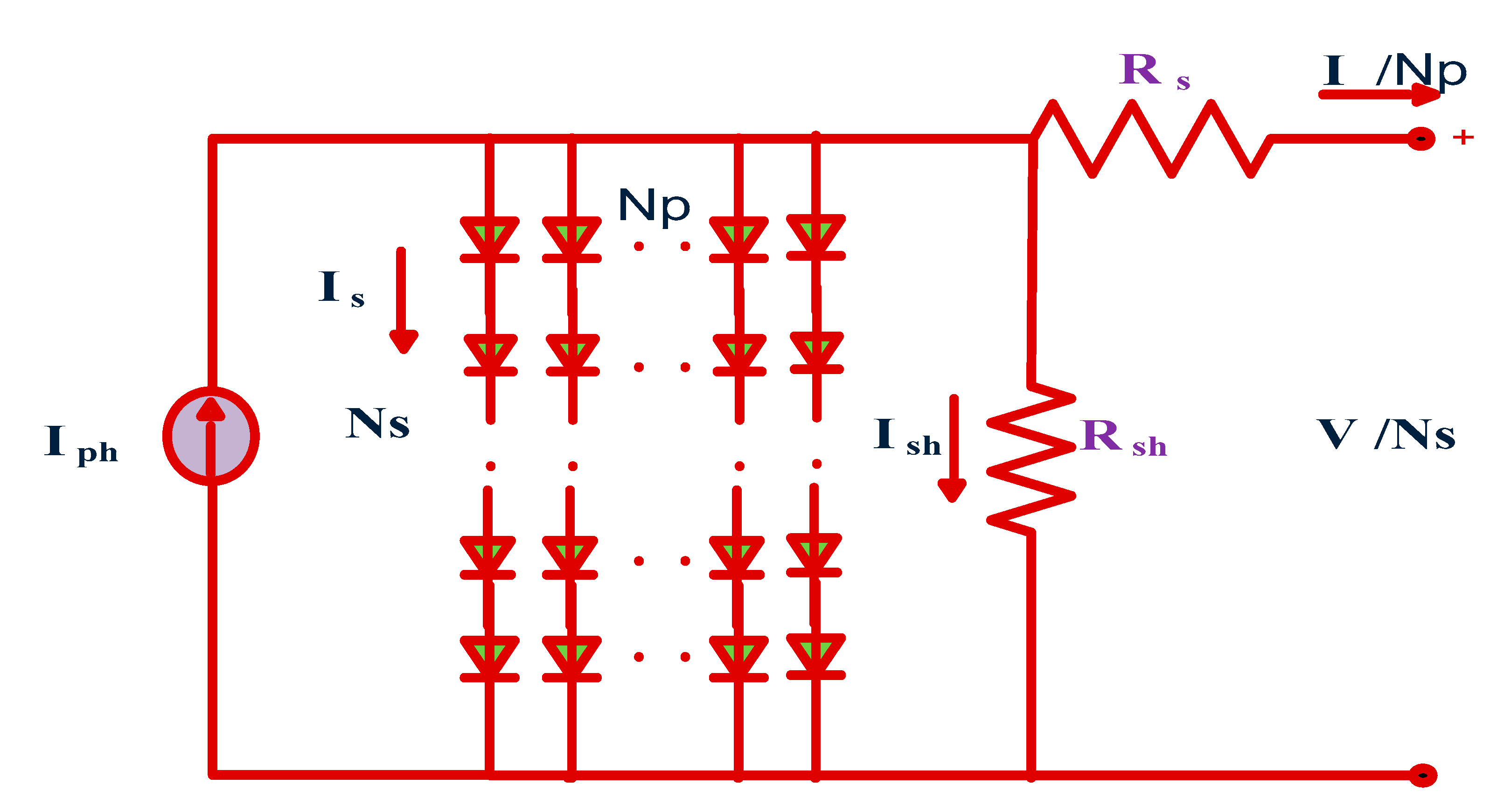
2.1. Model of TDM and PV Panel
- First diode represents the effect of diffusion current .
- First diode represents the effect of diffusion current .
- Second diode represents the effect of recombination current .
- Third diode represents the effect of grain boundaries and large leakage current .
- Series resistance represents the semiconductor material resistance at neutral regions .
- Shunt resistance represents the current leakage resistance across the P-N junction of PV system .
2.2. Objective Function
3. Grey Wolf Optimizers
3.1. Grey Wolf Optimizer (GWO)
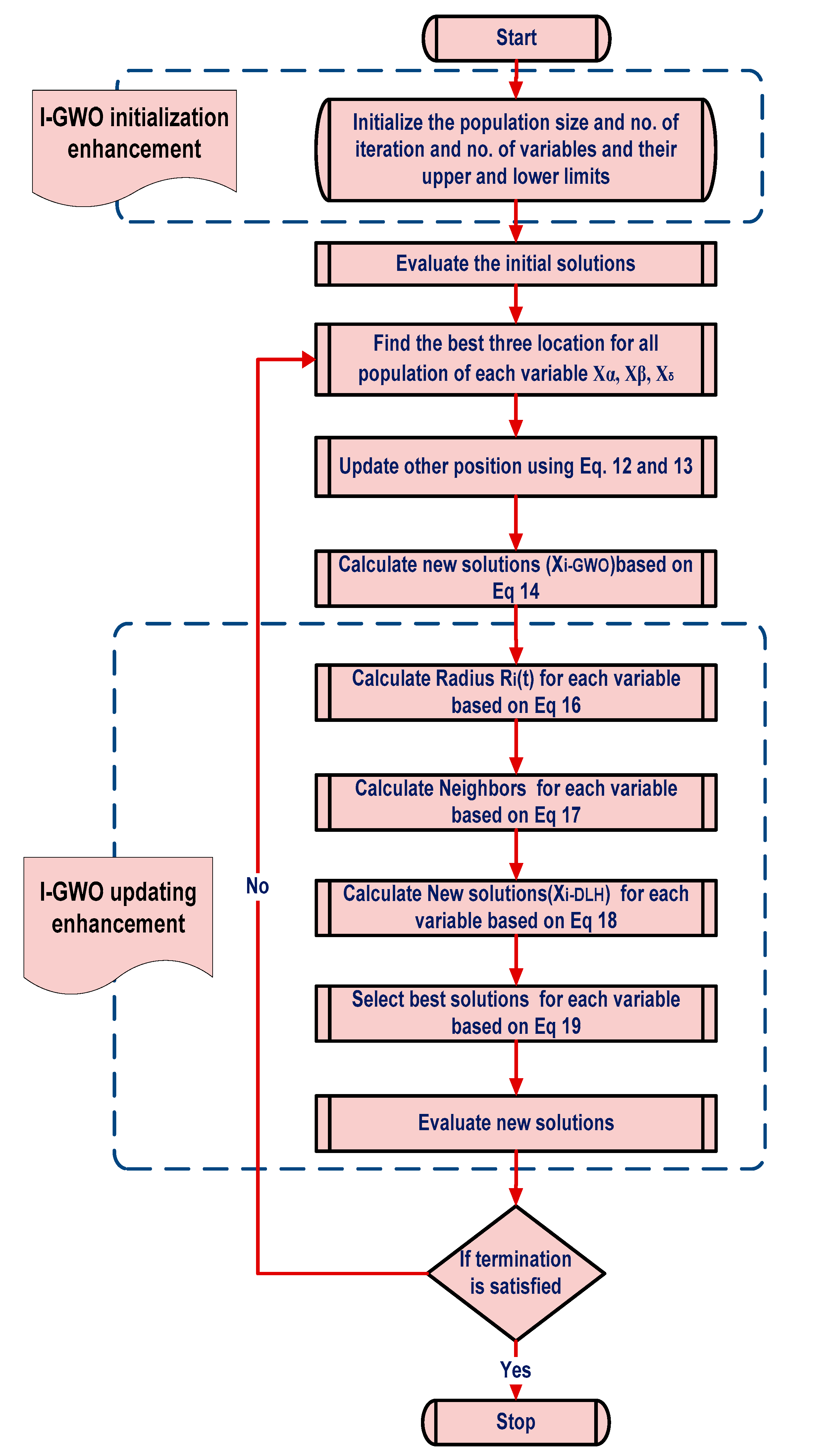
3.2. Improved Grey Wolf Optimizer (I-GWO)
- -
- Increasing the initialization by random distribution for N wolfs within the search range as described in Equation (15).where, problem dimension, problem dimension. LB and UB are the search low and upper limits, respectively.
- -
- The tracking behavior is enhanced using dimension learning-based hunting technique (DLH). In DLH, each wolf learns from its neighbors. The construction of the neighbors according to the calculated radius are calculated by Equations (16) and (17). The new positions are determined using Equation (18).
- -
- Random distribution for N wolfs within the search range, as shown by (15)
- -
- (Main steps)
- -
- For iteration = 1 to maximum iteration
- -
- Find three wolf leaders , and ,
- -
- Update three wolf leaders’ positions, and using (12) and (13).
- -
- Calculate the best position using (14)
- -
- (Updating improvement steps (DLH))
- -
- Calculate radius to construction of the neighbors using (16)
- -
- Determine the neighbors using Equation (17)
- -
- Calculate new solution using (18)
- -
- Select the best position between and using (19)
- -
- End for loop
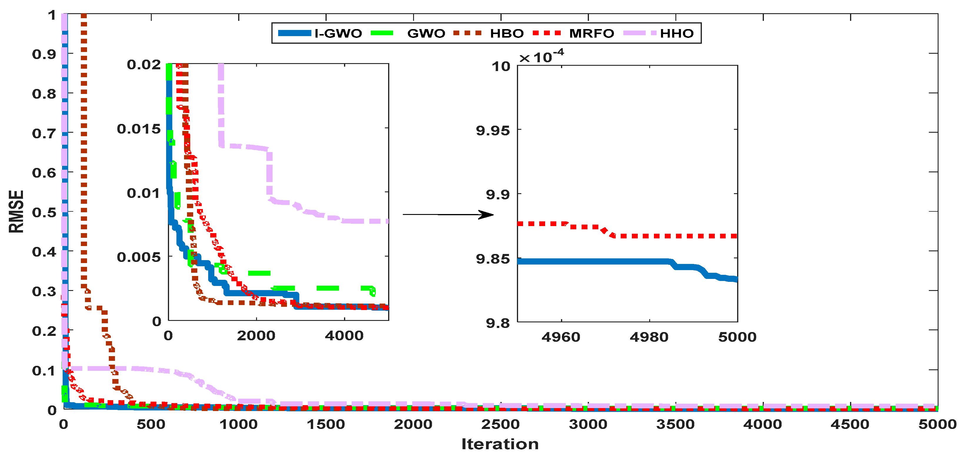
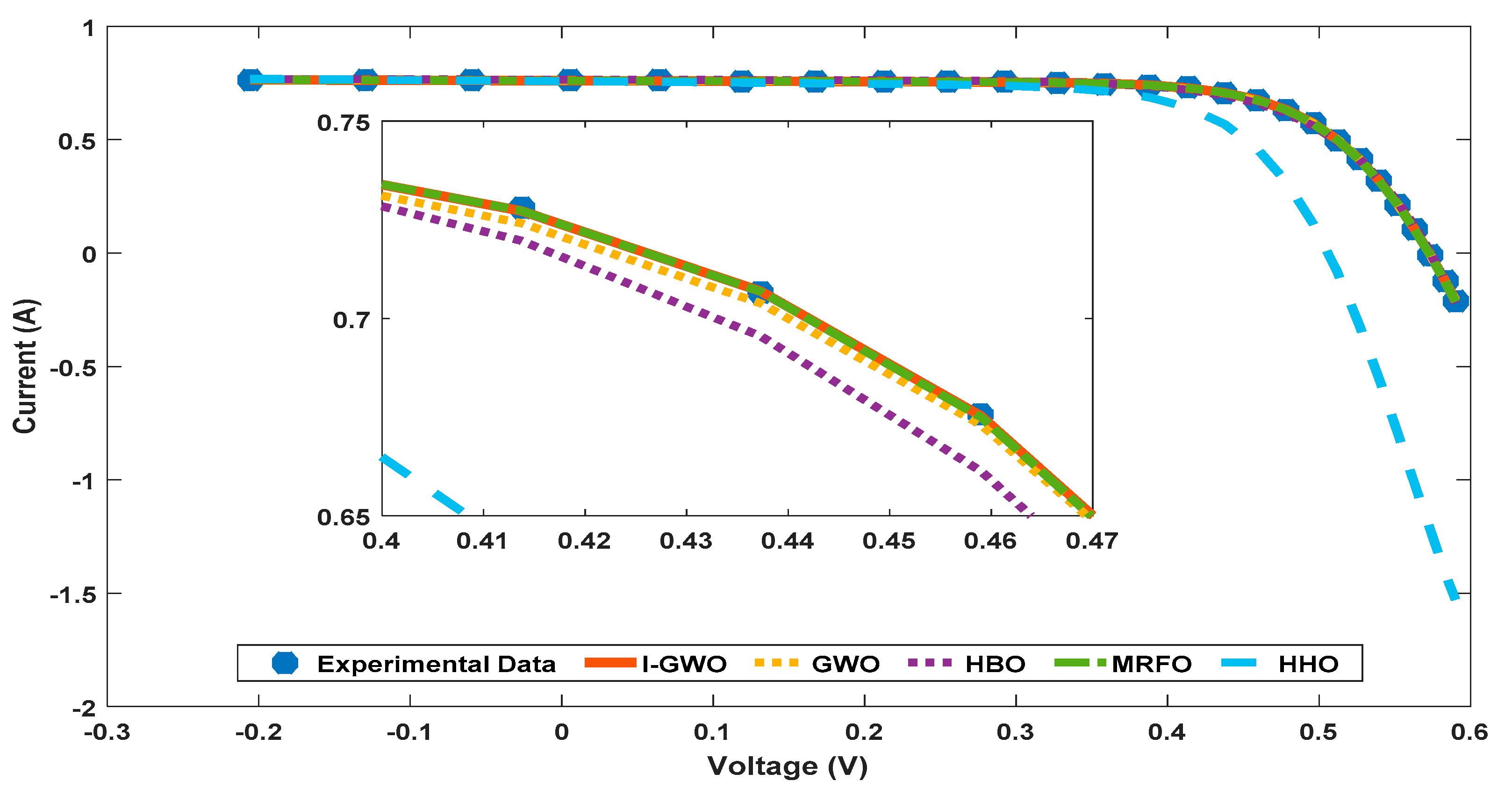
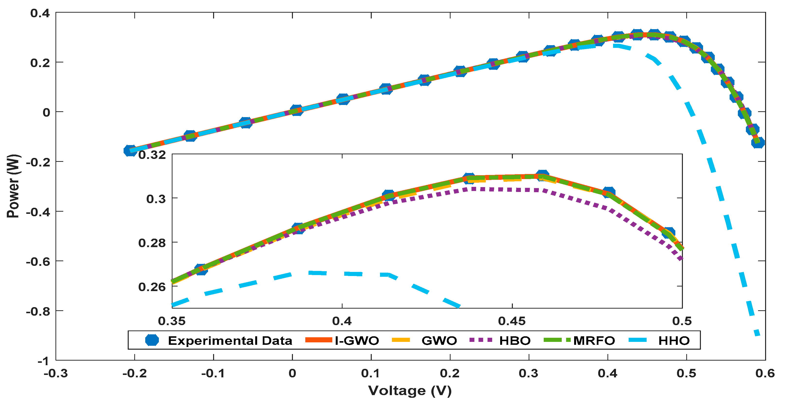
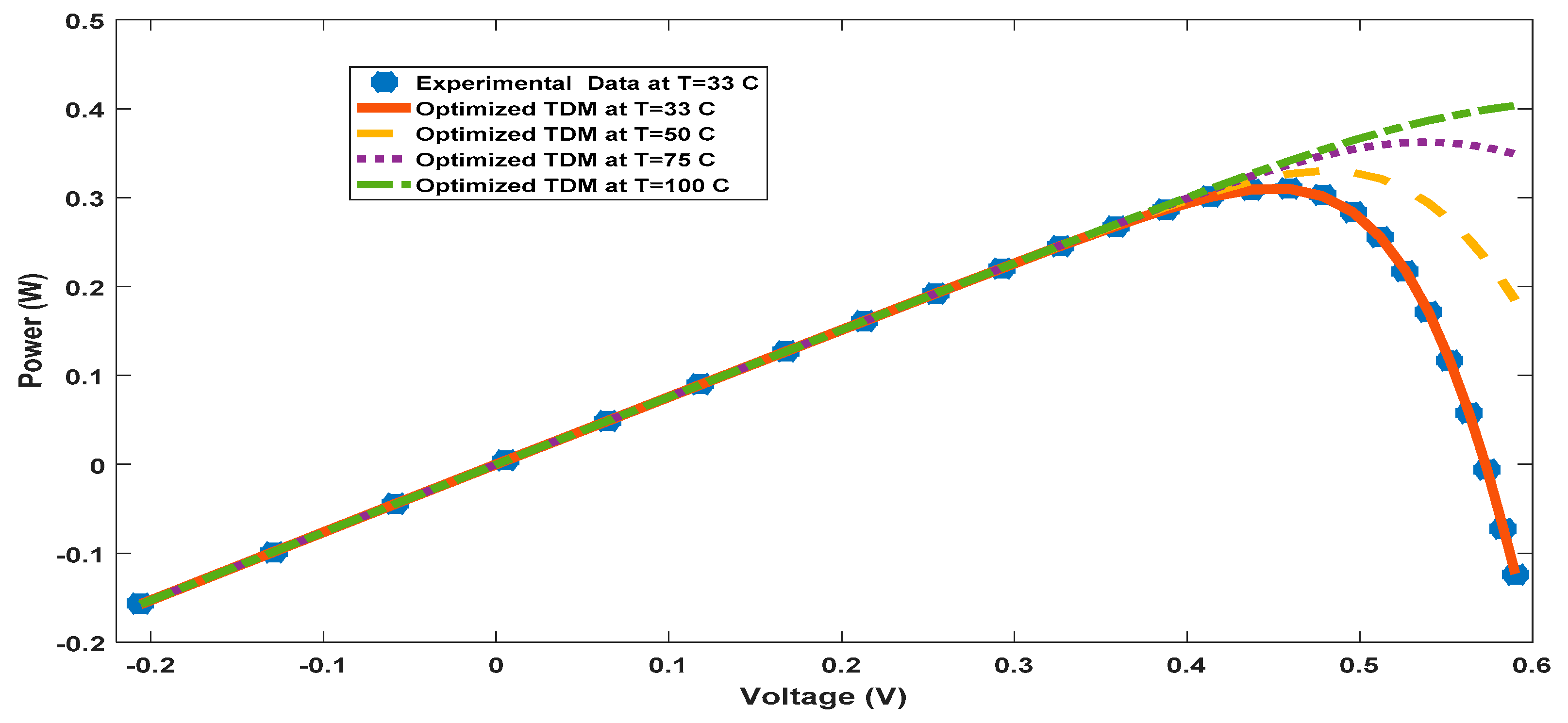
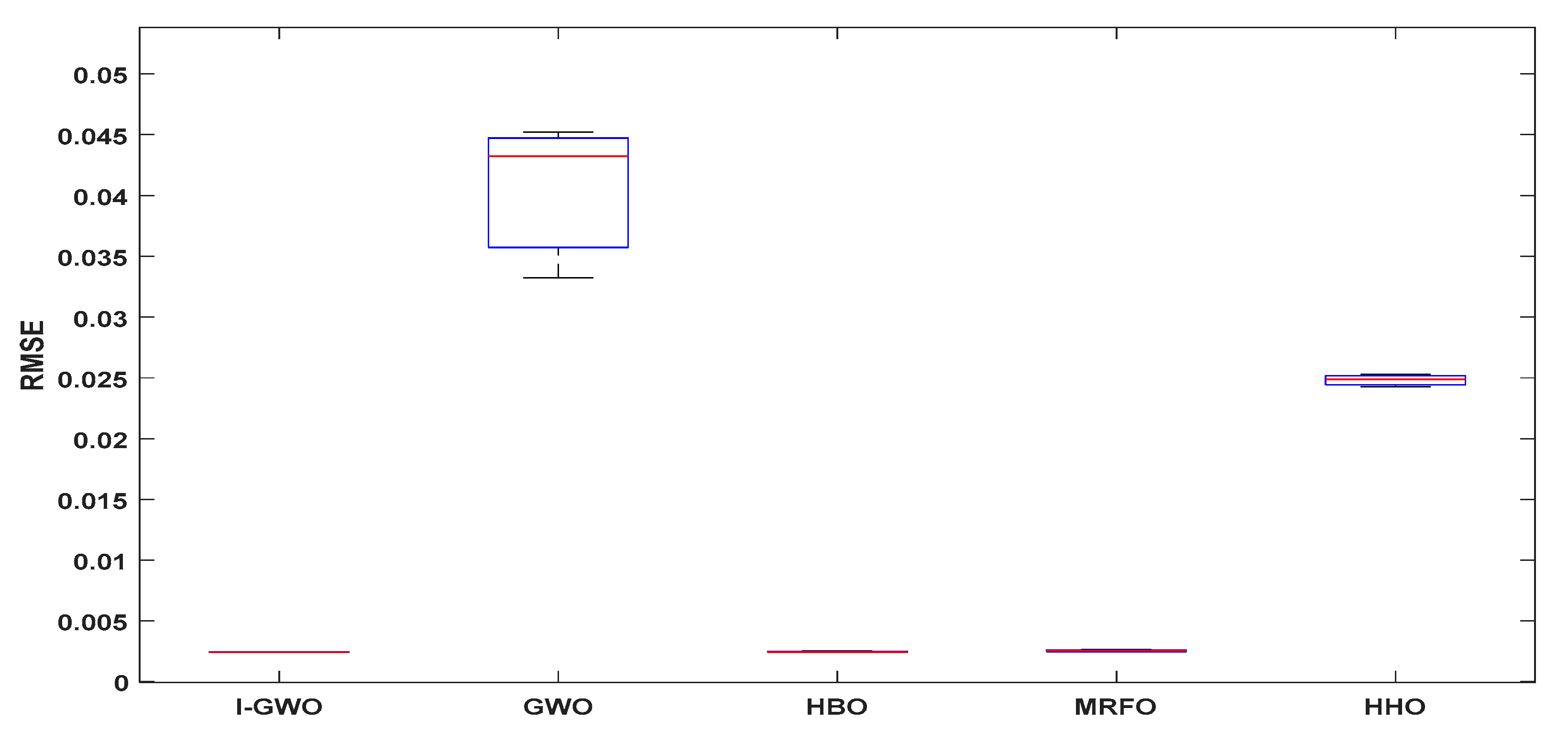
4. Results
4.1. Application #1:
4.2. Application #2:
5. Overall Discussion
6. Conclusions
Author Contributions
Funding
Institutional Review Board Statement
Informed Consent Statement
Data Availability Statement
Conflicts of Interest
Nomenclature
| Symbol | Description |
| TDM | Three Diode Model |
| RMSE | Root Mean Square Error |
| PV | Photo Voltaic |
| Ns | number of series solar cells |
| I | PV module output current |
| NP | number of parallel PV modules |
| V | Terminal voltage |
| XP(t) | Prey current position |
| Iph | Photo generated current source |
| X(t) | Gray wolf current position |
| ɳ1 | First Diode Ideality factor (Diffusion current components) |
| ɳ2 | Second Diode Ideality Factor (Recombination current components) |
| ɳ3 | Third diode Ideality Factor(Leakage current components) |
| Rsh | Equivalent Shunt resistance for current leakage resistance across the P-N junction of solar cell |
| Rs | Equivalent Series resistance for semiconductor material at neutral regions |
| K | =1.380 × 10⁻²³(J/Ko) Boltzmann constant |
| Is1 | First diode current |
| q | 1.602 × 10⁻¹⁹ (C) Coulombs. |
| Is2 | Second diode current |
| T (Ko) | Photo cell temperature (Kelvin) |
| Is3 | Third diode current |
| HBO | Heap-based optimizer |
| X(t) | Current position |
| X(t+1) | Position in next iteration |
| GWO | Grey Wolf Optimizer |
| I-GWO | Improved Grey Wolf Optimizer |
| HHO | Harries Hawk optimization |
| MRFO | Manta Ray Foraging Optimization |
References
- Humada, A.M.; Darweesh, K.G.M.; Kamil, M.; Samen, F.M.; Naseer, K.K.; Tahseen, A.T.; Omar, I.A.; Saad, M. Modeling of PV system and parameter extraction based on experimental data: Review and investigation. Sol. Energy 2020, 199, 742–760. [Google Scholar] [CrossRef]
- Gielen, D.; Boshell, F.; Saygin, D.; Bazilian, M.D.; Wagner, N.; Gorini, R. The role of renewable energy in the global energy transformation. Energy Strategy Rev. 2019, 24, 38–50. [Google Scholar] [CrossRef]
- Araújo, K.; Boucher, J.L.; Aphale, O. A clean energy assessment of early adopters in electric vehicle and solar photovoltaic technology: Geospatial, political and socio-demographic trends in New York. J. Clean. Prod. 2019, 216, 99–116. [Google Scholar] [CrossRef]
- Choudhary, P.; Srivastava, R.K. Sustainability perspectives—A review for solar photovoltaic trends and growth opportunities. J. Clean. Prod. 2019, 227, 589–612. [Google Scholar] [CrossRef]
- Singh, S.N.; Prabhakar, T.; Sumit, T. Introduction to solar energy. In Fundamentals and Innovations in Solar Energy; Springer: Singapore, 2021; pp. 1–9. [Google Scholar]
- Piyush, G. Importance of Detailed Modeling of Loads/PV Systems Connected to Secondary of Distribution Transformers. Master’s Thesis, Electrical Engineering Faculty of the Virginia Polytechnic Institute and State University, Blacksburg, VA, USA, 2017. [Google Scholar]
- Halabi, M.A.; Al-Qattana, A.; Al-Otaibi, A. Application of solar energy in the oil industry—Current status and future prospects. Renew. Sustain. Energy Rev. 2015, 43, 296–314. [Google Scholar] [CrossRef]
- Mekhilef, S.; Faramarzi, S.Z.; Saidur, R.; Salam, Z. The application of solar technologies for sustainable development of agricultural sector. Renew. Sustain. Energy Rev. 2013, 18, 583–594. [Google Scholar] [CrossRef]
- Zhang, Y.; Sivakumar, M.; Yang, S.; Enever, K.; Ramezanianpour, M. Application of solar energy in water treatment processes: A review. Desalination 2018, 428, 116–145. [Google Scholar] [CrossRef] [Green Version]
- Sharma, A.; Sharma, A.; Averbukh, M.; Jately, V.; Azzopardi, B. An effective method for parameter estimation of a solar cell. Electronics 2021, 10, 312. [Google Scholar] [CrossRef]
- Rodrigues, E.M.G.; Melicio, R.; Mendes, V.M.F.; Catalao, J.P. Simulation of a solar cell considering single-diode equivalent circuit model. RE&PQJ 2011. [Google Scholar] [CrossRef]
- Ma, J.; Man, K.L.; Ting, T.O.; Zhang, N.; Guan, S.U.; Wong, P.W. Wong approximate single-diode photovoltaic model for efficient I-V characteristics estimation. Sci. World J. 2013, 2013, 230471. [Google Scholar] [CrossRef] [PubMed] [Green Version]
- Sabadus, A.; Mihailetchi, V.; Paulescu, M. Parameters extraction for the one-diode model of a solar cell. In AIP Conference Proceedings; AIP Publishing LLC: Melville, NY, USA, 2017; p. 40005. [Google Scholar]
- Tamrakar, V.; Gupta, S.C.; Sawle, Y. Single-diode Pv cell modeling and study of characteristics of single and two-diode equivalent circuit. Electr. Electron. Eng. Int. J. 2015, 4, 12. [Google Scholar] [CrossRef]
- Tamrakar, V.; Gupta, S.C.; Sawle, Y. Single-diode and two-diode Pv cell modeling using matlab for studying characteristics of solar cell under varying conditions. Electr. Comput. Eng. Int. J. 2015, 4, 67–77. [Google Scholar] [CrossRef]
- Sulyok, G.; Summhammer, J. Extraction of a photovoltaic cell’s double-diode model parameters from data sheet values. Energy Sci. Eng. 2018, 6, 424–436. [Google Scholar] [CrossRef] [Green Version]
- Tanvir, A.; Sobhan, S.; Nayan, M.F. Comparative analysis between single diode and double diode model of PV cell: Concentrate different parameters effect on its efficiency. J. Power Energy Eng. 2016, 4, 31–46. [Google Scholar]
- Soliman, M.A.; Al-Durra, A.; Hasanien, H.M. Electrical parameters identification of three-diode photovoltaic model based on equilibrium optimizer algorithm. IEEE Access 2021, 9, 41891–41901. [Google Scholar] [CrossRef]
- Wang, R. Parameter identification of photovoltaic cell model based on enhanced particle swarm optimization. Sustainability 2021, 13, 840. [Google Scholar] [CrossRef]
- Khanna, V.; Das, B.K.; Bisht, D.; Singh, P.K. A three diode model for industrial solar cells and estimation of solar cell parameters using PSO algorithm. Renew. Energy 2015, 78, 105–113. [Google Scholar] [CrossRef]
- El-Hameed, M.A.; Elkholy, M.M.; El-Fergany, A.A. Three-diode model for characterization of industrial solar generating units using Manta-rays foraging optimizer: Analysis and validations. Energy Convers. Manag. 2020, 219, 113048. [Google Scholar] [CrossRef]
- Harrag, A.; Daili, Y. Three-diode PV model parameters extraction using PSO algorithm. Rev. Energ. Renouvelables 2019, 22, 85–91. [Google Scholar]
- Shekoofa, O.; Wang, J. Multi-diode modeling of multi-junction solar cells In Proceedings of the 23rd Iranian Conference on Electrical Engineering, Tehran, Iran, 10–14 May 2015.
- Ukoima, K.N.; Ekwe, O. A three-diode model and simulation of photovoltaic (Pv) cells. J. Eng. Technol. 2019, 5, 108–116. [Google Scholar]
- Bayoumi, A.S.; El-Sehiemy, R.A.; Mahmoud, K.; Lehtonen, M.; Darwish, M.M. Assessment of an improved three-diode against modified two-diode patterns of MCS solar cells associated with soft parameter estimation paradigms. Appl. Sci. 2021, 11, 1055. [Google Scholar] [CrossRef]
- Mehdi, O.; Mohamed, S.M.; Djalel, D.O. Comprehensive three-diode model of photovoltaic array with partial shading capability. Int. J. Power Energy Convers. 2018, 9, 159–173. [Google Scholar]
- Saha, C.; Agbu, N.; Jinks, R.; Huda, M.N. Review article of the solar PV parameters estimation using evolutionary algorithms. MOJ Sol. Photoenergy Syst. 2018, 2, 63–75. [Google Scholar]
- Qais, M.H.; Hasanien, H.M.; Alghuwainem, S. Parameters extraction of three-diode photovoltaic model using computation and Harris Hawks optimization. Energy 2020, 195, 117040. [Google Scholar] [CrossRef]
- Abdel-Basset, M.; Mohamed, R.; Mirjalili, S.; Chakrabortty, R.K.; Ryan, M.J. Solar photovoltaic parameter estimation using an improved equilibrium optimizer. Sol. Energy 2020, 209, 694–708. [Google Scholar] [CrossRef]
- Sheng, H.; Li, C.; Wang, H.; Yan, Z.; Xiong, Y.; Cao, Z.; Kuang, Q. Parameters extraction of photovoltaic models using an improved moth-flame optimization. Energies 2019, 12, 3527. [Google Scholar] [CrossRef] [Green Version]
- Elazab, O.S.; Hasanien, H.M.; Alsaidan, I.; Abdelaziz, A.Y.; Muyeen, S.M. Parameter estimation of three diode photovoltaic model using grasshopper optimization algorithm. Energies 2020, 13, 497. [Google Scholar] [CrossRef] [Green Version]
- Saxena, A.; Sharma, A.; Shekhawat, S. Parameter extraction of solar cell using intelligent grey wolf optimizer. Evol. Intell. 2020. [Google Scholar] [CrossRef]
- Nadimi-Shahraki, M.H.; Taghian, S.; Mirjalili, S. An improved grey wolf optimizer for solving engineering problems. Expert Syst. Appl. 2021, 166, 113917. [Google Scholar] [CrossRef]
- Qais, M.H.; Hasanien, H.M.; Alghuwainem, S.; Nouh, A.S. Coyote optimization algorithm for parameters extraction of three-diode photovoltaic model of photovoltaic modules. Energy 2019, 187, 116001. [Google Scholar] [CrossRef]
- Qais, M.H.; Hasanien, H.M.; Alghuwainem, S. Identification of electrical parameters for three-diode photovoltaic model using analytical and sunflower optimization algorithm. Appl. Energy 2019, 250, 109–117. [Google Scholar] [CrossRef]
- Mohamed, A.; Reda, M.; Attia, E.; Mohamed, A.; Askar, S.S. Parameters identification of PV triple-diode model using improved generalized normal distribution algorithm. Mathematics. 2021, 9, 995. [Google Scholar]
- Allam, D.; Yousri, D.A.; Eteiba, M.B. Parameters extraction of the three diode model for the multi-crystalline solar cell/module using Moth-Flame Optimization Algorithm. Energy Convers. Manag. 2016, 123, 535–548. [Google Scholar] [CrossRef]
- Mirjalili, S.; Mirjalili, S.M.; Lewisa, A. Grey wolf optimizer. Adv. Eng. Softw. 2014, 69, 46–61. [Google Scholar] [CrossRef] [Green Version]
- Roy, R.G.; Ghoshal, D. Grey wolf optimization-based second order sliding mode control for inchworm robot. Robotica 2019, 38, 1–19. [Google Scholar] [CrossRef]
- Luo, K.; Zhao, O. A binary grey wolf optimizer for the multidimensional knapsack problem. Appl. Soft Comput. 2019, 83, 105645. [Google Scholar] [CrossRef]
- Pal, A.; Bahuguna, S. Grey wolf optimizer. Future Asp. Eng. Sci. Technol. 2018, 36, 379–382. [Google Scholar]
- Sharma, I.; Chahar, V.; Agri, S. A comprehensive survey on grey wolf optimization. Recent Pat. Comput. Sci. 2020, 13, 1–13. [Google Scholar] [CrossRef]
- Abdelghany, R.Y.; Kamel, S.; Ramadan, A.; Sultan, H.; Rahmann, C. Solar cell parameter estimation using school-based optimization algorithm. In Proceedings of the IEEE International Conference on Automation/XXIV Congress of the Chilean Association of Automatic Control, Santiago, Chile, 22–26 March 2021. [Google Scholar]
- Ramadan, A.; Kamel, S.; Korashy, A.; Yu, J. Photovoltaic cells parameter estimation using an enhanced teaching learning based optimization algorithm. Iran. J. Sci. Technol. 2019, 44, 767–779. [Google Scholar] [CrossRef]
- Ramadan, A.; Kamel, S.; Hussein, N.M.; Hassan, M.H. A new application of chaos game optimization algorithm for parameters extraction of three diode photovoltaic model. IEEE Access 2021, 9, 51582–51594. [Google Scholar] [CrossRef]
- Liao, Z.; Chen, Z.; Li, S. Parameters extraction of photovoltaic models using triple-phase teaching-learning-based optimization. IEEE Access 2019, 7, 77629–77641. [Google Scholar] [CrossRef]


| IGWO | GWO | HBO | MRFO | HHO | |
|---|---|---|---|---|---|
| Rs(Ω) | 0.0367 | 0.043821 | 0.040 | 0.03634 | 0.018333 |
| Rsh(Ω) | 54.888 | 59.64 | 59.997 | 53.9246 | 92.25011 |
| Iph(A) | 0.7607 | 0.7619 | 0.7608 | 0.76078 | 0.764769 |
| Isd1(A) | 2.27 × 10⁻⁷ | 1.38 × 10⁻¹⁰ | 6.97 × 10⁻⁷ | 2.67 × 10⁻⁸ | 3.82 × 10⁻⁶ |
| Isd2(A) | 3.14 × 10⁻⁷ | 2.51 × 10⁻¹⁰ | 1.00 × 10⁻¹⁰ | 1.54 × 10⁻⁸ | 2.71 × 10⁻⁶ |
| Isd3(A) | 2.34 × 10⁻⁷ | 4.07 × 10⁻⁶ | 1.59472 | 3.17 × 10⁻⁷ | 1.28 × 10⁻⁶ |
| N1 | 1.9256 | 1.6677 | 1.009 | 1.9076 | 1.882327 |
| N2 | 1.9600 | 1.0181 | 1.0082 | 1.8674 | 1.891646 |
| N3 | 1.4500 | 1.9182 | 1.3083 | 1.475 | 1.891677 |
| RMSE | 0.00098331 | 0.00191 | 0.001120 | 0.000986002 | 0.007721 |
| Algorithm | Parameter Setting | |
|---|---|---|
| I-GWO | r1 = rand() | r2 = rand() |
| GWO | r1 = rand() | r2 = rand() |
| HBO | degree = 3 | |
| MRFO | NP = 1000 | S = 2 |
| Minimum | Average | Maximum | STD | |
|---|---|---|---|---|
| I-GWO | 0.000983 | 0.000984 | 0.000985 | 6.60404 × 10⁻⁷ |
| GWO | 0.001298 | 0.00751 | 0.019319 | 0.010231343 |
| HBO | 0.00112 | 0.001606667 | 0.0024 | 0.000692917 |
| MRFO | 0.000986 | 0.000987 | 0.000989 | 1.25983 × 10⁻⁶ |
| HHO | 0.0077205 | 0.0117475 | 0.01917 | 0.006435824 |
| I-GWO | GWO | HBO | MRFO | HHO | |
|---|---|---|---|---|---|
| Rs(Ω) | 1.198683773 | 1.666138 | 1.199582 | 1.210609373 | 1.804672596 |
| Rsh(Ω) | 986.3365886 | 60 | 983.629 | 799.9841045 | 358.9956246 |
| Iph(A) | 1.030508846 | 1.153399 | 1.030447 | 1.032037975 | 1.025407497 |
| Isd1(A) | 1.25 × 10⁻⁶ | 1.48 × 10⁻¹⁰ | 3.48 × 10⁻⁷ | 6.20 × 10⁻⁸ | 6.07 × 10⁻¹⁰ |
| Isd2(A) | 7.77 × 10⁻⁷ | 1.83 × 10⁻¹⁰ | 1.00 × 10⁻¹⁰ | 1.97 × 10⁻⁶ | 1.24 × 10⁻⁹ |
| Isd3(A) | 1.54 × 10⁻⁶ | 2.35 × 10⁻¹⁰ | 3.19 × 10⁻⁶ | 1.09 × 10⁻⁶ | 4.89 × 10⁻¹⁰ |
| N1 | 49.2667226 | 28.09997 | 48.60267 | 48.2266307 | 29.89953654 |
| N2 | 48.38422661 | 28.13075 | 49.52947 | 48.08828143 | 33.55517196 |
| N3 | 48.25593375 | 46.03489 | 48.56558 | 48.09442382 | 29.53540241 |
| RMSE | 0.0024276291 | 0.03323 | 0.0024281 | 0.0024609 | 0.024273 |
| Minimum | Average | Maximum | STD | |
|---|---|---|---|---|
| I-GWO | 0.002427629 | 0.002432 | 0.002438 | 5.26003 × 10⁻⁶ |
| GWO | 0.03323 | 0.040563 | 0.04523 | 0.006429101 |
| HBO | 0.0024281 | 0.002465 | 0.002528 | 5.50757 × 10⁻⁵ |
| MRFO | 0.0024609 | 0.002554 | 0.002641 | 9.0185 × 10⁻⁵ |
| HHO | 0.024273 | 0.024806 | 0.025273 | 0.000503322 |
Publisher’s Note: MDPI stays neutral with regard to jurisdictional claims in published maps and institutional affiliations. |
© 2021 by the authors. Licensee MDPI, Basel, Switzerland. This article is an open access article distributed under the terms and conditions of the Creative Commons Attribution (CC BY) license (https://creativecommons.org/licenses/by/4.0/).
Share and Cite
Ramadan, A.-E.; Kamel, S.; Khurshaid, T.; Oh, S.-R.; Rhee, S.-B. Parameter Extraction of Three Diode Solar Photovoltaic Model Using Improved Grey Wolf Optimizer. Sustainability 2021, 13, 6963. https://0-doi-org.brum.beds.ac.uk/10.3390/su13126963
Ramadan A-E, Kamel S, Khurshaid T, Oh S-R, Rhee S-B. Parameter Extraction of Three Diode Solar Photovoltaic Model Using Improved Grey Wolf Optimizer. Sustainability. 2021; 13(12):6963. https://0-doi-org.brum.beds.ac.uk/10.3390/su13126963
Chicago/Turabian StyleRamadan, Abd-ElHady, Salah Kamel, Tahir Khurshaid, Seung-Ryle Oh, and Sang-Bong Rhee. 2021. "Parameter Extraction of Three Diode Solar Photovoltaic Model Using Improved Grey Wolf Optimizer" Sustainability 13, no. 12: 6963. https://0-doi-org.brum.beds.ac.uk/10.3390/su13126963