A Continuous Transportation Network Design Problem with the Consideration of Road Congestion Charging

Abstract

This paper proposes a biobjective continuous transportation network design problem concerning road congestion charging with the consideration of speed limit. The efficiency of the traffic network and the reduction of pollution in the network environment are improved by designing a reasonable road capacity enhancement and speed limit strategy. A biobjective bilevel programming model is developed to formulate the proposed network design problem. The first target of the upper problem is the optimization of road charging efficiency, and the other target is the total cost of vehicle emissions; these objectives are required to devise the optimal road capacity enhancement scheme, speed limiting schemes for different time periods, and the road pricing scheme. The lower-level problem involving travellers’ route choice behaviours uses stochastic user equilibrium (SUE) theory. Based on the nondominated sorting genetic algorithm, which is applied to solve the bilevel programming model, a numerical example is developed to illustrate the effectiveness of the proposed model and algorithm. The results show that the implementation of congestion charging measures on the congested road sections would help to alleviate road congestion in the transportation network, effectively save transportation infrastructure investment and limited urban land resources, increase fiscal revenue, and open up new sources of funds for urban infrastructure construction.

1. Introduction

The conventional continuous network design problem (CNDP) aims to optimally balance the transportation and investment costs of a network subject to traffic congestion. Since its first formulation as a bilevel programming problem by Abdulaal and LeBlanc [1], CNDP has become one of the most difficult yet challenging problems in the transportation research field [2,3]. In the past two decades, many scholars have studied the solution under constraint adjustment. This research mainly focuses on the speed limit in the continuous traffic network design problem while adding the control strategy of road congestion charging. In this way, the operating efficiency of the transportation network will be improved, and the pollution discharge to the environment will be reduced.

CNDP has been a subject of substantial research, and a number of solution methods have been proposed to find a local optimum solution [4]. Meng et al. [5] presented the augmented Lagrangian method to solve CNDPs, especially for large networks. Xu et al. [6] proposed the use of simulated annealing (SA) and the GA to achieve good results when solving CNDPs. Unlike Xu et al. [6], Mathew and Sarma [7] reported that the GA model is more efficient for CNDPs than the other compared algorithms that were available in the literature. Gao et al. [8] and Wang and Lo [9] tried to solve a CNDP by considering it as a single-level problem. Recently, Li et al. [10] and Baskan [11,12] also attempted to solve the bilevel formulation of a CNDP using three powerful heuristics for solving CNDPs. However, Karoonsoontawong and Waller [13], Yinghui et al. [14], and Lu et al. [15] all tried to use heuristic methods to solve NDPs and finally found that the genetic algorithm (GA) produced better results than those of other algorithms in terms of some performance indicators. Therefore, this paper further adopts the genetic algorithm based on the nondominated sorting.

The first study of CNDPs based on SUE traffic assignment was presented by Davis [16], in which two different methods considering the effects of stochastic user equilibria were proposed for solving CNDPs, and these methods were applied to several test networks. Liu and Wang [17] and Du and Wang [18] proposed different methods for achieving the global solution of a CNDP by considering the SUE assumption. Similar to this study, Long et al. [19] developed a bilevel programming model to solve the turning restriction design problem with SUE. A recent study on the multimodal network design problem (MNDP, a combination of a CNDP and DNDP) was conducted by Gallo et al. [20], in which an SUE traffic assignment was considered at the lower level of the problem, while the total travel time in the network was minimized at the upper level via the scatter search method. As opposed to these articles, the lower-level problem of this research compares the stochastic user equilibrium (SUE) traffic assignment and the user equilibrium (UE) traffic assignment.

Speed limits are an effective means of traffic control, and their implementation can effectively improve traffic efficiency, the traffic environment, and traffic safety [21]. In recent years, many scholars have studied speed limits from the perspective of entire road network systems, including the impact of a speed limit on travel behaviour [22,23], dynamic speed limits [24], and the combinations of speed limits and other traffic policies [25,26]. Travel time is regarded as the principle of passenger route selection, which realizes the user equilibrium of speed limit and reliability [27]. Moreover, the travel time cost and congestion risk are perceived in advance, and the speed limit scheme composed of a specific network is realized [28]. The above speed limit research on the improvement of traffic network performance has important reference value for the proposal and integration of a speed limit strategy in this paper.

Congestion pricing is one of the most widely contemplated methods to manage traffic congestion by charging fees for the use of roads: a higher fee where and when it is congested, and a lower one where and when it is not [29,30]. At present, there have been many studies on congestion pricing, especially in urban network pricing. In the past two years, cumulative prospect theory (CPT) has been used to quantify the travel satisfaction of tourists, and the perceived service level of tourists has also been taken into account, so as to reduce the travel demand during peak hours based on regional congestion pricing [31]. The economic scale of the hub and network is also taken into account. The optimal design of hub and network space is realized by taking economic scale as the concave linear function and the congestion degree as the convex linear function [32]. In addition, a two-stage distributed solution is proposed to solve the optimal time congestion pricing problem in large-scale networks, so as to realize the whole network capture of the congestion charging area effect [33]. Therefore, it can be seen from recent studies that congestion pricing is still used as a separate efficiency improvement strategy in the problem of network smoothness, and it does not achieve the integration of congestion pricing and speed limit-related strategies. In this paper, we propose an efficiency improvement method integrating congestion charging and speed limit, in an attempt to further solve the problems of network congestion and operation efficiency in the new method integration.

Additionally, it is necessary to use both speed limit and congestion charging to improve efficiency and solve the CNDP problem. The influence of these two measures on the objective function can be observed more comprehensively, so as to better improve the efficiency of the network and the emission of pollutants.

Based on the traditional network design problem, this paper proposes a dual-objective transportation network design problem. The contribution and innovation of this article are as follows:

(1)

Different from previous studies, this paper simultaneously considers the optimization of speed limit strategy and congestion pricing strategy under different traffic demand periods. Instead of the independent CNDP solutions, the speed limit strategy and congestion charging strategy are not only combined in this study, but they are also able to play their advantages under different needs, which could better solve the CNDP problem and provide a new idea for CNDP by the combination of multiple strategies.

(2)

Secondly, this paper compares the differences between the two allocation models when solving the lower-level problem. In CNDP, the underlying problem is generally defined as UE or SUE traffic allocation [19,20]. This paper compares the results of traffic allocation based on these two methods and finds that the traffic assignment method based on SUE avoids the large sensitivity problem. Although the impedance based on SUE is larger than that based on UE, the traffic flow is more even when using SUE.

(3)

Moreover, this research designs an NSGA-II algorithm to solve the biobjective and bilevel programming model. The introduction of the NSGA-II algorithm realizes an innovative solution of the CNDP problem and solves the complex calculation process of CNDP optimization. For the method itself, it not only maintains the diversity and distribution uniformity of the population in the solution process, but it also ensures that the best individuals at all levels will not be lost. Finally, a numerical example is provided to verify the effectiveness and practicability of the model and algorithm.

The rest of the paper is presented as follows. The biobjective bilevel programming model for solving the CNDP described above is given in Section 2. A GA based on the nondominated sorting method is presented in the subsequent section. In Section 4, the Nguyen-Dupuis network is used to verify the effectiveness of the proposed model and algorithm. Finally, conclusions are given in Section 5.

2. Biobjective Bilevel Programming Model

Congestion pricing refers to charging vehicles at specific times and sections of a road to change the travel times, modes, and routes of travellers; this scheme plays a regulatory role in terms of the volumes (in time and space) of traffic trips to alleviate traffic congestion.

$W$	set of OD pairs, where $w\in W$ denotes an OD pair
$M$	set of different times of the day, $m\in M$
$P_w$	set of paths between an OD pair, $p\in P_w$
$A_0$	a collection of sections with their speed limits
$L_a$	length of section a
$d_w^m$	travel demand between OD pair $w\in W$ during $m\in M$
$f_{r,w}^m$	the r-th path flow between OD pair $w\in W$ during $m\in M$
$t_a(v_a^m)$	time impedance function of section a during $m\in M$
$v_a^m$	traffic flow of section a during $m\in M$
$t_a^0$	free-flow travel time within section a
$y_a$	increased capacity of section a
$s_a$	average driving speed within section a
$s_a^C$	lowest speed limit of section a
${\overline{s}}_a$	speed limit value of section a
$C_a$	maximum practical capacity of section a
${\delta }_{a,k}^{}$	the correlation factor between section a and path k

2.1. Stochastic User Equilibrium Assignment Problem

In the case where speed limits exist on urban road sections, the link impedance function of a section with a speed limit will differ according to the changes in the traffic volume within that road section. Under speed limit conditions, the section impedance function can be expressed as

$$t_a\left(v_a\right)=\{\begin{array}{c}{\overline{t}}_a\hspace{0.17em}\hspace{0.17em}\hspace{0.17em}\hspace{0.17em}\hspace{0.17em}\hspace{0.17em}\hspace{0.17em}\hspace{0.17em}\hspace{0.17em}\hspace{0.17em}\hspace{0.17em}0\le v_a\le {\overline{v}}_a\\ \hspace{0.17em}\hspace{0.17em}{\tilde{t}}_a\left(v_a\right)\hspace{0.17em}\hspace{0.17em}\hspace{0.17em}\hspace{0.17em}\hspace{0.17em}\hspace{0.17em}{\overline{v}}_a<v_a\le C_a\end{array}\hspace{0.17em}$$

(1)

where ${\overline{v}}_a$ represents the traffic flow of road section $a$ under the speed limit, and ${\overline{t}}_a\hspace{0.17em}$ represents the travel time when road section $a$ has a speed limit. $\hspace{0.17em}{\tilde{t}}_a\left(v_a\right)$ represents the travel time function when there is no speed limit imposed on the road section, and ${\overline{t}}_a={\tilde{t}}_a\left({\overline{v}}_a\right)$. Under the speed limit ${\overline{s}}_a$, ${\overline{t}}_a=L_a/{\overline{s}}_a$ and ${\overline{v}}_a={\tilde{t}}_a{}^{-1}\left(L_a/{\overline{s}}_a\right)$, where ${\tilde{t}}_a{}^{-1}(\cdot )$ is the inverse of the impedance function for road section $a$ under the condition of infinite speed.

The model for the lower-layer problem uses an SUE model to describe travellers’ path selection behaviour. First, we separately consider the generalized road travel time function under congestion charging measures. A congestion charge $g_a$ is imposed on section $\hspace{0.17em}a\in A^{+}$, and no congestion charges are imposed on the rest of the sections. Then, considering the congestion charging condition, the section impedance function is as follows:

$$t_a\left(v_a\right)=\{\begin{array}{c}{\tilde{t}}_a\left(v_a\right)+g_a\hspace{0.17em}\hspace{0.17em}\hspace{0.17em}\hspace{0.17em}\hspace{0.17em}\hspace{0.17em}\hspace{0.17em}\hspace{0.17em}\hspace{0.17em}\hspace{0.17em}a\in A^{+}\\ \hspace{0.17em}\hspace{0.17em}{\tilde{t}}_a\left(v_a\right)\hspace{0.17em}\hspace{0.17em}\hspace{0.17em}\hspace{0.17em}\hspace{0.17em}\hspace{0.17em}\hspace{0.17em}\hspace{0.17em}\hspace{0.17em}\hspace{0.17em}\hspace{0.17em}\hspace{0.17em}\hspace{0.17em}\hspace{0.17em}\hspace{0.17em}\hspace{0.17em}a\in A^{+C}\end{array}\hspace{0.17em}$$

(2)

where $A^{+}$ refers to a road section with crowded tolls, and $A^{+C}$ denotes a section without congestion pricing.

When we consider both congestion pricing and speed limits, the section impedance function is as follows:

$$t_a\left(v_a\right)=\{\begin{array}{c}\begin{array}{l}{\overline{t}}_a+\hspace{0.17em}{g}_a\hspace{0.17em}\hspace{0.17em}\hspace{0.17em}\hspace{0.17em}\hspace{0.17em}\hspace{0.17em}\hspace{0.17em}\hspace{0.17em}\hspace{0.17em}\hspace{0.17em}\hspace{0.17em}\hspace{0.17em}0\le v_a\le {\overline{v}}_a,a\in A^{+}\\ {\tilde{t}}_a\left(v_a\right)+g_a\hspace{0.17em}\hspace{0.17em}\hspace{0.17em}\hspace{0.17em}\hspace{0.17em}\hspace{0.17em}{\overline{v}}_a<v_a\le C_a,a\in A^{+}\end{array}\\ \begin{array}{l}\hspace{0.17em}{\overline{t}}_a\hspace{0.17em}\hspace{0.17em}\hspace{0.17em}\hspace{0.17em}\hspace{0.17em}\hspace{0.17em}\hspace{0.17em}\hspace{0.17em}\hspace{0.17em}\hspace{0.17em}\hspace{0.17em}\hspace{0.17em}\hspace{0.17em}\hspace{0.17em}\hspace{0.17em}\hspace{0.17em}\hspace{0.17em}\hspace{0.17em}0\le v_a\le {\overline{v}}_a,a\in A^{+C}\\ {\tilde{t}}_a\left(v_a\right)\hspace{0.17em}\hspace{0.17em}\hspace{0.17em}\hspace{0.17em}\hspace{0.17em}\hspace{0.17em}\hspace{0.17em}\hspace{0.17em}\hspace{0.17em}\hspace{0.17em}\hspace{0.17em}\hspace{0.17em}\hspace{0.17em}{\overline{v}}_a<v_a\le C_a,a\in A^{+C}\end{array}\end{array}\hspace{0.17em}$$

(3)

Considering the widening of road capacity, we adopt the following impedance function:

$${\tilde{t}}_a\left(v_a,y_a\right)=\alpha +\beta {(v_a/(C_a+y_a))}^4$$

(4)

where $\alpha$ and $\beta$ are the retardation coefficients. In the traffic flow assignment program of the United States Federal Highway Administration, the values of $\alpha$ and $\beta$ are $\alpha =0.15$ and $\beta =4$, respectively. In a practical application process, these parameters can also be adjusted through regression analysis. Equation (3) shows that the section impedance $t_a\left(v_a\right)$ is also a function of the speed limit ${\overline{s}}_a$, congestion charge $g_a$, and widening capacity $y_a$.

Similar to the general random user-balanced distribution model, the selection probability $f_k^{rs}$ of path k can be calculated by the cross-nested logit model. The flow of path k in the OD matrix (w) during period m can be expressed as follows:

$$f_k^{m,w}=d_w^m{P}_k^{m,w}$$

(5)

where $P_k^{m,w}$ represents the selection probability of path k in the OD matrix (w).

According to the relationships between sections and paths, the flow of section a in period m can be obtained:

$$v_a^m={\displaystyle \sum _w{\displaystyle \sum _k{f}_k^{m,w}{\delta }_{a,k}^{}}}={\displaystyle \sum _w{\displaystyle \sum _k{d}_w^m{P}_k^{m,w}{\delta }_{a,k}^{}}}$$

(6)

According to Yang et al. [25], the section balance flow of SUE traffic allocation based on the logit model can be obtained through the above flow conservation relationship.

2.2. Upper Biobjective Optimization Problem

From the perspective of traffic management, the upper level of the network design problem can improve the operating efficiency of the traffic network and reduce the total vehicle exhaust emissions by improving the traffic capacity of each section and setting reasonable speed limits for the section during different periods. Therefore, the upper-level problem can be described as a biobjective optimization problem.

(1)

System Travel Costs

Time is the most important factor in many traffic impedances. In some traffic networks, the travel time and distance of a section can be regarded as an approximate proportional relationship, and they have nothing to do with the traffic flow in the section, such as in an urban rail transit network. However, in some traffic networks, the driving time of a section is not necessarily proportional to the driving distance but is related to the traffic flow of a section in the traffic network, such as an urban road network. The function form of the total system travel cost C is as follows:

$$C={\displaystyle \sum _{a\in A}{v}_a\cdot t_a\left(v_a\right)}$$

(7)

(2)

Investment Expenses

In urban road network design, the expansion of the traffic capacities of existing sections is considered. There are generally two forms of capacity expansion: one is discrete, that is, to expand the number of lanes in a section. The other is continuous, which involves expanding the existing traffic capacity of a section. The expansion cost is usually converted into the travel cost of the system through a matching coefficient, and its functional form is as follows:

$$E=\varphi {\displaystyle \sum _a{G}_a(y_a)}$$

(8)

$$y_a\ge 0,\forall a\in A$$

(9)

where $\varphi$ represents the investment expense matching coefficient, namely for matching the investment expense to the travel time of the system. Equation (9) indicates that there is a nonnegative constraint on the expansion of the section capacity. When $y_a$ is an integer, it represents the number of expanded lanes; otherwise, it is merely the expansion of existing capacity.

(3)

Vehicle Emission Cost

It is assumed that the exhaust emissions of a given road section are a function of the average vehicle speed and have the following functional form:

$${\phi }_a^n\left(v_a^m\right)=\frac{A_n\exp \left\{B_n{s}_a^m\right\}}{C_n{s}_a^m}$$

(10)

where $A_n$, $B_n$, and $C_n$ are the coefficients of the exhaust emission function of pollutant n, and $s_a^m$ is the average driving speed in section $a$ during period m. Therefore,

$$s_a^m=\frac{L_a}{t_a(v_a^m)}$$

(11)

The total exhaust emissions of the whole network can be calculated as follows:

$$E=\hspace{0.17em}{\displaystyle \sum _{m\in M}{\displaystyle \sum _{n\in N}{\displaystyle \sum _{a\in A}{\eta }_n\cdot v_a^m\cdot {\phi }_a^n(v_a^m)\cdot t_a(v_a^m)}}}$$

(12)

where ${\eta }_n$ is the unit emission cost of pollutant $n$, and ${\phi }_a^n\left(v_a^m\right)$ is the tail gas emission factor of pollutant n when the flow rate of road section $a$ is $v_a$ during period m.

(4)

Biobjective Optimization Model

The upper-layer problem aims at reducing the total impedance of the system and the total exhaust emissions of the traffic network to improve the performance of the network. Considering different traffic demand levels in different periods, the upper-level biobjective optimization problem can be expressed as follows:

$$\min \hspace{0.17em}\hspace{0.17em}\hspace{0.17em}{Z}_1\hspace{0.17em}=\hspace{0.17em}{\displaystyle \sum _{m\in M}{\displaystyle \sum _{a\in A}{t}_a\left(v_a^m\right)\hspace{0.17em}}}{v}_a^m+\theta {\displaystyle \sum _a{G}_a(y_a)}$$

(13)

$$\min \hspace{0.17em}\hspace{0.17em}\hspace{0.17em}{Z}_2\hspace{0.17em}=\hspace{0.17em}{\displaystyle \sum _{m\in M}{\displaystyle \sum _{n\in N}{\displaystyle \sum _{a\in A}{\eta }_n\cdot v_a^m\cdot {\phi }_a^n\left(v_a^m\right)\cdot t_a(v_a^m)}}}$$

(14)

$$\mathrm{s}.\mathrm{t}.\hspace{0.17em}0\le y_a\le {\overline{y}}_a\hspace{0.17em}\hspace{0.17em}\hspace{0.17em}\forall a\in A$$

(15)

$$s_a^m\ge \hspace{0.17em}{s}_a^C\hspace{0.17em}\hspace{0.17em}\hspace{0.17em}\hspace{0.17em}\hspace{0.17em}\hspace{0.17em}\hspace{0.17em}\hspace{0.17em}\forall a\in A_0,\forall m\in M$$

(16)

Objective function (13) minimizes the total impedance of the system and the investment matching cost, objective function (14) minimizes the total network exhaust emissions, and constraint conditions (15) and (16) are the section capacity expansion constraints and section speed limit conditions, respectively. The section flow $v_a^m$ is obtained by solving the balance distribution problem for lower users.

Considering the speed limit, the traffic management method of road congestion pricing is also added. Therefore, in addition to the total network impedance and the investment matching cost of the upper problem, the road pricing benefit is also considered. When congestion pricing is increased, considering different traffic demand levels during different periods, the upper biobjective optimization problem can be expressed as follows:

$$\min \hspace{0.17em}\hspace{0.17em}\hspace{0.17em}{Z}_1\hspace{0.17em}=\hspace{0.17em}{\displaystyle \sum _{m\in M}{\displaystyle \sum _{a\in A}{t}_a\left(v_a^m\right)\hspace{0.17em}}}{v}_a^m+\theta {\displaystyle \sum _a{G}_a(y_a)}-\tau \cdot {\displaystyle \sum _a{g}_a\cdot v_a}$$

(17)

$$\min \hspace{0.17em}\hspace{0.17em}\hspace{0.17em}{Z}_2\hspace{0.17em}=\hspace{0.17em}{\displaystyle \sum _{m\in M}{\displaystyle \sum _{n\in N}{\displaystyle \sum _{a\in A}{\eta }_n\cdot v_a^m\cdot {\phi }_a^n\left(v_a^m\right)\cdot t_a(v_a^m)}}}$$

(18)

$$\mathrm{s}.\mathrm{t}.0\le y_a\le {\overline{y}}_a\hspace{0.17em}\hspace{0.17em}\hspace{0.17em}\forall a\in A$$

(19)

$$s_a^m\ge \hspace{0.17em}{s}_a^C\hspace{0.17em}\hspace{0.17em}\hspace{0.17em}\hspace{0.17em}\hspace{0.17em}\hspace{0.17em}\hspace{0.17em}\hspace{0.17em}\forall a\in A_0,\forall m\in M$$

(20)

Objective function (17) is used to minimize the system total impedance (including the travel cost, investment cost, and congestion charging benefit), and objective function (18) is used to minimize the overall emissions of the network. Constraint conditions (19) and (20) are the restriction conditions with respect to road section capacity expansion, road section speed limits, and road congestion charging, respectively. The section flow $v_a^m$ is obtained by solving the equilibrium allocation problem of lower random users.

3. Solution Algorithm

3.1. Solution of the Lower Level Problem

The lower-layer model adopts the SUE allocation model. For lower-layer network users with a given road section capacity and road section speed limit, their path selection behaviour conforms to the SUE criterion. In general, the method of successive averages (MSA) is mostly used to solve the lower-level stochastic user balance problem. In the MSA, a deterministic step size method is used, which causes the algorithm to converge slowly because the step size is typically too large or too small. The self-adaption of the weighted average method (SRAM) proposed by Liu and Yu [34] overcomes this shortcoming of the MSA and can solve the SUE problem quickly and effectively.

The SUE model can be solved using the following formula to calculate the descent direction $d=\left[d_a\right]$:

$$d_a^{}={\displaystyle \sum _{rs}{\displaystyle \sum _k{q}^{rs}{P}_k^{rs}}}{\delta }_{ak}^{rs}-v_a$$

The steps for solving the SUE model using the SRAM algorithm are as follows:

(1)

Initialization. Calculate the path selection probability for the zero-flow network, and complete the flow loading process to obtain the initial section flow $v^0$. The parameters are set as follows: $k=1\hspace{0.17em},\eta >1\hspace{0.17em},\hspace{0.17em}\hspace{0.17em}0<\gamma <1\hspace{0.17em},{\beta }^0=1$, and the convergence accuracy is 1.

(2)

Calculating the direction of descent. Calculate the descent direction $d^k$ by the above equation.

(3)

Determining the search direction. Obtain the step length ${\lambda }^k=+1/{\beta }^k$, where

(4)

${\beta }^k=\{\begin{array}{c}{\beta }^{k-1}+\eta ,\hspace{0.17em}\hspace{0.17em}\hspace{0.17em}\hspace{0.17em}\left|\right|d^k\left|\right|\ge \left|\right|d^{k-1}\left|\right|\\ {\beta }^{k-1}+\gamma ,\hspace{0.17em}\mathrm{else}\hspace{0.17em}\hspace{0.17em}\hspace{0.17em}\hspace{0.17em}\hspace{0.17em}\hspace{0.17em}\hspace{0.17em}\hspace{0.17em}\hspace{0.17em}\hspace{0.17em}\hspace{0.17em}\hspace{0.17em}\hspace{0.17em}\end{array}\hspace{0.17em}$

(5)

Updating the road traffic. Calculate $v^{k+1}=v^k+{\lambda }^k{d}^k$.

(6)

Determining whether the convergence condition is met. If $\left|\right|d^k\left|\right|\le \epsilon ,$ terminate the loop; otherwise, return to the second step, and $k=k+1$.

3.2. Multiobjective Genetic Algorithm

There are many GAs available for solving the above biobjective optimization model. Among them, the nondominated sorting genetic algorithm (NSGA-II) proposed by Deb et al. [35] is the most widely used. This paper uses NSGA-II to obtain the Pareto optimal solution of the proposed biobjective bilayer optimization problem. The detailed design of the algorithm is given below.

(1)

Nondominated Sorting of the Population

Before performing the selection operation in NSGA-II, a nondominated sort is performed for all individuals. Individuals are classified according to their noninferior solution levels, and their ordinal values are calculated. The basic method of nondominated sorting is to first set the initial sequence value to 1. An unsorted individual p in the population is then compared with all remaining unsorted individuals q in turn. If there is no individual q that can dominate individual p, then individual p is assigned the current order value. Subsequently, individual p participates in the next round of sorting. The next round of the sequence value is set to the current sequence value plus 1, and the above process is repeated until all individuals are assigned sequence values.

(2)

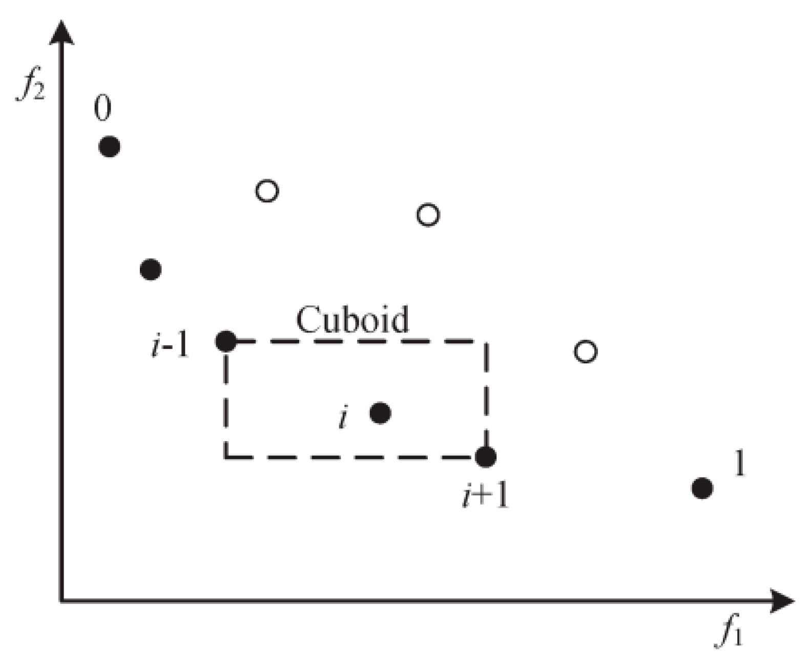
Crowding Distance

We define the sum of the distance differences between each individual and its neighbours on each subobjective function as the crowding distance of the individual. The crowding distance calculation can reflect the distribution of other solutions around each solution. The sum of the length and width of the dashed rectangle shown in Figure 1 is the crowding distance of individual i. In Figure 1, the crowding distances of the two individuals at both ends are set to infinity. In NSGA-II, individuals with large crowding distances have more opportunities to participate in reproduction and evolution to ensure that the algorithm can converge to a uniformly distributed Pareto surface, thereby maintaining the diversity of the population.

(3)

Genetic Strategy

First, we define the genetic parameter variables: population size $PS$, maximum number of genetic generations $T$, mutation probability $p_m$, and crossover probability $p_c$.

(a)

Solution encoding

Individual coding uses real vector coding. The capacity expansion value $y_a$ and speed limit value $s_a$ during different time periods in the network are used as the solution variables for real number vector coding.

(b)

Generation of the initial population

The number of members $PS$ in the initial group $P_0$ is generally 50–100, and this number can also be determined by trial-and-error calculation. The individual $PS$ of the initial group $P_0$ is randomly generated using the expansion constraints imposed on the road section capacity and the road section speed limit conditions.

(c)

Fitness evaluation

For each individual, the path-based double gradient projection algorithm is used to solve the lower-level variational inequality problem, and the order value and crowding distance of the individual are obtained through the nondominated sorting method and the crowding distance calculation. The smaller the individual’s order value, the higher the fitness. The greater the crowding distances of individuals with the same ordinal value, the higher the fitness.

(d)

Genetic manipulation

The operations of GAs generally include three basic types: selection, crossover, and mutation. From the initial group $PS$, $PS$ individuals are selected through the championship method to form the parent group $P_t$, and the crossover and mutation operations are performed on the parent group. Among them, the crossover operation uses the simulated binary crossover operator (SBX) on the parent individual encoded by the real number, randomly selects the crossover point for the two paired chromosomes, and then exchanges the parts after the crossover point to generate two new individuals. The mutation operation uses a polynomial mutation operator to select some genes from group $P_t$ according to the mutation probability $p_m$, which helps NSGA-II jump out of local optimal states.

(e)

Elitism selection

To maintain the diversity of individuals in the population, the nondominated ranking method and championship method are used to select $PS$ excellent individuals from the current generation $P_t$ and its children $Q_t$ to inherit the next generation. The selection process is as follows: the current generation $P_t$ and its children $Q_t$ are first combined into a new population $R_t$; nondominated sorting is performed on population $R_t$; the order value and crowding distance of each individual are calculated; and $PS$ excellent individuals are selected through the championship method.

The specific process of using NSGA-II to solve the biobjective optimization model is as follows:

Step 1.

Initialization. The population size $PS$, maximum algebra T, mutation probability $p_m$, crossover probability $p_c$, and other genetic parameters are set. The initial parent population $P_0$ is generated with a scale of $PS$$t=0$.

Step 2.

The individual fitness of population $P_0$ is evaluated, the individual order value and the crowding distance are obtained, and the individuals with order values of 1 form the initial optimal surface of the Pareto front.

Step 3.

Crossover and mutation operations are performed to generate the offspring population $Q_t$, the parent population $P_t$ and the offspring population $Q_t$ are combined to form the combined population $P_t$, and the individual fitness of $R_t$ is evaluated. The fusion of $R_t$ updates the current optimal surface of the Pareto front.

Step 4.

Using the method of competitive competition, $PS$ good individuals are selected from the combined population $R_t$ to form a new parent population $P_{t+1}$.

Step 5.

If $t<T,t=t+1$, the process reverts to Step 3; otherwise, the process advances to Step 6.

Step 6.

The optimal Pareto front is output, and the algorithm is terminated.

4. Numerical Examples

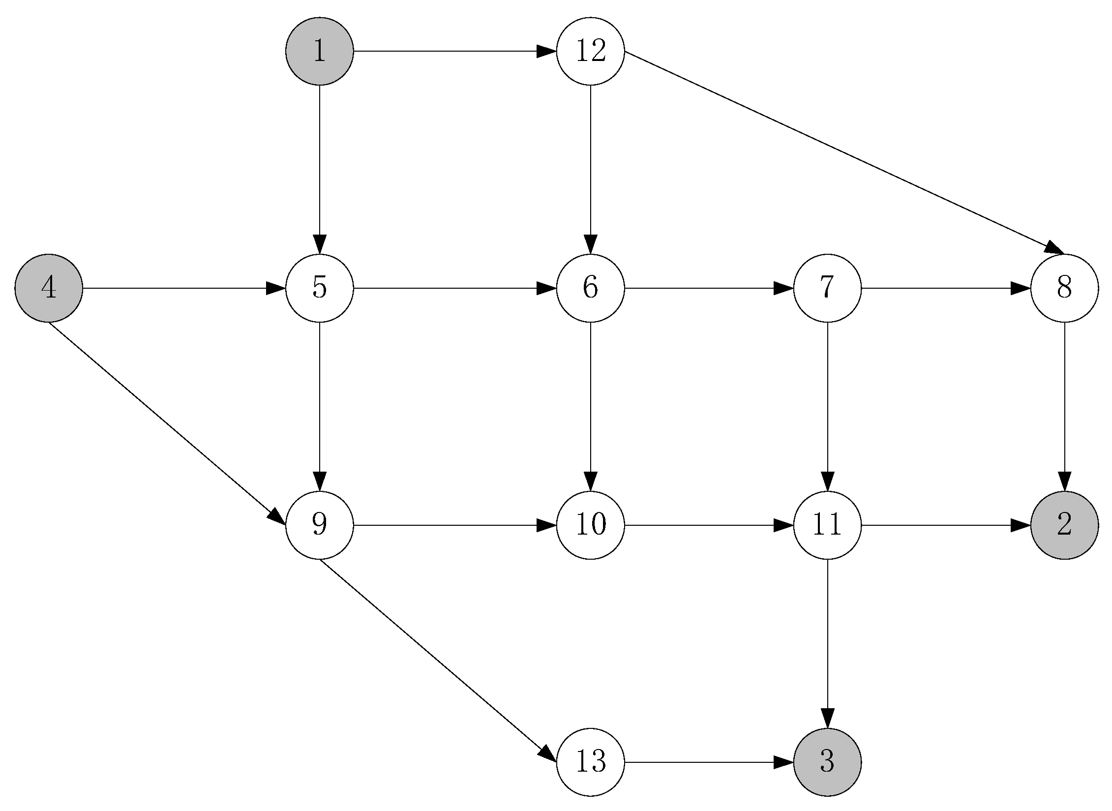
The network of Nguyen and Dupuis [36] illustrates the effectiveness of the above models and algorithms. The network consists of 4 ODs, 13 nodes, and 19 links, as shown in Figure 2. The parameters of the emission rate functions and the monetary valuation of each type of pollutant are shown in

Table 1. Parameters of the emission rate functions and the monetary valuation of each type of pollutant.

Section Number	Origin	Destination	${\mathit{t}}_{\mathit{a}}^0/\mathbf{min}$	${\mathit{C}}_{\mathit{a}}(\mathit{v}\mathit{e}\mathit{h}/\mathit{h})$	${\mathit{s}}_{\mathit{a}}^{\mathbf{max}}(\mathit{k}\mathit{m}/\mathit{h})$	${\overline{\mathit{s}}}_{\mathit{a}}(\mathit{k}\mathit{m}/\mathit{h})$	Section Length (m)	Number of Lanes
1	1	5	0.6	6000	60	-	600	3
2	1	12	0.45	6000	60	-	450	3
3	4	5	0.6	6000	60	-	600	3
4	4	9	0.6	6000	60	-	600	3
5	5	6	0.6	6000	60	-	600	3
6	5	9	0.6	6000	60	${\overline{s}}_6$	600	3
7	6	7	0.6	6000	60	-	600	3
8	6	10	0.6	6000	60	-	600	3
9	7	8	0.6	4000	60	-	450	2
10	7	11	0.45	6000	60	-	450	3
11	8	2	0.45	2000	60	-	450	1
12	9	10	0.6	6000	60	-	600	3
13	9	13	0.45	4000	60	${\overline{s}}_{13}$	450	2
14	10	11	0.45	6000	60	-	450	3
15	11	2	0.6	6000	60	-	600	3
16	11	3	0.6	6000	60	-	600	3
17	12	6	0.6	6000	60	-	600	3
18	12	8	1	2000	60	-	750	1
19	13	3	0.6	2000	60	-	600	1

, where all data are taken from Lo and Szeto [37]. The demand ratio among OD pairs 1–2, 1–3, 4–2, and 4–3 is 2:4:3:3, and the section capacity of each lane is 2000 pcu/h. The investment cost function is ${\mathrm{G}}_a(y_a)=3y_a{}^2$, and the congestion pricing function is ${\mathrm{G}}_a(g_a){=\mathrm{g}}_a$.

Speed limit control is carried out on sections 6 and 13; the speed limit in section 6 is within [52.17, 60.00], and the speed limit in section 13 is within [52.17, 60.00]. The OD demands during the morning peak, evening peak, and flat peak hours are 800 × 12, 700 × 12, and 600 × 12 vehicles/h, respectively. The constant pollution coefficients of different pollutants and their unit emission costs are shown in

Table 2. Parameters of the emission rate functions and the monetary valuation of each type of pollutant.

Section Length (m)	$\mathit{N}{\mathit{O}}_{\mathit{x}}$	$\mathit{V}\mathit{O}\mathit{C}$	$\mathit{C}\mathit{O}$
$A_m$	1.5718	2.7843	3.3963
$B_m$	0.040732	0.015062	0.014561
$C_m$	10,000	10,000	1000
${\eta }_m$ (EURO/kg)	13.80	2.95	0.01

.

${\mathrm{g}}_a=0$ solves the lower-level stochastic user balance model without considering the speed limit and road extension. We can obtain the traffic flow before road congestion charging is included, where we assume that the OD requirement is 800 × 12 vehicles/h.

Table 3. Flow without considering the speed limit of the flow assignment for the lower-level problem.

Section Number	$x_1$	$x_2$	$x_3$	$x_4$	$x_5$	$x_6$	$x_7$	$x_8$	$x_9$	$x_{10}$
Section Flow	1999.3	2800.7	3094.8	1705.2	3398.6	3022.7	911.9	1630.1	369.2	2496.9
Saturation	33.3%	46.7%	51.6%	28.4%	56.6%	50.4%	22.8%	27.2%	18.5%	41.6%
Section Number	$x_{11}$	$x_{12}$	$x_{13}$	$x_{14}$	$x_{15}$	$x_{16}$	$x_{17}$	$x_{18}$	$x_{19}$
Section Flow	2006.0	2110.8	1281.1	2400.0	4406.0	2718.9	1802.1	3797.9	1802.1
Saturation	33.4%	35.2%	64.1%	40.0%	73.4%	45.3%	45.1%	63.3%	90.1%	33.4%

shows the traffic flow and saturation of each section.

The saturation levels of sections 15 and 19 are 73.4% and 90.1%, respectively. Since they are clearly crowded, we can use congestion charges on road sections 15 and 19, which can change passenger travel paths and alleviate the congestion in these road sections. Assuming that we charge ${\mathrm{g}}_{15}$ and ${\mathrm{g}}_{19}$ in sections 15 and 19, respectively, we use the expression of the road congestion pricing constraint (4.20), and the pricing range is set as [0–27], [0–36].

4.1. Comparison of User Equilibrium Results

We use the lower flow model with the SUE model to describe travellers’ route choice behaviours. Compared with UE, the flow of the SUE assignment model accounts for travellers through their travel choices and personal understandings of random travel path. We use two cases to show the difference between SUE and UE.

The traffic network and road section parameters are similar to those in the previous sections. We assume that the unit traffic demand is 800, the nest size parameter u in the random user equilibrium distribution (SUE) is 0.5, the sensitivity of path selection to the path cost $\theta$ is 1, and the path similarity parameter of traveller selection $\gamma$ is 1. The stop parameter in the user balance distribution is set as $\xi ={10}^{-6}$.

Table 4. The traffic assignment results yielded by UE and SUE.

Section Number	Origin	Destination	UE Configuration Results			SUE Configuration Results
			Flow	Time Remaining	System Impedance	Flow	Time Remaining	System Impedance
1	1	5	4234.7	0.466	1974.21	1999.3	0.451	901.36
2	1	12	565.3	0.600	339.20	2800.7	0.604	1692.37
3	4	5	0	0.600	0	3094.8	0.606	1876.57
4	4	9	4800	0.637	3056.95	1705.2	0.601	1024.14
5	5	6	0	0.600	0	3398.6	0.609	2070.63
6	5	9	2634.7	0.602	1585.39	3022.7	0.606	1831.12
7	6	7	0	0.450	0	911.9	0.450	410.52
8	6	10	2634.7	0.603	1589.16	1630.1	0.600	978.87
9	7	8	1600	0.796	1273.73	369.2	0.750	276.95
10	7	11	565.3	0.600	339.20	2496.9	0.603	1504.86
11	8	2	0	0.600	0	2006.0	0.601	1205.88
12	9	10	2634.7	0.451	1189.04	2110.8	0.451	952.03
13	9	13	1600	0.478	764.24	1281.1	0.461	591.05
14	10	11	2400	0.602	1445.55	2400.0	0.602	1445.50
15	11	2	2400	0.453	1087.3	4406.0	0.470	2069.18
16	11	3	2400	0.602	1445.53	2718.9	0.604	1641.66
17	12	6	2965.3	0.471	1397.56	1802.1	0.453	815.98
18	12	8	2634.7	0.603	1589.19	3797.9	0.614	2333.58
19	13	3	2965.3	1.054	3126.67	1802.1	0.659	1188.21
System travel impedance			22,202.92			24,810.46

shows the speed limit and road congestion charging case based on the SUE and UE flow allocations. The traffic assignment method based on SUE avoids the large sensitivity problem. Although the impedance based on SUE is larger than that based on UE, the traffic flow is more even when using SUE.

4.2. Parametric Analysis

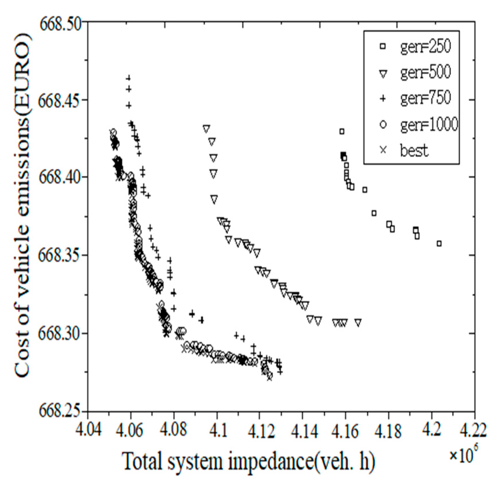
According to the biobjective GA, a traffic network design model based on the UE allocation is solved. The algorithm parameters are set as follows: the population size $ps=100$, number of evolutionary iterations $gen=1000$, crossover probability $p=0.9$, mutation probability $q=0.1$, and stop parameter $\xi ={10}^{-6}$. We set the model parameters as follows: the investment matching coefficient $\theta =0.001$, matching coefficient for congestion charging $\tau =0.5$, and understanding parameter $\mathrm{u}=0.5$. Every 250 iterations, we record the current nondominated solution set. Figure 3 shows the comparison of the Pareto fronts obtained under different numbers of iterations. It can be found that the more iterations there are, the closer the Pareto front obtained by NSGA-II is to the optimal Pareto front. When the number of iterations reaches 1000, NSGA-II is able to achieve optimal results.

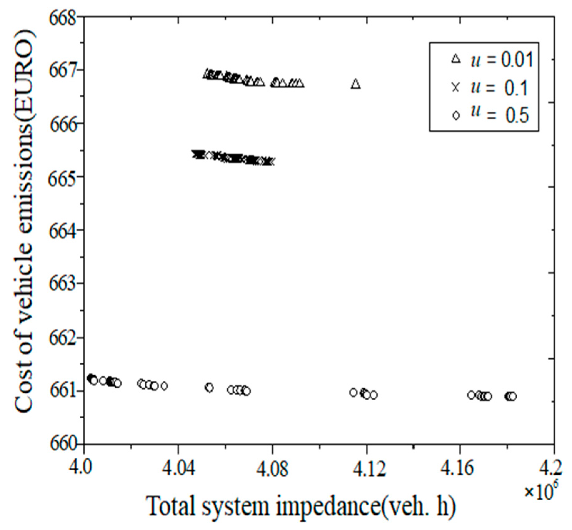
Travel understanding parameters represent the sensitivity of travellers’ path selections and path costs. The values of different understanding parameters can be regarded as the errors between the traveller’s understanding of the trip cost and the actual travel cost. The approximate Pareto optimal frontiers yielded when the understanding parameter u is 0.01, 0.1, and 0.5 under the same algorithm parameter settings are shown in Figure 4. The higher the value of the understanding parameter u, the smaller the error of the traveller’s perception of the path cost, and vice versa. Figure 4 shows that when the coefficient of u rises from 0.01 to 0.1 and 0.5 in the process of traffic network exhaust pollutant emission decline, the impedance of the traffic network falls, and the traveller’s path perception error is smaller, so the traveller can more effectively choose the path with the optimal cost.

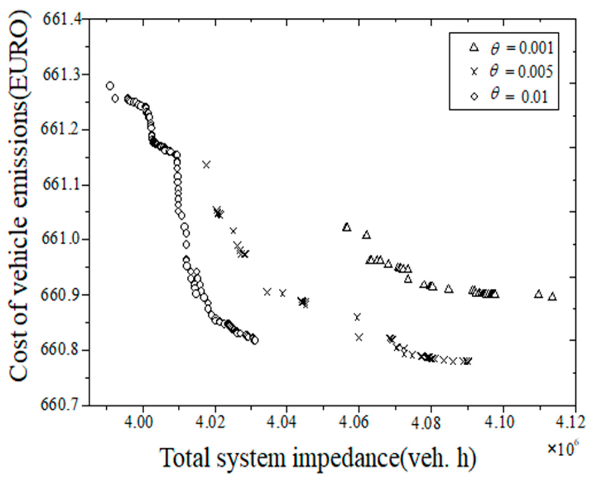
The investment matching coefficient $\theta$ in the upper optimization model represents the conversion coefficient that matches the investment expense to the travel time of the system. Different values of the investment matching coefficient can be regarded as the trade-off made by traffic planners to improve the traffic network to the greatest extent while reducing the investment expense as much as possible. The approximate Pareto optimal frontiers yielded when the investment matching coefficient $\theta$ is 0.001, 0.005, and 0.01 under the same algorithm parameter settings are shown in Figure 5. Figure 5 shows that when the matching coefficient $\theta$ drops to 0.01, 0.005, and 0.001, the total impedance of the traffic network decreases continuously, and the total emissions of exhaust pollutants also decrease continuously.

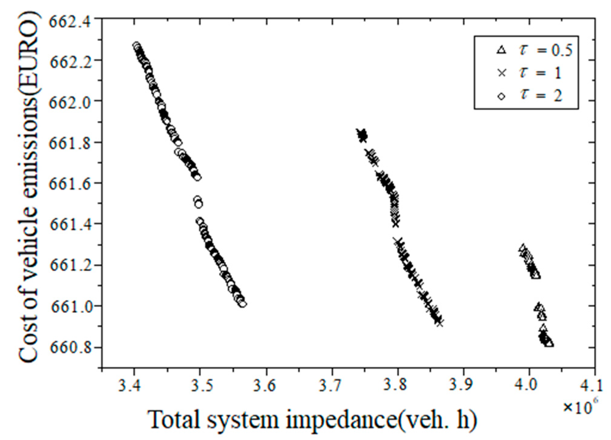
The matching coefficient for congestion charging $\tau$ represents the conversion coefficient of the system travel time. The different values of the matching coefficient for charging can be regarded as a trade-off between traffic managers’ efforts to minimize road congestion and increase the travel impedance of the given road section for travellers. The approximate Pareto optimal frontiers yielded when the matching coefficient for charging $\tau$ is 0.5, 1, and 2 under the same algorithm parameter settings are shown in Figure 6. The larger the charging matching coefficient, the stricter the management control of the congestion charging section. The smaller the charging matching coefficient, the looser the management control. In Figure 6, when the matching coefficient $\tau$ drops to 2, 1, and 0.5, the total impedance of the traffic network decreases continuously, as do the total emissions of exhaust pollutants.

4.3. Speed Limit Control Comparison during Different Periods

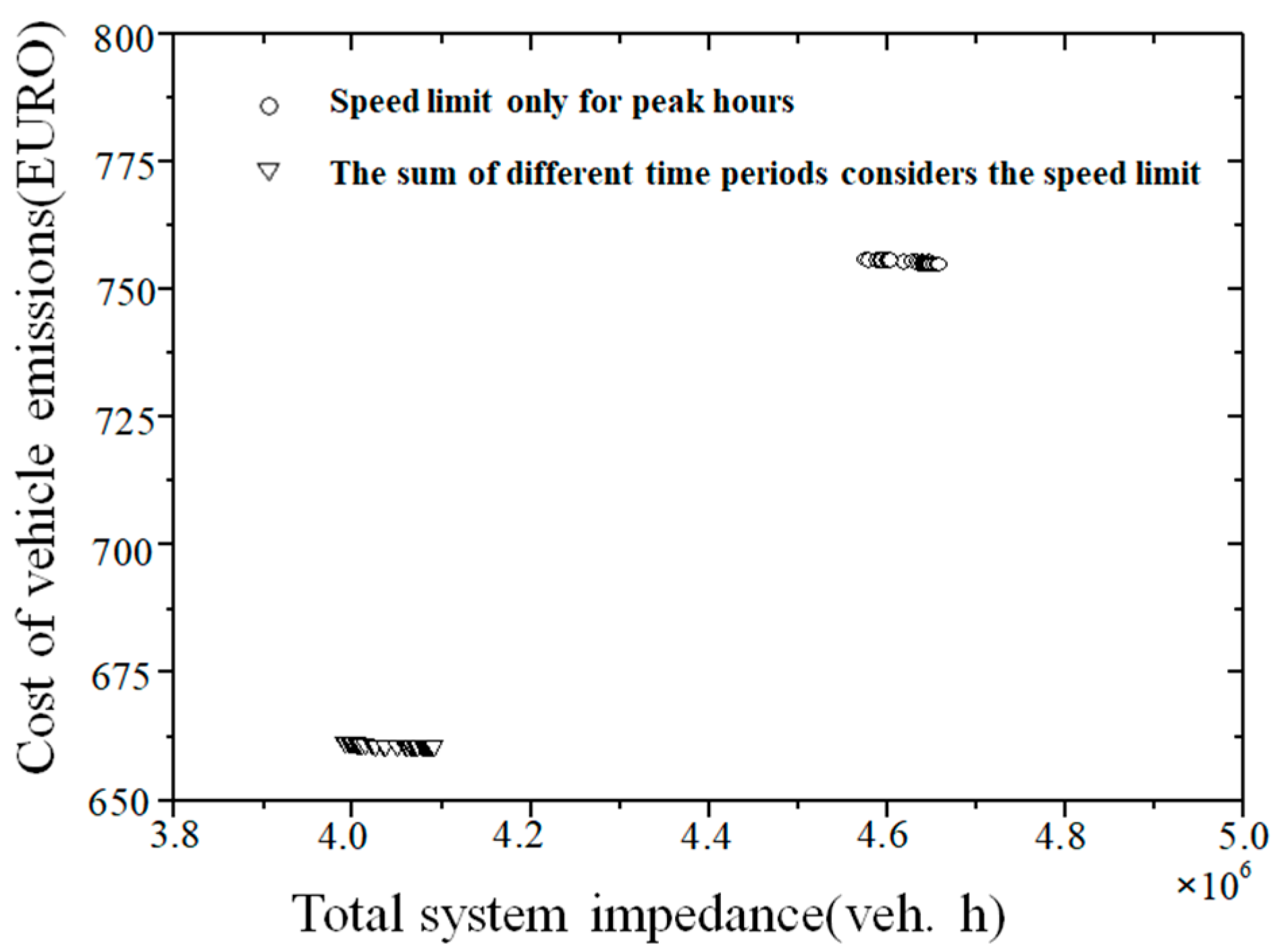
We consider the differences in traffic demand levels during different periods and set speed limits in different periods. The model parameter settings are: the investment matching coefficient $\theta =0.001$, the matching coefficient for congestion charging $\tau =0.5$, and the understanding parameter $\mathrm{u}=0.5$. Two situations are compared: setting the speed limits during peak hours separately and setting the speed limit during each period comprehensively. The approximate Pareto optimal fronts yielded in these two cases are shown in Figure 7. Setting a speed limit can significantly improve the efficiency of urban network traffic and reduce urban traffic pollution by comprehensively considering the traffic conditions inherent in various periods.

4.4. Comparative Effects Analysis Regarding Congestion Pricing

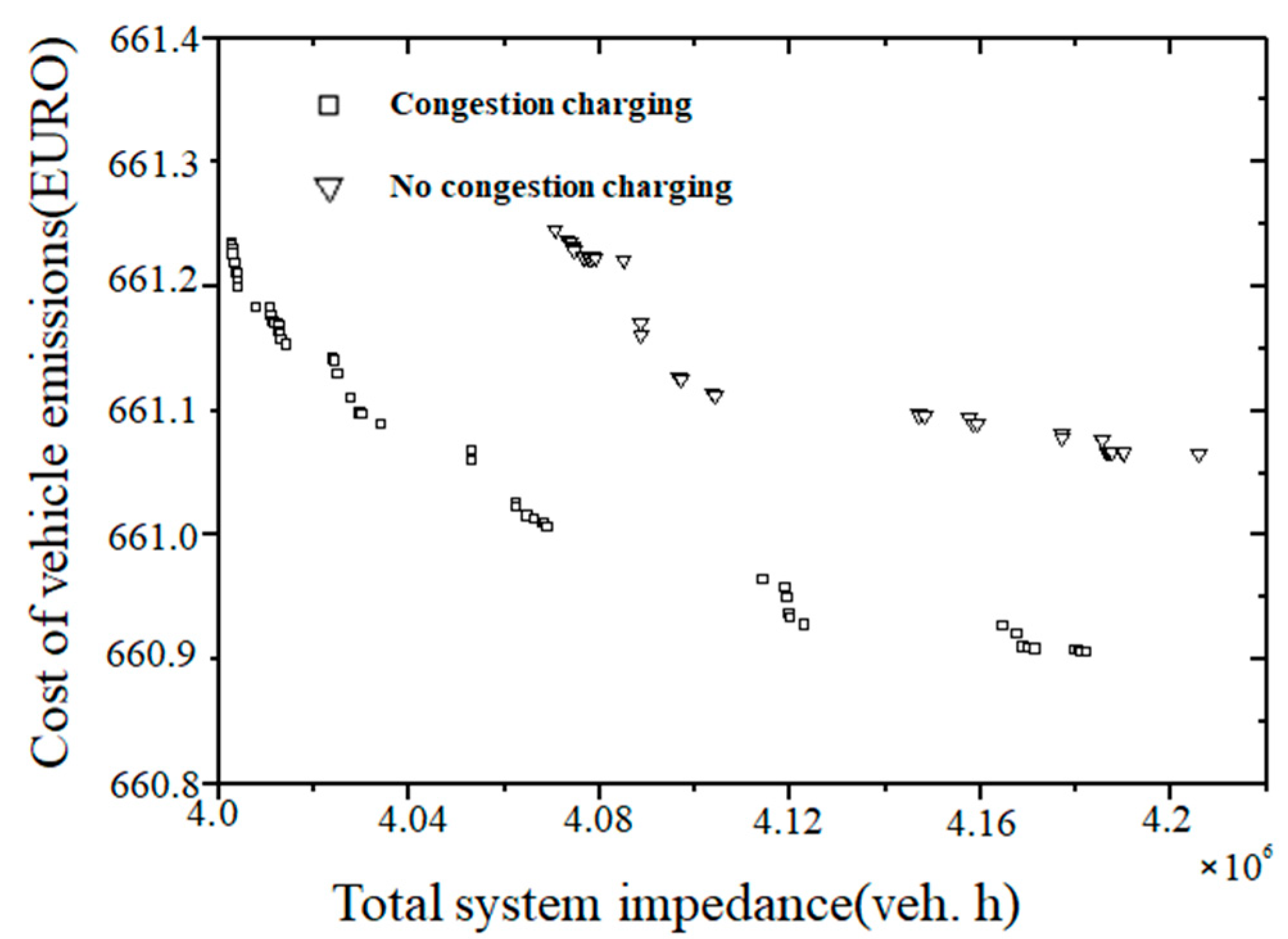
The traffic control strategy of road congestion pricing is added to reduce the traffic demand of congested sections and improve the operating efficiency of the whole network. The investment matching coefficient $\theta =0.001$, the matching coefficient for congestion charging $\tau =0.5$, and the understanding parameter $\mathrm{u}=0.5$. The parameter setting compares the implementation of the road congestion charging strategy with the speed limit and the noncharging congestion management approach. The approximate Pareto optimal fronts for these two situations are shown in Figure 8. The average saturation levels of sections 15 and 19 decrease to 35.2% and 50.8%, respectively. Based on a comparison of the situations before and after charging, charging for crowded roads can change the travel paths of travellers and alleviate road congestion. This also shows that the implementation of the road congestion charging management strategy can improve the traffic efficiency of the entire city network.

5. Conclusions

In this paper, based on the traffic network design problem with the consideration of speed limits, a method of road congestion charging is proposed to guide residents’ travel decisions. This paper also establishes a congested road charging model based on SUE to alleviate road congestion and reduce pollution. We use NSGA-II to solve this bilevel programming problem. The lower-level SUE allocation problem uses the adaptive weighted average method, which is analysed through a simple calculation example. From the obtained results, the SUE-based traffic allocation method avoids the problem of excessive sensitivity in deterministic traffic allocation situations. Although the total impedance of the traveller system obtained by using the SUE-based traffic distribution model is larger than that based on UE, the SUE-based traffic distribution is more uniform. Analyses of the results regarding calculation examples and key parameters effectively prove the applicability of the proposed algorithm and model. The innovation of this paper is to study the speed limit in the continuous traffic network design problem while adding the control strategy of road congestion charging. After the implementation of the road congestion charging management method, the two situations of implementing the road congestion charging strategy and the noncongestion charging management under the condition of the speed limit were compared by setting and adjusting the relevant parameters. It was concluded that the saturation of the corresponding road section under different conditions was reduced by 35.2% and 50.8%, respectively. By comparing the situations before and after the toll, charging the congested road is found to effectively alleviate the operating condition of the congested road section and improve the traffic efficiency of the entire city network.

References

- Abdulaal, M.; LeBlanc, L. Continuous equilibrium network design models. Transp. Res. Part B 1979, 13, 19–32. [Google Scholar] [CrossRef]
- Yang, H.; Bell, M.G.H. Models and algorithms for road network design: A review and some new developments. Transp. Rev. 1998, 18, 257–278. [Google Scholar] [CrossRef]
- Yang, H.; Bell, M.G.H. Special issue: Transportation bilevel programming problems: Recent methodological advances. Transp. Res. Part B 2001, 35, 1–4. [Google Scholar] [CrossRef]
- Li, C.; Yang, H.; Zhu, D.; Meng, Q. A global optimization method for continuous network design problems. Transp. Res. Part B 2012, 46, 1144–1158. [Google Scholar] [CrossRef]
- Meng, Q.; Yang, H.; Bell, M. An equivalent continuously differentiable model and a locally convergent algorithm for the continuous network design problem. Transp. Res. Part B 2001, 35, 83–105. [Google Scholar] [CrossRef]
- Xu, T.; Wei, H.; Hu, G. Study on continuous network design problem using simulated annealing and genetic algorithm. Expert Syst. Appl. 2009, 36, 1322–1328. [Google Scholar] [CrossRef]
- Mathew, T.; Sharma, S. Capacity expansion problem for large urban transportation networks. J. Transp. Eng. 2009, 135, 406–415. [Google Scholar] [CrossRef]
- Gao, Z.; Sun, H.; Zhang, H. A globally convergent algorithm for transportation continuous network design problem. Optim. Eng. 2007, 8, 241–257. [Google Scholar] [CrossRef]
- Wang, D.; Lo, H. Global optimum of the linearized network design problem with equilibrium flows. Transp. Res. Part B 2010, 44, 482–492. [Google Scholar] [CrossRef]
- Farahani, R.; Miandoabchi, E.; Szeto, W.; Rashidi, H. A review of urban transportation network design problems. European J. Oper. Res. 2013, 229, 281–302. [Google Scholar] [CrossRef] [Green Version]
- Baskan, O. Determining Optimal Link Capacity Expansions in Road Networks Using Cuckoo Search Algorithm with Lévy Flights. J. Appl. Math. 2013, 2013, 1–11. [Google Scholar] [CrossRef]
- Baskan, O. An evaluation of heuristic methods for determining optimal link capacity expansions on road networks. Int. J. Transp. 2013, 2, 77–94. [Google Scholar] [CrossRef]
- Karoonsoontawong, A.; Waller, S. Dynamic continuous network design problem-Linear bilevel programming and metaheuristic approaches. Transp. Res. Rec. 2006, 1964, 104–117. [Google Scholar] [CrossRef]
- Wu, Y.; Yang, H.; Tang, J.; Yu, Y. Multi-objective re-synchronizing of bus timetable: Model, complexity and solution. Transp. Res. Part C 2016, 67, 149–168. [Google Scholar] [CrossRef]
- Lu, J.; Yang, Z.; Timmermans, H.; Wang, W. Optimization of airport bus timetable in cultivation period considering passenger dynamic airport choice under conditions of uncertainty. Transp. Res. Part C 2016, 67, 15–30. [Google Scholar] [CrossRef]
- Davis, G. Exact local solution of the continuous network design problem via stochastic user equilibrium assignment. Transp. Res. Part B 1994, 28, 61–75. [Google Scholar] [CrossRef]
- Liu, H.; Wang, D. Global optimization method for network design problem with stochastic user equilibrium. Transp. Res. Part B 2015, 72, 20–39. [Google Scholar] [CrossRef]
- Du, B.; Wang, D. Solving continuous network design problem with generalized geometric programming approach. Transp. Res. Record. 2016, 2567, 38–46. [Google Scholar] [CrossRef] [Green Version]
- Long, J.; Gao, Z.; Zhang, H.; Szeto, W. A turning restriction design problem in urban road networks. Eur. J. Oper. Res. 2010, 206, 569–578. [Google Scholar] [CrossRef] [Green Version]
- Gallo, M.; D’Acierno, L.; Montella, B. A meta-heuristic approach for solving the Urban Network Design Problem. Eur. J. Oper. Res. 2010, 201, 144–157. [Google Scholar] [CrossRef]
- Zhang, S.; Li, J.; Li, L. Study speed of vehicles for road traffic accident. Commun. Stand. 2006, 8, 1–2. [Google Scholar]
- Lave, C.; Elias, P. Resource allocation in public policy: The effects of the 65-mph speed limit. Econ. Inq. 1997, 35, 614–620. [Google Scholar] [CrossRef]
- Liu, W.; Yin, Y.; Yang, H. Effectiveness of variable speed limits considering commuters’ long-term response. Transp. Res. Part B Methodol. 2015, 81, 498–519. [Google Scholar] [CrossRef]
- Sun, J.; Shen, J.; Liu, Y. Variable speed limits strategy of urban expressway. J. Highw. Transp. Res. Dev. 2012, 29, 98–103. [Google Scholar]
- Yang, H.; Wang, X.; Yin, Y. The impact of speed limits on traffic equilibrium and system performance in networks. Transp. Res. Part B 2012, 46, 1295–1307. [Google Scholar] [CrossRef]
- Madireddy, M.; De Coensel, B.; Can, A.; Degraeuwe, B.; Beusen, B.; De Vlieger, I.; Botteldooren, D. Assessment of the impact of speed limit reduction and traffic signal coordination on vehicle emissions using an integrated approach. Transp. Res. Part D 2011, 16, 504–508. [Google Scholar] [CrossRef] [Green Version]
- Yan, C.Y.; Jiang, R.; Gao, Z.Y.; Shao, H. Effect of speed limits in degradable transport networks. Transp. Res. Part C 2015, 56, 94–119. [Google Scholar] [CrossRef]
- Yang, H.; Ye, H.; Li, X.; Zhao, B. Speed limits, speed selection and network equilibrium. Transp. Res. Part C 2015, 51, 260–273. [Google Scholar] [CrossRef]
- Chen, X.; Wang, Y.; Zhang, Y. A Trial-and-Error Toll Design Method for Traffic Congestion Mitigation on Large River-Crossing Channels in a Megacity. Sustainability 2021, 13, 2749. [Google Scholar] [CrossRef]
- Cheng, Q.; Chen, J.; Zhang, H.; Liu, Z. Optimal Congestion Pricing with Day-to-Day Evolutionary Flow Dynamics: A Mean–Variance Optimization Approach. Sustainability 2021, 13, 4931. [Google Scholar] [CrossRef]
- Chen, Y.; Zheng, N.; Hai, L. A novel urban congestion pricing scheme considering travel cost perception and level of service. Transp. Res. Part C 2021, 125, 103042. [Google Scholar] [CrossRef]
- Alkaa, F.; Diabat, A.; Elhedhli, S. A Lagrangian heuristic and GRASP for the hub-and-spoke network system with economies-of-scale and congestion. Transp. Res. 2019, 102, 249–273. [Google Scholar]
- Aya, A.; Baher, A. A bi-level distributed approach for optimizing time-dependent congestion pricing in large networks: A simulation-based case study in the Greater Toronto Area. Transp. Res. Part C 2017, 85, 684–710. [Google Scholar]
- Baskan, O.; Ozan, C.; Dell’Orco, M.; Marinelli, M. Improving the Performance of the Bilevel Solution for the Continuous Network Design Problem. Promet-Traffic Transp. 2018, 30, 709–720. [Google Scholar] [CrossRef]
- Deb, K.; Agrawal, S.; Pratap, A.; Meyarivan, T. A fast elitist non-dominated sorting genetic algorithm for multi-objective optimization: NSGA-II. Lect. Notes Comput. Sci. 2000, 1917, 849–858. [Google Scholar]
- Nguyen, S.; Dupuis, C. An efficient method for computing traffic equilibria in networks with asymmetric transportation costs. Transp. Sci. 1984, 18, 185–202. [Google Scholar] [CrossRef]
- Hong, K.; Szeto, W. A cell-based variational inequality formulation of the dynamic user optimal assignment problem. Transp. Res. Part B 2002, 36, 421–443. [Google Scholar]
Figure 1.
Illustration of the crowd distance.
Figure 2.
The network of Nguyen and Dupuis.
Figure 3.
The Pareto frontiers for different periods of the column generation procedure.
Figure 4.
The Pareto frontiers for different perceived parameters.
Figure 5.
The Pareto frontiers for different investment matching coefficients.
Figure 6.
The Pareto frontiers for different congestion pricing matching coefficients.
Figure 7.
The Pareto frontiers obtained when considering speed limits during different peak periods only.
Figure 8.
The Pareto frontiers obtained based on whether congestion charging is implemented.