Predictive Modeling Approach for Surface Water Quality: Development and Comparison of Machine Learning Models

Abstract

Water pollution is an increasing global issue that societies are facing and is threating human health, ecosystem functions and agriculture production. The distinguished features of artificial intelligence (AI) based modeling can deliver a deep insight pertaining to rising water quality concerns. The current study investigates the predictive performance of gene expression programming (GEP), artificial neural network (ANN) and linear regression model (LRM) for modeling monthly total dissolved solids (TDS) and specific conductivity (EC) in the upper Indus River at two outlet stations. In total, 30 years of historical water quality data, comprising 360 TDS and EC monthly records, were used for models training and testing. Based on a significant correlation, the TDS and EC modeling were correlated with seven input parameters. Results were evaluated using various performance measure indicators, error assessment and external criteria. The simulated outcome of the models indicated a strong association with actual data where the correlation coefficient above 0.9 was observed for both TDS and EC. Both the GEP and ANN models remained the reliable techniques in predicting TDS and EC. The formulated GEP mathematical equations depict its novelty as compared to ANN and LRM. The results of sensitivity analysis indicated the increasing trend of input variables affecting TDS as HCO₃⁻ (22.33%) > Cl⁻ (21.66%) > Mg²⁺ (16.98%) > Na⁺ (14.55%) > Ca²⁺ (12.92%) > SO₄²⁻ (11.55%) > pH (0%), while, in the case of EC, it followed the trend as HCO₃⁻ (42.36%) > SO₄²⁻(25.63%) > Ca²⁺ (13.59%) > Cl⁻ (12.8%) > Na⁺ (5.01%) > pH (0.61%) > Mg²⁺ (0%). The parametric analysis revealed that models have incorporated the effect of all the input parameters in the modeling process. The external assessment criteria confirmed the generalized outcome and robustness of the proposed approaches. Conclusively, the outcomes of this study demonstrated that the formulation of AI based models are cost effective and helpful for river water quality assessment, management and policy making.

1. Introduction

Surface water is the most sensitive and vulnerable resource since its demand increases with the rise in population. The surface water bodies are abundantly available which fulfill multiple needs such as industrial processes, drinking, irrigation, agricultural production and hydroelectricity generation. The streams, lakes and rivers are the most susceptible to pollution, receiving more waste load from other sources attributed to their dynamic nature and easy accessibility. Major processes responsible for water quality degradation include urban waste water, non-treatment sewage discharge, industrial processes, hazardous substances, diffuse pollution from agricultural lands, climatic processes and anthropogenic activities [1,2,3]. Polluted water is a major issue threatening human health, agriculture and ecosystems [4].

Estimating the processes pertaining to water quality deterioration is becoming a key hurdle in managing pollution of the marine environment [5,6]. The selected variables for water quality assessment are total dissolved solids (TDS) and specific conductivity (EC). Both TDS and EC depend on organic matter and inorganic salts dissolved in water. A variation in TDS or EC level is a sign of source pollution, hence, elevated values of these parameters indicate contamination in water [7,8]. The field monitoring and manual laboratory tests/calculations methods for water quality assessment are labor-intensive and time-consuming [9]. In order to condense the experimental workload for the calculation of water quality parameters, modeling techniques can be the best alternatives. Employing computer aided models for modeling the significant properties of water are helpful in saving time, cost and also making suitable predictions [10,11]. Modeling and estimation in different fields were carried out with typical and conventional computing methods including numerical, and deterministic models. Although, these models have limited capability and are complex in structure (require in depth details). Therefore, leaves a gap to use alternate and advanced modeling approaches [12,13].

The artificial intelligence (AI) techniques encompassing neural network (ANN), random forest (RF), multi-expression programming (MEP), adaptive neuro-fuzzy inference-based system (ANFIS) and gene expression programming (GEP) remained the reliable methods for valuable predictions and solving complex problems in various engineering domains [9,10,14,15,16,17,18,19,20,21,22,23,24]. The ANN was defined as enormous parallel spread processors containing simple units [25]. The hidden network between the neurons are adjusted in a way to develop and store the information required for modeling the complex systems [19]. Some drawbacks of ANN include unexplained behavior and difficulty in determining the proper network structure. The ANN does not give information regarding the adopted procedure, thus reducing the trust in the network structure [26,27]. The Genetic Programing (GP) was presented as a simplification of genetic algorithm [28]. In gene expression programming (GEP), which is the enhanced form of GP, the formation of genetic diversity is very simplified because the process works at chromosomes level [29]. The linear regression models (LRM) are the oldest and frequently used models across many fields. These are statistical tools that creates a relation between several independent and a single dependent variable [30].

Various researchers used different models for the estimation of water quality parameters. Palani et al. (2008) [16] used ANN to forecast dissolved oxygen (DO), salinity, temperature and chlorophyll-a in Singapore coastal water. The authors reported excellent prediction capability of the ANN model with correlation coefficient ranging from 0.8 to 0.9. Ahmed et al. (2019) [31] used ANFIS, radial bias function and multi-layer perception neural network models along with wavelet data de-noising technique in predicting pH, suspended solids and ammoniacal nitrogen concentration. The authors reported improved performance of the predictive models with data de-noising technique. Marti et al. (2013) [19] used ANN, GEP and regression for DO prediction in sand media filters utilizing 769 data points from experimental results. EC, pH, dissolved oxygen and head loss remained the most effective parameters. The results exposed better estimation of GEP model than other techniques. Granata et al. (2017) [32] predicted total suspended solids (TSS), biochemical oxygen demand (BOD), chemical oxygen demand (COD) and TDS of wastewater in a drainage basin with the help of support vector regression (SVR) and regression tree (RT) models. The authors reported better performance of SVR than RT in predicting the targeted output. The ANN was used by Sarkar et al. (2015) [14] for DO prediction. The authors reported accurate results of ANN with correlation coefficient close to 0.9. Haghiabi et al. (2018) [33] employed SVM, ANN and group method of data handling (GMDH) models in predicting various water quality parameters. The authors demonstrated suitable performance of both ANN and SVM for water quality prediction. Zhang et al. (2019) [34] used hybrid neural network model to predict water treatment plant production capacity. The results of the study demonstrated enhanced performance of the model by using a larger dataset.

The AI and machine learning modeling techniques were successfully employed in the aforementioned studies. A literature survey demonstrated that most of the modeling studies rely only on limited duration data and/or limited number of data points. Therefore, a systematic and detailed analysis is needed to consider the behavior of AI and regression-based techniques using a large dataset. Most of the modeling methodologies reported in literature have low and uneven prediction capacity due to the use of inadequate dataset. Moreover, limited research is available that focuses on the use of models that are efficient to provide empirical expressions. Such modeling approaches will ultimately reduce the experimental workload in predicting important water quality variables.

A study conducted by Shah et al. (2021) [8], where ANFIS modeling was applied in predicting the monthly TDS and EC in upper Indus river basin (UIB) measured at Bisham Qilla gauging station. The ANFIS model was coupled with data preprocessing and input optimization routine to remove the outliers and to select the most influential input combination. The authors reported an excellent result of the ANFIS model in TDS and EC prediction. In comparison to the aforementioned study, the present study is mainly devoted to applying AI and regression methods for modeling TDS and EC in the expanded study region. The dataset, simultaneously measured at both Doyian and Bisham Qilla outlets, were utilized for models training and testing. Thereafter, a comparative assessment is conducted in selecting the best model. The employed techniques included artificial neural network (ANN), gene expression programming (GEP) and linear regression model (LRM) utilizing monthly historical data. Models were developed for TDS and EC and performance was assessed by computing statistical indicators. Variable importance and a parametric study were conducted to figure out the influence of modeling inputs on the targeted output. The results of the present study might provide a valuable insight to authorities to devise a strategy for the effective management of river water quality.

2. Material and Methods

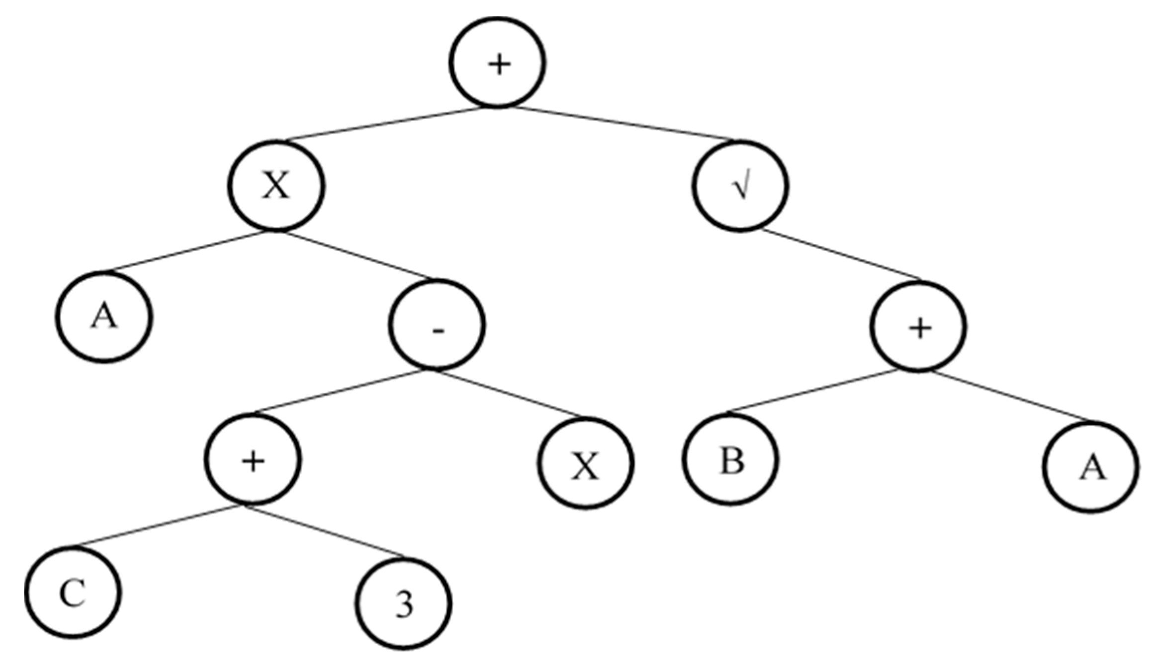
2.1. Genetic Base Algorithm

The enhanced variant of genetic programming (GP) was developed by Ferreira, C. [35], which is known as gene expression programming (GEP). A parse tree structure is coded in GEP which overcome the limitations of the GP [36]. Due to multigenic behavior, GEP uses unpretentious criteria for genetic variety formation which enable them to develop nonlinear and complex programs. GEP process is composed of various sets such as parameter set, fitness measure set, function set, criteria set and terminal set. The two main components of GEP are the chromosomes and expression trees (ETs). The ETs are used to express different nonlinear individuals and the genetic information encoded in the chromosomes. ETs are an excellent way to represent an expression in a computer because ET can be easily evaluated as compared to genetic information and equations [37]. A typical example of ET is shown in Figure 1. Furthermore, during the reproduction stage, the genetic operators are commonly used to modify the chromosomes [38,39]. GEP can represent any parse tree because of the capability of producing chromosomes. For such purpose, a new language called Karwa language is used to decode the information in the chromosomes [40,41]. An empirical relationship between the chromosomes and sets can be develop using the expression called Karva notation. The K expression from Karwa notation can be converted into mathematical equations that have the proficiency to forecast the output as a function of input variables and are applicable with high accuracy [21]. For GEP model development, the GeneXpro software tool was used and the GEP modeling parameters are listed in

Table 1. Best fitted parameters for GEP algorithm run.

Parameter	Setting
Number of Chromosomes	30
Number of Genes	4
Head size	10
Gene size	26
Linking function	Addition
Function set	+ , ̶ , × , ÷ , ^2 , 3√
Mutation rate	0.0138
Inversion rate	0.00546
Constants per gene	10
Maximum complexity	10
Data type	Floating type
Lower bound	−10
Upper bound	10

.

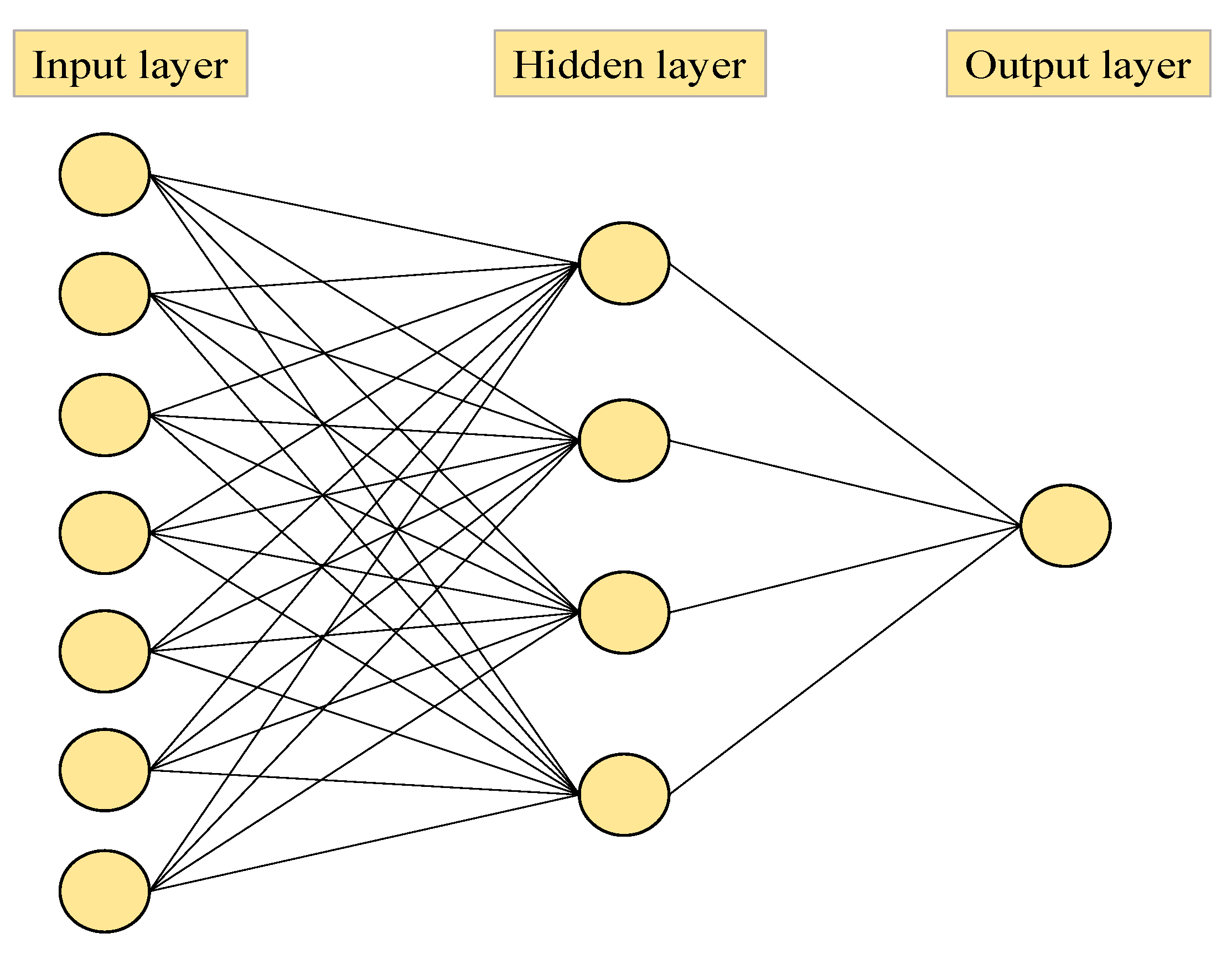
2.2. Artificial Neural Network (ANN)

The artificial neural network (ANN) was introduced by McCulloch et al. (1943) [42]. The use of ANN in modeling studies begins with the development of back propagation training algorithm in 1986 [43]. The artificial neuron is the basic element for simulation of biological nervous system microstructures. ANN has the ability to portray the nonlinear and complex functionalities in term of some variables to train the structure [16]. Figure 2 shows the architecture of typical ANN with different form of layers. Based on agreeable training, the ANN replicate the output based on unseen input data. Recently, the applications of ANN have been extended to many fields including water quality modeling, temperature prediction, ground water and hydrologic processes modeling [7,15,44]. In this study, the ANN model i.e., feed forward neural network type, was developed in the MATLAB environment. The final optimum parameters set for ANN modeling employed in the current study, are listed in

Table 2. Parameters of ANN for optimal network configuration.

Parameter	Fitted Value
	TDS	EC
Training dataset	252 (70%)	252 (70%)
Testing dataset	108 (30%)	108 (30%)
General
Network type	Feed forward neural network
Data division	Random
Number of hidden neurons	10
Training algorithm	Levenberg-Marquardt
Transfer function for hidden layer	TANSIG
Transfer function for output layer	PURELIN
Number of nonlinear parameters	18
Number of epochs	35
Learning rate	0.01

.

2.3. Linear Regression Model (LRM)

Linear regression modeling (LRM) applies a linear approach to model the relationship between a scalar and one or more explanatory variables. In linear regression modeling, a linear predictor function is used, whose unknown parameters are estimated from the given data. In this method, one variable is considered as explanatory variable, while the other one is considered to be a dependent variable. It is a frequently used method with practical applications in various fields of engineering. The generated regression-based equations can further be used specifically for water related problems [45]. Below, Equations (1) and (2) representing the mathematical form of linear regression analysis [46,47].

Y = a + β₁X₁ + β₂X₂ +⋯⋯ + β_iX_i

(1)

Y = a + β₁X_i + β₂X_j + β₃X_i² + β₄X_j² + ⋯⋯ + β_kX_iX_j

(2)

In both the Equations, a is the intercept, β is the slope or coefficient and k is the number of observations. The linear regression fit an estimated model to a dataset of Y and X values and the fitted model may be used to estimate Y with the addition of known X values [46]. The LRM employed in this study was developed using statistical package for social sciences (SPSS).

3. Study Area, Datasets and Modeling

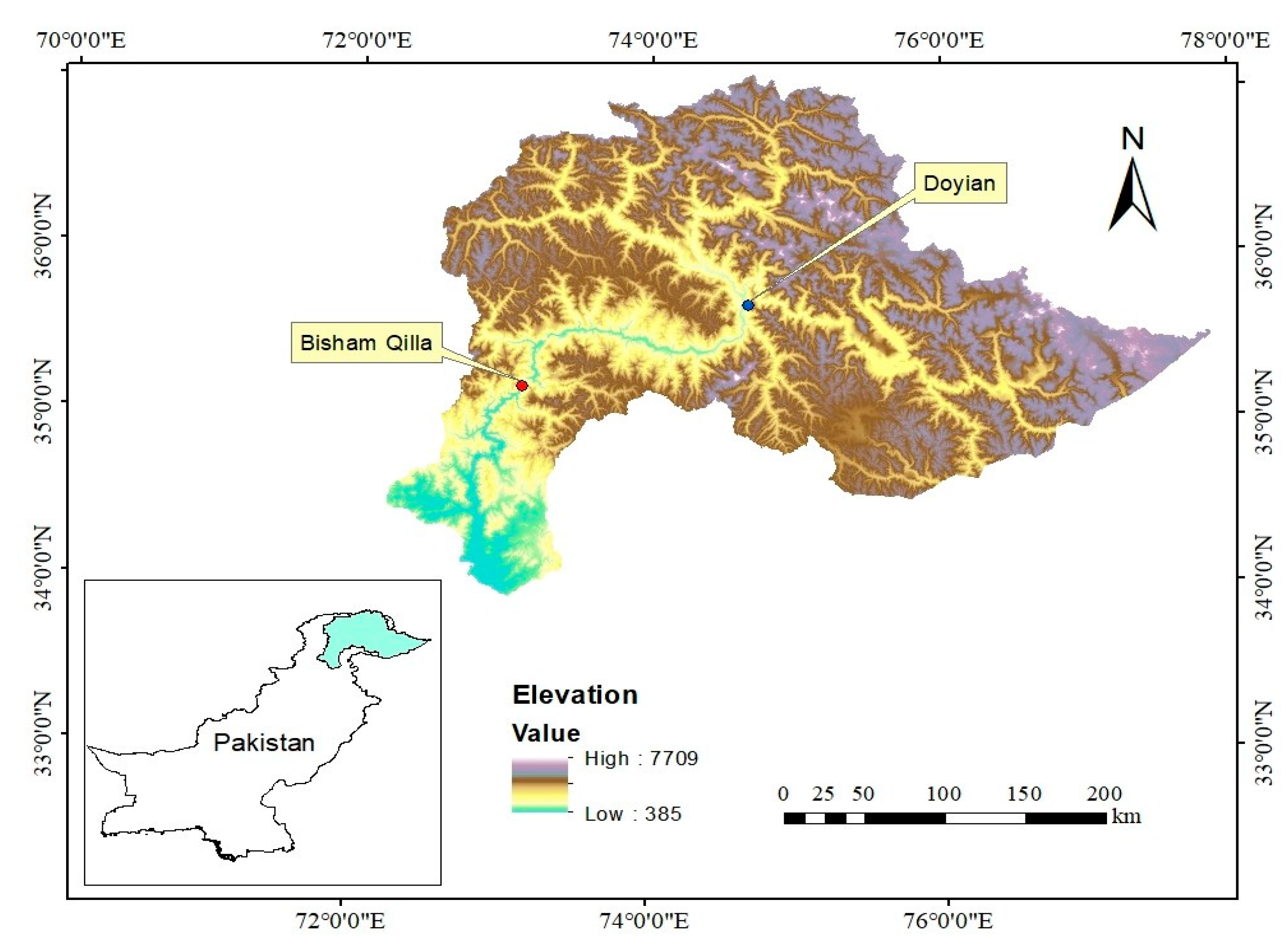
3.1. Description of the Study Area

The Indus River is 2880 km long and the Upper Indus river basin (UIB) is one of the glacierized, mountainous and snow-fed catchment [48]. The UIB, a part of the Indus basin system, situated upstream of Tarbela dam with 1150 km total length, 165,400 km² drainage area and ice reserves of 2174 km³. The elevation in UIB varies from 455 m to 8611 m and the climate fluctuates considerably inside the basin due to variation in altitude [49,50,51]. The average yearly precipitation varies from 100 to 200 mm [52,53]. The detailed description of the study area is given in Figure 3.

3.2. Modeling and Water Quality Dataset

The water quality modeling using AI methods were carried out using four main steps: (1) Data preparation; (2) Model development; (3) Model assessment and validation; and (4) Robustness analysis. The water quality dataset used in this study was obtained from WAPDA, Pakistan. The final data contained 360 monthly data points collected from 1975 to 2005 measured at Doyian and Bisham Qilla outlets. The dataset included nine parameters, namely, calcium (Ca), magnesium (Mg), sodium (Na), chloride (Cl), sulphate (SO₄), pH, bicarbonates (HCO₃), TDS and EC. The statistical parameters of the water quality data are shown in

Table 3. Statistical indicators of the modeling dataset.

Variable	Unit	Range	SD	Mean	Minimum	Maximum	Skewness	Kurtosis
INPUTS
Calcium (Ca)	meq/L	1.80	0.31	1.49	0.65	2.45	0.94	3.01
Magnesium (Mg)	meq/L	2.60	0.33	0.66	0.04	2.64	0.44	0.51
Sodium (Na)	meq/L	8.95	0.67	0.51	0.05	9.0	2.10	3.92
Chloride (Cl)	meq/L	4.15	0.20	0.27	0.05	4.2	1.43	3.15
Sulphate (SO4)	meq/L	3.11	0.34	0.51	0.1	3.2	0.83	0.55
Bicarbonate (HCO3)	meq/L	7.10	0.61	1.82	0.3	7.4	0.76	0.89
PH	-	1.22	0.65	7.83	7.08	8.3	−0.47	0.23
OUTPUTS
TDS	ppm	200	38.64	138.17	60	260	0.86	1.19
EC	µS/cm	358	67.49	244.65	92	450	0.71	0.91

Total number of data points (n) = 360.

. The typical values of TDS in the study area ranges from 60 ppm to 260 ppm, while, the EC values lies between 92 µS/cm to 450 µS/cm. The WHO guidelines suggested the permissible range of TDS in drinking water is 300–600 mg/L, while the allowable limit for agriculture water is 450–2000 mg/L [54,55]. The concentration of both the TDS and EC lies within the permissible limit; however, it is the need of time to measure important water quality indicators accurately with minimum efforts. The correlation matrix between the input parameters and modeling output (TDS and EC) is tabulated in

Table 4. Correlation matrix of TDS (Bold values show the significant correlation with other parameters).

Parameters	Ca	Mg	Na	HCO3	Cl	SO4	PH	TDS
Ca	1
Mg	0.0194	1
Na	−0.0037	0.4712	1
HCO3	0.0363	0.5324	0.7414	1
Cl	0.0239	0.5035	0.7041	0.5296	1
SO4	0.0212	0.5415	0.4853	0.2749	0.3698	1
PH	0.0025	0.0737	0.0415	0.0545	0.0561	−0.0445	1
TDS	0.7452	0.7001	0.8629	0.8176	0.7411	0.6297	0.6210	1

and

Table 5. Correlation matrix of EC (Bold values show the significant correlation with other parameters).

Parameters	Ca	Mg	Na	HCO3	Cl	SO4	PH	EC
Ca	1
Mg	0.0194	1
Na	−0.0037	0.4712	1
HCO3	0.0363	0.5324	0.7414	1
Cl	0.0239	0.5035	0.7041	0.5296	1
SO4	0.0212	0.5415	0.4853	0.2749	0.3698	1
PH	0.0025	0.0737	0.0415	0.0545	0.0561	−0.0445	1
EC	0.7539	0.8632	0.7672	0.8545	0.8951	0.7954	0.6202	1

, respectively. According to available literature, adding too much input parameters that have a weak correlation with the model output adversely affects the performance of the model and increases the complexity and computational time [50]. Keeping in view the water quality dataset and the correlation among inputs and the targeted TDS and EC levels, seven parameters (Ca, Mg, Na, Cl, SO₄, pH, and HCO₃) were selected as significant inputs for GEP, ANN and LRM model development. As a usual practice, the dataset was randomly separated into 70% (252 records) and 30% (108 records) for models training and testing, respectively.

3.3. Models Performance Evaluation

The efficiency of the developed GEP, ANN and LRM models was determined using selected indicators such as Root Mean Squared Error (RMSE), Nash Sutcliff efficiency (NSE), correlation coefficient (R²), and Mean Absolute Error (MAE) [56]. The NSE ranges between negative infinity to 1 with value over 0.65 represents a reasonable estimation [57,58]. The value of R² varies between 0 and 1 [57]. The RMSE and MAE are error type parameters mostly followed in modeling studies. Lesser value of RMSE and MAE are ideal. The mathematical formulae for the aforementioned indicators are illustrated below as Equations (3)–(6), respectively.

$$RMSE=\sqrt{\frac{{{\displaystyle \sum }}_{i=1}^n{(P_i-M_i)}^2}{N}}$$

(3)

$$NSE=1-\frac{{{\displaystyle \sum }}_{i=1}^n{\left(M_i-P_i\right)}^2}{{{\displaystyle \sum }}_{i=1}^n{\left(M_i-{\overline{M}}_i\right)}^2}$$

(4)

$$R^2=\frac{{{\displaystyle \sum }}_{i=1}^n\left(M_i-{\overline{M}}_i\right)(P_i-{\overline{P}}_i)}{\sqrt{{{\displaystyle \sum }}_{i=1}^n{(M_i-{\overline{M}}_i)}^2{{\displaystyle \sum }}_{i=1}^n{(P_i-{\overline{P}}_i)}^2}}$$

(5)

$$MAE=\frac{1}{n}{{\displaystyle \sum }}_{i=1}^n\left|P_i-M_i\right|$$

(6)

where n represents the data points; M_i and P_i are actual and model simulated values, respectively, and ${\overline{M}}_i$. and ${\overline{P}}_i$ are mean actual and model mean simulated values, respectively.

4. Results and Discussion

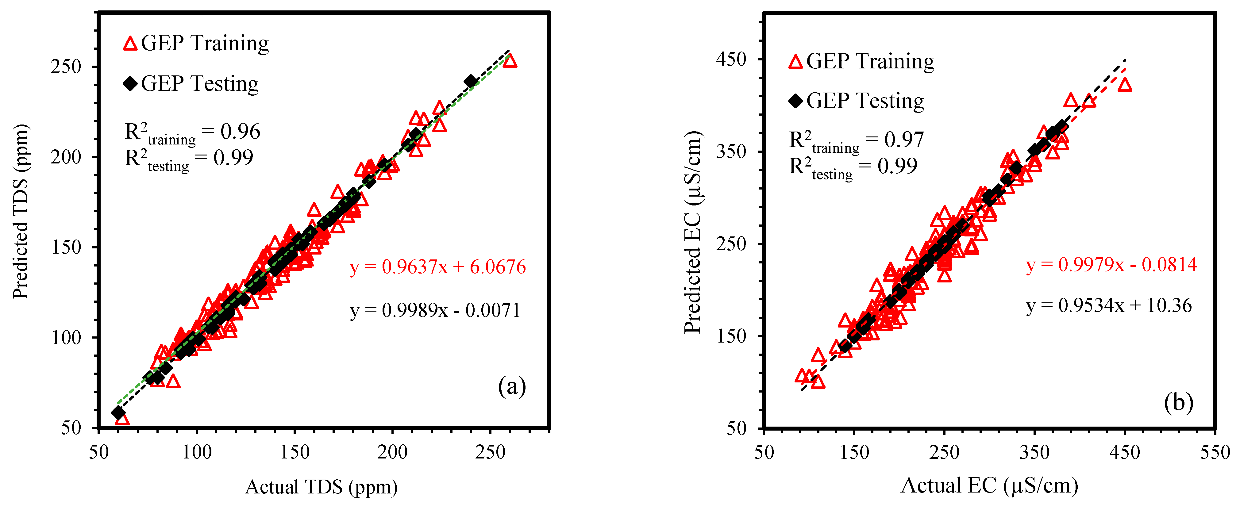
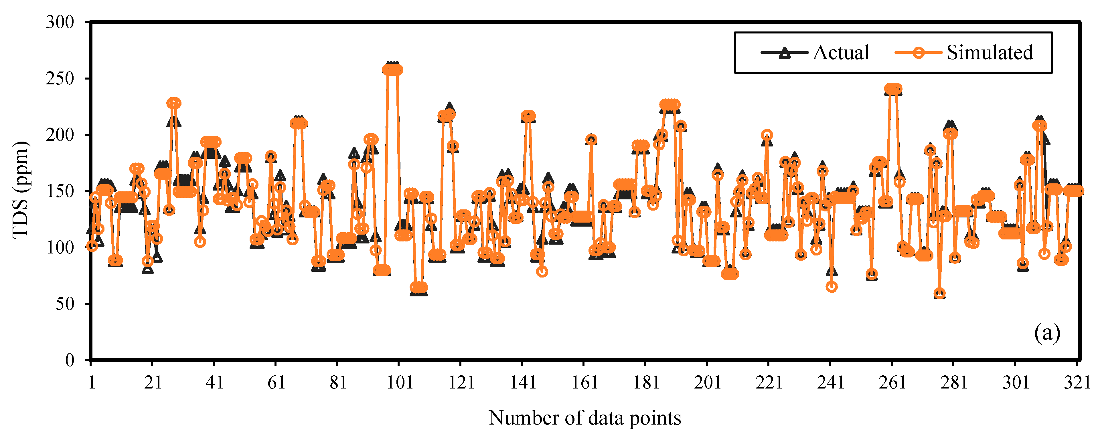
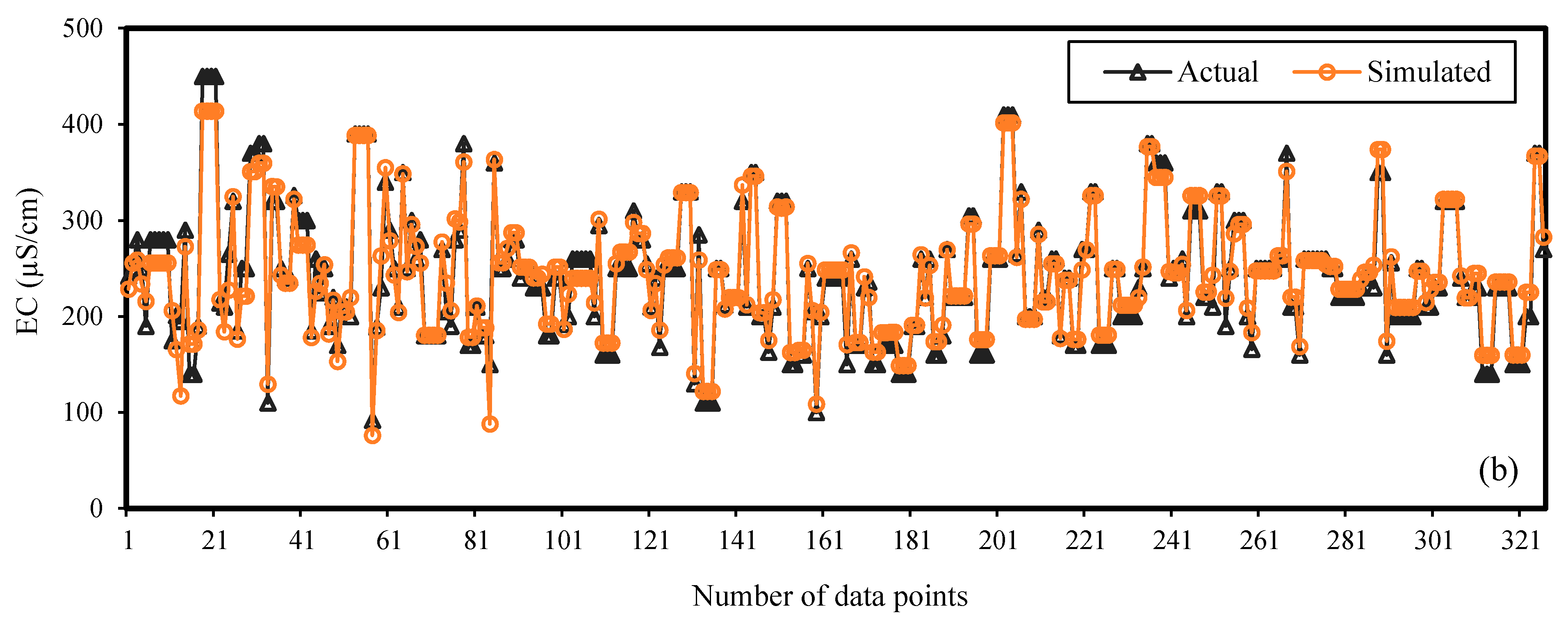
4.1. Formulation of TDS and EC Using GEP

For the GEP model for TDS and EC formulation, the Equations (7) and (8) are developed to forecast the TDS and EC level on monthly basis. These Equations were formulated using seven parameters as significant inputs for GEP model and highlighted its novelty in the accurate prediction of the desired output. Moreover, the modeling results for TDS and EC estimation, as predicted by GEP, are graphically presented in Figure 4 and Figure 5, respectively, for both training and testing.

$$TDS\left(ppm\right)=A+B+C-D$$

(7)

where

$$\begin{array}{c}A=((\frac{20390}{Ca}{)}^{\frac{1}{3}}-22HC{O}_3)\times {\left(S{O}_4-HC{O}_3\right)}^{\frac{1}{3}}\\ B=\frac{1}{HC{O}_3{}^{\frac{1}{3}}\times \ln {\left(8.14Cl-1.11\right)}^2}\\ C=\left(4.15+Na\right)\times 25-Na\times HC{O}_3\\ D=\frac{28}{Ca}\left(Mg\times Cl\times 1.17+\frac{S{O}_4}{1.03}\right)\times \left(51-7.33Cl\right)\end{array}$$

$$EC\left(\mathsf{\mu }S/cm\right)=A+B+C$$

(8)

where

$$\begin{array}{c}A=\left(9.6Cl+5.1S{O}_4-\ln HC{O}_3\right)\times {(4.9-HC{O}_3)}^2\\ B=\left\{\left(S{O}_4\times PH\times 2.6-\frac{32.7}{CA}\right)-5.8\right\}\times HC{O}_3\\ C=\left(Na+HC{O}_3\times 10.4-S{O}_4\times Cl\right)\times 12.12\end{array}$$

It is evident from Figure 4 and Figure 5 that the proposed GEP model had successfully took the effect of all the modeling inputs. The developed GEP model for both TDS and EC was selected after running a set of algorithms. The performance measure indicators of all the models are listed in

Table 6. Summary of statistical results for GEP, ANN, and LRM models.

Output	Model	Training				Testing
		NSE	R2	MAE	RMSE	NSE	R2	MAE	RMSE
TDS	GEP	0.96	0.96	6.58	7.10	0.99	0.99	1.38	1.57
	ANN	0.95	0.94	4.80	6.37	0.85	0.88	5.50	13.1
	LRM	0.97	0.93	5.22	6.69	0.90	0.91	3.83	10.8
EC	GEP	0.96	0.97	12.2	14.4	0.99	0.99	1.51	1.74
	ANN	0.93	0.95	6.67	10.81	0.90	0.90	13.1	13.5
	LRM	0.95	0.92	11.93	16.37	0.94	0.92	11.0	26.70

. Considering the TDS estimated by GEP, the NSE, R², MAE and RMSE were found to be 0.96, 0.96, 6.58, 7.10 for model training data and 0.99, 0.99, 1.38, 1.57 for the testing data, respectively. Similarly, GEP results for EC during model training, the NSE, R², MAE and RMSE were observed to be 0.96, 0.97, 12.2 and 14.4. For EC model testing, the goodness of fit was found to be 0.99, 0.99, 1.51 and 1.74, respectively. According to available literature, the R² value above 0.8 is reasonable [59], while, low MAE, RMSE and higher R² and NSE demonstrate adequate estimation of the model as compared with the actual data [36]. In our study, the R² is above 0.9 for both TDS and EC data, therefore, emphasized the reliable and accurate results of the developed GEP technique.

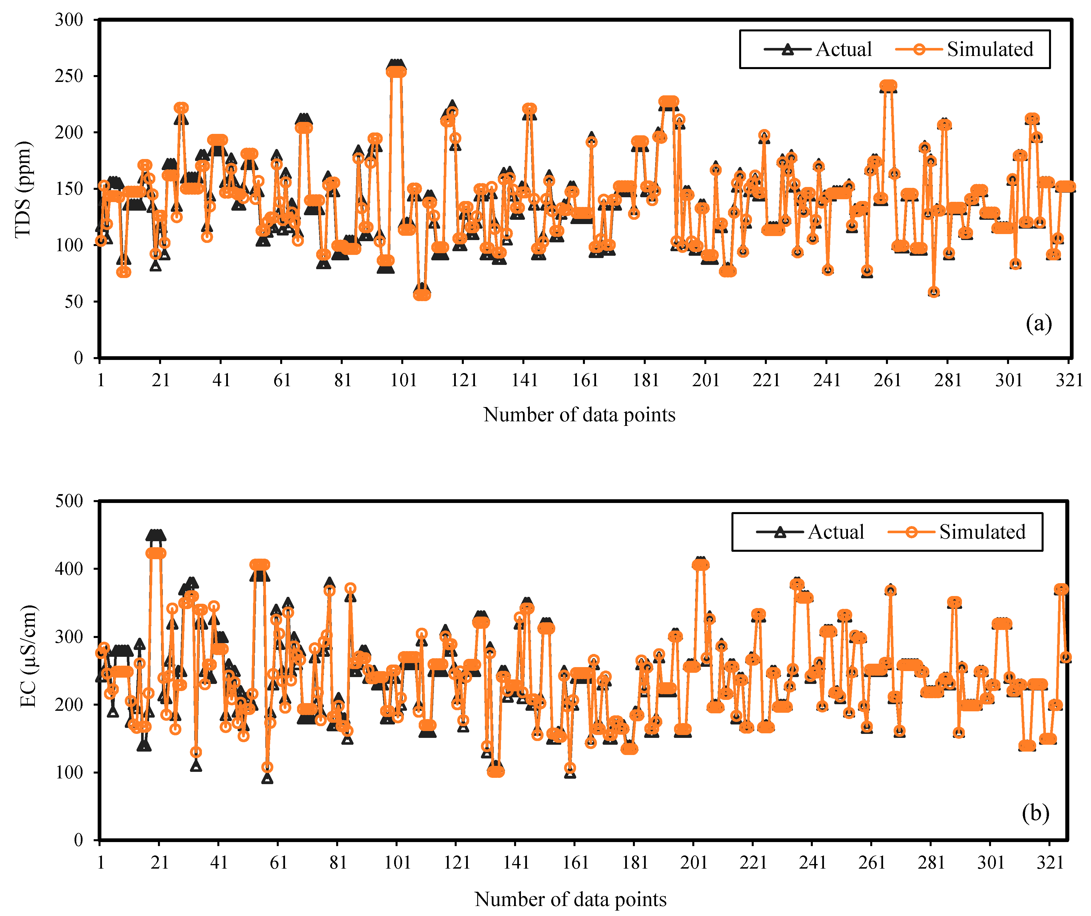
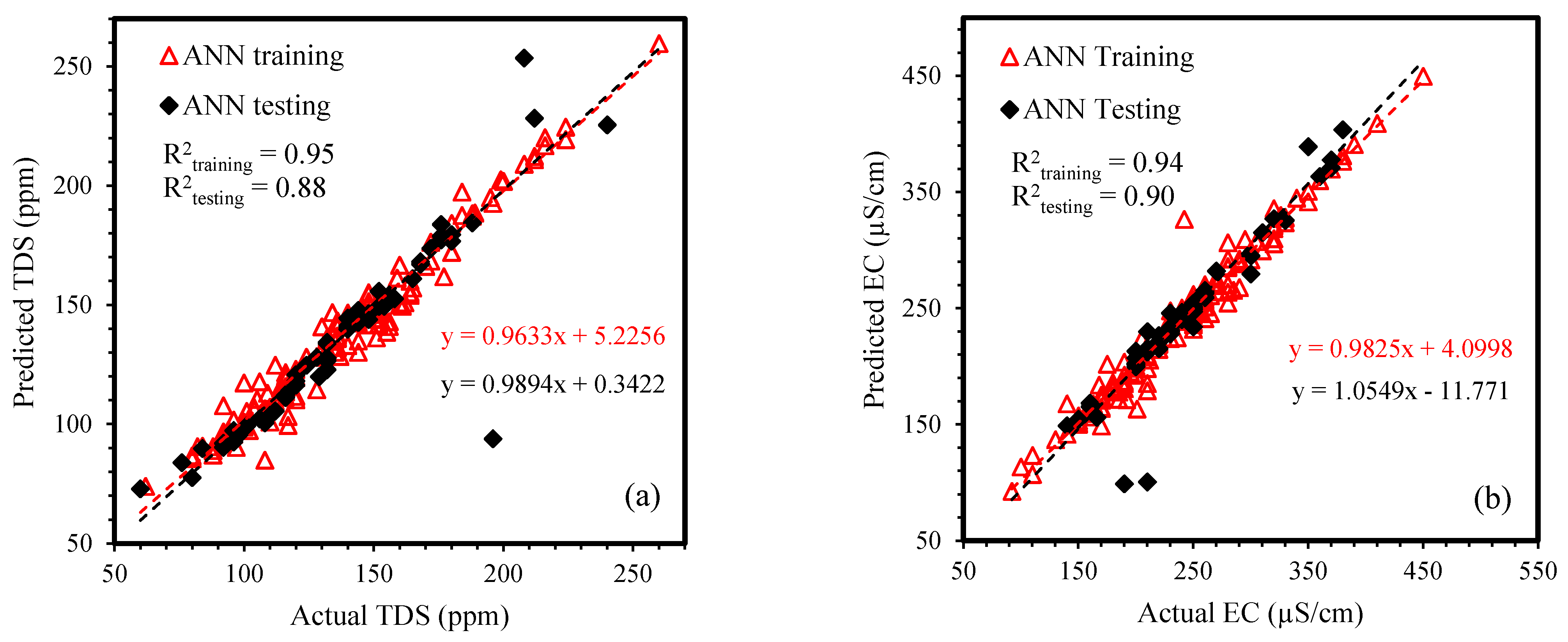
4.2. ANN Modeling Output

Figure 6 and Figure 7 shows the ANN estimated results against the measured data for both TDS and EC data. A trial-and-error method with optimization routine was employed to select the best ANN architecture. During the ANN model training period on TDS data, the values of NSE, R², MAE and RMSE were observed to be 0.95, 0.94, 4.80 and 6.37, respectively. For TDS testing dataset, the values of statistical indicators were found to be 0.85, 0.88, 5.50 and 13.1, respectively.

Similarly, the ANN model performance for training data in EC prediction was assessed by mean of statistical measures. The statistical variables (NSE, R², MAE and RMSE) were found to be 0.93, 0.95, 6.67 and 10.81, respectively for training data and 0.90, 0.90, 13.1 and 13.5 for EC testing data. The ANN modeling outcome (in term of R²) indicated that the performance of the ANN on training dataset is accurate than on the testing data. The values of NSE and R² decreased and RMSE increased for the testing data. This may be considered as one of the drawbacks of the ANN model and can be attributed to the black box nature and inexplicable behavior of ANN, in comparison with other modeling techniques.

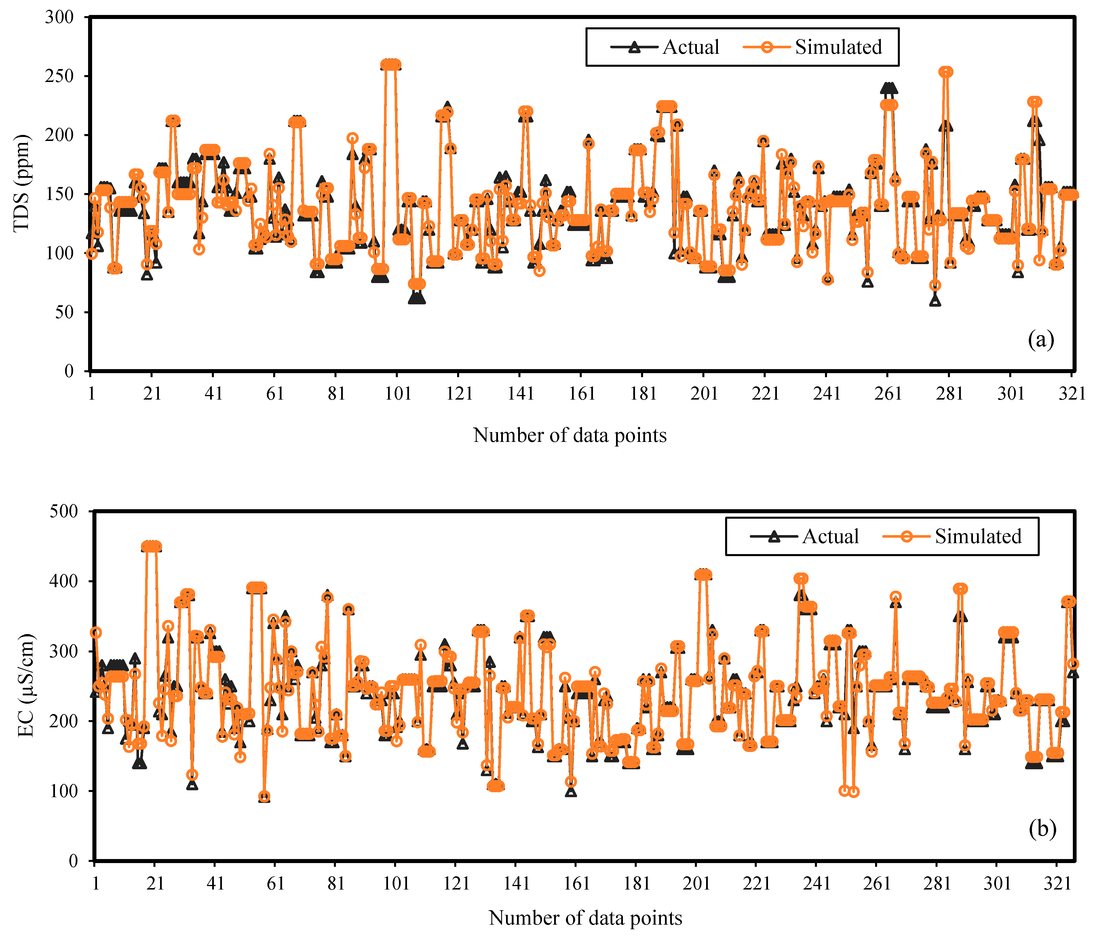
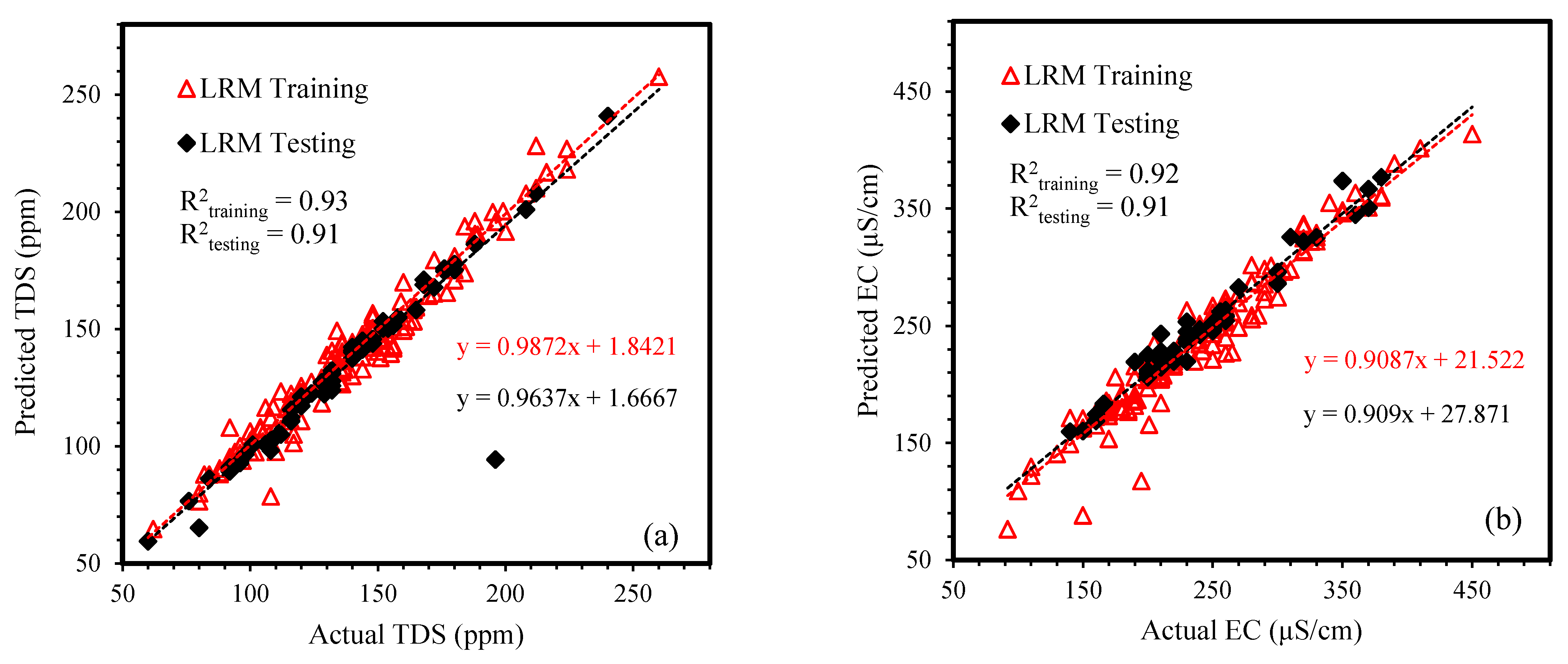
4.3. Linear Regression Modeling for TDS and EC

The results for linear regression model (LRM) are presented in Figure 8 and Figure 9 for both TDS and EC with a satisfactorily estimated output. For LRM, the NSE and R² values were found to be 0.97 and 0.93 for training data and 0.90 and 0.91 for testing dataset, respectively, in modeling the TDS. Similarly, the EC modeling output estimated by LRM, the NSE and R² were equal to 0.95 and 0.92 for model training data and 0.94 and 0.92 for model testing data, respectively. The LRM results shows the declining accuracy (in term of statistical indicators) during the model testing phase which is one of the main drawback of regression-based modeling techniques [50].

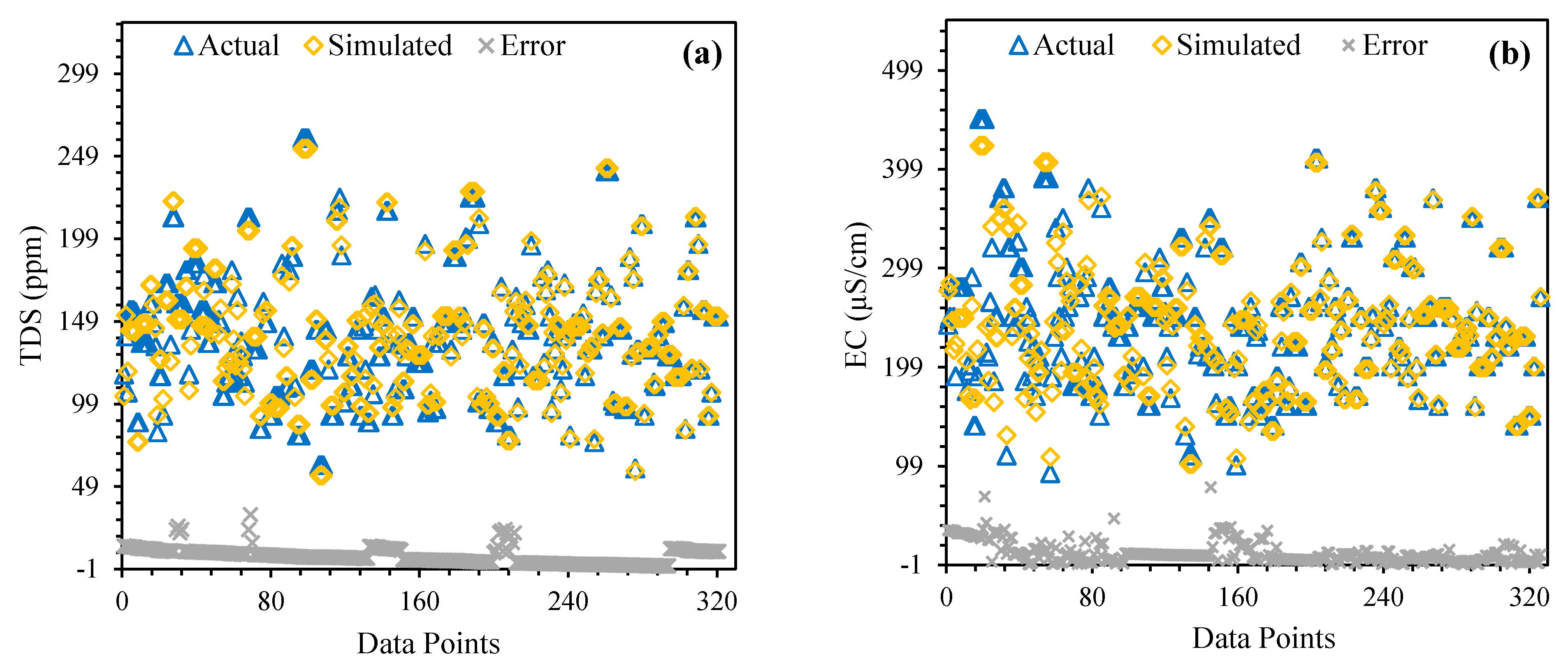
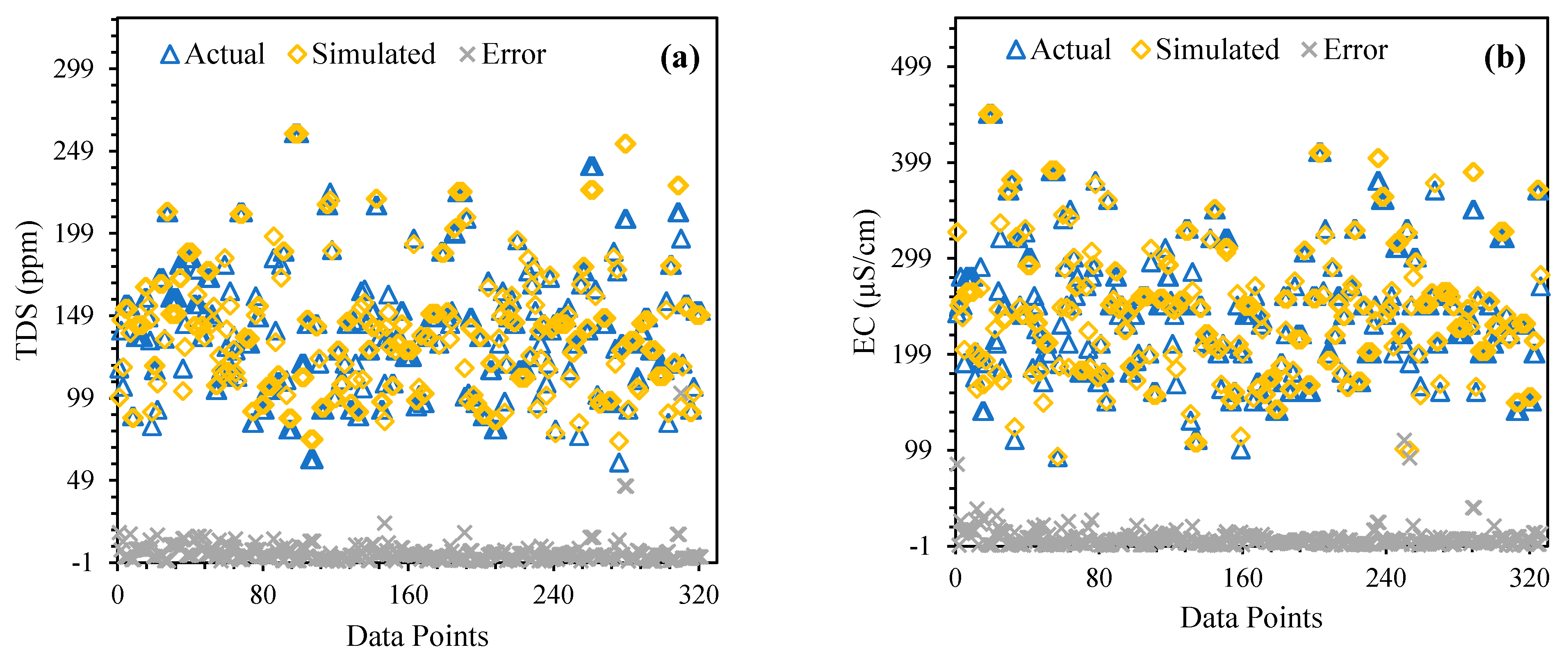
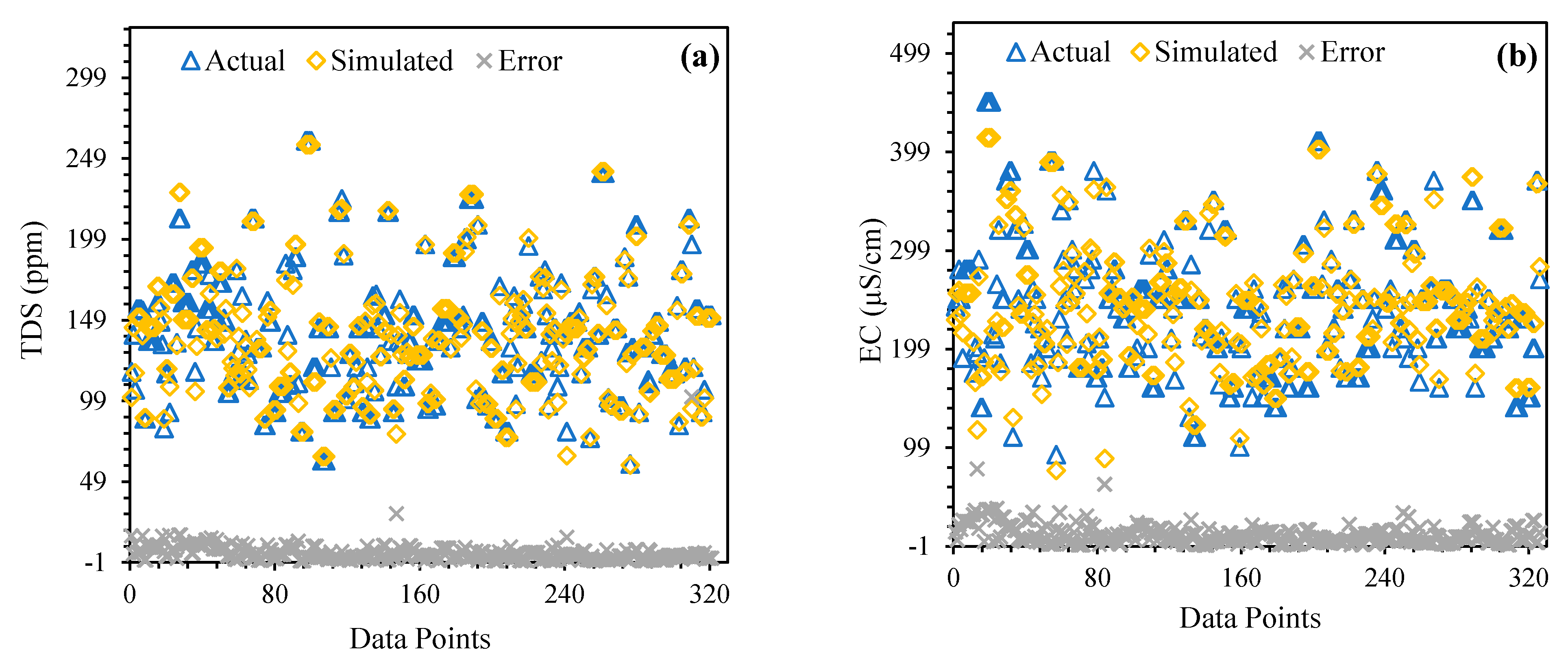
4.4. Models Comparative Analysis and Error Assessment

The output of all the developed models is compared to draw a comparative analysis pertaining to the prediction capability of AI and regression techniques. Considering the performance of the GEP technique, it outclasses other models (ANN and LRM) during training as well as testing phase and remained the accurate one. The lowest RMSE values was also attained by GEP which highlighted its overall supremacy. Keeping in view the performance of the ANN model, it showed good prediction capability during training but its performance reduced on testing dataset. The declined performance may be considered a limitation of the ANN model and can be attributed to the inexplicable behavior and the difficulty in the network structure of ANN [26,27]. As far as the performance of LRM is concerned, behavior (reduced performance during model training) similar to ANN was observed. The results of the observed and LRM simulated data tend to deviate largely as compared to GEP and ANN, which exposed the overall enhanced prediction capacity of AI based modeling techniques. The comparative performance indicators of the models are listed in Table 6.

The average absolute error between the model simulated and actual data are graphically illustrated in Figure 10, Figure 11 and Figure 12 for GEP, ANN and LRM models, respectively. For GEP, the mean absolute error was 2.3 ppm and 3.01 μS/cm in predicting TDS and EC levels, respectively. The maximum and minimum error in GEP predicted results for TDS (3.3 ppm and 0.23 ppm) and EC (2.9 μS/cm and 0.4 μS/cm) was observed. The error graphs between the simulated and actual data are illustrated in Figure 11a,b for ANN. The average respective absolute error was observed to be 5.3 ppm and 6.9 μS/cm for TDS and EC modeling simulated by ANN. Lastly, Figure 12a,b demonstrated the average error values predicted by LRM. The mean absolute error for TDS and EC data was found to be 8.9 ppm and 10.5 μS/cm, respectively, predicted by LRM. The result shows the accurate performance, reduced error and high correlation of GEP model as compared with other developed techniques (ANN and LRM). Conclusively, the performance of the models follows the order of GEP > ANN > LRM in predicting both the TDS and EC.

4.5. Models External Validation

The effectiveness of a model significantly depends on input data [11]. In order to check the correctness of a dataset for establishing a linkage among variables, Frank and Todeschini [60] suggested that five should be the ratio between data points and input variables. In our study, the aforementioned ratio is 36.0 (252/7) and 18.0 (108/6) for train and test data, respectively, which satisfies the requirement of dataset selection. Golbraikh and Tropsha [61] recommended that slope of line passing through the origin must be close to unity. Roy (2008) [62] presented an indicator (R_m) and suggested that value of R_m should be above 0.5. Alavi et al. (2011) [63] proposed that R_o² and R_o’² among actual and projected values must be nearly 1. In our study, the performance of the adopted techniques (GEP, ANN and LRM) was assessed by the aforementioned criteria and the results are summarized in

Table 7. Statistical indicators for external validation of GEP, ANN and LRM models.

S. No.	Equation	Criteria	Technique	Value	Suggested by
1	$R=\frac{{{\displaystyle \sum }}_{i=1}^n\left(M_i-{\overline{M}}_i\right)(P_i-{\overline{P}}_i)}{\sqrt{{{\displaystyle \sum }}_{i=1}^n{(M_i-{\overline{M}}_i)}^2{{\displaystyle \sum }}_{i=1}^n{(P_i-{\overline{P}}_i)}^2}}$	R > 0.8	GEP	0.96	[60]
			ANN	0.98
			LRM	0.97
2	$k=\frac{{{\displaystyle \sum }}_{i=1}^n(M_i-P_i)}{M_i{}^2}$	0.85 < k < 1.15	GEP	1.004	[61]
			ANN	0.997
			L	0.992
3	$k^{\prime }=\frac{{{\displaystyle \sum }}_{i=1}^n(M_i-P_i)}{P_i{}^2}$	0.85 < k′ < 1.15	GEP	0.995	[61]
			ANN	1.002
			LRM	1.007
4	$\begin{array}{l}{R}_m=R^2\times (1-\sqrt{\left|R^2-R_0{}^2\right|}\\ R_0{}^2=\frac{{{\displaystyle \sum }}_{i=1}^n{\left(P_i-M_i{}^0\right)}^2}{{{\displaystyle \sum }}_{i=1}^n{(P_i-\overline{P_i{}^0})}^2},M_i{}^0=k\times P_i\\ \acute{R_0{}^2}=\frac{{{\displaystyle \sum }}_{i=1}^n{\left(M_i-P_i{}^0\right)}^2}{{{\displaystyle \sum }}_{i=1}^n{(M_i-\overline{M_i{}^0})}^2},P_i{}^0=k^{\prime }\times M_i\end{array}$	Rm > 0.5	GEP	0.799	[62]
			ANN	0.820
			LRM	0.811
		$R_0{}^2\cong 1$	GEP	0.999
			ANN	0.999
			LRM	099
		$\acute{R_0{}^2}\cong 1$	GEP	0.999
			ANN	0.999
			LRM	999

.

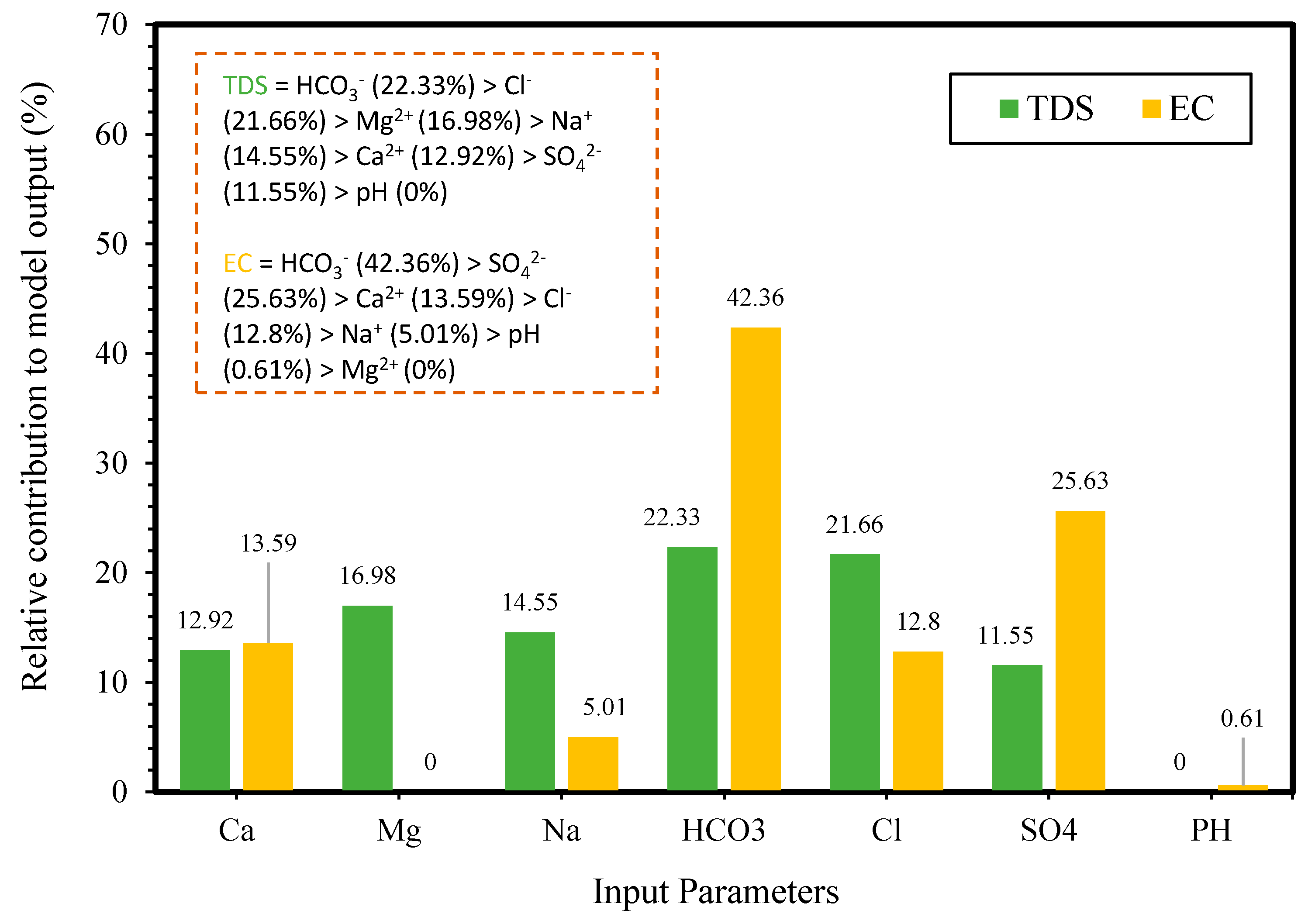
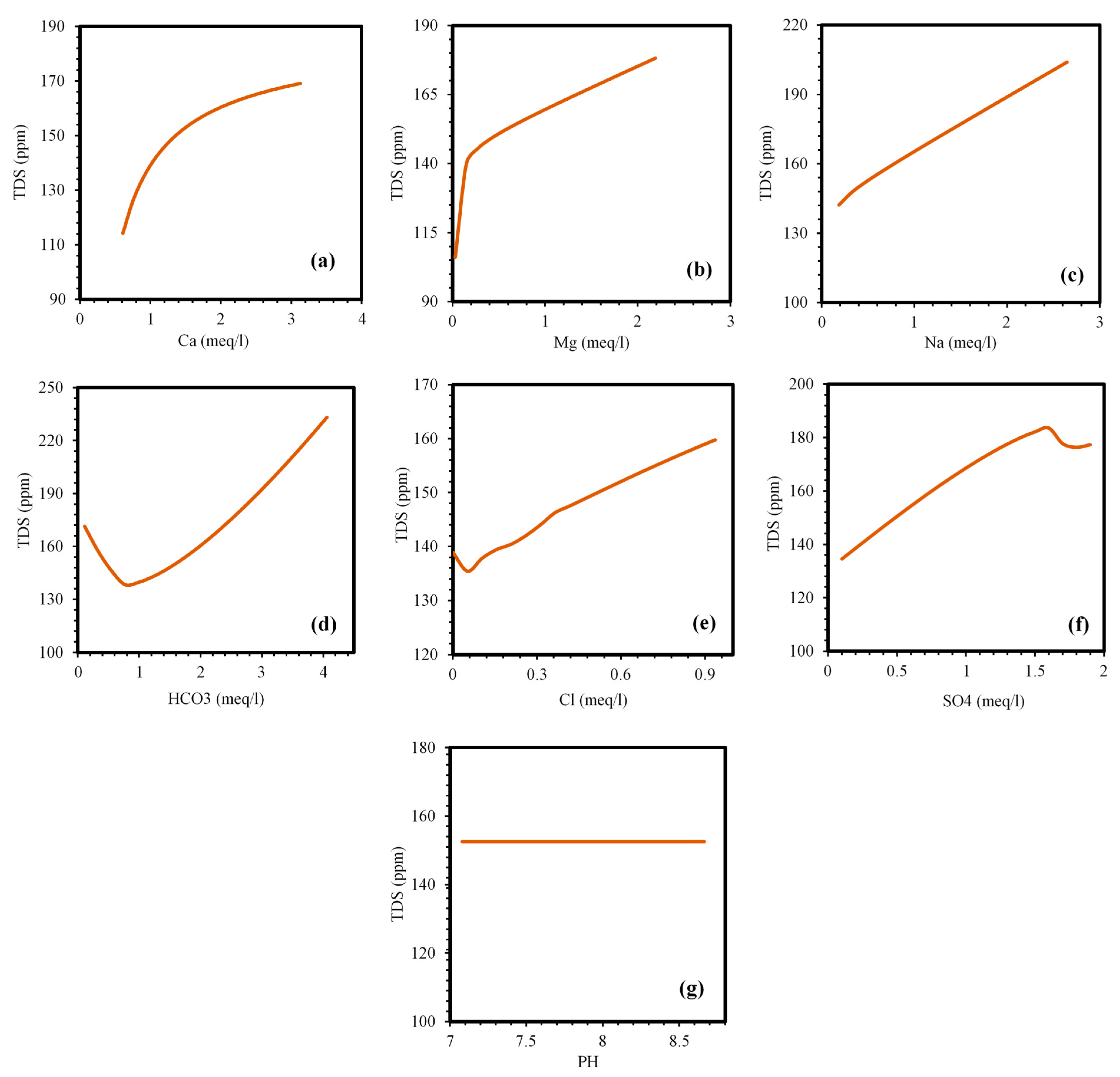
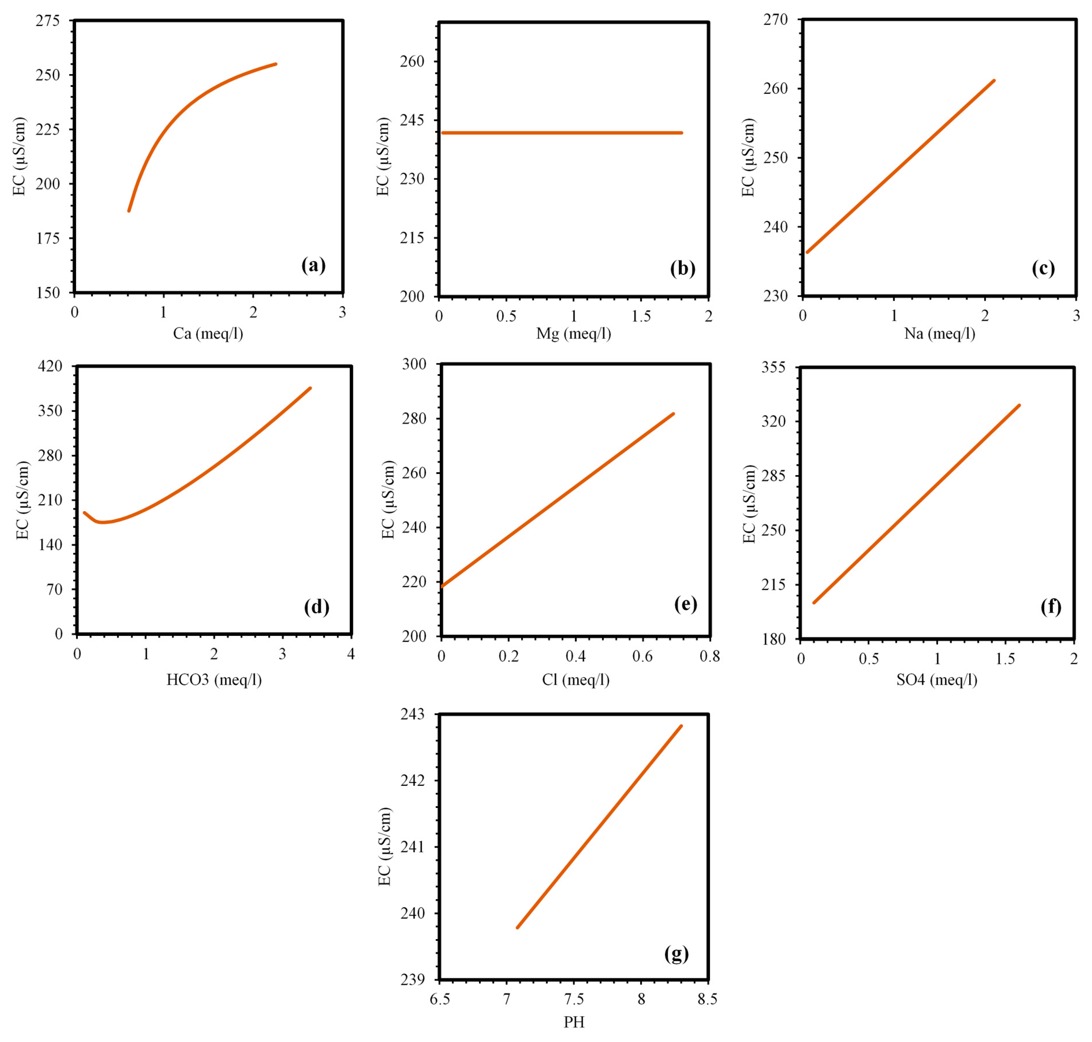
4.6. Sensitivity and Parametric Study

In AI modeling, it is important to carry out some analysis and checks to confirm the accuracy of the models. A reliable performance of a model on training and testing dataset does not guarantee the generalized accuracy and robustness. To find out the effective parameters and ensure that the model has incorporated the effect of all the inputs, the sensitivity and parametric analysis has been proposed in literature [39,50]. For a known dataset and input parameters, a model could provide a desirable outcome but it is not certain to provide the same accuracy for unknown data. Though, it is obligatory to carry out the sensitivity and parametric study to determine the involvement of inputs for predicting output. In the present research, the techniques proposed by Gandomi et al. (2013) [64] was used. The researchers developed the Equations (9) and (10) for finding out the effect and sensitivity of input variables on the modeling output.

$$N_i=f_{max}\left(x_i\right)-f_{min}\left(x_i\right)$$

(9)

$$S_i=\frac{N_i}{{{\displaystyle \sum }}_{j=i}^n{N}_j}\times 100$$

(10)

The $f_{max}\left(x_i\right)$ and $-f_{min}\left(x_i\right)$ are the maximum and minimum of the estimated output over the ith output.

Various sensitive parameters were identified effecting the targeted output and the results are illustrated in Figure 13 for both TDS and EC output. The graphs indicated that bicarbonates (HCO₃) is the most significant parameter with 22.3% and 42.3% relative contribution to TDS and EC concentration, respectively. Similarly, the second influencing parameter is Cl for TDS and SO₄ for EC with 21.6% and 25.6% respective contribution. The results further demonstrated that the targeted output (TDS and EC) is likely to be least effected by pH. Moreover, Mg is contributing 16.98% to TDS and almost 0% to EC (least significant for EC).

Parametric analysis was performed by keeping all the variables constant at their mean values and changing a single parameter at a time. Figure 14 and Figure 15 graphically demonstrate the respective prediction capacity of the proposed techniques for TDS and EC modeling with a variation in the input parameters. The output of the parametric study exposed that the concentration of TDS and EC follows an increasing tendency with a variation in each input except for PH (where its concentration is constant). According to available literature, both the outputs (TDS and EC) are associated with the salts/ions, and consequently, a fluctuation in the concentration of ions affect the TDS and EC level [55]. The same trend was observed in our study, because most of the input parameters are inorganic and organic salts. Hence the increasing trend of TDS and EC with a variation in model input parameters may be attributed to the salty concentration in surface water. Only one parameter (Mg) remained the least significant one, which did not have a momentous effect on EC level as compared to other modeling inputs.

4.7. Environmental Aspects of Water Quality Modeling

The AI-based models are very useful tools in predicting the concentration, distribution and risk of chemical pollutants in a given surface water body. The modeling outcome from these models are crucial for environmental impact assessment and might provide a supportive technique to environmental management agencies for decision making pertaining to rising water pollution [8]. Moreover, models are helpful in providing objective means of processing the complex information related to water quality condition. In this study, the predictive capacity of the well-known GEP, ANN and LRM models was assessed in predicting the TDS and EC concentration in a highly glacierized and mountainous catchment, the Upper Indus River Basin (UIB). UIB is a major source of contributing water to downstream areas where the water is used for drinking as well as agricultural production. The direct and in-situ measurement of water quality parameters is almost impossible in such a complicated watershed. Therefore, the use of modeling technique is indispensable to provide a deep insight regarding the water pollution. Furthermore, the GEP model provides mathematical expressions which will be very helpful for government organizations and environmental pollution control agencies in accessing the condition of water by using minimum number of input parameters.

5. Conclusions

The present study was mainly dedicated in applying AI and regression methods for EC and TDS prediction in the expanded part of the glacierized and mountainous catchment i.e., upper Indus river basin. The dataset, acquired from both Doyian and Bisham Qilla outlets, was utilized for the models’ development. Secondly, the accuracies of the artificial neural network (ANN), gene expression programming (GEP) and linear regression model (LRM) were compared and a robustness analysis was performed to determine the most reliable model. Regardless of several factors that have influence on water quality, the models were effectively developed utilizing monthly TDS and EC data measured historically. The modeling outcome for the resolved overfitting issue and generalized results was confirmed by external criteria. The sensitivity and parametric analyses were carried out to ensure a robust relation between inputs and desired output. An excellent correlation exhibited among actual and model simulated results for both training and testing data. The performance of the GEP turned out to be the most accurate followed by ANN technique. Both GEP and ANN have the capability to model water quality parameters for a given set of inputs. The GEP mathematical expressions for TDS and EC level could be easily used in predicting monthly TDS and EC. The GEP evaluates suitable association mandatory for representation of the physical processes. The accuracy of the ANN model decreased on testing data and may be attributed to the difficult network structure of ANN. Conclusively, the outcome of the present study will be helpful in assessing the performance of AI models using big dataset for water quality prediction. Moreover, the modeling techniques applied in this study could assist the water quality managers and engineers in developing an effective strategy for successful management of surface water bodies.

References

1. Al-Mukhtar, M.; Al-Yaseen, F. Modeling water quality parameters using data-driven models, a case study Abu-Ziriq marsh in south of Iraq. Hydrology 2019, 6, 24. [Google Scholar] [CrossRef] [Green Version]
2. Li, K.; Wang, L.; Li, Z.; Xie, Y.; Wang, X.; Fang, Q. Exploring the spatial-seasonal dynamics of water quality, submerged aquatic plants and their influencing factors in different areas of a lake. Water 2017, 9, 707. [Google Scholar] [CrossRef] [Green Version]
3. Singh, K.P.; Malik, A.; Mohan, D.; Sinha, S. Multivariate statistical techniques for the evaluation of spatial and temporal variations in water quality of Gomti River (India)—A case study. Water Res. 2004, 38, 3980–3992. [Google Scholar] [CrossRef] [PubMed]
4. Mohammadpour, R.; Shaharuddin, S.; Zakaria, N.A.; Ghani, A.A.; Vakili, M.; Chan, N.W. Prediction of water quality index in free surface constructed wetlands. Environ. Earth Sci. 2016, 75, 139. [Google Scholar] [CrossRef]
5. Schleiter, I.M.; Borchardt, D.; Wagner, R.; Dapper, T.; Schmidt, K.-D.; Schmidt, H.-H.; Werner, H. Modelling water quality, bioindication and population dynamics in lotic ecosystems using neural networks. Ecol. Model. 1999, 120, 271–286. [Google Scholar] [CrossRef]
6. Salami, E.S.; Salari, M.; Ehteshami, M.; Bidokhti, N.T.; Ghadimi, H. Application of artificial neural networks and mathematical modeling for the prediction of water quality variables (case study: Southwest of Iran). Desalin. Water Treat. 2016, 57, 27073–27084. [Google Scholar] [CrossRef]
7. Najah, A.; El-Shafie, A.; Karim, O.A.; El-Shafie, A.H. Application of artificial neural networks for water quality prediction. Neural Comput. Appl. 2013, 22, 187–201. [Google Scholar] [CrossRef]
8. Shah, M.I.; Abunama, T.; Javed, M.F.; Bux, F.; Aldrees, A.; Tariq, M.A.U.R.; Mosavi, A. Modeling surface water quality using the adaptive neuro-fuzzy inference system aided by input optimization. Sustainability 2021, 13, 4576. [Google Scholar] [CrossRef]
9. Sattari, M.T.; Joudi, A.R.; Kusiak, A. Estimation of water quality parameters with data-driven model. J. Am. Water Works Assoc. 2016, 108, E232–E239. [Google Scholar] [CrossRef] [Green Version]
10. Basant, N.; Gupta, S.; Malik, A.; Singh, K.P. Linear and nonlinear modeling for simultaneous prediction of dissolved oxygen and biochemical oxygen demand of the surface water—A case study. Chemom. Intell. Lab. Syst. 2010, 104, 172–180. [Google Scholar] [CrossRef]
11. Gholampour, A.; Gandomi, A.H.; Ozbakkaloglu, T. New formulations for mechanical properties of recycled aggregate concrete using gene expression programming. Const. Build. Mater. 2017, 130, 122–145. [Google Scholar] [CrossRef]
12. Vats, S.; Sagar, B.B.; Singh, K.; Ahmadian, A.; Pansera, B.A. Performance evaluation of an independent time optimized infrastructure for big data analytics that maintains symmetry. Symmetry 2020, 12, 1274. [Google Scholar] [CrossRef]
13. Pakdaman, M.; Falamarzi, Y.; Yazdi, H.S.; Ahmadian, A.; Salahshour, S.; Ferrara, F. A kernel least mean square algorithm for fuzzy differential equations and its application in earth’s energy balance model and climate. Alex. Eng. J. 2020, 59, 2803–2810. [Google Scholar] [CrossRef]
14. Sarkar, A.; Pandey, P. River water quality modelling using artificial neural network technique. Aquat. Procedia 2015, 4, 1070–1077. [Google Scholar] [CrossRef]
15. Chebud, Y.; Naja, G.M.; Rivero, R.G.; Melesse, A.M. Water quality monitoring using remote sensing and an artificial neural network. Water Air Soil Pollut. 2012, 223, 4875–4887. [Google Scholar] [CrossRef]
16. Palani, S.; Liong, S.-Y.; Tkalich, P. An ANN application for water quality forecasting. Mar. Pollut. Bullet. 2008, 56, 1586–1597. [Google Scholar] [CrossRef]
17. Firat, M.; Güngör, M. Monthly total sediment forecasting using adaptive neuro fuzzy inference system. Stoch. Environ. Res. Risk Assess. 2010, 24, 259–270. [Google Scholar] [CrossRef]
18. Chen, L.; Jamal, M.; Tan, C.; Alabbadi, B. A study of applying genetic algorithm to predict reservoir water quality. Int. J. Model. Optim. 2017, 7, 98. [Google Scholar] [CrossRef] [Green Version]
19. Martí, P.; Shiri, J.; Duran-Ros, M.; Arbat, G.; De Cartagena, F.R.; Puig-Bargués, J. Artificial neural networks vs. gene expression programming for estimating outlet dissolved oxygen in micro-irrigation sand filters fed with effluents. Comput. Electron. Agric. 2013, 99, 176–185. [Google Scholar] [CrossRef]
20. Amin, R.; Shah, K.; Khan, I.; Asif, M.; Salimi, M.; Ahmadian, A. Efficient numerical scheme for the solution of tenth order boundary value problems by the Haar wavelet method. Mathematics 2020, 8, 1874. [Google Scholar] [CrossRef]
21. Farooq, F.; Nasir Amin, M.; Khan, K.; Rehan Sadiq, M.; Faisal Javed, M.; Aslam, F.; Alyousef, R.A. Comparative study of random forest and genetic engineering programming for the prediction of compressive strength of high strength concrete (HSC). Appl. Sci. 2020, 10, 7330. [Google Scholar] [CrossRef]
22. Aslam, F.; Farooq, F.; Amin, M.N.; Khan, K.; Waheed, A.; Akbar, A.; Alabdulijabbar, H. Applications of gene expression programming for estimating compressive strength of high-strength concrete. Adv. Civ. Eng. 2020, 2020, 1–23. [Google Scholar] [CrossRef]
23. Shah, M.I.; Amin, M.N.; Khan, K.; Niazi, M.S.K.; Aslam, F.; Alyousef, R.; Mosavi, A. Performance evaluation of soft computing for modeling the strength properties of waste substitute green concrete. Sustainability 2021, 13, 2867. [Google Scholar] [CrossRef]
24. Shah, M.I.; Memon, S.A.; Khan Niazi, M.S.; Amin, M.N.; Aslam, F.; Javed, M.F. Machine learning-based modeling with optimization algorithm for predicting mechanical properties of sustainable concrete. Adv. Civ. Eng. 2021, 2021. [Google Scholar] [CrossRef]
25. Haykin, S. Neural Networks: A Comprehensive Foundation; Prentice-Hall, Inc.: Upper Saddle River, NJ, USA, 1999; Volume 7458, pp. 161–175. [Google Scholar]
26. Tung, T.M.; Yaseen, Z.M. A survey on river water quality modelling using artificial intelligence models: 2000–2020. J. Hydrol. 2020, 585, 124670. [Google Scholar]
27. Bermejo, J.F.; Fernández, J.F.G.; Polo, F.O.; Márquez, A.C. A review of the use of artificial neural network models for energy and reliability prediction. A study of the solar PV, hydraulic and wind energy sources. Appl. Sci. 2019, 9, 1844. [Google Scholar] [CrossRef] [Green Version]
28. Koza, J.R.; Koza, J.R. Genetic Programming: On the Programming of Computers by Means of Natural Selection; MIT Press: Cambridge, MA, USA, 1992; Volume 1. [Google Scholar]
29. Javed, M.F.; Farooq, F.; Memon, S.A.; Akbar, A.; Khan, M.A.; Aslam, F.; Rehman, S.K.U. New prediction model for the ultimate axial capacity of concrete-filled steel tubes: An evolutionary approach. Crystals 2020, 10, 741. [Google Scholar] [CrossRef]
30. Hada, D.S.; Gupta, U.; Sharma, S.C. Seasonal evaluation of hydro-geochemical parameters using goal programming with multiple nonlinear regression. Gen. Math. Notes 2014, 25, 137–147. [Google Scholar]
31. Ahmed, A.N.; Othman, F.B.; Afan, H.A.; Ibrahim, R.K.; Fai, C.M.; Hossain, M.S.; Elshafie, A. Machine learning methods for better water quality prediction. J. Hydrol. 2019, 578, 124084. [Google Scholar] [CrossRef]
32. Granata, F.; Papirio, S.; Esposito, G.; Gargano, R.; De Marinis, G. Machine learning algorithms for the forecasting of wastewater quality indicators. Water 2017, 9, 105. [Google Scholar] [CrossRef] [Green Version]
33. Haghiabi, A.H.; Nasrolahi, A.H.; Parsaie, A. Water quality prediction using machine learning methods. Water Qual. Res. J. 2018, 53, 3–13. [Google Scholar] [CrossRef]
34. Zhang, Y.; Gao, X.; Smith, K.; Inial, G.; Liu, S.; Conil, L.B.; Pan, B. Integrating water quality and operation into prediction of water production in drinking water treatment plants by genetic algorithm enhanced artificial neural network. Water Res. 2019, 164, 114888. [Google Scholar] [CrossRef]
35. Ferreira, C. Gene expression programming: A new adaptive algorithm for solving problems. arXiv 2001, arXiv:cs/0102027. Available online: https://arxiv.org/abs/cs/0102027 (accessed on 5 April 2021).
36. Azim, I.; Yang, J.; Javed, M.F.; Iqbal, M.F.; Mahmood, Z.; Wang, F.; Liu, Q.F. Prediction model for compressive arch action capacity of RC frame structures under column removal scenario using gene expression programming. Structures 2020, 25, 212–228. [Google Scholar] [CrossRef]
37. Lopes, H.S.; Weinert, W.R. A gene expression programming system for time series modeling. In Proceedings of the XXV Iberian Latin American Congress on Computational Methods in Engineering, Recife, Brazil, 10–12 November 2004. [Google Scholar]
38. Shah, M.I.; Javed, M.F.; Alqahtani, A.; Aldrees, A. Environmental assessment based surface water quality prediction using hyper-parameter optimized machine learning models based on consistent big data. Process Saf. Environ. Prot. 2021, 151, 324–340. [Google Scholar] [CrossRef]
39. Iqbal, M.F.; Liu, Q.-F.; Azim, I.; Zhu, X.; Yang, J.; Javed, M.F.; Rauf, M. Prediction of mechanical properties of green concrete incorporating waste foundry sand based on gene expression programming. J. Hazard. Mater. 2020, 384, 121322. [Google Scholar] [CrossRef] [PubMed]
40. Guven, A.; Gunal, M. Genetic programming approach for prediction of local scour downstream of hydraulic structures. J. Irrig. Drain. Eng. 2008, 134, 241–249. [Google Scholar] [CrossRef]
41. Ferreira, C. Gene expression programming in problem solving. In Soft Computing and Industry; Springer: London, UK, 2002; pp. 635–653. [Google Scholar]
42. McCulloch, W.S.; Pitts, W. A logical calculus of the ideas immanent in nervous activity. Bull. Math. Biol. 1943, 5, 115–133. [Google Scholar] [CrossRef]
43. Rumelhart, D.E.; Hinton, G.E.; Williams, R.J. Learning representations by back-propagating errors. Nature 1986, 323, 533–536. [Google Scholar] [CrossRef]
44. Azamathulla, H.M.; Rathnayake, U.; Shatnawi, A. Gene expression programming and artificial neural network to estimate atmospheric temperature in Tabuk, Saudi Arabia. Appl. Water Sci. 2018, 8, 184. [Google Scholar] [CrossRef] [Green Version]
45. Weisberg, S. Applied Linear Regression; John Wiley & Sons: Hoboken, NJ, USA, 2005; Volume 528. [Google Scholar]
46. Montgomery, D.C.; Peck, E.A.; Vining, G.G. Introduction to Linear Regression Analysis; Wiley: New York, NY, USA, 2001. [Google Scholar]
47. Shah, M.I.; Khan, A.; Akbar, T.A.; Hassan, Q.K.; Khan, A.J.; Dewan, A. Predicting hydrologic responses to climate changes in highly glacierized and mountainous region Upper Indus Basin. R. Soc. Open Sci. 2020, 7, 191957. [Google Scholar] [CrossRef] [PubMed]
48. Javed, M.F.; Amin, M.N.; Shah, M.I.; Khan, K.; Iftikhar, B.; Farooq, F.; Aslam, F.; Alyousef, R.; Alabduljabbar, H. Applications of Gene Expression Programming and Regression Techniques for Estimating Compressive Strength of Bagasse Ash based Concrete. Crystals 2020, 10, 737. [Google Scholar] [CrossRef]
49. Tahir, A.A.; Chevallier, P.; Arnaud, Y.; Neppel, L.; Ahmad, B. Modeling snowmelt-runoff under climate scenarios in the Hunza River basin, Karakoram Range, Northern Pakistan. J. Hydrol. 2011, 409, 104–117. [Google Scholar] [CrossRef]
50. Shah, M.I.; Javed, M.F.; Abunama, T. Proposed formulation of surface water quality and modelling using gene expression, machine learning, and regression techniques. Environ. Sci. Pollut. Res. 2021, 28, 13202–13220. [Google Scholar] [CrossRef] [PubMed]
51. Khan, A.J.; Koch, M. Correction and informed regionalization of precipitation data in a high mountainous region (Upper Indus Basin) and its effect on SWAT-modelled discharge. Water 2018, 10, 1557. [Google Scholar] [CrossRef] [Green Version]
52. Hasson, S.U. Future water availability from Hindukush-Karakoram-Himalaya Upper Indus Basin under conflicting climate change scenarios. Climate 2016, 4, 40. [Google Scholar] [CrossRef] [Green Version]
53. Ali, S.; Li, D.; Congbin, F.; Khan, F. Twenty first century climatic and hydrological changes over Upper Indus Basin of Himalayan region of Pakistan. Environ. Res. Lett. 2015, 10, 014007. [Google Scholar] [CrossRef]
54. Ayers, R.S.; Westcot, D.W. Water Quality for Agriculture; Food and Agriculture Organization of the United Nations: Rome, Italy, 1985; Volume 29. [Google Scholar]
55. Jamei, M.; Ahmadianfar, I.; Chu, X.; Yaseen, Z.M. Prediction of surface water total dissolved solids using hybridized wavelet-multigene genetic programming: New approach. J. Hydrol. 2020, 589, 125335. [Google Scholar] [CrossRef]
56. Montaseri, M.; Ghavidel, S.Z.Z.; Sanikhani, H. Water quality variations in different climates of Iran: Toward modeling total dissolved solid using soft computing techniques. Stoch. Environ. Res. Risk Assess. 2018, 32, 2253–2273. [Google Scholar] [CrossRef]
57. Moriasi, D.N.; Arnold, J.G.; Van Liew, M.W.; Bingner, R.L.; Harmel, R.D.; Veith, T.L. Model evaluation guidelines for systematic quantification of accuracy in watershed simulations. Trans. ASABE 2007, 50, 885–900. [Google Scholar] [CrossRef]
58. Nash, J.E.; Sutcliffe, J.V. River flow forecasting through conceptual models part I—A discussion of principles. J. Hydrol. 1970, 10, 282–290. [Google Scholar] [CrossRef]
59. Gandomi, A.; Alavi, A.H.; MirzaHosseini, M.R.; Nejad, F.M. Nonlinear genetic-based models for prediction of flow number of asphalt mixtures. J. Mater. Civ. Eng. 2011, 23, 248–263. [Google Scholar] [CrossRef]
60. Frank, I.E.; Todeschini, R. The Data Analysis Handbook; Elsevier: Amsterdam, The Netherlands, 1994. [Google Scholar]
61. Golbraikh, A.; Tropsha, A. Beware of q2! J. Mol. Graph. Model. 2002, 20, 269–276. [Google Scholar] [CrossRef]
62. Roy, P.P.; Roy, K. On some aspects of variable selection for partial least squares regression models. QSAR Comb. Sci. 2008, 27, 302–313. [Google Scholar] [CrossRef]
63. Alavi, A.H.; Ameri, M.; Gandomi, A.H.; Mirzahosseini, M.R. Formulation of flow number of asphalt mixes using a hybrid computational method. Constr. Build. Mater. 2011, 25, 1338–1355. [Google Scholar] [CrossRef]
64. Gandomi, A.H.; Yun, G.J.; Alavi, A.H. An evolutionary approach for modeling of shear strength of RC deep beams. Mater. Struct. 2013, 46, 2109–2119. [Google Scholar] [CrossRef]
Figure 1. Typical example of expression tree (ET).
Sustainability 13 07515 g001
Figure 2. Architecture of the ANN model.
Sustainability 13 07515 g002
Figure 3. Extent of the study region with outlet stations (Bisham Qilla and Doyian outlet).
Sustainability 13 07515 g003
Figure 4. Scattered plots of actual and simulated results for (a) TDS and (b) EC, using gene expression programming (GEP).
Sustainability 13 07515 g004
Figure 5. Comparison of actual and simulated results for (a) TDS and (b) EC, using gene expression programming (GEP).
Sustainability 13 07515 g005
Figure 6. Scattered plots of actual and simulated results for (a) TDS and (b) EC, using artificial neural network (ANN).
Sustainability 13 07515 g006
Figure 7. Comparison of actual and simulated results for (a) TDS and (b) EC, using artificial neural network (ANN).
Sustainability 13 07515 g007
Figure 8. Scattered plots of actual and simulated results for (a) TDS and (b) EC, using linear regression model (LRM).
Sustainability 13 07515 g008
Figure 9. Comparison of actual and simulated results for (a) TDS and (b) EC, using linear regression model (LRM).
Sustainability 13 07515 g009aSustainability 13 07515 g009b
Figure 10. Absolute error among actual and GEP simulated data (a) TDS (b) EC.
Sustainability 13 07515 g010
Figure 11. Absolute error among actual and ANN simulated data (a) TDS (b) EC.
Sustainability 13 07515 g011
Figure 12. Absolute error among actual and LRM simulated data (a) TDS (b) EC.
Sustainability 13 07515 g012
Figure 13. Sensitivity and importance of input parameters with regards to model output.
Sustainability 13 07515 g013
Figure 14. Variation of Total Dissolved Solids (TDS) with individual modeling inputs (a) Ca, (b) Mg, (c) Na, (d) HCO3, (e) Cl, (f) SO4, (g) pH.
Sustainability 13 07515 g014
Figure 15. Variation of specific conductivity (EC) with individual modeling inputs (a) Ca, (b) Mg, (c) Na, (d) HCO3, (e) Cl, (f) SO4, (g) pH.
Sustainability 13 07515 g015