Water-Quality Data Imputation with a High Percentage of Missing Values: A Machine Learning Approach

Abstract

The monitoring of surface-water quality followed by water-quality modeling and analysis are essential for generating effective strategies in surface-water-resource management. However, worldwide, particularly in developing countries, water-quality studies are limited due to the lack of a complete and reliable dataset of surface-water-quality variables. In this context, several statistical and machine-learning models were assessed for imputing water-quality data at six monitoring stations located in the Santa Lucía Chico river (Uruguay), a mixed lotic and lentic river system. The challenge of this study is represented by the high percentage of missing data (between 50% and 70%) and the high temporal and spatial variability that characterizes the water-quality variables. The competing algorithms implement univariate and multivariate imputation methods (inverse distance weighting (IDW), Random Forest Regressor (RFR), Ridge (R), Bayesian Ridge (BR), AdaBoost (AB), Hubber Regressor (HR), Support Vector Regressor (SVR) and K-nearest neighbors Regressor (KNNR)). According to the results, more than 76% of the imputation outcomes are considered “satisfactory” (NSE > 0.45). The imputation performance shows better results at the monitoring stations located inside the reservoir than those positioned along the mainstream. IDW was the model with the best imputation results, followed by RFR, HR and SVR. The approach proposed in this study is expected to aid water-resource researchers and managers in augmenting water-quality datasets and overcoming the missing data issue to increase the number of future studies related to the water-quality matter.

1. Introduction

Monitoring, modeling and management represent the three foundations for building an effective pollution-control strategy [1]. They strictly depend on each other: there is no management without modeling and no modeling without exhaustive monitoring. Therefore, any problem related to data collection is then reflected in the performance of the modeling and management phases. Consequently, it is crucial first to acknowledge what improvement would result if all the available data could be well exploited [2].

The issue of missing data frequently occurs in environmental fields due to sensor failures, weak or inexistent strategy for coordinating monitoring campaigns, a change in the measurement site, in data collectors or to the equipment over time, budget issues [3,4]. Such water-quality data problem is particularly significant in developing countries where monitoring stations and monitoring frequency is scarce, and the percentage of missing data is exceptionally high [5].

It is possible to deal with missing data in two different ways: deletion or imputation [6]. Deletion consists of removing the observations or the features characterized by missing values, while imputation involves reconstructing missing data. Deletion is typically the default method adopted since it is rapid and straightforward [7]. However, in several fields, there are many examples in which such a technique presented some restrictions. It reduces the dataset size and may lead to biased results and a loss of critical information, mainly when a high percentage of missing values characterizes the dataset. Among the most straightforward imputation techniques, there are mean imputation and linear interpolation (which rely only on the available time-series data to perform the imputation), arithmetic, and weighted averaging. However, these techniques have shown poor performance when the dataset is characterized by a significant length of the missing sequence [5].

Another common approach used to fill in missing data, which is part of the univariate imputation methods, is to use information from the neighboring monitoring stations. The inverse distance weight (IDW) is a technique that has been successfully adopted for environmental datasets, particularly for meteorological variables [8,9,10,11].

In the last decade, progressively more advanced techniques have been adopted to reconstruct environmental time series [12,13]. Among them, machine-learning techniques that can handle multivariate inputs are the most widely used. Aguilera et al. [5] adopted three different methods (spatio-temporal kriging, multiple imputations by chained equations through predictive mean matching and random forest) to reconstruct daily precipitation time series characterized by extreme missingness (>90%). They found that spatio-temporal kriging simulates rainfall distribution under missing chronological patterns more reliably than the other two techniques. Sattari et al. [14] provided an in-depth comparison of ten different statistical and machine-learning models to impute monthly precipitation data. Computational results showed that arithmetic averaging, multiple linear regressors and non-linear iterative partial least squares perform best among the classical statistical methods. The multiple imputation technique performed best when rainfall data from more than one dependent station were considered. In addition, Barrios et al. [10] compared the performance of five models for filling monthly precipitation records, finding that artificial neural network, multiple linear regression and IDW showed the best performance.

Most of the imputation works presented in the scientific literature refer to meteorological variables and, sometimes, to hydrologic variables like streamflow [15]. To our knowledge, there are few works related to the imputation of water-quality data. Tabari and Talaee [16] employed artificial neural networks to successfully recover missing values of 13 water-quality parameters at five monitoring stations in the South of Iran. Srebotnjak et al. [17] adopted hot-deck imputation to improve a country-level water quality index, calculated by considering dissolved oxygen, electrical conductivity, pH, total phosphorus and total nitrogen. Ratolojanahary et al. [7] assessed for the first time the problem of high omission rate (even higher than 80%) in a water-quality dataset by adopting four machine-learning models (random forest, boosted regression trees, k-nearest neighbors and support vector regression). However, there is no comprehensive evaluation of different types of imputation models in the context of water-quality data characterized by a high percentage of incompleteness.

Since the beginning of systematic water-quality monitoring in 2004, Uruguay has been suffering the problem of data scarcity, which causes significant limitations in developing and implementing reliable and accurate water-quality models. The shortage of these models unavoidably produces the lack of management tools to design effective policies to mitigate pollution impacts on receiving water bodies.

Based on these considerations, this study aims at augmenting the current water-quality dataset of one of the most important Uruguayan watersheds, Santa Lucía Chico. In particular, we assess the performance of several univariate and multivariate imputation models (statistical and machine learning) to impute missing bi-monthly water-quality data and duplicating the size of the data refining the time series to a monthly frequency. Water-quality variables, in this study, include water temperature, electrical conductivity, pH, dissolved oxygen, total nitrogen, nitrite, nitrate and turbidity. This work presents two significant challenges: the high missingness percentage (between 50% and 70%) and the high temporal and spatial distribution of the variables under study.

At the national level, this study is expected to pave the path to future studies related to the water quality in Santa Lucía Chico (e.g., implementing reliable water-quality modeling tools, simulation and prediction of water-quality variables, scenario analysis). Globally, this methodology is expected to help water-resource researchers and managers in augmenting their water-quality datasets and overcoming the problem of missing data.

2. Materials and Methods

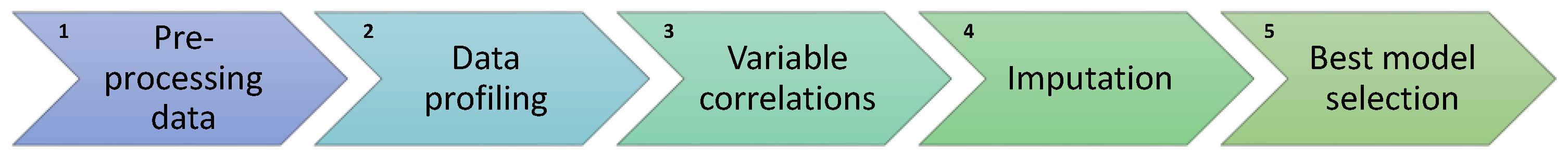
2.1. Methodology Description

The flowchart reported in Figure 1 describes the methodology adopted to accomplish the main goals of this study.

Five steps can be identified:

• Pre-processing data: The dataset was pre-processed before any analysis to deal with the different units, orders of magnitude, not unified variable names and different sampling frequencies.
• Data profiling: The dataset was analyzed with the aim of studying the distribution of the variables, their missing data and data quality (the dataset is described in Section 2.2, and the results of this step are reported in Section 3.1).
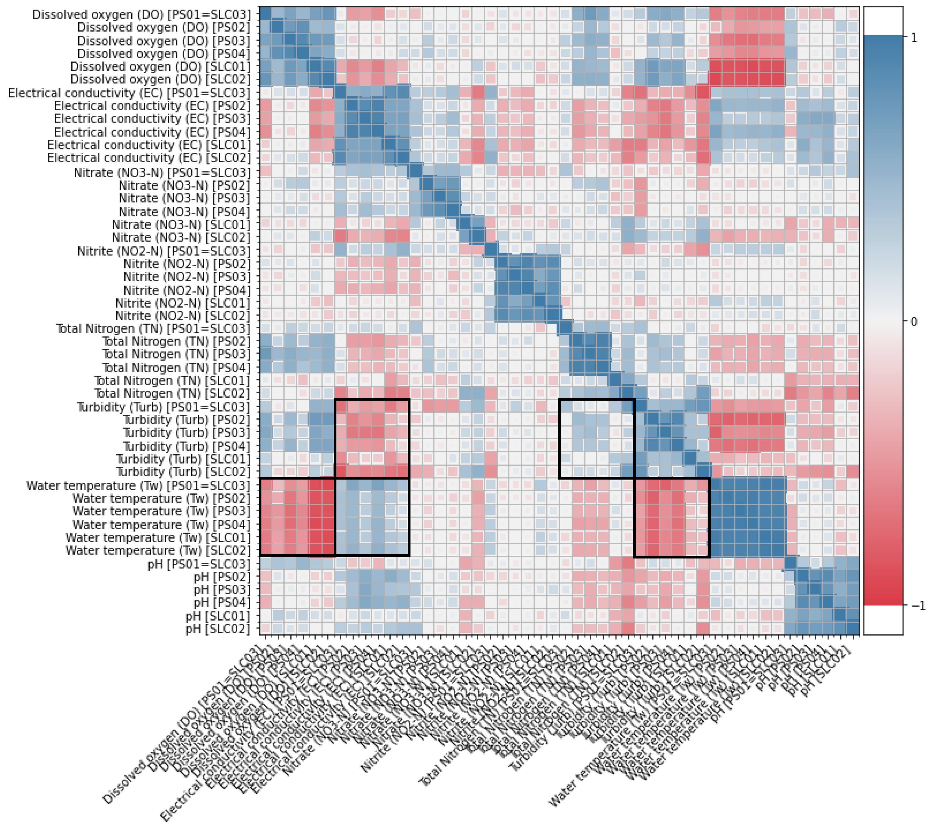
• Variable correlations: Correlations among variables were considered to help the multivariate imputation techniques (Section 2.5).
• Imputation: The selected imputation models were assessed, and their loss functions were computed (the imputation techniques and the imputation performance evaluation are described in Section 2.3 and Section 2.4, respectively).
• Best model selection: For each variable at each monitoring site, the model with the highest performance was selected as “the best model” (Section 3.2).

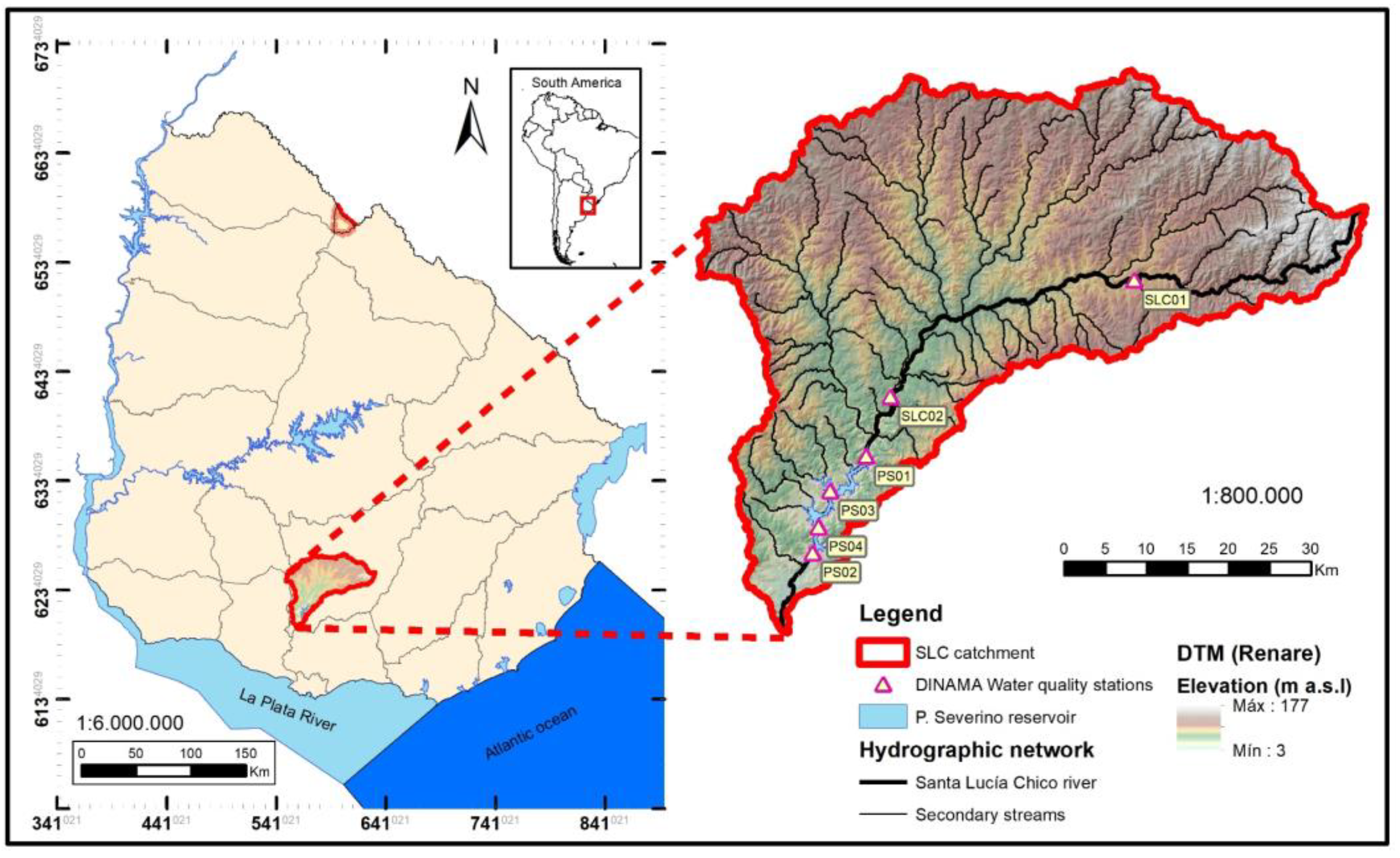
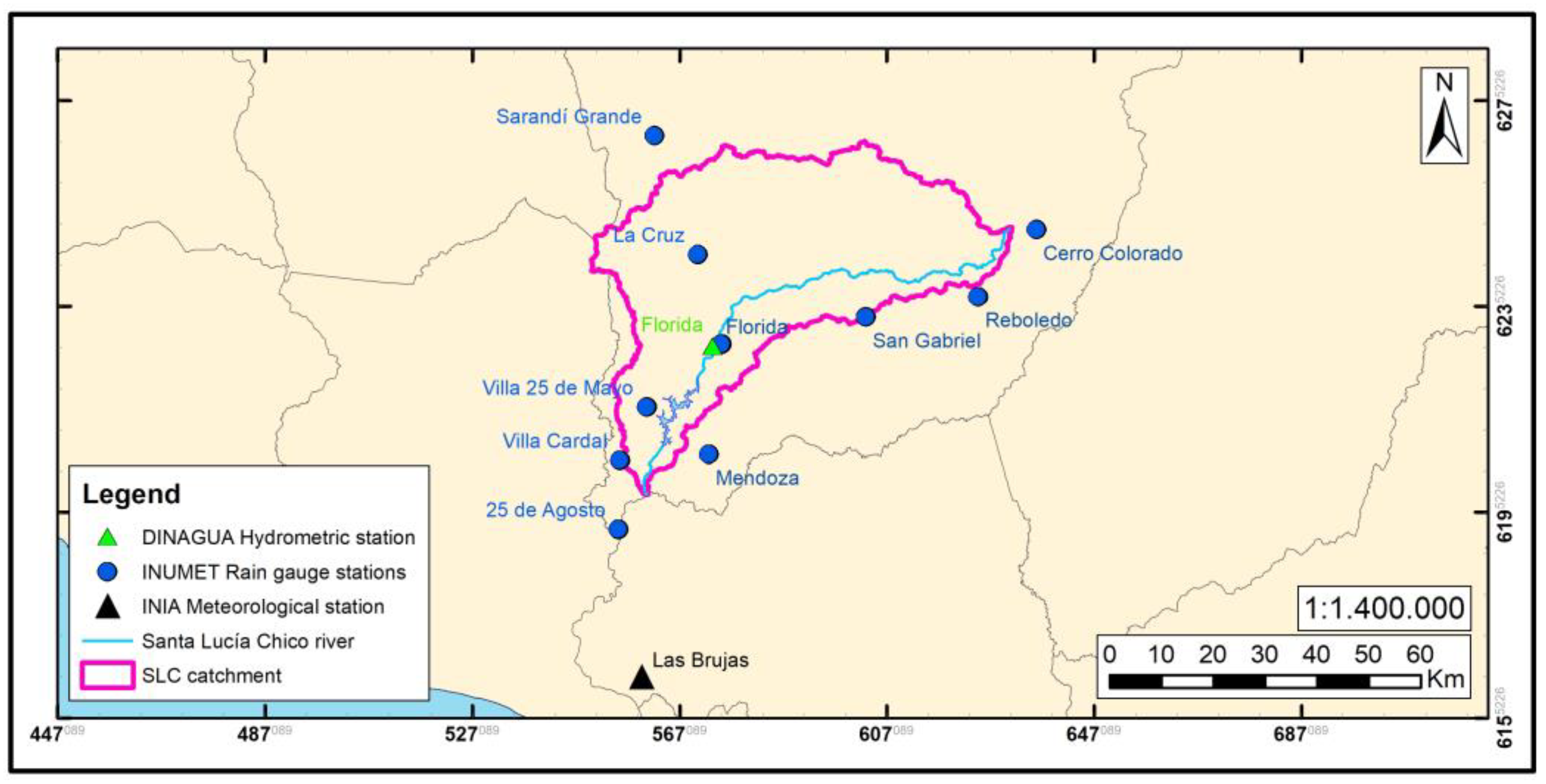
2.2. Dataset Description

Uruguay has a humid subtropical climate (Cfa, according to the Köppen climate classification) with a mean temperature in the warmest month equal to 22 °C or higher [18]. The study area is characterized by total annual precipitation that varies between 1000 mm and 1500 mm and a temperature that can vary between 3 °C and 30 °C [19]. The region has a landscape of smooth hills with an average slope equal to 2.68%.

The water-quality dataset used in this study includes the following physical and chemical variables: water temperature (T_w) [°C], electrical conductivity (EC) [µS/cm], pH, dissolved oxygen (DO) [mg/L], total nitrogen (TN) [mg/L], nitrite (NO₂⁻) [mg/L], nitrate (NO₃⁻) [mg/L] and turbidity (Turb) [NTU]. It was recorded by the Uruguayan National Environment Board (DINAMA) and is freely downloadable from the National Environmental Observatory (OAN) [20]. Data were collected from 2014 to 2020, with a bi-monthly frequency, at six monitoring stations located along the Santa Lucía Chico river, Uruguay. This is a mixed lotic and lentic system with wide national importance since its waters flow into the Paso Severino reservoir, the primary national drinking water source [19,21,22,23]. The first three upstream monitoring stations (SLC01, SLC02 and PS01) are located before the reservoir; the other three stations (PS03, PS04 and PS02) are located in the lake (Figure 2).

The percentage of missing values detected for each variable at all monitoring stations is reported in

Table 1. Percentage of missing data for the variables under study at the six monitoring stations (period 2014–2020).

Variable		% Missing Data
		SLC01	SLC02	PS01	PS03	PS04	PS02
Physical	Tw	51.5	51.5	64.7	57.6	57.6	59.1
	EC	51.5	51.5	64.7	57.6	57.6	57.6
	pH	52.9	52.9	66.2	59.1	59.1	59.1
	DO	51.5	51.5	64.7	57.6	57.6	57.6
	Turb	52.9	52.9	66.2	60.6	60.6	59.1
Chemical	TN	52.9	52.9	66.2	60.6	60.6	59.1
	NO2−	51.5	51.5	64.7	59.1	59.1	57.6
	NO3−	51.5	51.5	64.7	59.1	59.1	57.6

.

Some hydro-meteorological variables that may influence the water-quality variables under study were also considered to support the multivariate techniques. In particular, air temperature (T_a) (minimum, average, maximum) [°C], solar radiation (SR) [cal/cm²/d] and heliophany (Hel) (sunshine hours) [h] were used for T_w imputation. These data were collected daily by the National Institution of Agricultural Research (INIA) and have no missing values. T_a along with daily evapotranspiration (ET) data, also calculated from INIA (time series characterized by 0.1% of missing data), were considered for the imputation of Turb. Streamflow (Q) [m³/s] was considered for the imputation of TN, NO₂⁻, NO₃⁻ and Turb. This time series was measured three times a day by the Uruguay National Water Board (DINAGUA) and is characterized by a neglectable percentage of missing data (5.6%).

Furthermore, precipitation records (P) from the Uruguayan Institute of Meteorology (INUMET) were considered for Turb imputation. The time series observed at the ten selected monitoring stations have a percentage of missing data that varies between 0.0% and 8.6% in the considered time window (2014–2020). The location of the INIA, DINAGUA and INUMET monitoring stations is represented in Figure 3.

2.3. Imputation Techniques

Since the best model for imputing any kind of variable does not exist [24], we evaluated several statistical and machine-learning algorithms (single and multiple imputation) to accomplish the objective of this study. The selected models are Inverse distance weighting (IDW), Random Forest regressor (RFR), Ridge regressor (RR), Bayesian ridge (BR), AdaBoost (AB), Huber regressor (HR), Support vector regressor (SVR), TheilSen regressor (TSR) and k-nearest neighbors regressor (KNNR). All of them have proved to be suitable for non-linear environmental variables, and some of them for cases characterized by a high percentage of missing data. Furthermore, they are already programmed and freely available in Phyton. Unless a software library is explicitly mentioned, scikit-learn was adopted to implement the algorithms [25]. We now briefly describe each of the imputation methods.

Inverse Distance Weighting (IDW): It is a deterministic univariate interpolation method. Missing samples at the target station (s) are computed from the observed values at neighboring stations. The weighting is assigned to the data using a weighting power that controls how the weighting factors decrease as the distance from station s increases [26]. This model was run in R, by using gstat library (function: gstat.idw).

Random Forest Regressor (RFR): It is a supervised learning algorithm that uses an ensemble learning method for regression. Such a method is a technique that combines predictions from multiple Decision Tree algorithms to improve the overall prediction and control overfitting. The decision trees run in parallel with no interaction among them and the mean of all the predictions is returned [27] (function: sklearn.ensemble.RandomForestRegressor).

Ridge Regressor (RR): It is a technique for analyzing multiple regressions of highly correlated data. It trains a regression model that aims to minimize the least-squares function with an additional regularization term given by the sum of the values’ squares (L2 norm) [28] (function: sklearn.linear_model.Ridge).

Bayesian Ridge (BR): It is an estimator that assumes and predicts the target by calculating its probability distribution during training. This method can cope with data sparsity more effectively than other methods. [29] (function: sklearn.linear_model.BayesianRidge).

AdaBoost (AB): It is an estimator that starts fitting a decision tree regressor on the original dataset and then fits additional copies of the regressor on the same slightly modified dataset. Depending on the correctness of the last prediction, samples that are difficult to predict become more relevant as the training continues. The mean of all the models’ predictions is returned [30] (function: sklearn.ensemble.AdaBoostRegressor).

Huber Regressor (HR): It is an algorithm that trains a linear model which optimizes the mean squared error (L2 error) for samples whose error is lower than a given threshold (d) and the mean absolute error (L1 error) for samples whose error is greater than d. In this way, the optimized function is not heavily influenced by outliers while not completely ignoring their effect [31] (function: sklearn.linear_model.HuberRegressor).

Support Vector Regressor (SVR): It is an estimator that focuses on minimizing the coefficients. More specifically, it considers the l2-norm of the coefficient vector, not the squared error. The error term is handled instead in the constraints, where the absolute error is set to less than or equal to a specified margin (maximum error). The latter can be adjusted to obtain the desired accuracy of the model. [32] (function: sklearn.svm.SVR).

TheilSen Regressor (TSR): It is a regressor that makes its estimation by calculating the slopes and intercepts of a subpopulation of all possible combinations of some subsample points. The final slope and intercept are then defined as the spatial median of these slopes and intercepts. It is robust against outliers compared to other linear regressors [33] (function: sklearn.linear_model.TheilSenRegressor).

K-Nearest Neighbors Regressor (KNNR): It is a regressor that calculates the distance (using all variables) from the target point to the others and makes a prediction by interpolating the nearest neighbors in the dataset [34] (function: sklearn.neighbors.KNeighborsRegressor).

2.4. Imputation Performance Evaluation

To compare the accuracy of the implemented techniques in reconstructing missing water-quality data, Kling-Gupta efficiency (KGE), percent bias (PBIAS) and the Nash-Sutcliffe efficiency (NSE) were used. The latter was employed as the objective function since it is the most restrictive [35], while KGE and PBIAS were both used for validation. Equations (1)–(3) present these metrics, where x_i^o is the ith observed value, x_i^c is the ith computed (or imputed) value, $\overline{x^o}$ is the mean of observed values and n is the testing-dataset size. Being (μ^c,σ^c) and (μ^o,σ^o) the first two statistical moments (mean and standard deviation) of x^c and x^o, respectively, r is the linear correlation between observations and imputations, α is a measure of the flow variability error (α = σ^c/σ^o), β is a bias term (β = μ^c/μ^o).

$$NSE=1-\frac{{{\displaystyle \sum }}_{i=1}^n{\left(x_i^o-x_i^c\right)}^2}{{{\displaystyle \sum }}_{i=1}^n{\left(x_i^o-\overline{x^o}\right)}^2}$$

(1)

$$KGE=1-\sqrt{{\left(r-1\right)}^2+{\left(\alpha -1\right)}^2+{\left(\beta -1\right)}^2}$$

(2)

$$PBIAS=100\times \frac{{{\displaystyle \sum }}_{i=1}^n\left(x_i^o-x_i^c\right)}{{{\displaystyle \sum }}_{i=1}^n\left(x_i^o\right)}$$

(3)

NSE varies between −∞ and 1. If NSE is 1, the imputed values match the records perfectly. If NSE is 0, the imputed values are as good as the observation mean. If NSE is negative, the observation mean is a better predictor than imputed values. Therefore, higher NSE values are desirable since they indicate a more accurate imputation model [36,37].

Unlike NSE, there are not well-defined KGE thresholds that define a “good” model. For this reason, the current literature tends to interpret KGE values similarly to NSE: negative values indicate “bad” model performance, while positive values indicate “good” model performance [38,39,40]. However, a recent study by Knoben et al. [41] found that all model results with −0.41 < KGE < 1 could be considered good performance.

The optimal value of PBIAS is 0, with lower values indicating accurate model imputation. Positive values denote an underestimation bias of the model, and negative values indicate an overestimation bias of the model [42].

Table 2. Evaluation metrics and associated performance ratings.

Performance Rating	Physical Water Quality Variables	Chemical Water Quality Variables
NSE
Very good	NSE > 0.80	NSE > 0.65
Good	0.70 < NSE ≤ 0.80	0.50 < NSE ≤ 0.65
Satisfactory	0.45 < NSE ≤ 0.70	0.35 < NSE ≤ 0.50
Unsatisfactory	NSE ≤ 0.45	NSE ≤ 0.35
PBIAS
Very good	|PBIAS| < 10	|PBIAS| < 15
Good	10 ≤ |PBIAS| < 15	15 ≤ |PBIAS| < 20
Satisfactory	15 ≤ |PBIAS| < 20	20 ≤ |PBIAS| < 30
Unsatisfactory	|PBIAS| ≥ 20	|PBIAS| ≥ 30
KGE
Satisfactory/Good	KGE ≥ −0.41	KGE ≥ −0.41
Unsatisfactory	KGE < −0.41	KGE < −0.41

summarizes the performance evaluation criteria for NSE, KGE and PBIAS, used in this work, defined according to the standard review [36,41,42].

2.5. Helper Variables for the Imputation Process

Considering the correlations among water-quality variables, multivariate techniques exploited them for completing the missing values with the other existing water-quality observations. Spearman correlation was employed to evaluate possible correlations among water-quality variables, as it is a non-linear technique able to avoid overshadowing critical variable relationships. The aid variables considered in this study are framed in black in Figure 4. In particular, T_w and Turb influence EC in surface waters. An increase in T_w causes an increase in the mobility of the ions present in the water. An increase in T_w may also produce an increment in the number of ions due to molecule dissociation. As the EC depends on these factors, an increase in T_w leads to an increase in EC [43,44]. Furthermore, EC represents the ability of a liquid to conduct an electric charge; this ability depends on dissolved ion concentration, which is usually measured as total dissolved solids (TDS) [45]. Considering that TDS are highly correlated with Turb, we can assume that EC is also affected by Turb.

Furthermore, DO was considered dependent on T_w: the higher T_w, the lower DO. This is justified by the fact that cold water can hold more DO than warm water. In the cold season, when T_w is low, the DO concentration is high. In the warm season, when T_w is high, the DO concentration is often lower [19].

The variables Turb and T_w are also highly correlated. In general, Turb is known as a proxy of the amount of suspended solids in water. Such suspended particles in water bodies absorb heat from solar radiation more efficiently than water. The heat is then transferred from the particles to water molecules, increasing the surrounding water temperature [46].

Other correlations considered were the ones between TN-Turb, TN–NO₂⁻ and TN-NO₃⁻ (even though the last two were not highlighted in the correlation matrix). This is justified by the fact that TN represents the sum of dissolved and particle-bound nitrogen.

Moreover, as we have already mentioned in Section 2.1, we also considered hydro-meteorological variables aid for the imputation process since they may influence the water-quality variables under study. Particularly, Tw is deemed to be mainly affected by Ta, Hel and SR. Turb, TN, NO₂⁻ and NO₃⁻ are influenced by Q. Considering that NO₂⁻ and NO₃⁻ are part of the dissolved inorganic nitrogen (DIN), their correlation with streamflow is clear: the higher the Q, the lower the ions concentration, due to the dilution process [19]. Being TN the sum of dissolved and particle-bound nitrogen, we aided the imputation process of the latter by including Turb data. It is often assumed that these constituents positively affect river discharge, considering the importance of overland runoff in transporting sediments [47]. For this reason, we are considering Q as a supporting variable for Turb imputation.

In their study carried out in Santa Lucía Chico watershed, Gorgoglione et al. [19] found a seasonality of Turb values with higher values during the cold season. This was justified by the fact that in this season, frequent extreme precipitation events occur and, along with higher soil humidity due to low temperature, this causes a higher runoff and, therefore, a more significant amount of detached and washed-off sediments. For this reason, Turb imputation is also aided by ET, P and T_a data (apart from Q as previously explained).

A summary of the supporting variables taken into account for the imputation process is represented in

Table 3. Helper variables considered in the imputation process.

Variable to Impute	Helper Variable
Water temperature (Tw)	Air temperature (Ta)
	Solar radiation (SR)
	Heliophany (Hel)
	Turbidity (Turb)
Electrical Conductivity (EC)	Water temperature (Tw)
	Turbidity (Turb)
Dissolved oxygen (DO)	Water temperature (Tw)
Nitrite (NO2−)	Streamflow (Q)
Nitrate (NO3−)	Streamflow (Q)
Turbidity (Turb)	Streamflow (Q)
	Precipitation (P)
	Air temperature (Ta)
	Evapotranspiration (ET)
Total Nitrogen (TN)	Nitrite (NO2−)
	Nitrate (NO3−)
	Turbidity (Turb)
	Streamflow (Q)

.

3. Results and Discussion

3.1. Dataset Profiling

The dataset considered for this study is formed by 48 time series (8 water-quality variables × 6 monitoring stations). Therefore, from now on, we will call “variable,” “feature,” or “attribute,” a particular time series that refers to a water-quality variable recorded at one monitoring station (e.g., T_w observed at SLC01 monitoring station will be T_w[SLC01]). The data profiling process was programmed and run in Python 3.8, using the pandas_profiling library [48].

With the aim of showing the high temporal and spatial variability of the water-quality variables under study, we reported the box-plot representation at the six monitoring stations through the analyzed period (2014–2020) (Figure 5). From all the pollutant plots presented, it is interesting to identify two different groups of behavior: the three monitoring sites situated in the reservoir show different patterns compared to those that characterize the stations located upstream of the reservoir. Furthermore, T_w and DO are the only pollutants showing a strong intra- and inter-annual seasonality, while we cannot identify a clear pattern for the other contaminants under study. It is essential to highlight the high nutrient contribution of PS01 (TN, NO₂⁻, NO₃⁻), where the biggest city of the watershed is located (Florida, that with a population of over 33,000, is home to almost half of the inhabitants of the region). It is known that urbanized areas are sources of nitrogen due to atmospheric deposition, lawn fertilizer application, wastewater effluent and leaky sewage infrastructure [49]. Turb shows a minor temporal pattern through the years, with the highest values registered in the monitoring stations located upstream of the reservoir (SLC01, SLC02 and PS01).

To better understand and justify the high spatio-temporal variability of the attributes under study, we analyzed the seasonality of the hydro-meteorological parameters used as helper variables in the imputation process (ET, Hel, T_a, SR, P and Q) (Figure 6). As mentioned in Section 2.1., precipitation-time series observed at ten monitoring stations were adopted for this study. For the sake of clarity, in Figure 6, we are only presenting the P boxplots related to Florida station since it is the barycentric one of the watershed.

In these plots, the “winter” period includes the fall and winter seasons (April–May–June–July–August–September), and the “summer” time window considers the spring and summer seasons (October–November–December–January–February–March). As expected, the meteorological variables ET, Hel, T_a and SR show a strong seasonal pattern, with lower values in winter and higher values in summer. This behavior is not explicit for P and Q. They do not present an evident seasonality, but it is possible to state that in winter, extreme rainfall events and, therefore, major runoff events occur more frequently than in summer. This is justified by the fact that in the cold season, the higher soil humidity due to low temperature causes a higher runoff.

The strong seasonality of ET, Hel, T_a and SR justifies the strong intra- and inter-annual seasonality of T_w and DO since the former parameters are used as helper variables of the latter ones. The minor temporal pattern showed by Turb is explained by the fact that it depends on ET and T_a, characterized by a strong seasonality, and Q and P, which only present extreme events in winter, without showing a solid temporal pattern.

3.2. Imputation Results

To evaluate the performance of the different imputation models adopted and to choose the best one for each feature, k-fold cross-validation with k = 10 was used in this study. If a time series was characterized by less than 100 records, we adopted a repeated k-fold cross-validation, always with k = 10. This method repeats the k-fold cross-validation process multiple times and reports the mean performance across all folds and all repeats [50]. The dataset was min-max normalized before any analysis to deal with the different units and orders of magnitude. The winning (best) models were the ones with the optimal hyper-parameters, i.e., those with the highest NSE (objective function). As a result, the best model with the highest accuracy was selected for each feature and validated by calculating KGE and PBIAS. The outcomes of this methodology are represented by augmented time series for all the water-quality variables, characterized by one-month frequency (i.e., the frequency was doubled up). The methodology adopted in this study was implemented using Python programming language on a desktop computer (Ubuntu Operating System, 16 GB of RAM and Intel i3 Processor).

In

Table 4. Best imputation models and corresponding goodness-of-fit indicator values per variable.

Variable	Station	Model	NSE	NSE Rating	PBIAS	PBIAS Rating	KGE	KGE Rating
Tw	SLC01	Random Forest Regressor	0.95	Very good	0.09	Very good	0.91	Good
	SLC02	IDW	0.97	Very good	−2.54	Very good	0.95	Good
	PS01	IDW	0.95	Very good	−3.77	Very good	0.94	Good
	PS03	IDW	0.98	Very good	−0.21	Very good	0.96	Good
	PS04	IDW	0.98	Very good	1.49	Very good	0.96	Good
	PS02	IDW	0.97	Very good	0.89	Very good	0.93	Good
EC	SLC01	SVR	0.67	Satisfactory	−0.12	Very good	0.76	Good
	SLC02	SVR	0.71	Good	0.43	Very good	0.67	Good
	PS01	Ridge	0.67	Satisfactory	−1.70	Very good	0.77	Good
	PS03	Ridge	0.85	Very good	1.35	Very good	0.86	Good
	PS04	IDW	0.94	Very good	4.71	Very good	0.87	Good
	PS02	IDW	0.89	Very good	−3.89	Very good	0.88	Good
pH	SLC01	Bayesian Ridge	0.39	Unsatisfactory	−0.63	Very good	0.54	Good
	SLC02	Random Forest Regressor	0.75	Good	0.95	Very good	0.80	Good
	PS01	Random Forest Regressor	0.25	Unsatisfactory	0.44	Very good	0.40	Good
	PS03	Bayesian Ridge	0.66	Satisfactory	−0.31	Very good	0.78	Good
	PS04	IDW	0.68	Satisfactory	−1.10	Very good	0.79	Good
	PS02	Huber Regressor	0.65	Satisfactory	−3.29	Very good	0.77	Good
DO	SLC01	Bayesian Ridge	0.81	Very good	−2.79	Very good	0.83	Good
	SLC02	Random Forest Regressor	0.73	Good	−1.80	Very good	0.73	Good
	PS01	AdaBoost	0.27	Unsatisfactory	−1.65	Very good	0.48	Good
	PS03	Ridge	0.80	Good	−0.15	Very good	0.86	Good
	PS04	Huber Regressor	0.89	Very good	−0.28	Very good	0.89	Good
	PS02	IDW	0.69	Satisfactory	−0.24	Very good	0.79	Good
TN	SLC01	IDW	0.19	Unsatisfactory	2.72	Very good	0.49	Good
	SLC02	Ridge	0.65	Good	1.90	Very good	0.72	Good
	PS01	Random Forest Regressor	−0.35	Unsatisfactory	−0.91	Very good	−0.10	Good
	PS03	IDW	0.63	Good	−7.79	Very good	0.75	Good
	PS04	Random Forest Regressor	0.77	Very good	−1.38	Very good	0.71	Good
	PS02	IDW	0.70	Very good	−15.22	Good	0.71	Good
NO2−	SLC01	Huber Regressor	0.59	Good	−0.83	Very good	0.62	Good
	SLC02	Random Forest Regressor	0.36	Satisfactory	−10.79	Very good	0.54	Good
	PS01	KNN	−0.31	Unsatisfactory	25.94	Satisfactory	0.02	Good
	PS03	TheilSen Regressor	0.74	Very good	1.09	Very good	0.72	Good
	PS04	KNN	0.92	Very good	3.35	Very good	0.86	Good
	PS02	Huber Regressor	0.75	Very good	−4.53	Very good	0.78	Good
NO3−	SLC01	TheilSen Regressor	0.21	Unsatisfactory	13.68	Very good	0.33	Good
	SLC02	Huber Regressor	0.42	Satisfactory	−4.95	Very good	0.58	Good
	PS01	Random Forest Regressor	0.10	Unsatisfactory	5.14	Very good	0.36	Good
	PS03	IDW	0.69	Very good	−0.80	Very good	0.80	Good
	PS04	Huber Regressor	0.80	Very good	−1.08	Very good	0.84	Good
	PS02	SVR	0.61	Good	−1.57	Very good	0.75	Good
Turb	SLC01	SVR	−0.10	Unsatisfactory	−1.93	Very good	0.03	Good
	SLC02	SVR	0.56	Satisfactory	−5.74	Very good	0.67	Good
	PS01	IDW	−0.18	Unsatisfactory	−45.97	Unsatisfactory	0.35	Good
	PS03	IDW	0.66	Satisfactory	−12.30	Good	0.71	Good
	PS04	IDW	0.85	Very good	3.94	Very good	0.88	Good
	PS02	IDW	0.88	Very good	−3.27	Very good	0.87	Good

, we report, for each variable, the winning model with the corresponding values of the goodness-of-fit indicators calculated and the corresponding rating based on Table 3.

Considering the NSE rating, the imputation performance is overall adequate. Tw at the six monitoring stations was the best-imputed variable, showing “very good” performance. The strong daily and annual seasonality that characterizes this variable makes its simulation and, therefore, its imputation less difficult. The correlation that exists between Tw and EC (an increase in Tw leads to an increase in EC) [43,44] is reflected in the “good” performance of this variable at the six monitoring sites (“satisfactory” at SLC01 and PS01; “good” at SLC02; “very good” at PS03, PS04 and PS02). The imputation process for the other water-quality variables shows different results. It is noteworthy that the performance is always notable at the three monitoring stations located in the reservoir of Paso Severino (PS03, PS04 and PS02); while the imputation can sometimes be “unsatisfactory” at the stations located upstream, along Santa Lucía Chico river (SLC01, SLC02 and PS01). This outcome can be attributed to the different hydrologic-response times considering the location of the measurement sites. The time base of the hydrographs observed at Florida hydrometric station (Figure 3) is overall equal to 6 days and it generally does not vary with the change of the flow magnitude. Ríos [51] found that, on average, the renewal time of the Paso Severino reservoir ranges between 2 to 8 weeks. He also observed that during storm events, the renewal time could be a few days long, while it can last several months during dry periods. SLC01 and SLC02 are located several kilometers upstream of the reservoir, where the water body has a fluvial behavior associated with a lotic ecosystem. While PS02, PS03 and PS04 are located within the reservoir, where the water body is lacustrine, associated with a lentic ecosystem. The validation of the imputation process was outstanding, showing overall “very good” results in terms of the PBIAS and KGE ratings.

A box-plot representation of the model performance (NSE, PBIAS and KGE) is represented in Figure 7. More than 76% of the imputed data is characterized by NSE > 0.45 (it is at least “satisfactory”), and more than 92% of the imputed data has a positive NSE, meaning that for almost all the imputations, our methodology is better than the mean function used as an imputer. The validation results were notable. Considering PBIAS ratings, more than 96% of the imputed data can be considered at least “satisfactory” and more than 88% “very good.” In terms of KGE ratings, all the imputations are considered “good.”

IDW outperformed the other models in most cases (17 times), followed by RFR (8 times), HR (6 times), SVR (5 times) and RR (4 times). A possible explanation is that IDW is the only model that, in addition to considering temporal information, includes spatial information by looking at neighboring stations to support the imputation process. The other implemented machine-learning models won almost the same number of times (same order of magnitude).

3.3. Further Discussion

Effective water-resource management requires the analysis of a large number of water-quality information over space and time. However, in many parts of the world, particularly in developing countries, the monitoring of water-quality variables is usually characterized by few monitoring stations over the territory, where observations are recorded with a low frequency and are characterized by an important percentage of missing data. Therefore, in this study, we evaluated the performance of several statistical and machine-learning techniques (univariate and multivariate) in imputing a water-quality dataset characterized by eight water quality variables measured at six monitoring stations. Particularly, we aimed to augment the water-quality dataset, from bi-monthly to monthly frequency. The percentage of missing values ranges between 50% and 70% (high missingness percentage), and the water-quality variables are characterized by a high temporal and spatial distribution. The study area considered was one of the most critical Uruguayan watersheds, Santa Lucía Chico, since it provides water to more than 60% of the national population. This was an interesting study area to analyze since it is a mixed lotic and lentic system and the six monitoring stations are located along the mainstream (SLC01, SLC02 and PS01) and in the reservoir (PS03, PS04 and PS02). In this way, it was appealing to assess the performance of several models in these two different surface-water bodies.

There are few related works on the imputation of water-quality data, and they are relatively recent. In 2012, Srebotnjak et al. [17] showed that hot-deck imputation can improve geographical coverage of a country-level water quality index, calculated considering dissolved oxygen, electrical conductivity, pH, total phosphorus and total nitrogen. This water-quality index is a composite indicator to track water quality over time and space, easily interpretable since it varies from 0 to 100. Still, it does not allow a detailed analysis of each water-quality variable used to calculate it. Therefore, this type of index does not allow us to answer scientific questions such as which compounds are significant indicators for specific land use categories or the spatio-temporal behavior of a particular problematic compound in a particular area of study. To overcome these limitations, we decided to directly impute each water-quality variable and not a global index, which allows us to use the imputed data for more advanced analyses.

In 2015, Tabari and Talaee [16] obtained acceptable results (RMSE ranges between 0.016 and 4475) in imputing a large dataset of water-quality information (13 variables) measured, with a monthly frequency, at five monitoring sites along the Maroon River (Southwest of Iran). It should be noted that this study has already adopted the concept of helper variables to improve the imputation process based on the correlations among water-quality variables. The correlation between EC and Turb that we used in our analysis is confirmed in this study. In Tabari and Talaee [16], the results were insufficient for EC, Turb and total dissolved solids (TDS) at all monitoring stations, showing RMSE values between 100 and higher than 4000. They employed only two artificial neural networks as imputation models: multilayer perceptron and radial bias function. In our study, we improved such results using more imputation techniques and founding that SVR model shows better performance for EC and Turb.

In 2019, Ratolojanahary et al. [7] tackled for the very first time the problem of high rate missingness (higher than 80%) in a water-quality dataset of a drinking water well employing four machine learning models (RF, KNNR, SVR and boosted regression trees, similar to our AB). Their outcomes showed that SVR provides the best performance (notably in terms of average prediction error). However, this study does not introduce the temporal dimension into the imputation process, and, therefore, temporal variability of water-quality parameters is not considered a challenge. Spatial variability is also not addressed, as the authors analyzed water well. These aspects are included in our study. Furthermore, we confirm that the performance of SVR is better than AB and KNNR in the imputation of water quality data.

It is also important to note that our work pioneered the use of IDW for water-quality data imputation, and this method performed the best among all the methods analyzed. Some recent works proposed using IDW to interpolate water quality in scenarios where spatial variability may be negligible, as in the case of lakes [52] or where temporal variability is low, as in the case of groundwater [53].

Some of the correlations found in our work were also reported in previous studies in the same study area [19,21,23,54]: a robust correlation among nitrogen compounds, in its dissolved and particle-bound form; a strong inverse correlation between by T_w and DO.

4. Conclusions

In this study, we tackled the challenge of data imputation in a multivariate water-quality dataset characterized by a high percentage of missing data (between 50% and 70%). In particular, the variables T_w, EC, pH, DO, TN, NO₂⁻, NO₃⁻ and Turb of six monitoring stations located along the Santa Lucía Chico river (Uruguay) were considered for this study. Adopting a multi-model approach was crucial since the best model for imputing any water-quality variable does not exist. The statistical and machine-learning models implemented were IDW, RFR, RR, BR, AB, HR, SVR and KNNR.

The imputation outcomes were overall adequate. More than 76% of the imputed data can be considered “satisfactory” (NSE > 0.45). This was validated by calculating PBIAS (>96% of the imputed data is “satisfactory”) and KGE (all the imputations are considered “good”). It is interesting to notice that the performance is always remarkable at the three monitoring stations located in the Paso Severino reservoir, while they may be “unsatisfactory” at some monitoring stations located along the Santa Lucía Chico river (upstream the reservoir). Among the implemented models, IDW was chosen as the best model 17 times since it is the only model that considers the temporal and spatial variability that characterizes the variables under study.

This study paves the path to future water-quality research in the watershed under study (e.g., implementation of reliable modeling tools, water-quality prediction and scenario analysis). Hopefully, the results obtained in this work will help water managers and researchers worldwide make the most of existing water-quality data to improve modeling and generate effective pollution-control strategies.

Our current results are promising, but we believe that it is possible to improve the present methodology by integrating physical knowledge that considers the spatial information of the available water-quality data. Our future work intends to transform the current approach, based on machine learning, into a hybrid method where the data-driven techniques incorporate physical aspects during their training.

References

1. Whitehead, P.; Dolk, M.; Peters, R.; Leckie, H. Water Quality Modelling, Monitoring, and Management. In Water Science, Policy, and Management; Dadson, S.J., Garrick, D.E., Penning-Rowsell, E.C., Hall, J.W., Hope, R., Hughes, J., Eds.; John Wiley & Sons Ltd.: Hoboken, NJ, USA, 2019. [Google Scholar]
2. Gorgoglione, A.; Castro, A.; Chreties, C.; Etcheverry, L. Overcoming Data Scarcity in Earth Science. Data 2020, 5, 5. [Google Scholar] [CrossRef] [Green Version]
3. Teegavarapu, R.S.V.; Aly, A.; Pathak, C.S.; Ahlquist, J.; Fuelberg, H.; Hood, J. Infilling missing precipitation records using variants of spatial interpolation and data-driven methods: Use of optimal weighting parameters and nearest neighbour-based corrections. Int. J. Climatol. 2018, 38, 776–793. [Google Scholar] [CrossRef]
4. Mital, U.; Dwivedi, D.; Brown, J.B.; Faybishenko, B.; Painter, S.L.; Steefel, C.I. Sequential imputation of missing spatio-temporal precipitation data using random forests. Front. Water 2020, 2, 20. [Google Scholar] [CrossRef]
5. Aguilera, H.; Guardiola-Albert, C.; Serrano-Hidalgo, C. Estimating extremely large amounts of missing precipitation data. J. Hydroinformatics 2020, 22, 578–592. [Google Scholar] [CrossRef] [Green Version]
6. Buhi, E. Out of sight, not out of mind: Strategies for handling missing data. Am. J. Health Behav. 2008, 32, 83–92. [Google Scholar] [CrossRef]
7. Ratolojanahary, R.; Ngouna, R.H.; Medjaher, K.; Junca-Bourié, J.; Dauriac, F.; Sebilo, M. Model selection to improve multiple imputation for handling high rate missingness in a water quality dataset. Expert Syst. Appl. 2019, 131, 299–307. [Google Scholar] [CrossRef] [Green Version]
8. Lo Presti, R.; Barca, E.; Passarella, G. A methodology for treating missing data applied to daily rainfall data in the Candelaro River Basin (Italy). Environ. Monit. Assess. 2010, 160, 1–22. [Google Scholar] [CrossRef] [PubMed]
9. Chen, F.W.; Liu, C.W. Estimation of the spatial rainfall distribution using inverse distance weighting (IDW) in the middle of Taiwan. Paddy Water Environ. 2012, 10, 209–222. [Google Scholar] [CrossRef]
10. Barrios, A.; Trincado, G.; Garreaud, R. Alternative approaches for estimating missing climate data: Application to monthly precipitation records in South-Central Chile. For. Ecosyst. 2018, 5, 28. [Google Scholar] [CrossRef] [Green Version]
11. Gong, G.; Mattevada, S.; O’Bryant, S.E. Comparison of the accuracy of kriging and IDW interpolations in estimating groundwater arsenic concentrations in Texas. Environ. Res. 2014, 130, 59–69. [Google Scholar] [CrossRef] [PubMed]
12. Aissia, M.-A.B.; Chebana, F.; Ouarda, T. Multivariate missing data in hydrology–Review and applications. Adv. Water Resour. 2017, 110, 299–309. [Google Scholar] [CrossRef] [Green Version]
13. Chivers, B.D.; Wallbank, J.; Cole, S.C.; Sebek, O.; Stanley, S.; Fry, M.; Leontidis, G. Imputation of missing sub-hourly precipitation data in a large sensor network: A machine learning approach. J. Hydrol. 2020, 588, 125126. [Google Scholar] [CrossRef]
14. Sattari, M.-T.; Rezazadeh-Joudi, A.; Kusiak, A. Assessment of different methods for estimation of missing data in precipitation studies. Hydrol. Res. 2017, 48, 1032–1044. [Google Scholar] [CrossRef]
15. Oriani, F.; Borghi, A.; Straubhaar, J.; Mariethoz, G.; Renard, P. Missing data simulation inside flow rate time series using multiple-point statistics. Environ. Model. Softw. 2016, 86, 264–276. [Google Scholar] [CrossRef] [Green Version]
16. Tabari, H.; Talaee, P.H. Recontrsuction of river water quality missing data using artificial neural networks. Water Qual. Res. J. Can. 2015, 50, 4. [Google Scholar] [CrossRef]
17. Srebotnjak, T.; Carr, G.; de Sherbinin, A.; Rickwood, C. A global Water Quality Index and hot-deck imputation of missing data. Ecol. Indic. 2012, 17, 108–119. [Google Scholar] [CrossRef]
18. Hastings, F.; Fuentes, I.; Perez-Bidegain, M.; Navas, R.; Gorgoglione, A. Land-Cover Mapping of Agricultural Areas Using Machine Learning in Google Earth Engine. In Computational Science and Its Applications—ICCSA 2020. ICCSA 2020. Lecture Notes in Computer Science; Gervasi, O., Murgante, B., Misra, S., Garau, C., Blečić, I., Taniar, D., Apduhan, B.O., Rocha, A.M.A.C., Tarantino, E., Torre, C.M., et al., Eds.; Springer: Cham, Switzerland, 2020; Volume 12252. [Google Scholar]
19. Gorgoglione, A.; Gregorio, J.; Ríos, A.; Alonso, J.; Chreties, C.; Fossati, M. Influence of land use/land cover on surface-water quality of Santa Lucía river, Uruguay. Sustainability 2020, 12, 4692. [Google Scholar] [CrossRef]
20. OAN—Observatorio Ambiental Nacional. Available online: https://www.dinama.gub.uy/oan/geoportal/ (accessed on 11 January 2021).
21. Goyenola, G.; Meerhoff, M.; Teixeira-de Mello, F.; González-Bergonzoni, I.; Graeber, D.; Fosalba, C.; Vidal, N.; Mazzeo, N.; Ovesen, N.B.; Jeppesen, E.; et al. Phosphorus dynamics in lowland streams as a response to climatic, hydrological and agricultural land use gradients. Hydrol. Earth Syst. Sci. Discuss. 2015, 12, 3349–3390. [Google Scholar]
22. Aubriot, L.; Delbene, L.; Haakonson, S.; Somma, A.; Hirsch, F.; Bonilla, S. Evolución de la eutrofización en el Río Santa Lucía: Influencia de la intensificación productiva y perspectivas. Innotec 2017, 14, 7–17. [Google Scholar] [CrossRef]
23. Gorgoglione, A.; Alonso, J.; Chreties, C.; Fossati, M. Assessing temporal and spatial patterns of surface-water quality with a multivariate approach: A case study in Uruguay. In Proceedings of the IOP Conference Series: Earth and Environmental Science, Changchun, China, 21–23 August 2020; Volume 612, p. 012002. [Google Scholar]
24. Wolpert, D.; Macready, W. No free lunch theorems for optimization. IEEE Trans. Evol. Comput. 1997, 1, 67–82. [Google Scholar] [CrossRef] [Green Version]
25. Pedregosa, F.; Varoquaux, G.; Gramfort, A.; Michel, V.; Thirion, B.; Grisel, O.; Blondel, M.; Prettenhofer, P.; Weiss, R.; Dubourg, V.; et al. Scikit-learn: Machine learning in Python. J. Mach. Learn. Res. 2011, 12, 2825–2830. [Google Scholar]
26. Bartier, P.M.; Keller, C.P. Multivariate interpolation to incorporate thematic surface data using inverse distance weighting (IDW). Comput. Geosci. 1996, 22, 195–799. [Google Scholar] [CrossRef]
27. Tang, F.; Ishwaran, H. Random Forest Missing Data Algorithms. Stat. Anal Data Min. 2017, 10, 363–377. [Google Scholar] [CrossRef]
28. Farebrother, R.W. Further results on the mean square error of ridge regression. J. R. Stat. Soc. 1976, 38, 248–250. [Google Scholar] [CrossRef]
29. Tipping, M.E. Sparse Bayesian Learning and the Relevance Vector Machine. J. Mach. Learn. Res. 2001, 1, 211–244. [Google Scholar]
30. Drucker, H. Improving Regressors using Boosting Techniques. In Proceedings of the Fourteenth International Conference on Machine Learning (ICML’97), Nashville, TN, USA, 8–12 July 1997; Morgan Kaufmann Publishers Inc.: San Francisco, CA, USA, 1997; pp. 107–115. [Google Scholar]
31. Art, O. A robust hybrid of lasso and ridge regression. Contemp. Math. 2007, 443, 59–72. [Google Scholar] [CrossRef] [Green Version]
32. Smola, A.J.; Schölkopf, B. A tutorial on support vector regression. Stat. Comput. 2004, 14, 199–222. [Google Scholar] [CrossRef] [Green Version]
33. Dang, X.; Peng, H.; Wang, X.; Zhang, H. Theil-Sen Estimators in a Multiple Linear Regression Model. Mater. Sci. 2009. Available online: https://www.semanticscholar.org/paper/THE-THEIL-SEN-ESTIMATORS-IN-A-MULTIPLE-LINEAR-MODEL-Wang-Dang/63167c5dbb9bae6f0a269237a9b6a28fa7e1ac20 (accessed on 2 June 2021).
34. Mucherino, A.; Papajorgji, P.J.; Pardalos, P.M. k-Nearest Neighbor Classification. In Data Mining in Agriculture; Springer Optimization and Its Applications, 34; Springer: New York, NY, USA, 2009. [Google Scholar]
35. Narbondo, S.; Gorgoglione, A.; Crisci, M.; Chreties, C. Enhancing physical similarity approach to predict runoff in ungauged watersheds in sub-tropical regions. Water 2020, 12, 528. [Google Scholar] [CrossRef] [Green Version]
36. Chen, H.; Luo, Y.; Potter, C.; Moran, P.J.; Grieneisen, M.L.; Zhang, M. Modeling pesticide diuron loading from the San Joaquin watershed into the Sacramento-San Joaquin Delta using SWAT. Water Res. 2017, 121, 374–385. [Google Scholar] [CrossRef]
37. Gorgoglione, A.; Bombardelli, F.A.; Pitton, B.J.L.; Oki, L.R.; Haver, D.L.; Young, T.M. Role of Sediments in Insecticide Runoff from Urban Surfaces: Analysis and Modeling. Int. J. Environ. Res. Public Health 2018, 15, 1464. [Google Scholar] [CrossRef] [Green Version]
38. Rogelis, M.C.; Werner, M.; Obregón, N.; Wright, N. Hydrological model assessment for flood early warning in a tropical high mountain basin. Hydrol. Earth Syst. Sci. Discuss. 2016, 1–36. [Google Scholar] [CrossRef] [Green Version]
39. Andersson, J.C.M.; Arheimer, B.; Traoré, F.; Gustafsson, D.; Ali, A. Process refinements improve a hydrological model concept applied to the Niger River basin. Hydrol. Process. 2017, 31, 4540–4554. [Google Scholar] [CrossRef] [Green Version]
40. Knoben, W.J.M.; Woods, R.A.; Freer, J.E. A Quantitative Hydrological Climate Classification Evaluated with Independent Streamflow Data. Water Resour. Res. 2018, 54, 5088–5109. [Google Scholar] [CrossRef] [Green Version]
41. Knoben, W.J.M.; Freer, J.E.; Woods, R.A. Technical note: Inherent benchmark or not? Comparing Nash-Sutcliffe and Kling-Gupta efficiency scores. Hydrol. Earth Syst. Sci. 2019, 23, 4323–4331. [Google Scholar] [CrossRef] [Green Version]
42. Moriasi, D.N.; Arnold, J.G.; Van Liew, M.W.; Bingner, R.L.; Harmel, R.D.; Veith, T.L. Model evaluation guidelines for systematic quantification of accuracy in watershed simulations. Soil Water Div. Asabe 2007, 50, 885–900. [Google Scholar]
43. Hayashi, M. Temperature-Electrical Conductivity Relation of Water for Environmental Monitoring and Geophysical Data Inversion. Environ. Monit. Assess. 2004, 96, 119–128. [Google Scholar] [CrossRef] [PubMed]
44. Beretta-Blanco, A.; Carrasco-Letelier, L. Relevant factors in the eutrophication of the Uruguay River and the Río Negro. Sci. Total Environ. 2021, 761, 143299. [Google Scholar] [CrossRef]
45. Bakhtiar Jemily, N.H.; Ahmad Sa’ad, F.N.; Mat Amin, A.R.; Othman, M.F.; Mohd Yusoff, M.Z. Relationship between Electrical Conductivity and Total Dissolved Solids as Water Quality Parameter in Teluk Lipat by Using Regression Analysis. In Progress in Engineering Technology; Abu Bakar, M., Mohamad Sidik, M., Öchsner, A., Eds.; Advanced Structured Materials; Springer: Cham, Switzerland, 2019; Volume 119, pp. 169–173. [Google Scholar]
46. Paaijmans, K.P.; Takken, W.; Githeko, A.K.; Jacobs, A.F. The effect of water turbidity on the near-surface water temperature of larval habitats of the malaria mosquito Anopheles gambiae. Int. J. Biometeorol. 2008, 52, 747–753. [Google Scholar] [CrossRef] [PubMed] [Green Version]
47. Lintern, A.; Wbb, J.A.; Ryu, D.; Liu, S.; Bende-Michl, U.; Waters, D.; Leahy, P.; Wilson, P.; Western, A.W. Key factors influencing differences in stream water quality across space. WIREs Water 2018, 5, e1260. [Google Scholar] [CrossRef] [Green Version]
48. Pandas_Profiling Library. Available online: https://github.com/pandas-profiling/ (accessed on 29 December 2020).
49. Reisinger, A.J.; Groffman, P.M.; Rosi-Marshall, E.J. Nitrogen-cycling process rates across urban ecosystems. FEMS Microbiol. Ecol. 2016, 92, 198. [Google Scholar] [CrossRef] [PubMed]
50. Refaeilzadeh, P.; Tang, L.; Liu, H. Cross-Validation. In Encyclopedia of Database Systems; Liu, L., Özsu, M.T., Eds.; Springer: Boston, MA, USA, 2009. [Google Scholar]
51. Río, A. Implementación de un Modelo Hidrodinámico Tridimensional en el Embalse de Paso Severino. Aportes Para la Modelación de Calidad de Agua. Master’s Thesis, Graduate Program of Applied Fluid Mechanics, Universidad de la República, Montevideo, Uruguay, 2019. Available online: https://www.colibri.udelar.edu.uy/jspui/handle/20.500.12008/21553 (accessed on 29 April 2021).
52. Jácome, G.; Valarezo, C.; Yoo, C. Assessment of water quality monitoring for the optimal sensor placement in lake Yahuarcocha using pattern recognition techniques and geographical information systems. Environ. Monit. Assess. 2018, 190, 259. [Google Scholar] [CrossRef] [PubMed]
53. Kanga, I.S.; Naimi, M.; Chikhaoui, M. Groundwater quality assessment using water quality index and geographic information system based in Sebou River Basin in the North-West region of Morocco. Int. J. Energ. Water Res. 2020, 4, 347–355. [Google Scholar] [CrossRef]
54. Barreto, P.; Dogliotti, S.; Perdomo, C. Surface water quality of intensive farming areas within the Santa Lucia River basin of Uruguay. Air Soil Water Res. 2017, 10, 1178622117715446. [Google Scholar] [CrossRef] [Green Version]
Figure 1. Methodology adopted for the imputation process.
Sustainability 13 06318 g001
Figure 2. Santa Lucía Chico river (Uruguay) and location of the six water-quality monitoring stations.
Sustainability 13 06318 g002
Figure 3. Location of the meteorological (INIA), hydrometric (DINAGUA) and pluviometric (INUMET) monitoring stations in Santa Lucía Chico.
Sustainability 13 06318 g003
Figure 4. Spearman correlation among water-quality variables.
Sustainability 13 06318 g004
Figure 5. Temporal and spatial variation of the water-quality variables.
Sustainability 13 06318 g005aSustainability 13 06318 g005b
Figure 6. Seasonality of the hydro-meteorological helper variables.
Sustainability 13 06318 g006
Figure 7. Box plots of model imputation performance (NSE, ǀPBIASǀ and KGE).
Sustainability 13 06318 g007