The Sensitivity of Vegetation Phenology to Extreme Climate Indices in the Loess Plateau, China

Abstract

Climate changes, especially increased temperatures, and precipitation changes, have significant impacts on vegetation phenology. However, the response of vegetation phenology to the extreme climate in the Loess Plateau in Northwest China remains poorly quantified. The research described here analyzed the spatial change in vegetation phenology and the response of vegetation phenology to climate change in the Loess Plateau from 2001 to 2018, using data from seven extreme climate indices based on the ridge regression method. The results showed that extreme climate indexes, TNn (yearly minimum value of the daily minimum temperature), TXx (yearly maximum value of the daily maximum temperature), and RX5day (yearly maximum consecutive five-day precipitation) progressively increased from 2001 to 2018 in the Loess Plateau region, but decrease trend was found in DRT (diurnal temperature range). The start of the growing season (SOS) of vegetation gradually advanced with precipitation from northwest to southeast, and the rate was +0.38 d/a. The overall vegetation end of the growing season (EOS) was delayed, and the trend was −2.83 d/a. The sensitivity of the different vegetation phenology to different extreme weather indices showed obvious spatial differences, the sensitivity coefficient of SOS being mainly positive in the region, whereas the sensitivity coefficient of EOS was negative generally. More sensitivity was found in the EOS to extreme climate indexes than in the SOS. Forest, shrubland and grassland have similar responses to DRT and TNn; namely, both SOS and EOS are advanced with the increase in DRT and delayed with the increase in TNn (the sensitivity coefficient is quite different) but have different responses to RX5day and TXx. These results reveal that extreme climate events have a greater impact on vegetation EOS than on vegetation SOS, with these effects varying with vegetation types. This research can provide a scientific basis for formulating a scientific basis for regional vegetation restoration strategies and disaster prediction on the Loess Plateau.

1. Introduction

The IPCC (Intergovernmental Panel on Climate Change) Fifth Assessment Report states that most parts of the world are experiencing climate change, especially sustained warming (the global average surface temperature increased by 0.72 °C from 1951 to 2012) [1,2]. Climate change includes meaning climate change and extreme climate change [3,4]. Some studies have shown that the impacts of extreme weather events are more obvious and direct than climate averages with increased frequency and intensity of extreme climate events [2,5]. Based on global climate change, more and more scholars devote themselves to research the dynamics of vegetation and its response to climate change [5].

As an opportunity to study seasonal changes in vegetation, status vegetation phenology not only determines the length of vegetation canopy photosynthesis but also plays an important role in the carbon balance of terrestrial ecosystems [6,7,8]. Climate change is one of the main drivers of vegetation growth, the effect of extreme climate changes vegetation dynamics appears to be more pronounced than climate change mean state [9,10]. The occurrence of extreme events can disrupt vegetation activity, advancing the flowering period of some species or even causing some species to fail to complete their flowering cycle [11]. Some researchers studying the Tibetan Plateau found that the end of the growing season (EOS) of vegetation is more influenced by extreme temperature events than extreme rainfall. An increase in the heat index of extreme temperature events leads to a delay in vegetation EOS, whereas an increased cold index can lead to an early end to vegetation EOS [12], with warmer days and nights similarly causing delayed fall phenology in Inner Mongolia [13]. A study of vegetation phenology in the United States found that an increase in daily maximum temperature had its main influence on an earlier vegetation start of the growing season (SOS) [14]. By studying the effects of drought, frost, heat, and humidity on fall phenology in Greenland, Xie et al. found that an increased cold index caused forests to end the growing season early, while increased heat index and drought stress delayed the dormancy of vegetation [15]. This shows that extreme climate events have a greater impact than averaged climate values on vegetation phenology in climate-change-sensitive areas. Therefore, the occurrence of extreme events may alter vegetation dynamics and carbon balance, which may lead to a shift from carbon sinks to carbon sources, such as the European heatwave event in 2003, Hurricane Katrina in 2005, and the 2019 Australian bushfires [16,17].

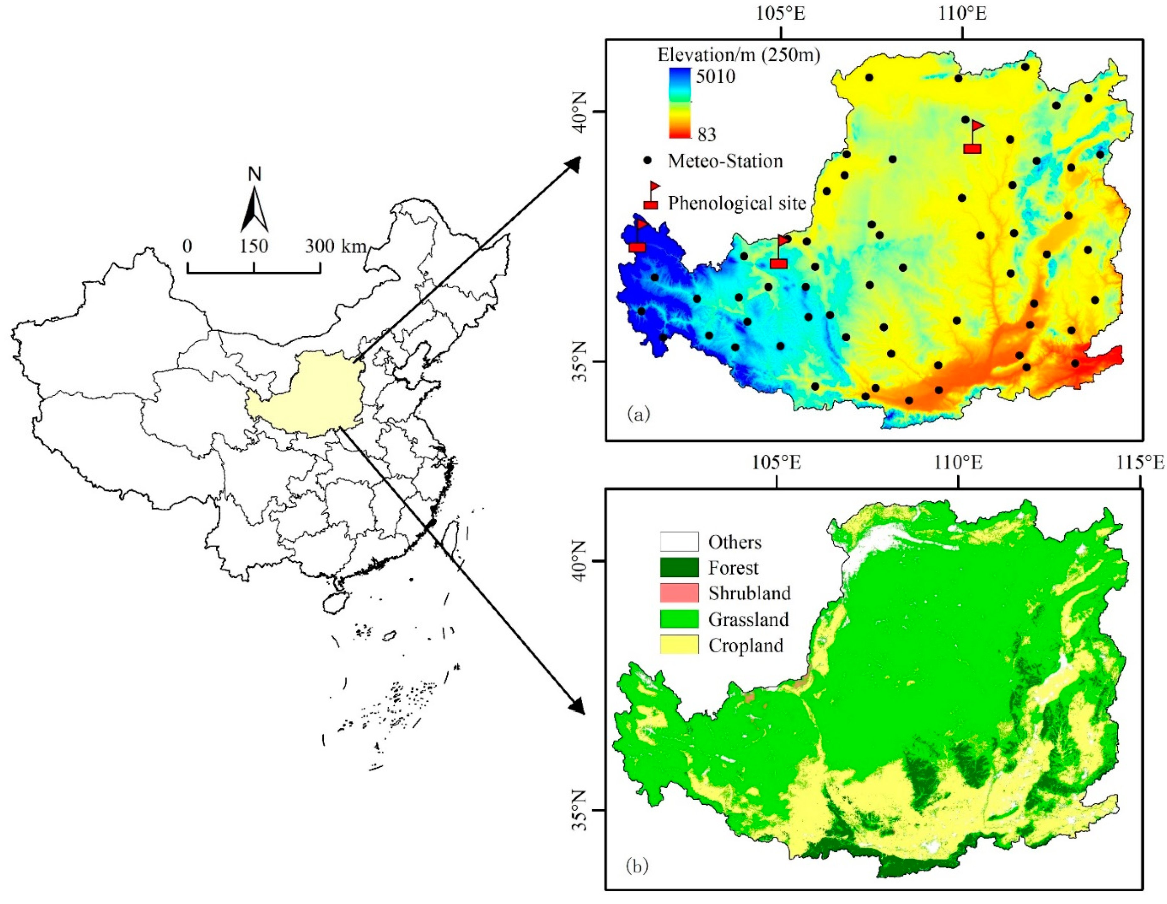
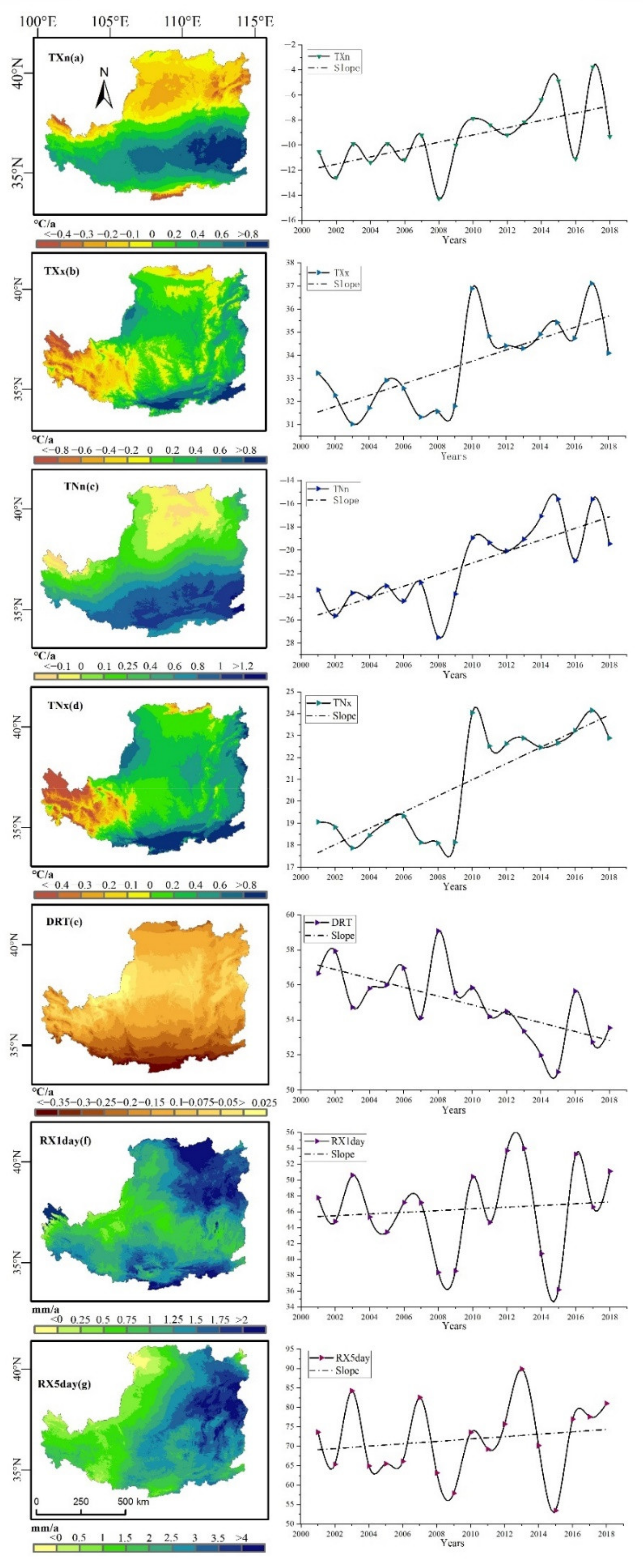
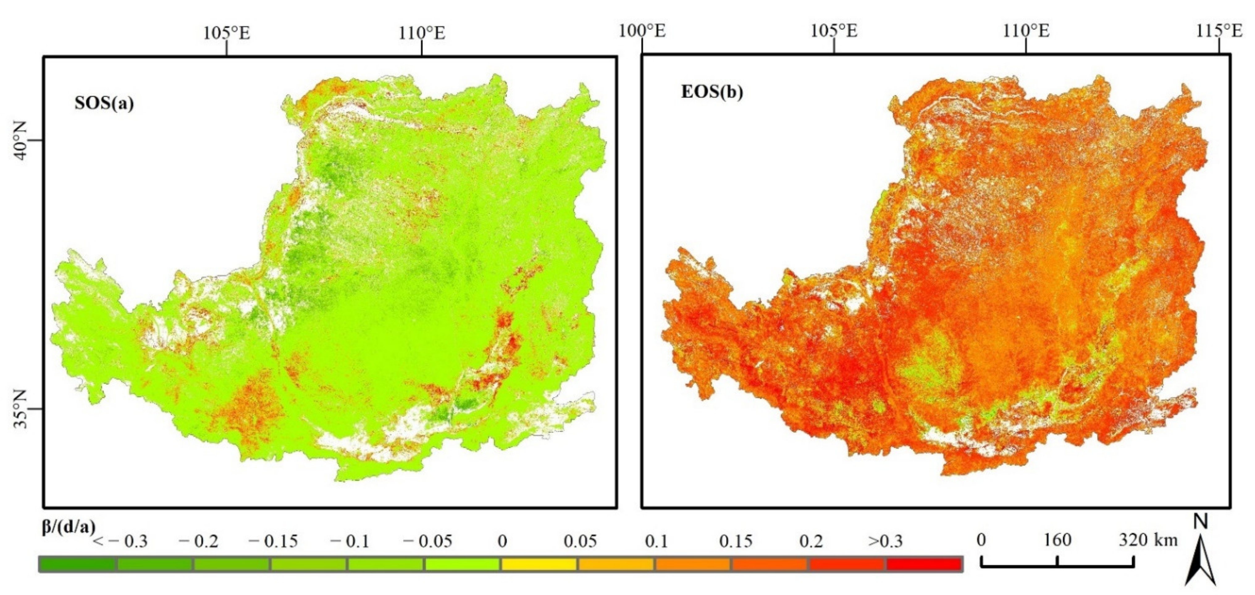
The Loess Plateau is located in the arid and semi-arid region of Northwest China, with a fragile ecological environment and pronounced sensitivity to climate change, so it is very important to study the response of the Loess Plateau to climate indices [18]. Previous scholars quantified the phenology of the Loess Plateau based on different types of data and found that the advancement of vegetation SOS and delay of vegetation EOS on the Loess Plateau in recent years were jointly regulated by mean temperature and total annual precipitation [19,20]. Recent studies have pointed out that there is a significant correlation between the normalized difference vegetation index (NDVI) and extreme temperature index in the Loess Plateau region [21]. However, these studies were either limited to the study of mean climate effects on phenology or to the analysis of vegetation response to climate extremes, whereas the sensitivity of vegetation community-scale phenological changes to extreme climates has been rarely studied at the Loess Plateau. The Loess Plateau forms an obvious environmental gradient with its unique geographical conditions. 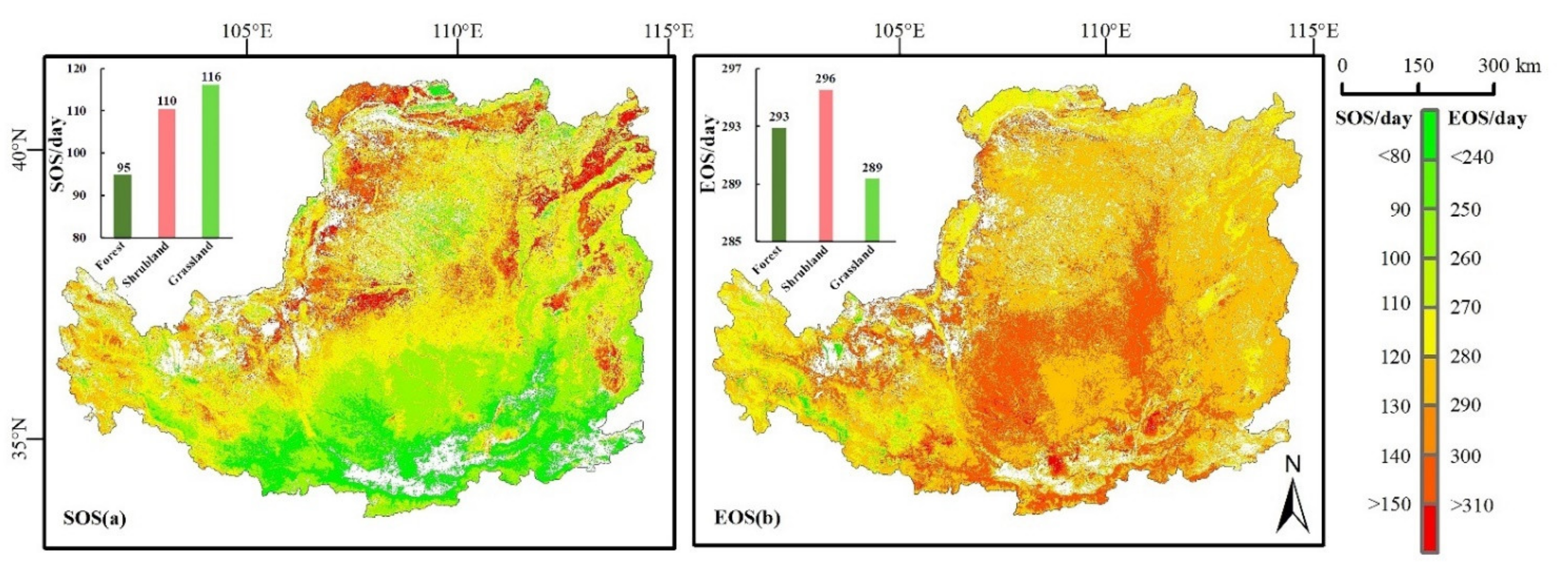Most studies have shown that the total annual precipitation, annual average temperature, and extreme precipitation indices of the Loess Plateau show a decreasing trend from southeast to northwest [3,18,22]. The resulting spatial heterogeneity of energy and water distribution also leads to a distinctive distribution pattern of vegetation, which is low in the northwest and high in the southeast, with the transition from northwest to southeast being mainly from grassland to forest. Therefore, it is important to understand the key factors regulating vegetation phenology and the response of different vegetation types to extreme events in arid and semi-arid areas.

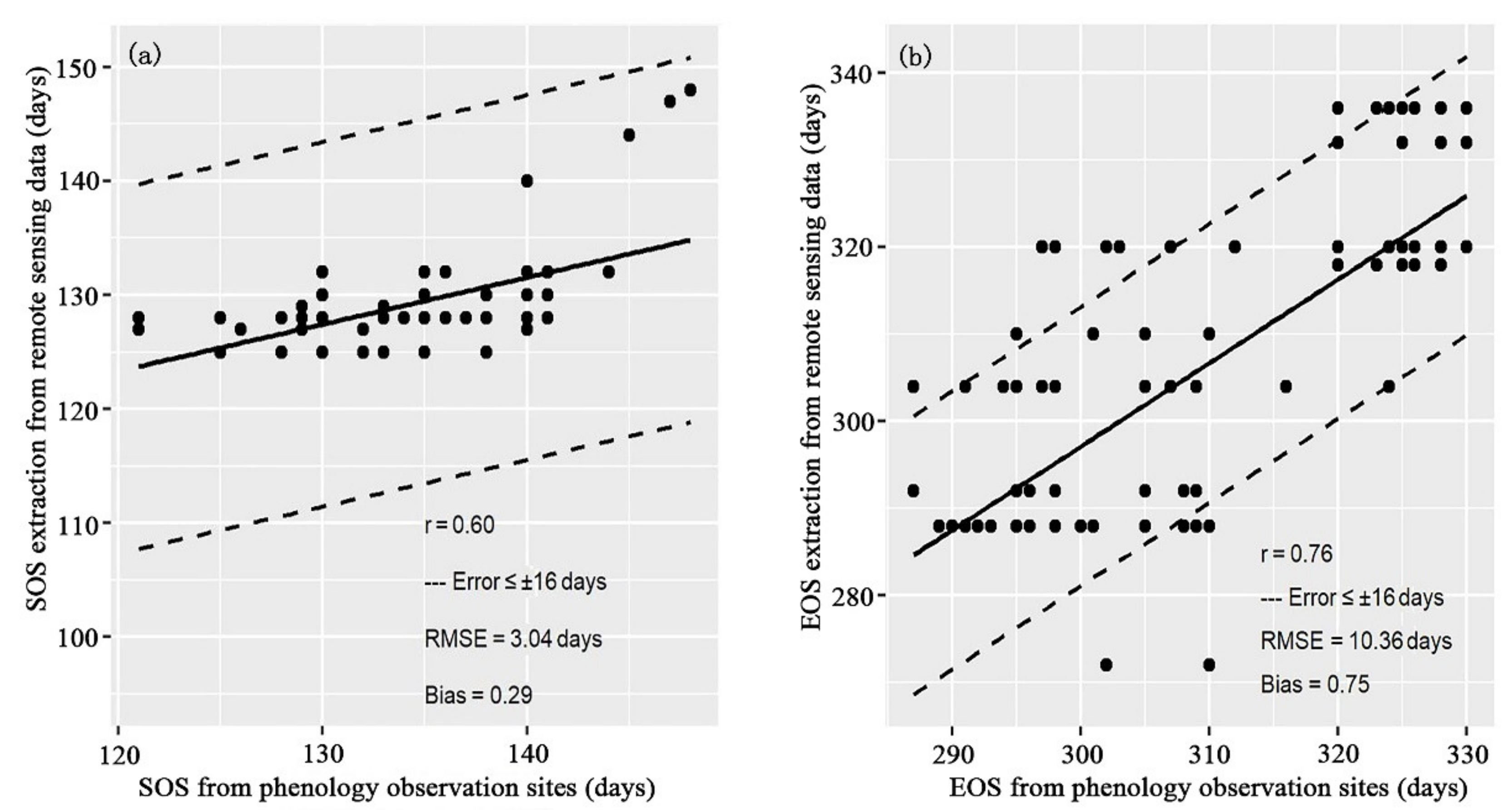
In this study, we mainly used the SOS and EOS data from 2001 to 2018 and seven extreme climate indices to analyze the spatial differentiation of different vegetation phenology’s sensitivities to climate indices. The purpose of this study was to analyze the temporal and spatial changes in vegetation phenology, the spatial and temporal changes of extreme climate indices, and the sensitivity of the response of vegetation phenology to climate extremes. The present study will provide a scientific basis for local response to extreme climate events, disaster prevention and mitigation, and ecological environment protection.

2. Materials and Methods

2.1. Study Area

The Loess Plateau is located in the northwest of China (100°–115° E, 33°– 42° N), with an elevation of 83–5010 m. It is the largest area of loess in the world, characterized by rich, dust-like soil. The topography of the Loess Plateau is high in the northwest and low in the southeast. Due to the multiple constraints of longitude, latitude, and topography, the climate is transitional from the humid monsoon climate in the southeast to the arid climate in the northwest. The winter is cold, dry, and windy, whereas the summer and fall are hot and rainy. The annual average temperature is 3.6–14.3 °C, the annual total precipitation is 300–800 mm, and the precipitation decreases from the southeast to the northwest. Under the influence of climate, the vegetation shows a horizontal zonal distribution from southeast to northwest [19] (Figure 1b). The main vegetation types are forest, shrubland, grassland, and cropland, of which grassland areas for 65%, cropland areas account for 24.20%, forest areas for 6.18%, and shrubland areas for 0.32%. The research described in this article mainly studies forest, shrubland, and grassland.

2.2. Data Sources

The normalization difference vegetation index (NDVI) was used to extract vegetation phenological parameters (https://lpdaacsvc.cr.usgs.gov/appeears, accessed on 23 February 2020). NDVI was derived from the MODIS land cover dynamic product (MOD13Q1) of the National Aeronautics and Space Administration (NASA), with a spatial resolution of 250 m and a temporal resolution of 16 d, over a time period from January 2001 to December 2019. In this paper, the Savitzky–Golay fit (S–G) global filtering method was adopted for 16-d maximum synthetic NDVI data fitting, with NDVI_mean = 0.05 being used as the threshold to exclude non-vegetation coverage.

Phenological validation data come from the National Ecological Science Data Center (http://rs.cern.ac.cn/order/myDataOrders, accessed on 11 January2020), including phenological observation data from the Shapotou, Ordos, and Haibei Stations (Figure 1), which monitor the vegetation for the germination, flowering, seed setting, seed dispersal, and leaf yellowing stages.

The climate data were derived from the daily dataset value from the China Meteorological Data Network (http://data.cma.cn, accessed on 15 January 2020) over the period time of 2000–2018. Previous studies have pointed out that the change of climate conditions in autumn and winter of the previous year will produce hysteresis and accumulation effect to the following year’s vegetation growth [23,24,25]. The period the accumulation effect is 5 to 10 months, and the period the hysteresis effect is 2–3 months [24]. In addition, considering that the vegetation EOS in the Loess Plateau mainly occurs from early September to early October, the extreme climate determined in this study is from September 1 of the previous year to August 31 of the current year [23]. The selected data were first quality-controlled according to RclimDex, and 60 meteorological sites in the study area were selected (Figure 1). Then, the common climate indices recommended by the Expert Team on Climate Change Detection and Indices (ETCCDMI) were used to select the seven climate indices defined in

Table 1. The definitions and classifications of climate indices.

Indicators.	ID	Indicator Name	Definitions	Units
Temperature	TXx	Max Tmax	Yearly maximum value of daily maximum temperature	°C
	TXn	Min Tmax	Yearly minimum value of daily maximum temperature	°C
	TNn	Min Tmin	Yearly minimum value of daily minimum temperature	°C
	TNx	Max Tmin	Yearly maximum value of daily minimum temperature	°C
	DTR	Diurnal temperature range	Yearly mean difference between maximum temperature and minimum temperature	°C
Precipitation	RX1day	Maximum one-day precipitation	Yearly maximum consecutive one-day precipitation	mm
	RX5day	Maximum five-day precipitation	Yearly maximum consecutive five-day precipitation	mm

. The aim was to reflect the marginal state of temperature events and the extreme state of precipitation events [3,26]. The interannual time series of each index was calculated by RclimDex and MATLAB software, and the annual scale data were interpolated into a data set with a spatial resolution of 250 m by ANUSPLINE.

The land-use cover data came from the MODIS land-use cover map (MCD12Q1) provided by NASA (https://lpdaacsvc.cr.usgs.gov/appeears, accessed on 23 February 2020). The spatial resolution of the data was 500 m, and the period was 2001–2018. This article only extracts the areas where the land-use cover types did not change from 2001 to 2018 were extracted.

2.3. Phenological Extract

Because the NDVI image synthesized by maximum value composite (MVC) is greatly affected by cloud and atmosphere, it is necessary to reduce the noise and smooth the image. The NDVI time-series data filtered by the S–G filter method can remove abnormal points and local mutation points and trends and is not limited by the time and space scale of the data and the sensor. This method is determined based on the following equation:

$${\mathrm{Y}}_{\mathrm{j}}=\frac{{\displaystyle {\sum }_{\mathrm{i}=-\mathrm{m}}^{\mathrm{i}=\mathrm{m}}{\mathrm{C}}_{\mathrm{i}}{\mathrm{Y}}_{\mathrm{i}+\mathrm{j}}}}{\mathrm{N}}$$

(1)

where ${\mathrm{Y}}_{\mathrm{j}}$ are the fitted sequence data, $\mathrm{i}$ is for each scene, ${\mathrm{Y}}_{\mathrm{i}+\mathrm{j}}$ are the original sequence data, ${\mathrm{C}}_{\mathrm{i}}$ is the coefficient for the ith NDVI value of the filer, $\mathrm{N}$ is the number of the convoluting integers and is equal to the smoothing window size ($2\mathrm{m}+1$), where $\mathrm{m}$ is the half-width of the smoothing window [27].

Phenology phase extraction methods often include the threshold method, the moving average method, the maximum ratio method, and so on. Considering the scope of the study area and the characteristics of the NDVI changes, analysis this paper is based on the dynamic threshold method proposed by White et al. to calculate and extract the phenological information of NDVI in 2001–2019 on the grid point [28]. The dynamic thresholds of vegetation SOS and vegetation EOS were set at 20% and 80%, respectively, based on the information related to the phenology recorded in the field and based on repeated experiments. Since the TIMESAT 3.2 software can only n−1 year of phenological parameters from n years of data, this paper ultimately obtained the phenology data from 2001 to 2018.

$$\mathrm{N}\mathrm{D}\mathrm{V}{\mathrm{I}}_{\mathrm{ratios}}=\frac{\mathrm{N}\mathrm{D}\mathrm{V}\mathrm{I}-\mathrm{N}\mathrm{D}\mathrm{V}{\mathrm{I}}_{\mathrm{m}\mathrm{i}\mathrm{n}}}{\mathrm{N}\mathrm{D}\mathrm{V}{\mathrm{I}}_{\mathrm{m}\mathrm{a}\mathrm{x}}-\mathrm{N}\mathrm{D}\mathrm{V}{\mathrm{I}}_{\mathrm{m}\mathrm{i}\mathrm{n}}}$$

(2)

where $\mathrm{N}\mathrm{D}\mathrm{V}{\mathrm{I}}_{\mathrm{ratios}}$ are the dynamic thresholds, and $\mathrm{N}\mathrm{D}\mathrm{V}{\mathrm{I}}_{\max }$ and $\mathrm{N}\mathrm{D}\mathrm{V}{\mathrm{I}}_{\min }$ are, respectively, the maximum and minimum NDVI values of the annual NDVI. The date on which the NDVI first exceeds the threshold is defined as the SOS, and the date on which the NDVI first falls below the threshold is defined as the EOS.

In addition, this research assessed the observed phenological data from the phenological sites at the three ground stations (Figure 1). The ground-observed phenological periods were observed at the individual plant scale. To increase the stability of the validation data, records with a record time more than 30 d away from the rest of the data were excluded, according to the study of Hou et al. [29]. The germination period and yellow blight period of the data from three ground observation stations were defined as the vegetation SOS and EOS, respectively.

2.4. Trend Analysis

The direction of the event trend and the slope of the extreme climate index were analyzed by univariate linear regression analysis, and the spatial change trend of vegetation phenology and climate indices were analyzed by Sen’s slope and Mann–Kendal (MK) estimation method [30,31].

2.5. Sensitivity Analysis

The importance of each variable in the Random Forest regression model was used to rank the effects of the seven climate indices on vegetation phenology. The model used the percentage increase in the mean square error (%Inc MSE) to evaluate the influence of each independent variable on the dependent variables [15]. First, the Ntree (number of decision trees) of the decision tree model was constructed, and the out-of-bag (OOB) mean square error of random substitution was calculated, which is recorded as $\mathrm{M}\mathrm{S}{\mathrm{E}}_{11},\mathrm{M}\mathrm{S}{\mathrm{E}}_{12},\cdots ,\mathrm{M}\mathrm{S}{\mathrm{E}}_{\mathrm{m}\mathrm{n}\mathrm{t}\mathrm{r}\mathrm{e}\mathrm{e}}$, as in the following matrix:

$$\left[\begin{array}{cccc}\mathrm{M}\mathrm{S}{\mathrm{E}}_{11}& \mathrm{M}\mathrm{S}{\mathrm{E}}_{12}& \cdots & \mathrm{M}\mathrm{S}{\mathrm{E}}_{1\mathrm{n}\mathrm{t}\mathrm{r}\mathrm{e}\mathrm{e}}\\ \mathrm{M}\mathrm{S}{\mathrm{E}}_{21}& \mathrm{M}\mathrm{S}{\mathrm{E}}_{22}& \cdots & \mathrm{M}\mathrm{S}{\mathrm{E}}_{2\mathrm{n}\mathrm{t}\mathrm{r}\mathrm{e}\mathrm{e}}\\ ⋮& ⋮& ⋮& ⋮\\ \mathrm{M}\mathrm{S}{\mathrm{E}}_{\mathrm{m}1}& \mathrm{M}\mathrm{S}{\mathrm{E}}_{\mathrm{m}2}& \cdots & \mathrm{M}\mathrm{S}{\mathrm{E}}_{\mathrm{m}\mathrm{n}\mathrm{t}\mathrm{r}\mathrm{e}\mathrm{e}}\end{array}\right]$$

(3)

The importance score was calculated as follows:

$$\mathrm{s}\mathrm{c}\mathrm{o}\mathrm{r}\mathrm{e}{\mathrm{X}}_{\mathrm{j}}={\mathrm{S}}_{\mathrm{E}}^{-1}\frac{{\displaystyle {\sum }_{\mathrm{r}=1}^{\mathrm{n}\mathrm{t}\mathrm{r}\mathrm{e}\mathrm{e}}\mathrm{M}\mathrm{S}{\mathrm{E}}_{\mathrm{r}}-\mathrm{M}\mathrm{S}{\mathrm{E}}_{\mathrm{p}\mathrm{r}}}}{\mathrm{n}\mathrm{t}\mathrm{r}\mathrm{e}\mathrm{e}}, (1\le \mathrm{p}\le \mathrm{m})$$

(4)

where n is the number of original data samples and m is the number of variables.

Because ridge regression can eliminate the collinearity between independent variables and eliminate the unbiased nature of the least-squares method, it is widely used in the actual regression process as an improved least squares estimation method. In this research, ridge regression was used to explore the sensitivity of phenology to climate indices. The basic principle is as follows:

$${\widehat{\mathsf{\beta }}}_{\mathrm{R}\mathrm{R}}=({\mathrm{X}}^{\prime }\times \mathrm{X}+\mathrm{k}\times \mathrm{I})\times {\mathrm{X}}^{\prime }$$

(5)

where $\mathrm{X}$ is the observation matrix of the independent variable, $\mathrm{k}$ is the ridge parameter, $\mathrm{I}$ is the identity matrix, and ${\widehat{\mathsf{\beta }}}_{\mathrm{R}\mathrm{R}}$ is the sensitivity coefficient of the independent variable on the dependent variable [32].

3. Results

3.1. Spatial and Temporal Variation Characteristics of Extreme Climate Indices

The temporal trends of extreme climate indices are depicted in Figure 2. The slope of the diurnal temperature range (DRT) index fell at a rate of −2.5 °C/10a, whereas the temperature indices Max Tmax (TXx), Max Tmin (TNx), Min Tmax (TXn), and Min Tmin (TNn) increased at the rates of +2.4 °C/10a, +3.7 °C/10a, +2.9 °C/10a, and +5.0 °C/10a, respectively. Overall, the temporal trends indicate consistent warming. The slopes of the temperature indices, TXn and TNn, were higher than those of TXx and TNx, which further indicates that the climate is warming year by year, whereas the annual difference is decreasing year by year. The precipitation indices maximum one-day precipitation (RX1day) and maximum five-day precipitation (RX5day) increased by +1.1 mm/10a and +23.3 mm/10a, respectively.

The spatial distribution trend of extreme climate indices is depicted in Figure 2. From the perspective of temperature indices, DRT mainly changes in the range −0.02 to −5.7 °C/10a, with the overall region showing a gradually decreasing trend from north to south, with the decreasing trend being obvious in the north. The spatial trends of the TXn and TNn indices were roughly the same, with regional changes of −8.1 to −10.3 °C/10a and −3.8 to −14.4 °C/10a, respectively. There was a shallow trend in the south and a steep trend in the north, with an obvious separating line between the trend differences. The spatial trends of TXx and TNn indices were similar, with variations of −13.5 to −13.8 °C/10a and −15.6 to −11.6 °C/10a across the region, respectively. The western part of the Loess Plateau showed a downward trend, whereas the other regions showed an increasing trend. From the perspective of precipitation indices, RX1day varied from −1.6 mm/10a to +1.0 mm/10a, with an increasing trend in the west and central parts of the Loess Plateau. RX5day changes from −25.7 mm/10a to +37.2 mm/10a, showing an increasing trend from northwest to southeast.

3.2. Temporal and Spatial Variation Characteristics of Vegetation Phenology

As shown in Figure 3, the correlation coefficient between the vegetation SOS identified by remote sensing and the ground-measured vegetation SOS was 0.60 (p < 0.05), and the bias was 0.29. The correlation coefficient between the vegetation EOS identified by remote sensing and the vegetation EOS measured on the ground was 0.76 (p < 0.05), and the bias was 0.75. Except for individual observation data, the error between vegetation phenology by remote sensing and observation data was basically within 16 days. Considering the temporal resolution of the remotely sensed images, these errors are still within acceptable limits. The verification results show that the extracted phenological parameters have high reliability and can reflect the basic characteristics of phenology in this region.

From 2001 to 2018, the vegetation SOS of the Loess Plateau was mainly concentrated in the 96–144 d period (pixels accounted for 90.8%), and the SOS gradually advanced with the topography from northwest to southeast (Figure 4), with the slope of change −0.38 d/a (Figure 5). The SOS of the three vegetation types, namely forest, shrubland and grassland, varied from early to late, respectively. Among them, the forest SOS was mainly concentrated in 80–100 d period, and the shrub and grassland SOS was mainly concentrated in the 90–130 d period, with the area proportion of forest, shrubland and grassland being 90.7%, 80.5%, and 82.5%, respectively (

Table A1. Percentage statistics of average vegetation phenology pixels on the Loess Plateau.

	Forest	Shrubland	Grassland
SOS (80–100d/90–130d)	90.71%	80.54%	82.54%
EOS (280–310d)	98.09%	98.52%	86.92%

). According to Sen’s trend spatial analysis method (Figure 6), most of the pixels of each vegetation type in the study area showed an advancing trend; the percentage of image elements that passed the Mann–Kendall (MK) trend test was 71.0%. The overall study area was 0–1 d/10a earlier, and the pixels of the forest, shrubland, and grassland vegetation accounted for 99.4%, 78.6%, and 81.0%, respectively (

Table A2. Percentage statistics of vegetation phenological trends on the Loess Plateau.

	Forest	Shrubland	Grassland
SOS (0–1 d/10a)	99.41%	78.61%	80.97%
EOS (1–2 d/10a)	78.81%	65.36%	59.36%

), and forest phenology was significantly earlier than shrubland or grassland vegetation. The SOS advancing trend exhibited by grassland was the most obvious, whereas the SOS delay trend of shrubland vegetation was the most obvious.

From 2001 to 2018, the vegetation EOS of the Loess Plateau was mainly concentrated in the period 288–304 d (pixels accounted for 87.0%), and there was little difference in phenological parameters among different vegetation types (Figure 4), with the slope of change being +2.83 d/a (Figure 5). Forest, shrubland and grassland vegetation was mainly concentrated in the period 280–310 d, and their pixel ratios were 98.0%, 98.5%, and 86.9%, respectively (Table A1). According to Sen’s trend space analysis (Figure 6), there was a delayed phenomenon (the percentage of image elements that passed the MK trend test was 75.6%), with the overall delay being 1–3 d/10a. Forest, shrubland, and grassland accounted for 78.8%, 65.4%, and 59.4% of the 1–2 d/10a, respectively (Table A2). The EOS delay trend of the three vegetation types, from small to large, was in the order shrubland > forest > grassland vegetation.

3.3. Effects of Extreme Climate on Vegetation Phenology

3.3.1. The Importance of Extreme Climate Indices to Different Vegetation Phenology Variables

The Random Forest regression model can change the value of a variable into a random number, with larger values indicating the greater importance of the variable. The model was used here to determine the effect of the seven extreme climate indices (Table 1) on different vegetation phenology parameters in the Loess Plateau, focusing on the response of forest, shrubland, grassland, and overall regional vegetation phenology to extreme climate indices (Figure 7).

The importance of different extreme climate indices to changes in different vegetation phenology parameters varied. For SOS, forest phenology was mainly affected by the TXn and DRT indices, whereas shrubland phenology was affected more by the TNn and TXx indices, but the phenology of both vegetation types was greatly affected by extreme temperature indices. Grassland phenology was mainly affected by the DRT and TXx indices. However, the phenology of the overall regional vegetation area was strongly influenced by TNn and TXx, resembling the effect of climate indices on the shrubland phenology. For EOS, forests were mainly influenced by the DRT, TXn, and TNn indices, whereas shrubland was most responsive to RX5day, followed by TNn, with grassland being most affected by TNx and RX1day indices. However, the overall regional vegetation EOS was mainly influenced by the indices TNn, RX5day, and RX1day.

The SOS of different vegetation types was mainly influenced by extreme temperature indices, especially TXx and TNn. EOS values from different vegetation types were not only sensitive to the TNn index but were also influenced by extreme precipitation indices. Therefore, TXx, TNn, DRT, and RX5day are selected as the four extreme climate indices for the subsequent ridge regression sensitivity analysis, based on the importance to vegetation phenology of the seven climate indices (Table 1).

3.3.2. Sensitivity Analysis of Phenology to Extreme Climate Indices

The spatial distribution of phenology sensitivity to the extreme climate indices TXx, TNn, DRT, and RX5day in the Loess Plateau from 2001 to 2018 was assessed (Figure 8;

Table A3. Percentage statistics of significant pixels of SOS sensitivity to the extreme climate index on the Loess Plateau.

	DRT	TXX	TNN	PRE5
Significant	4.68%	5.09%	7.69%	8.83%
Nonsignificant	95.32%	94.91%	92.31%	91.17%

and

Table A4. Percentage statistics of significant pixels of EOS sensitivity to extreme climate index on the Loess Plateau.

	DRT	TXX	TNN	PRE5
Significant	8.68%	7.04%	3.98%	9.04%
Nonsignificant	91.32%	92.96%	96.02%	90.96%

). Vegetation phenology showed different spatial differentiation with respect to the four climate indices. Except for the negative sense of the overall phenology to the DRT index, the phenology measures SOS and EOS showed opposite spatial distributions to indices TXx, TNn, and RX5day. The sensitivity coefficient of SOS was positive, whereas that of EOS was negative. The RX5day index showed an overall positive sensitivity coefficient for SOS and an overall negative sensitivity coefficient for EOS (Figure 8d,h). The regions with positive sensitivity to the hot, extreme temperature index, TXx, showed negative sensitivity to the cold, extreme temperature index, TNn. The SOS parameter, γ_TXx, was negative in the western part of the Loess Plateau and positive in the northeastern part, whereas γ_TNn showed the opposite distribution (Figure 8a,b). The EOS parameter, γ_TXx, was negative in the western part of the Loess Plateau and positive in the southern part, whereas γ_TNn showed the opposite trend (Figure 8e,f). The sensitivity coefficients of phenology to temperature indices were significantly higher than those of the precipitation indices, and the sensitivity coefficients of the TXx and DRT indices were higher than that of the TNn index.

In addition, the sensitivity of the phenology of different vegetation to climate indices TXx, TNn, DRT, and RX5day was compared and analyzed (Figure 9). We found that the sensitivity of EOS to each climate index was significantly higher than that of SOS, indicating that the change in each unit of climate index caused a greater change in the EOS than that of the SOS. The sensitivity of the phenology of the three vegetation types to the DRT index was the highest (

Table A5. Significant sensitivity of phenology of different vegetation types to extreme climate indices on the Loess Plateau.

	SOS			EOS
	Forest	Shrubland	Grassland	Forest	Shrubland	Grassland
DRT	0	0.04	0.01	0.24	0.58	0.86
RX5day	0	0.55	0.79	0.22	0.19	0.39
TNn	0.02	0.68	0.02	0.57	0.32	0.71
TXx	0.94	0.27	0	0.88	0.86	0.61

), and the sensitivity coefficients were all negative. Comparing the sensitivity of the phenology of the three kinds of vegetation to climate index in the spring, it was found that the sensitivity of shrubland and grassland to climate indices was greater than that of the forest, indicating that the stability of the forest was greater than that of shrubland and grassland, with the γ_TNn, γ_DRT, and γ_RX5day values for shrubland in spring being higher than those of forest and grassland. Comparing the sensitivity of the phenology of the three vegetation types to climate indices the fall, we found that γ_TNn and γ_RX5day values were greater in the fall in the forest than at the same season in shrubland and grassland. Comparing the sensitivity of phenology of the three vegetation types to climate indices in the fall, we found that γ_TNn and γ_RX5day were higher in the fall in the forest than in shrubland or grassland (p < 0.01; Table A5). In response to RX5day, forest phenology will end the growing season early in the fall. Compared with other climatic indexes, fall shrubland phenology is the one most sensitive to the TXx index. The fall grassland parameter γ_TXx was higher than that of forest or shrubland, indicating that the fall grassland phenology was influenced by the TXx index to end the growing season the latest of the three vegetation.

4. Discussion

The Loess Plateau is the largest loess region on the earth. Its climate is characterized by drought, little rain, strong wind, and more sand, which leads to dusty and sandy weather in this region and its surrounding areas [33]. 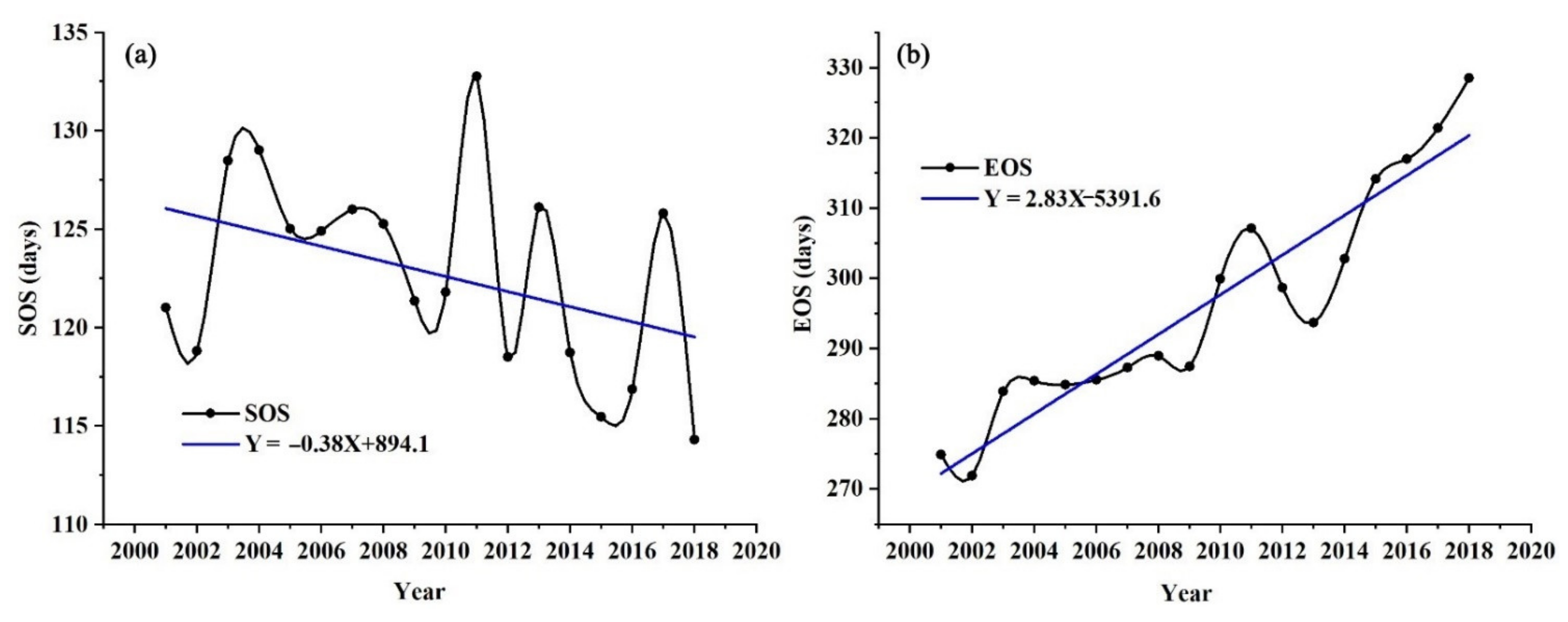In the past two decades, the government of the People’s Republic of China has taken a series of measures to improve its fragile ecological environments, such as returning farmland to forest, sealing sand for forest and grass cultivation, and vegetation coverage has been effectively improved [34]. This paper indicates clearly that SOS advanced and EOS delayed, and the growth period of the whole vegetation showed an increasing trend. Moreover, in the context of climate change (increasing temperature, increasing precipitation, and frequent extreme events), vegetation phenology on the Loess Plateau has undergone significant changes [19], and phenology also affects climate change to a certain extent [35]. For example, when Chang et al. [36] studied the relationship between the frequency of sandstorm and air humidity as well as plant phenology in the Minqin desert area, they believed that the wet and warm climate, vegetation SOS advance, and vegetation EOS delay could reduce the frequency of sandstorm days.

Most studies have shown that extreme climate events have an impact on vegetation phenology. Extreme temperature events affect the growth and development of vegetation through effects on the activities of photosynthetic and respiration enzymes [15,37]. Extreme precipitation events restrict growth by affecting the water content or availability in the soil in which the vegetation is growing [38]. Piao et al. found that vegetation in northern areas was more affected by high temperatures than by precipitation [39]. Through experimentation, Nagy et al. found that phenology was affected by extreme climate indices [13], observing that the flowering date of temperate vegetation was nearly one month earlier, and some vegetation species could not complete their flowering cycles, but the phenology of the vegetation studied was not affected by heavy precipitation events.

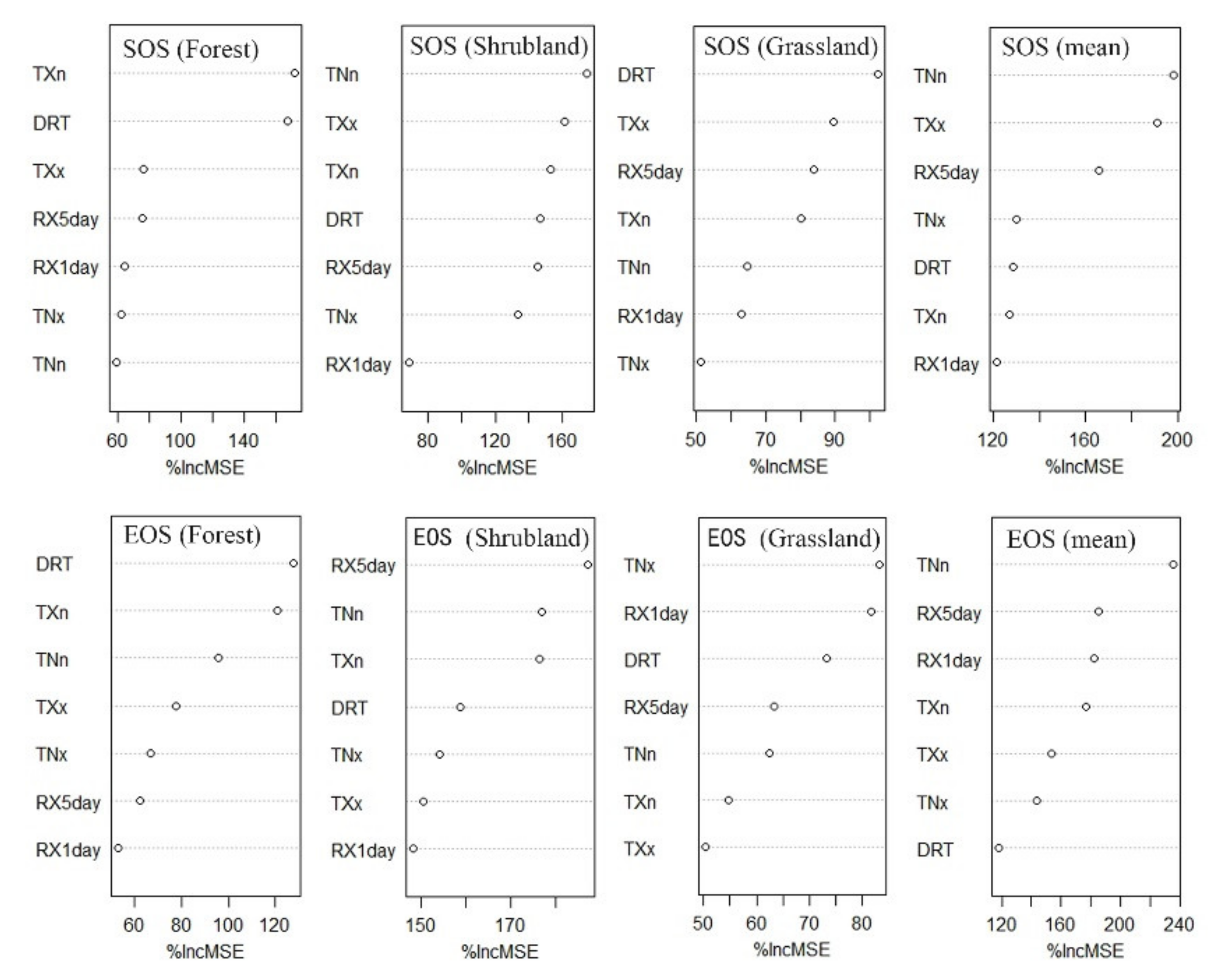
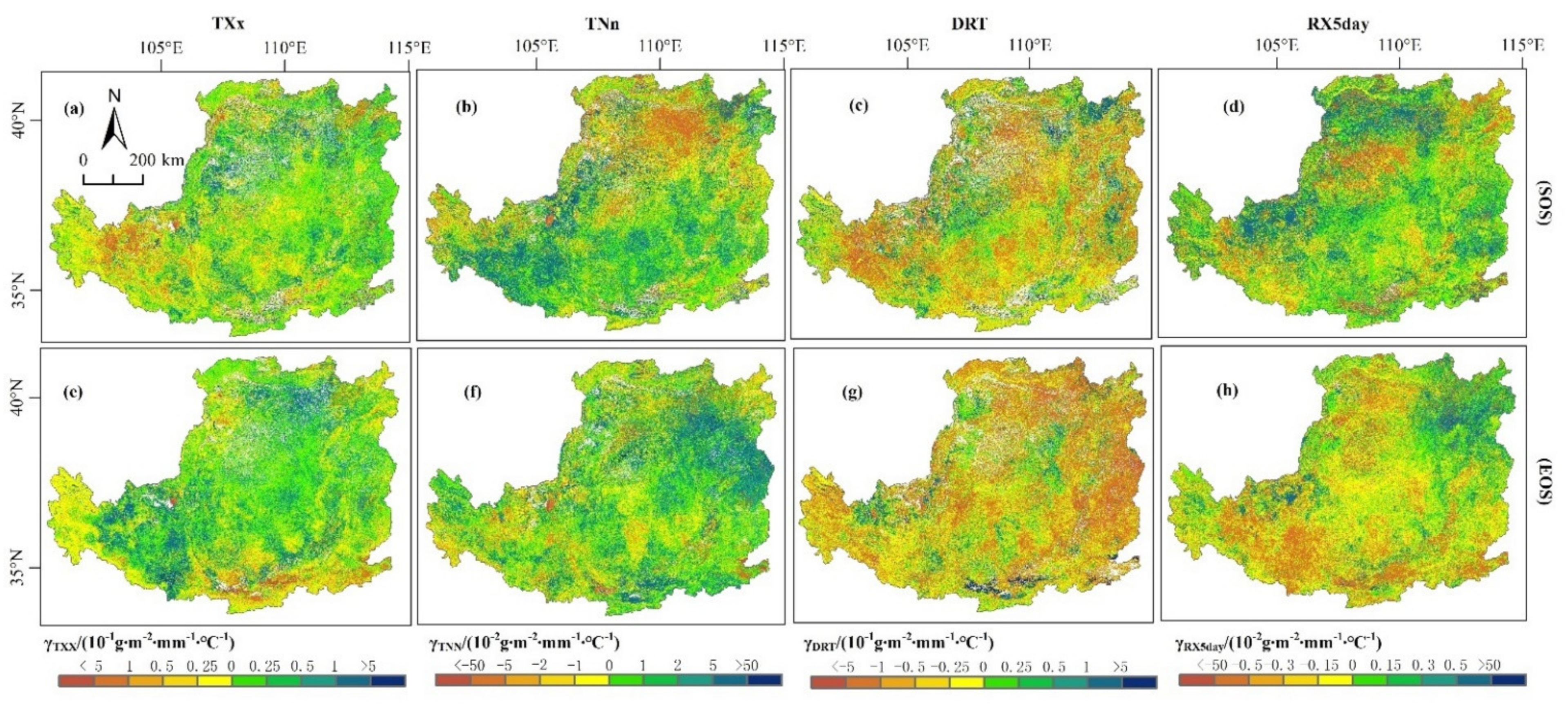
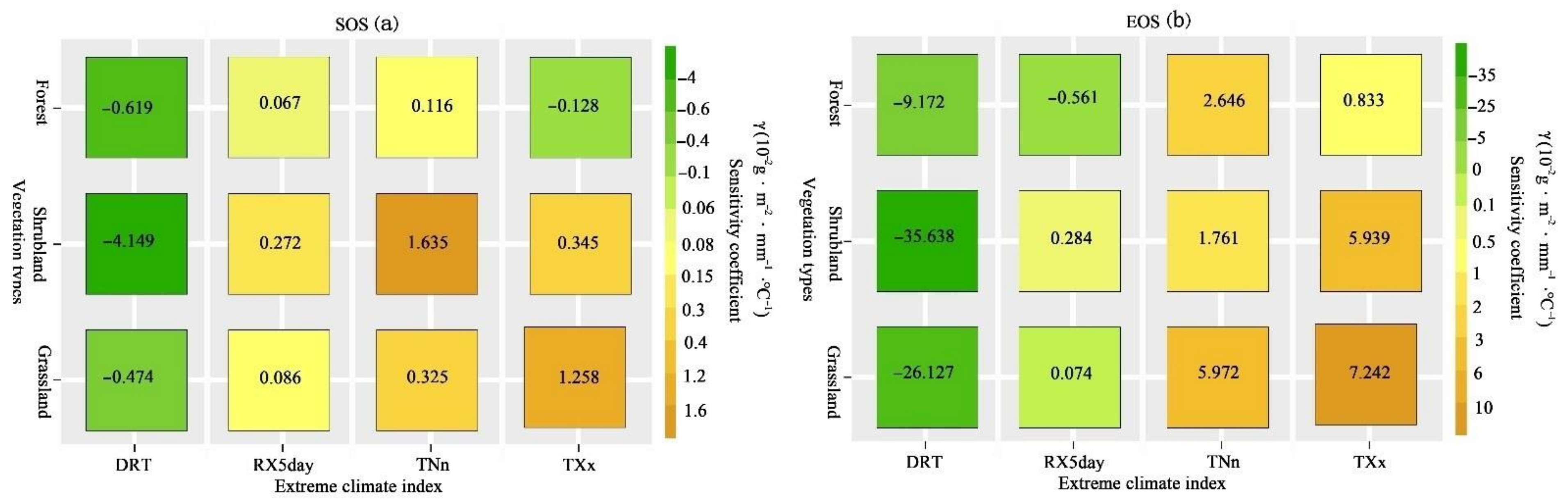
In the current study, we found that both extreme temperature events and extreme precipitation events affected vegetation phenology, with the sensitivity of phenology to extreme temperature events being greater than that to extreme precipitation. The possible cause of this finding is that the Loess Plateau is in an arid and semi-arid region. Vegetation has adapted to the extremely dry environment, resulting in a weak relationship between vegetation phenology and extreme precipitation events. Although, to some extent, phenology is affected by heavy precipitation events [15]. Among the three vegetation types studied in this paper, the autumn forest phenology responds to the influence of the RX5day index by ending the early growing season. The possible reason is that forest vegetation sites have soil with higher soil water contents than those sites supporting shrubland and grassland, and further increases in more water input will form an anaerobic environment in the plant rhizosphere, thus preventing the growth of vegetation.

The sensitivity of the response of the phenology of different vegetation types to extreme climate events is complex. We found that the sensitivity of phenology to the DRT index was negative. In other words, when the daily temperature difference causes the advance of vegetation phenology in the spring, it will indirectly lead to the early end of the fall vegetation growing season. The possible reason is that the rates of increase in TXx and TNx indices were higher than those of the TXn and TNn indices in the years under study. Unusual warming events may prematurely induce plant activity, but this situation is not conducive to the growth of vegetation, as it would lead to the subsequent early end of the vegetation growing season, thus shortening the vegetation growth cycle because plants need exposure to lower temperatures before dormancy ends. Another possible reason is that when vegetation encounters environmental stress, its own constantly changing signals, mainly including hormones and signal molecules, will control phenology, namely germination, leaf senescence, and growth stagnation. Vegetation ends its growing season early to avoid damage to itself caused by environmental stress. In addition, the seasonal trajectories of vegetation activities are likely to be more sensitive to extreme climates [40,41].

The high temperatures in the spring of the ecosystem of arid regions in Australia will seriously delay or blocks phenological cycles [42]. Siegmund et al. found that high temperature usually had a strong negative effect on flowering in four shrub species, a finding which was similar to the sensitivity response of spring phenology to extreme temperature [5]. The TNn and TXn indices had a significant delaying effect on fall phenology delay in the Tibetan Plateau, while Hong et al. considered that warm days and warm nights were the main factors affecting the phenological delay of vegetation in the fall [15]. The above results differ from our findings in that fall forest, shrubland, and grassland phenology were all delayed by TXx and TNn indices. Although the evidence that phenology is affected by extreme weather is increasing, with the increasing frequency of extreme events [2], vegetation phenology in sensitive areas is also increasingly affected by it. The focus of future research should become how to deal with the significant impact on ecosystems caused by extreme events.

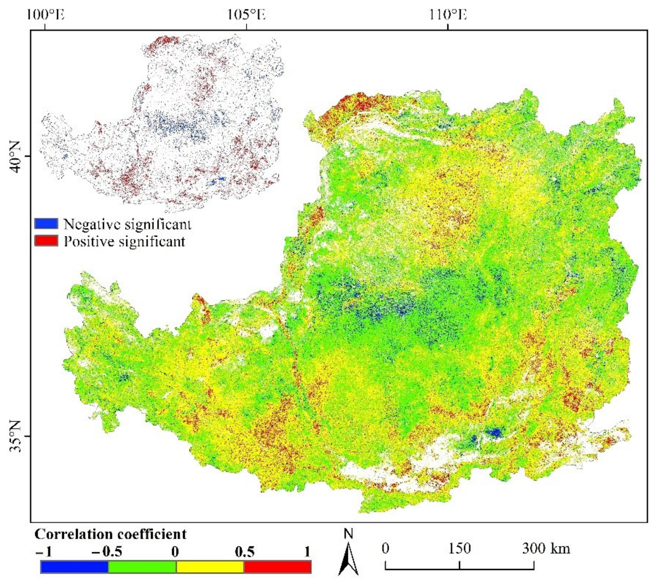
In addition, vegetation phenology is both a periodic and a continuously dynamic process, which is restricted by numerous influencing factors, which interacted with one another [25]. Previous studies have generally believed that climate change is the most important factor affecting vegetation phenology [19,43]. In this current study, we also focused on the phenological change affected by extreme climate indices, but, in the process of analysis, we found that the advance of vegetation SOS by extreme climate indices may indirectly lead to the advance of vegetation EOS; after the vegetation EOS is affected by extreme climate in the current year, it may also lead to changes in vegetation SOS in the following year. Therefore, in this paper, we carried out makes a correlation analysis between vegetation SOS and vegetation EOS. Our results showed that there was a correlation between vegetation SOS and vegetation EOS on the Loess Plateau (Figure 10), with the areas with significant correlations being mainly distributed in the areas with the high correlation coefficients. The reason for this result may be that vegetation needs its own stored carbohydrates and nutrients with one another growth and development, and that delay in vegetation EOS may cause a longer storage period in which to store more reserves [44,45]. These reserves can then be supplied to power shoot development and growth of vegetation in the second year, thus promoting the advance of vegetation SOS [46]. Of course, these explanations are only from the perspective of nutrition. The exact contribution between vegetation SOS and vegetation EOS is difficult to define, and there is no direct evidence to prove any relationship between vegetation SOS and vegetation EOS on the scale of the community ecosystem. Therefore, this is an open question, which requires exploration of the mechanism of the interaction between large-scale vegetation SOS and vegetation EOS and the phenological differences among secondary vegetation types, in combination with remote sensing and vegetation nutrition.

5. Conclusions

The research described in this paper uses the daily maximum and minimum temperature and precipitation data from 60 meteorological stations over the period 2001 to 2018 to analyze seven extreme climatic indices of the Loess Plateau. Based on MOD13Q1 land-use cover map data, this paper analyzes the spatiotemporal patterns and change trends of vegetation phenology in the study area and discusses the influence of climate events and trends on vegetation phenology. The results showed:

• The extreme temperature in the Loess Plateau increased continuously from 2001 to 2018. The rate of increase in the TNn index was higher than that of the TXx index, which is the fundamental reason for the decline of the DRT index. The extreme precipitation index showed an increasing trend, with the precipitation events in the east being higher than those in the west.
• The SOS of vegetation on the Loess Plateau gradually advanced with the topography from the northwest to southeast, with most of the vegetation in the study area showing a trend of an advancing SOS. There was little difference in phenological EOS values among the different vegetation types, with all three types showing a tendency toward a delayed EOS.
• The vegetation phenology on the Loess Plateau showed variation in spatial differentiation in response to different climate indices, with positive sensitivity coefficients between SOS and climate indices, compared with a negative sensitivity coefficient between EOS and climate indices. It means that extreme climate change leading to an advance in vegetation SOS may indirectly lead to an advance in vegetation EOS. This means that extreme climate change, leading to an advance in vegetation SOS, may indirectly lead to an advance in vegetation EOS.
• The sensitivity of the EOS of forest, shrubland, and grassland vegetation to climate index was higher than that of the SOS, with the phenology of all vegetation types being affected by the DRT index. The shrubland SOS was more sensitive to extreme events than the forest and grassland SOS, whereas the grassland EOS was delayed by high temperatures.

References

1. Qin, D.H. Climate change science and sustainable human development. Prog. Geogr. 2014, 33, 874–883. [Google Scholar]
2. IPCC. Climate Change 2013: The Physical Science Basis: The Summary for Policymakers of the Working Group I Contribution to the Fifth Assessment Report; Cambridge University Press: Cambridge, UK, 2013. [Google Scholar]
3. Wang, H.J.; Pan, Y.P.; Li, S.; Chen, Z.S.; Zhao, Z.Y.; Mi, H.X. Risk Assessment and Zonation of Meteorological Disasters Based on Rasterization in Jiangsu Province. J. Liaocheng Univ. Nat. Sci. Ed. 2019, 32, 99–110. [Google Scholar] [CrossRef]
4. Huang, H.; Zhang, B.; Huang, T.; Wang, H.J.; Ma, S.Q.; Ma, B.; Wang, X.D.; Cui, Y.Q. Quantifying and predicting spatial and temporal variations in extreme temperatures since 1990 in Gansu Province, China. Arid Land Geogr. 2020, 43, 319–328. [Google Scholar]
5. Siegmund, J.F.; Wiedermann, M.; Donges, J.F.; Donner, R.V. Impact of temperature and precipitation extremes on the flowering dates of four German wildlife shrub species. Biogeosciences 2016, 13, 5541–5555. [Google Scholar] [CrossRef] [Green Version]
6. Moors, E.J. Influence of spring and autumn phenological transitions on forest ecosystem productivity. Philos. Trans. R. Soc. B Biol. Sci. 2010, 365, 3227–3246. [Google Scholar] [CrossRef] [Green Version]
7. Barichivich, J.; Briffa, K.R.; Osborn, T.J.; Melvin, T.M.; Caesar, J. Thermal growing season and timing of biospheric carbon uptake across the Northern Hemisphere. Glob. Biogeochem. Cycles 2012, 26, 4015. [Google Scholar] [CrossRef]
8. Keenan, T.F.; Gray, J.; Friedl, M.A.; Toomey, M.; Bohrer, G.; Hollinger, D.Y.; Munger, J.W.; O’Keefe, J.; Schmid, H.P.; Wing, I.S. Net carbon uptake has increased through warming-induced changes in temperate forest phenol. Nat. Clim. Chang. 2014, 4, 598–604. [Google Scholar] [CrossRef]
9. Huang, W.J. Alpine Grassland Phenology Response to Climate Change over Tibetan Plateau. Master’s Thesis, Lanzhou University, Lanzhou, China, 2019. [Google Scholar]
10. Piao, S.L.; Tan, J.G.; Chen, A.P.; Fu, Y.H.; Ciais, P.; Liu, Q.; Janssens, I.A.; Vicca, S.; Zeng, Z.Z.; Jeong, S.J.; et al. Leaf onset in the northern hemisphere triggered by daytime temperature. Nat. Commun. 2015, 6, 6911. [Google Scholar] [CrossRef] [Green Version]
11. Nagy, L.; Kreyling, J.; Gellesch, E.; Beierkuhnlein, C.; Jentsch, A. Recurring weather extremes alter the flowering phenology of two common temperate shrubs. Int. J. Biometeorol. 2013, 57, 579–588. [Google Scholar] [CrossRef]
12. Li, P. Dynamics of Vegetation Autumn Phenology and Their Response to Extremely Climate Change in the Qinghai-Tibet Plateau. Ph.D. Thesis, Northwest A&F University, Xianyang, China, 2017. [Google Scholar]
13. Hong, Y.; Zhang, H.Y.; Zhao, J.J.; Shan, Y.; Zhang, Z.X.; Guo, X.Y.; Rihan, W.; Deng, G.R. Effects of spring and summer extreme climate events on the autumn phenology of different vegetation types of Inner Mongolia, China, from 1982 to 2015. Ecol. Indic. 2020, 111, 105974. [Google Scholar] [CrossRef]
14. Bokhorst, S.; Tømmervik, H.; Callaghan, T.V.; Phoenix, G.K.; Bjerke, J.W. Vegetation recovery following extreme winter warming events in the sub-Arctic estimated using NDVI from remote sensing and handheld passive proximal sensors. Environ. Exp. Bot. 2012, 81, 18–25. [Google Scholar] [CrossRef]
15. Xie, Y.Y.; Wang, X.J.; Silander, J.A. Deciduous forest responses to temperature, precipitation, and drought imply complex climate change impacts. Proc. Natl. Acad. Sci. USA 2015, 112, 13585–13590. [Google Scholar] [CrossRef] [Green Version]
16. Ciais, P.; Reichstein, M.; Viovy, N.; Granier, A.; Ogée, J.; Allard, V.; Aubinet, M.; Buchmann, N.; Bernhofer, C.; Carrara, A. Europe-wide reduction in primary productivity caused by the heat and drought in 2003. Nature 2005, 437, 529–533. [Google Scholar] [CrossRef]
17. Cleland, E.E.; Chuine, I.; Menzel, A.; Mooney, H.A.; Schwartz, M.D. Shifting plant phenology in response to global change. Trends Ecol. Evol. 2007, 22, 357–365. [Google Scholar] [CrossRef]
18. Zhao, A.Z.; Zhu, X.F.; Pan, Y.Z. Spatiotemporal variations of extreme precipitation events in the loess plateau from 1965 to 2013. J. Beijing Norm. Univ. Nat. Sci. 2017, 53, 43–50. [Google Scholar] [CrossRef]
19. Xie, B.N.; Qin, Z.F.; Wang, Y.; Chang, R.Q. Monitoring vegetation phenology and their response to climate change on Chinese Loess Plateau based on remote sensing. Trans. Chin. Soc. Agric. Eng. 2015, 31, 153–160. [Google Scholar]
20. Lei, J.; Yao, Y.B.; Sun, R.; Guo, J.P.; Niu, H.Y. Phenological variation and its response to climate warming in semi-arid region of loess plateau. Chin. J. Agrometeorol. 2017, 38, 1–8. [Google Scholar]
21. Han, D.D. Change of Vegetation and Its Response to Extreme Climate in the Loess Plateau. Master’s Thesis, University of Chinese Academy of Sciences, Beijing, China, 2020. [Google Scholar]
22. Zhao, A.Z.; Liu, X.F.; Zhu, X.F.; Pan, Y.Z.; Zhao, Y.L.; Wang, D.L. Trend variations and spatial difference of extreme air temperature events in the loess plateau from 1965 to 2013. Geogr. Res. 2016, 35, 639–652. [Google Scholar]
23. He, Z.B.; Du, J.; Chen, L.F.; Zhu, X.; Lin, P.F.; Zhao, M.M.; Fang, S. Impacts of Recent Climate Extremes on Spring Phenology in Arid-mountain Ecosystems in China. Agric. For. Meteorol. 2018, 260, 31–40. [Google Scholar] [CrossRef]
24. Zhao, A.Z.; Yu, Q.Y.; Feng, L.L.; Zhang, A.B.; Pei, T. Evaluating the cumulative and time-lag effects of drought on grassland. J. Environ. Manag. 2020, 261, 110214. [Google Scholar] [CrossRef]
25. Kong, D.D.; Zhang, Q.; Huang, W.L.; Gu, X.H. Vegetation phenology change in Tibetan Plateau from 1982 to 2013 and its related meteorological factors. Acta Geogr. Sin. 2017, 72, 39–52. [Google Scholar]
26. Frich, P.L.; Alexander, L.V.; Della-Marta, P.M.; Gleason, B.; Peterson, T.C. Observed coherent changes in climate extremes during 2nd half of the 20th century. Clim. Res. 2002, 19, 193–212. [Google Scholar] [CrossRef] [Green Version]
27. Chen, J.; Jonsson, P.; Tamura, M.; Gu, Z.H.; Matsushita, B.; Eklundh, L. A simple method for reconstructing a high-quality NDVI time-series data set based on the Savitzky–Golay filter. Remote Sens. Environ. 2004, 91, 332–344. [Google Scholar] [CrossRef]
28. White, M.A.; Thomton, P.E.; Running, S.W. A continental phenology model for monitoring vegetation responses to interannual climatic variability. Glob. Biogeochem. Cycles 1997, 11, 217–234. [Google Scholar] [CrossRef]
29. Hou, X.H.; Niu, Z.; Gao, S. Phenology of Forest Vegetation in Northeast of China in Ten Years Using Remote Sensing. Spectrosc. Spectr. Anal. 2014, 34, 515–519. [Google Scholar]
30. Theil, H. A Rank-Invariant Method of Linear and Polynomial Regression Analysis; I, II and III; Koninklijke Nederlandse Akademie van Wetenschappen: Amsterdam, The Netherlands, 1950; Volume 53, pp. 386–392, 521–525, 1397–1412. [Google Scholar]
31. Sen, P.K. Estimates of the regression coefficient based on Kendall’s tau. J. Am. Stat. Assoc. 1968, 63, 1379–1389. [Google Scholar] [CrossRef]
32. Walker, E.; Birch, J.B. Influence measures in ridge regression. Technometrics 1988, 30, 221–227. [Google Scholar] [CrossRef]
33. Fu, B.J.; Wang, S.; Liu, Y.; Liu, J.B.; Liang, W.; Miao, C.Y. Hydrogeomorphic ecosystem responses to natural and anthropogenic changes in the loess plateau of china. Annu. Rev. Earth Planet. Sci. 2016, 45, 223–243. [Google Scholar] [CrossRef]
34. Li, T.; Lü, Y.H.; Ren, Y.J.; Li, P.F. Gauging the effectiveness of vegetation restoration and the influence factors in the Loess Plateau. Acta Ecol. Sin. 2020, 40, 8593–8605. [Google Scholar]
35. Lian, X.; Piao, S.L.; Li, L.Z.X.; Li, Y.; Huntingford, C.; Ciais, P.; Cescatti, A.; Janssens, I.A.; Peñuelas, J.; Buermann, W.; et al. Summer soil drying exacerbated by earlier spring greening of northern vegetation. Sci. Adv. 2020, 6. [Google Scholar] [CrossRef] [Green Version]
36. Chang, Z.F.; Wang, Y.L.; Han, F.G.; Zhong, S.N. Relationship between frequency of sandstorms and air humidity as well as plant phenology: A case study from the Minqin desert area. Acta Ecol. Sin. 2012, 32, 1378–1386. [Google Scholar] [CrossRef]
37. Liu, Q.; Fu, Y.H.; Zeng, Z.Z.; Huang, M.T.; Li, X.R.; Piao, S.L. Temperature, precipitation, and insolation effects on autumn vegetation phenology in temperate China. Glob. Chang. Biol. 2016, 22, 644–655. [Google Scholar] [CrossRef] [PubMed]
38. Lupascu, M.; Welker, J.M.; Seibt, U.; Xu, X.; Velicogna, I.; Lindsey, D.S.; Czimczik, C.I. The amount and timing of precipitation control the magnitude, seasonality and sources (14 C) of ecosystem respiration in a polar semi-desert, northwestern Greenland. Biogeosciences 2014, 11, 2457–2496. [Google Scholar] [CrossRef] [Green Version]
39. Piao, S.L.; Fang, J.Y.; Zhou, L.M.; Ciais, P.; Zhu, B. Variations in satellite-derived phenology in china’s temperate vegetation. Glob. Chang. Biol. 2010, 12, 672–685. [Google Scholar] [CrossRef]
40. Butt, N.; Seabrook, L.; Maron, M.; Law, B.S.; Dawson, T.P.; Syktus, J.; McAlpine, C.A. Cascading effects of climate extremes on vertebrate fauna through changes to low-latitude tree flowering and fruiting phenology. Glob. Chang. Biol. 2015, 21, 3267–3277. [Google Scholar] [CrossRef] [Green Version]
41. Crabbe, R.A.; Dash, J.; Rodriguez-Galiano, V.F.; Janous, D.; Pavelka, M.; Marek, M.V. Extreme warm temperatures alter forest phenology and productivity in Europe. Sci. Total. Environ. 2016, 563, 486–495. [Google Scholar] [CrossRef]
42. Ma, X.L.; Huete, A.; Moran, S.; Ponce-Campos, G.; Eamus, D. Abrupt shifts in phenology and vegetation productivity under climate extremes. J. Geophys. Res. Biogeosci. 2015, 120, 2036–2052. [Google Scholar] [CrossRef]
43. Penuelas, J.; Rutishauser, T.; Filella, I. Phenology Feedbacks on Climate Change. Science 2009, 324, 887–888. [Google Scholar] [CrossRef] [Green Version]
44. Han, Q.M.; Kabeya, D. Recent developments in understanding mast seeding in relation to dynamics of carbon and nitrogen resources in temperate trees. Ecol. Res. 2017, 32, 1–8. [Google Scholar] [CrossRef]
45. Lawrence, B.T.; Melgar, J.C. Variable fall climate influences nutrient resorption and reserve storage in young peach trees. Front. Plant Sci. 2018, 9, 1819. [Google Scholar] [CrossRef] [Green Version]
46. Bazot, S.; Fresneau, C.; Damesin, C.; Barthes, L. Contribution of previous year’s leaf N and soil N uptake to current year’s leaf growth in sessile oak. Biogeosciences 2016, 13, 3475–3484. [Google Scholar] [CrossRef] [Green Version]
Figure 1. The geographical location of the Loess Plateau: (a) a topographic map of the Loess Plateau and (b) a vegetation type map of the Loess Plateau. Meteo-Station is Meteorological Station.
Sustainability 13 07623 g001
Figure 2. Spatial (left) and temporal (right) distributions of extreme climate indices on the Loess Plateau from 2001 to 2018. The slopes for the temporal distributions were determined by univariate regression analysis. The indices are (a) TXn, (b) TXx, (c) TNn, (d) TNx, (e) DRT, (f) RX1day, and (g) RX5day.
Sustainability 13 07623 g002
Figure 3. A comparison of phenological results from remote sensing with those from ground observations. Verification of the SOS is (a), Verification of the EOS is (b).
Sustainability 13 07623 g003
Figure 4. Spatial distribution of the annual phenological mean values for the (a) start of the growing season (SOS) and (b) end of the growing season (EOS) of the three vegetation types on the Loess Plateau (2001–2018).
Sustainability 13 07623 g004
Figure 5. Interannual trend variation trend of vegetation phenology measures of the (a) start of the growing season (SOS) and (b) end of the growing season (EOS) on the Loess Plateau from 2001 to 2018.
Sustainability 13 07623 g005
Figure 6. Spatial distribution of phenological change trend of the (a) start of the growing season (SOS) and (b) end of the growing season (EOS) of the three vegetation types on the Loess Plateau from 2001 to 2018.
Sustainability 13 07623 g006
Figure 7. The importance of the seven climate indices to the phenology parameters start of the growing season (SOS) and end of the growing season (EOS), estimated as the percentage increase in the mean square error (% Inc MSE) of the different vegetation types.
Sustainability 13 07623 g007
Figure 8. The sensitivity response of vegetation phenology on the Loess Plateau to extreme climate indices. The proportion of pixels with P < 0.01 is less than 10%. The sensitivity response of start of the growing season (SOS) to TXx (a), the sensitivity response of SOS to TNn (b), the sensitivity response of SOS to DRT (c), the sensitivity response of SOS to RX5day (d), the sensitivity response of end of the growing season (EOS) to TXx (e), the sensitivity response of EOS to TNn (f), the sensitivity response of EOS to DRT (g), the sensitivity response of EOS to RX5day (h).
Sustainability 13 07623 g008
Figure 9. Sensitivity responses of the phenology of different vegetation types to extreme climate indices on the Loess Plateau. Sensitivity responses of the SOS of different vegetation types to extreme climate indices is (a). Sensitivity responses of the EOS of different vegetation types to extreme climate indices is (b). None passed the p < 0.01 significance test.
Sustainability 13 07623 g009
Figure 10. The relationship (measured as linear correlation coefficient, r) between the SOS and EOS of vegetation on the Loess Plateau. Note: the inset in the upper left-hand corner of the figure shows the correlation between the SOS and EOS of vegetation through grid distribution, with significance at the p = 0.05 level.
Sustainability 13 07623 g010