
Generalized Analytical Solutions of The Advection-Dispersion Equation with Variable Flow and Transport Coefficients


Abstract
:1. Introduction
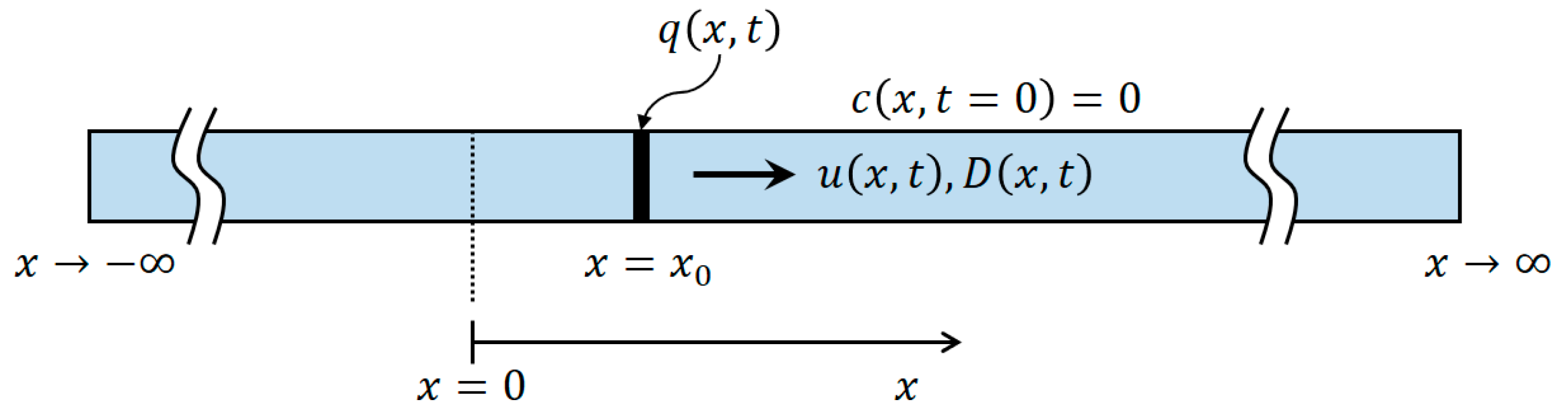
2. Mathematical Formulation and Analytical Solution
2.1. Instantaneous Point Injection
2.2. Continuous Point Injection
2.3. Specific Cases of Dispersion Coefficient and Velocity
2.3.1. Case 1: Spatiotemporally Dependent Dispersion Coefficients and Spatially Dependent Velocities
- (i)
- and .
- (ii)
- and .
- (iii)
- and .
- (iv)
- and .
2.3.2. Case 2: Both Dispersion Coefficient and Velocity Spatially Dependent
2.3.3. Case 3: Spatially Dependent Dispersion Coefficient with Spatiotemporally Dependent Velocity
- (i)
- . Using Equations (10) and (11), we obtain and .
- (ii)
- , and thus and .
- (iii)
- ; therefore, and .
2.3.4. Case 4: Both Dispersion Coefficient and Velocity Spatiotemporally Dependent
- (i)
- , and thus .
- (ii)
- , and thus .
- (iii)
- , and thus .
- (iv)
- , and thus .
3. Verification and Discussion
4. Conclusions
Author Contributions
Funding
Data Availability Statement
Acknowledgments
Conflicts of Interest
Appendix A
Appendix B
References
- Shi, X.; Lei, T.; Yan, Y.; Zhang, F. Determination and impact factor analysis of hydrodynamic dispersion coefficient within a gravel layer using an electrolyte tracer method. Int. Soil Water Conserv. Res. 2016, 4, 87–92. [Google Scholar] [CrossRef] [Green Version]
- Pérez Guerrero, J.S.; Pontedeiro, E.M.; van Genuchten, M.T.; Skaggs, T.H. Analytical solutions of the one-dimensional advection–dispersion solute transport equation subject to time-dependent boundary conditions. Chem. Eng. J. 2013, 221, 487–491. [Google Scholar] [CrossRef]
- Chen, J.-S.; Lai, K.-H.; Liu, C.-W.; Ni, C.-F. A novel method for analytically solving multi-species advective–dispersive transport equations sequentially coupled with first-order decay reactions. J. Hydrol. 2012, 420–421, 191–204. [Google Scholar] [CrossRef]
- Clement, T.P. Generalized solution to multispecies transport equations coupled with a first-order reaction network. Water Resour. Res. 2001, 37, 157–163. [Google Scholar] [CrossRef]
- Clement, T.P.; Srinivasan, V. Analytical solutions for sequentially coupled one-dimensional reactive transport problems—Part I: Mathematical derivations. Adv. Water Resour. 2008, 31, 203–218. [Google Scholar] [CrossRef]
- Corniello, A.; Ducci, D.; Sellerino, M. The hydrogeological monitoring of an experimental site in Campania focused at the evaluation of the contaminants transfer from the soil. Rend. Online Soc. Geol. Ital. 2019, 47, 24–30. [Google Scholar] [CrossRef]
- Kihm, J.-H.; Hwang, G. Numerical simulation of water table drawdown due to groundwater pumping in a contaminated aquifer system at a shooting test site, Pocheon, Korea. Econ. Environ. Geol. 2021, 54, 247–257. [Google Scholar] [CrossRef]
- De Josselin de Jong, G. Longitudinal and transverse diffusion in granular deposits. Trans. Am. Geophys. Union 1958, 39, 67–74. [Google Scholar] [CrossRef]
- Serrano, S.E. The form of the dispersion equation under recharge and variable velocity, and its analytical solution. Water Resour. Res. 1992, 28, 1801–1808. [Google Scholar] [CrossRef]
- Zoppou, C.; Knight, J.H. Analytical solutions for advection and advection-diffusion equations with spatially variable coefficients. J. Hydraul. Eng. 1997, 123, 144–148. [Google Scholar] [CrossRef]
- Singh, M.K.; Singh, V.P.; Singh, P.; Shukla, D. Analytical solution for conservative solute transport in one-dimensional homogeneous porous formations with time-dependent velocity. J. Eng. Mech. 2009, 135, 1015–1021. [Google Scholar] [CrossRef]
- Zamani, K.; Bombardelli, F.A. Analytical solutions of nonlinear and variable-parameter transport equations for verifications of numerical solvers. Environ. Fluid Mech. 2014, 14, 711–742. [Google Scholar] [CrossRef]
- Kinzelbach, W.; Ackerer, P. Modelisation de la propogation d’ un champ d’ écoulement transitoire. Hydrogeology 1986, 2, 197–206. (In French) [Google Scholar]
- Sposito, G.; Weeks, S.W. Tracer advection by steady groundwater flow in a stratified aquifer. Water Resour. Res. 1998, 34, 1051–1059. [Google Scholar] [CrossRef]
- Su, N.; Sander, G.C.; Liu, F.; Anh, V.; Barry, D.A. Similarity solutions for solute transport in fractal porous media using a time- and scale dependent dispersivity. Appl. Math. Model. 2005, 29, 852–870. [Google Scholar] [CrossRef] [Green Version]
- Pang, L.; Hunt, B. Solutions and verification of a scale-dependent dispersion model. J. Contam. Hydrol. 2001, 53, 21–39. [Google Scholar] [CrossRef]
- Moranda, A.; Cianci, R.; Paladino, O. Analytical solutions of one-dimensional contaminant transport in soils with source production-decay. Soil Syst. 2018, 2, 40. [Google Scholar] [CrossRef] [Green Version]
- Paladino, O.; Moranda, A.; Massabò, M.; Robbins, G.A. Analytical solutions of three-dimensional contaminant transport models with exponential source decay. Groundwater 2017, 56, 96–108. [Google Scholar] [CrossRef]
- Stoppiello, M.G.; Lofrano, G.; Carotenuto, M.; Viccione, G.; Guarnaccia, C.; Cascini, L. A comparative assessment of analytical fate and transport models of organic contaminants in unsaturated soils. Sustainability 2020, 12, 2949. [Google Scholar] [CrossRef] [Green Version]
- Gelhar, L.W.; Welty, C.; Rehfeldt, K.R. A critical review of data on field-scale dispersion in aquifers. Water Resour. Res. 1992, 28, 1955–1974. [Google Scholar] [CrossRef]
- Rehfeldt, K.R.; Gelhar, L.W. Stochastic analysis of dispersion in unsteady flow in heterogeneous aquifers. Water Resour. Res. 1992, 28, 2085–2099. [Google Scholar] [CrossRef]
- Neuman, S.P. Universal scaling of hydraulic conductivities and dispersivities in geologic media. Water Resour. Res. 1990, 26, 1749–1758. [Google Scholar] [CrossRef]
- Dagan, G. Solute transport in heterogeneous porous formations. J. Fluid Mech. 1984, 145, 151–177. [Google Scholar] [CrossRef]
- Dagan, G. Time-dependent macrodispersion for solute transport in anisotropic heterogeneous aquifers. Water Resour. Res. 1988, 24, 1491–1500. [Google Scholar] [CrossRef]
- Aral, M.M.; Liao, B. Analytical solutions for two–dimensional transport equations with time-dependent dispersion coefficients. J. Hydrol. Eng. 1996, 1, 20–32. [Google Scholar] [CrossRef]
- Zoua, S.; Ma, J.; Koussis, A.D. Analytical solutions to non-Fickian subsurface dispersion in uniform groundwater flow. J. Hydrol. 1996, 179, 237–258. [Google Scholar] [CrossRef]
- Sposito, G.; Barry, D.A. On the Dagan model of solute transport in groundwater: Foundational aspects. Water Resour. Res. 1987, 23, 1867–1875. [Google Scholar] [CrossRef]
- Basha, H.A.; El-Habel, F.S. Analytical solution of the one-dimensional time dependent transport equation. Water Resour. Res. 1993, 29, 3209–3214. [Google Scholar] [CrossRef]
- Selvadurai, A.P.S. On the advective-diffusive transport in porous media in the presence of time-dependent velocities. Geo. Res. Lett. 2004, 31, 1–5. [Google Scholar] [CrossRef] [Green Version]
- Huang, C.-S.; Tong, C.; Hu, W.-S.; Yeh, H.-D.; Yang, T. Analysis of radially convergent tracer test in a two-zone confined aquifer with vertical dispersion effect: Asymmetrical and symmetrical transports. J. Hazard. Mater. 2019, 377, 8–16. [Google Scholar] [CrossRef] [PubMed]
- Suk, H. Semi-analytical solution of land-derived solute transport under tidal fluctuation in a confined aquifer. J. Hydrol. 2017, 554, 517–531. [Google Scholar] [CrossRef]
- Sternberg, S.P.K.; Cushman, J.H.; Greenkorn, R.A. Laboratory observation of nonlocal dispersion. Trans. Porous Media 1996, 13, 123–151. [Google Scholar] [CrossRef]
- Zhou, R.; Zhan, H.; Chen, K.; Peng, X. Transport in a fully coupled asymmetric stratified system: Comparison of scale dependent and independent dispersion schemes. J. Hydrol. X 2018, 1, 100001. [Google Scholar] [CrossRef]
- Kumar, A.; Jaiswal, D.K.; Kumar, N. Analytical solutions to one-dimensional advection-diffusion equation with variable coefficients in semi-infinite media. J. Hydrol. 2010, 380, 330–337. [Google Scholar] [CrossRef]
- Sanskrityayn, A.; Suk, H.; Kumar, N. Analytical solutions for solute transport in groundwater and riverine flow using Green’s function method and pertinent coordinate transformation method. J. Hydrol. 2017, 547, 517–533. [Google Scholar] [CrossRef]
- Sanskrityayn, A.; Kumar, V.; Kumar, N. Solute transport due to spatio-temporally dependent dispersion coefficient and velocity: Analytical solutions. J. Hydrol. Eng. 2018, 23, 04018009. [Google Scholar] [CrossRef]
- You, K.; Zhan, H. New solutions for solute transport in a finite column with distance-dependent dispersivities and time-dependent solute sources. J. Hydrol. 2013, 487, 87–97. [Google Scholar] [CrossRef]
- Van Genuchten, M.T.; Alves, W.J. Analytical Solutions of the One-Dimensional Convective Dispersive Solute Transport Equations; Technical Bulletin No. 1661; U.S. Department of Agriculture: Washington, DC, USA, 1982.
- Javandel, I.; Doughty, C.; Tsang, C.F. Groundwater Transport Hand Book of Mathematical Models. In AGU Water Resources Monograph Series 10; AGU: Washington, DC, USA, 1984. [Google Scholar]
- Pickens, J.F.; Grisak, G.E. Scale-dependent dispersion in stratified granular aquifer. Water Resour. Res. 1981, 17, 1191–1211. [Google Scholar] [CrossRef]
- Yates, S.R. An Analytical solution for one-dimensional transport in heterogeneous porous media. Water Resour. Res. 1990, 26, 2331–2338. [Google Scholar] [CrossRef]
- Gao, G.; Zhan, H.; Feng, S.; Fu, B.; Ma, Y.; Huang, G. A new mobile-immobile model for reactive solute transport with scale-dependent dispersion. Water Resour. Res. 2010, 46, W08533. [Google Scholar] [CrossRef]
- Hunt, B. Contaminant source solutions with scale-dependent dispersivities. J. Hydrol. Eng. 1998, 3, 268–275. [Google Scholar] [CrossRef]
- Chen, J.S.; Ni, C.F.; Liang, C.P. Analytical power series solution to the two-dimensional advection-dispersion equation with distance-dependent dispersivites. Hydrol. Process. 2008, 22, 4670–4678. [Google Scholar] [CrossRef]
- Chen, J.S.; Ni, C.F.; Liang, C.P.; Chiang, C.C. Analytical power series solution for contaminant transport with hyperbolic asymptotic distance-dependent dispersivity. J. Hydrol. 2008, 362, 142–149. [Google Scholar] [CrossRef]
- Zamani, K.; Bombardelli, F.A. One-dimensional, mass conservative, spatially-dependent transport equation: New analytical solution. In Proceedings of the 12th Pan-American Congress of Applied Mechanics, Port of Spain, Trinidad, 2–6 January 2012. [Google Scholar]
- Kumar, A.; Jaiswal, D.K.; Kumar, N. Analytical solutions of one dimensional advection diffusion equation with variable coefficients in a finite domain. J. Earth Syst. Sci. 2009, 118, 539–549. [Google Scholar] [CrossRef] [Green Version]
- Sanskrityayn, A.; Kumar, N. Analytical solution of advection-diffusion equation in heterogeneous infinite medium using Green’s function method. J. Earth Syst. Sci. 2016, 125, 1713–1723. [Google Scholar] [CrossRef]
- Suk, H. Developing semianalytical solutions for multispecies transport coupled with a sequential first-order reaction network under variable flow velocities and dispersion coefficients. Water Resour. Res. 2013, 49, 3044–3048. [Google Scholar] [CrossRef]
- Suk, H. Generalized semi-analytical solutions to multispecies transport equation coupled with sequential first-order reaction network with spatially or temporally variable transport and decay coefficients. Adv. Water Resour. 2016, 94, 412–423. [Google Scholar] [CrossRef]
- Yeh, G.T. AT123D: Analytical Transient One-, Two-, and Three-Dimensional Simulation of Waste Transport in the Aquifer System; Environmental Sciences Division 1439 Report ORNL-5602; Oak Ridge Natl Lab: Oak Ridge, TN, USA, 1981.
- De Marsily, G. Quantitative Hydrogeology: Groundwater Hydrology for Engineers; Academic Press, Inc.: San Diego, CA, USA, 1986. [Google Scholar]
- Matheron, G.; De Marsily, G. Is transport in porous media always diffusive? A counterexample. Water Resour. Res. 1980, 16, 901–917. [Google Scholar] [CrossRef]
- Haberman, R. Elementry Applied Partial Differential Equations; Prentice-Hall: Englewood Cliffs, NJ, USA, 1987. [Google Scholar]
- Beck, J.V.; Cole, K.D.; Litkouhi, B. Heat Conduction Using Green’s Functions; Hemisphere Publishing Corporation: Washington, DC, USA, 1992. [Google Scholar]
- Yeh, H.D.; Yeh, G.T. Analysis of point-source and boundary-source solutions of one-dimensional groundwater transport equation. J. Environ. Eng. 2007, 133, 1032–1041. [Google Scholar] [CrossRef] [Green Version]
- Yeh, G.T.; Cheng, J.R. 2DFATMIC: User’s Manual of a Two-Dimensional Subsurface Flow, Fate and Transport of Microbes and Chemical Model Version 1.0. EPA/600/R-97/052; U.S. Environmental Protection Agency: Washington, DC, USA, 1997.


| Sect. | Dispersion Coefficient, D | Velocity, u | Source | Ref. | |||||||
|---|---|---|---|---|---|---|---|---|---|---|---|
| a C | b L | c T | d S | a C | b L | c T | d S | § I | † C | ||
| 2.3.1 | ● | ● | ● | Not existed | |||||||
| ● | ● | ● | Not existed | ||||||||
| ● | ● | ● | [28] | ||||||||
| ● | ● | ● | [28] | ||||||||
| 2.3.2 | ● | ● | ● | [36] | |||||||
| ● | ● | ● | [36] | ||||||||
| ● | ● | ● | [51] | ||||||||
| ● | ● | ● | [52] | ||||||||
| 2.3.3 | ● | ● | ● | Not existed | |||||||
| ● | ● | ● | Not existed | ||||||||
| ● | ● | ● | [29] | ||||||||
| ● | ● | ● | [29] | ||||||||
| 2.3.4 | ● | ● | ● | [36] | |||||||
| ● | ● | ● | [36] | ||||||||
| ● | ● | ● | [36] | ||||||||
| ● | ● | ● | [11,36] | ||||||||
| Figs | u0 (m/Day) | D0 (m2/Day) | x0 (m) | t (day) | a (m−1) | b (-) | m (Day−1), k (Day) | M (g/m2), C0 (g/m3) |
|---|---|---|---|---|---|---|---|---|
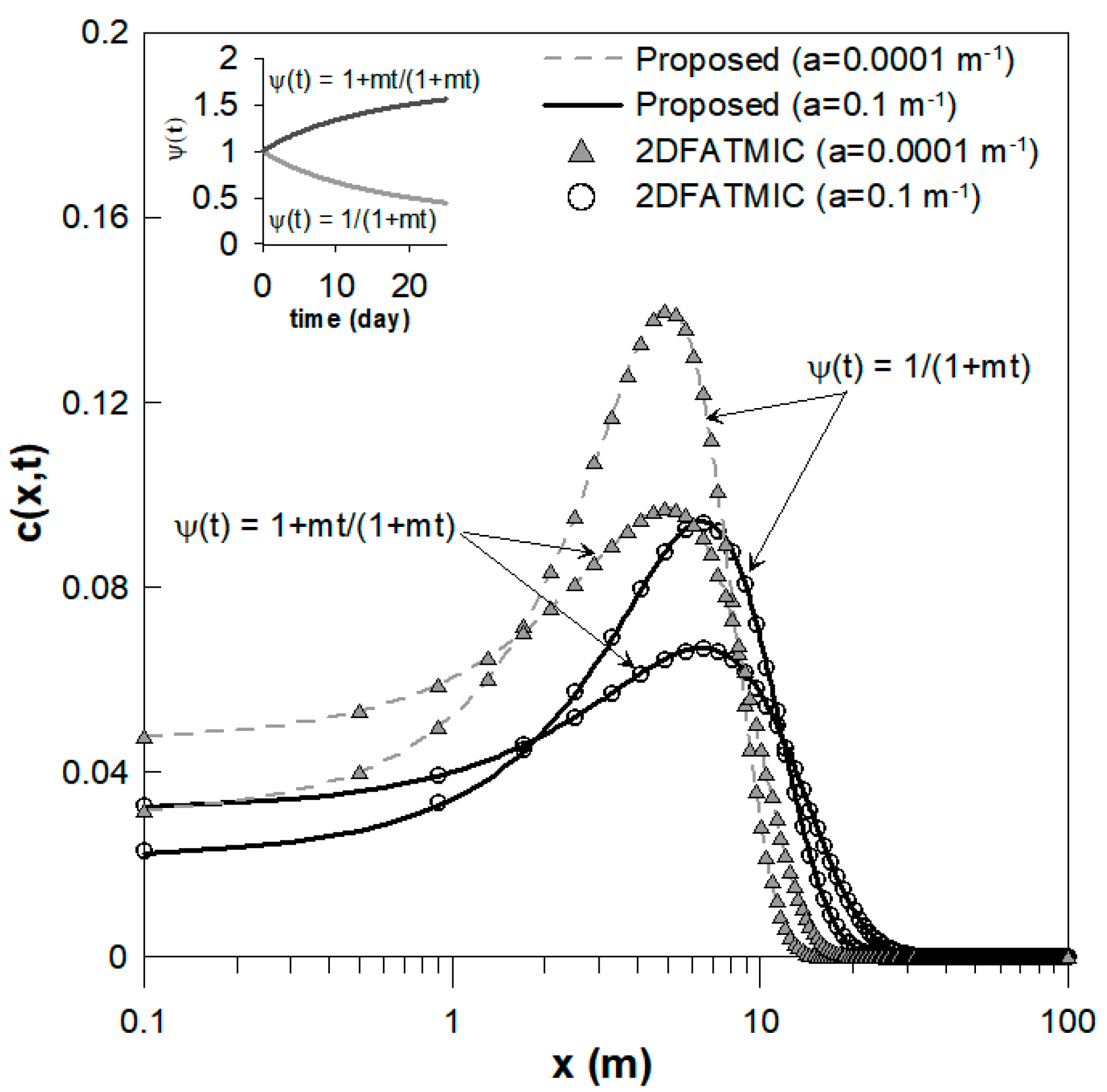
| Figure 2 | D(x,t) = D0(1 + ax)ψ(t) and u(x) = u0(1 + ax) | |||||||
| 0.20 | 0.25 | 0 | 25 | 0.1, 0.0001 | 1 | m = 0.05 | M = 1 | |
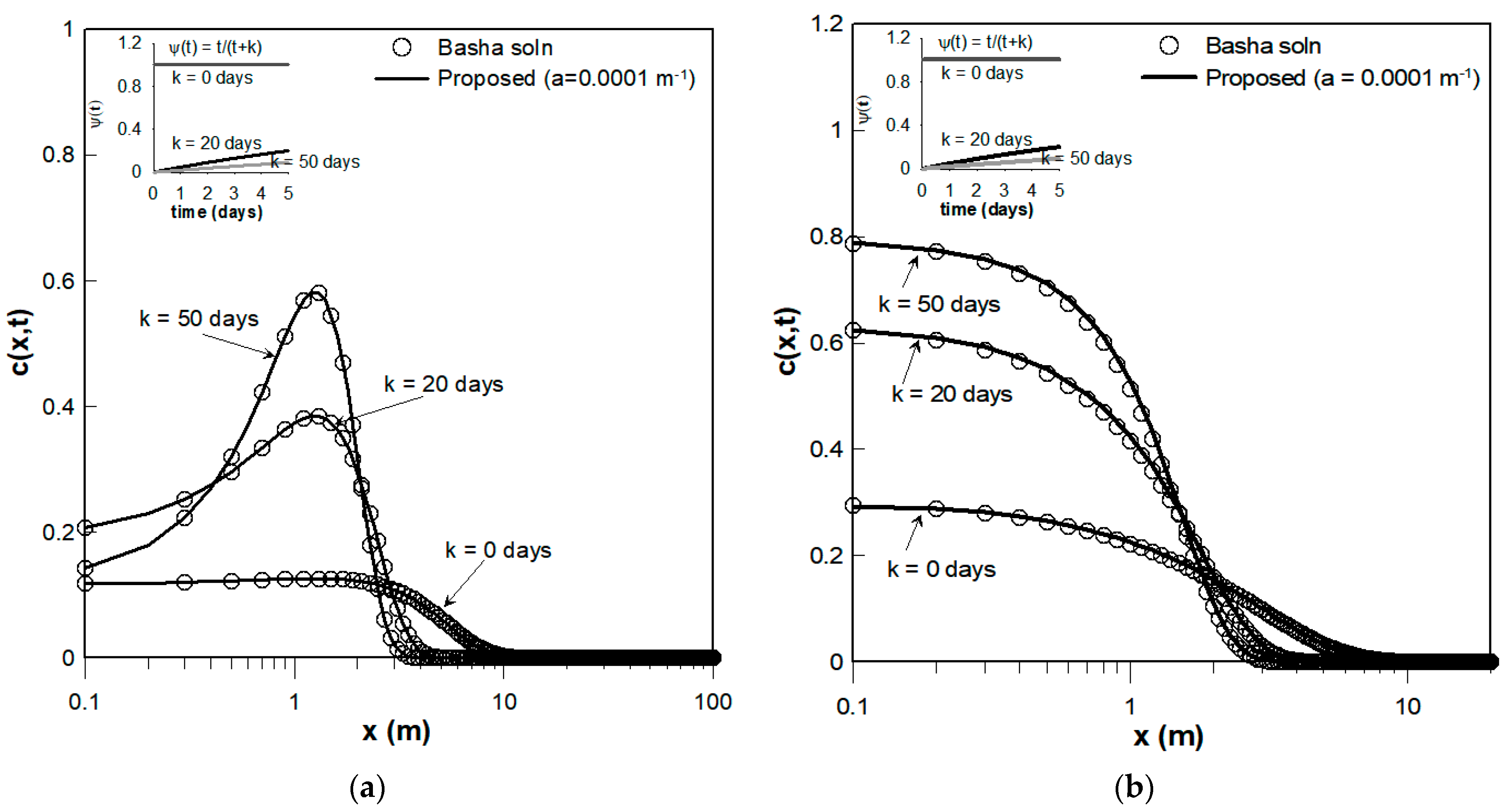
| D(t) = D0ψ(t) and u = u0 | ||||||||
| Figure 3a | 0.25 | 1.0 | 0 | 5 | 0.1, 0.0001 | 1 | k = 0,20,50 | M = 1 |
| Figure 3b | 0.25 | 1.0 | 0 | 5 | 0.1, 0.0001 | 1 | k = 0,20,50 | C0 = 1 |
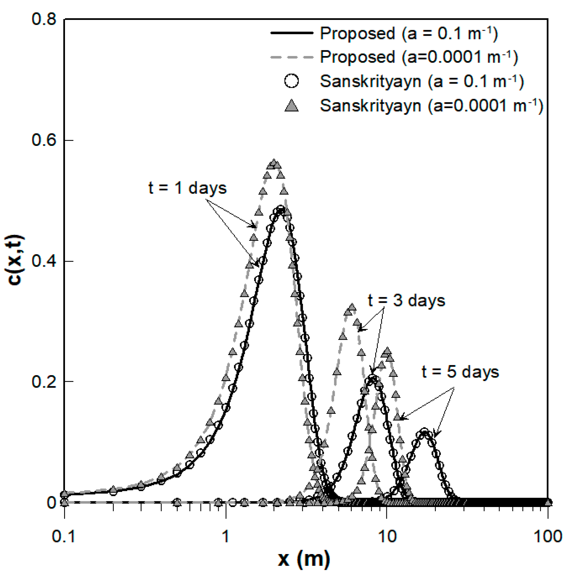
| Figure 4 | D(x) = D0(1 + ax) and u(x) = u0(1 + ax) | |||||||
| 2.0 | 0.25 | 0 | 1, 3, 5 | 0.1, 0.0001 | 1 | - | M = 1 | |
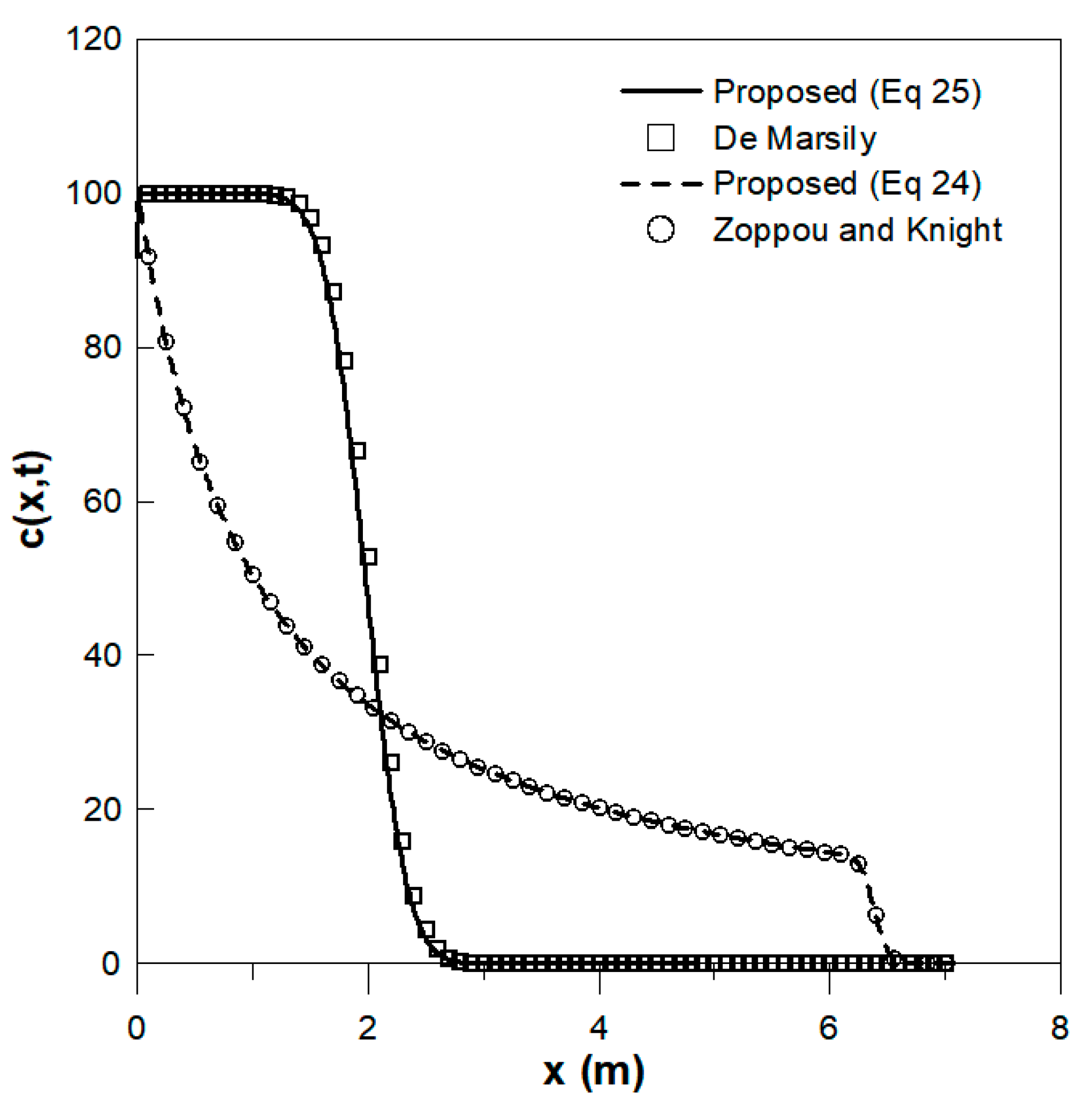
| Figure 5 | D = D0, u = u0 for Equation (25) and D(x) = D0 x, u(x) = u0 x for Equation (24) | |||||||
| Equation (25) 1.0 Equation (24) 1.0 | 0.02 0.0001 | 0 1 | 2 2 | 0 1 | 1 0 | - - | C0 = 100 C0 = 100 | |
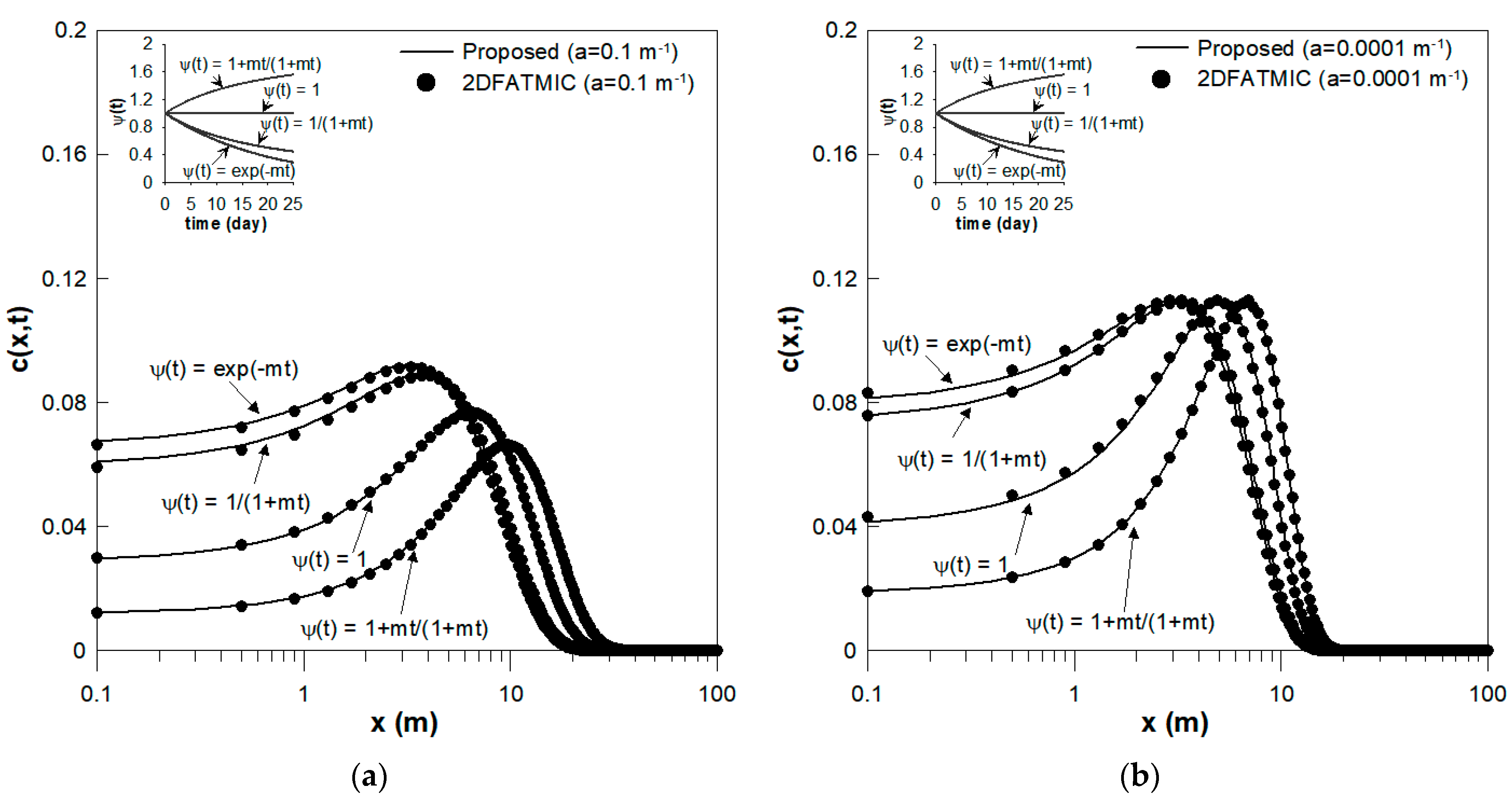
| Figure 6a,b | D(x) = D0(1 + ax) and u(x,t) = u0(1 + ax) ψ(t) | |||||||
| 0.20 | 0.25 | 0 | 25 | 0.1, 0.0001 | 1 | m = 0.05 | M = 1 | |
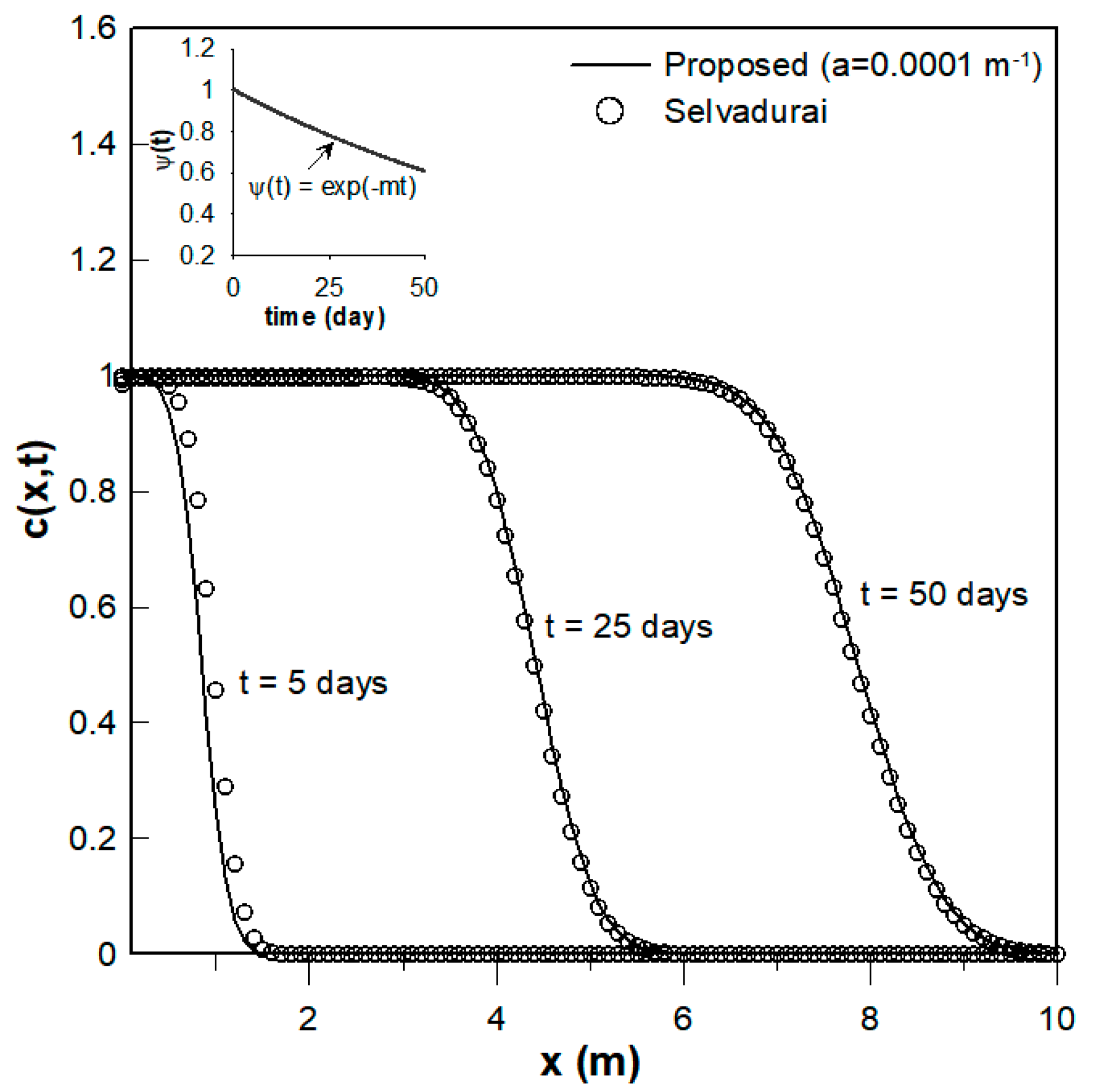
| Figure 7 | D = D0 and u(t) = u0 ψ(t) | |||||||
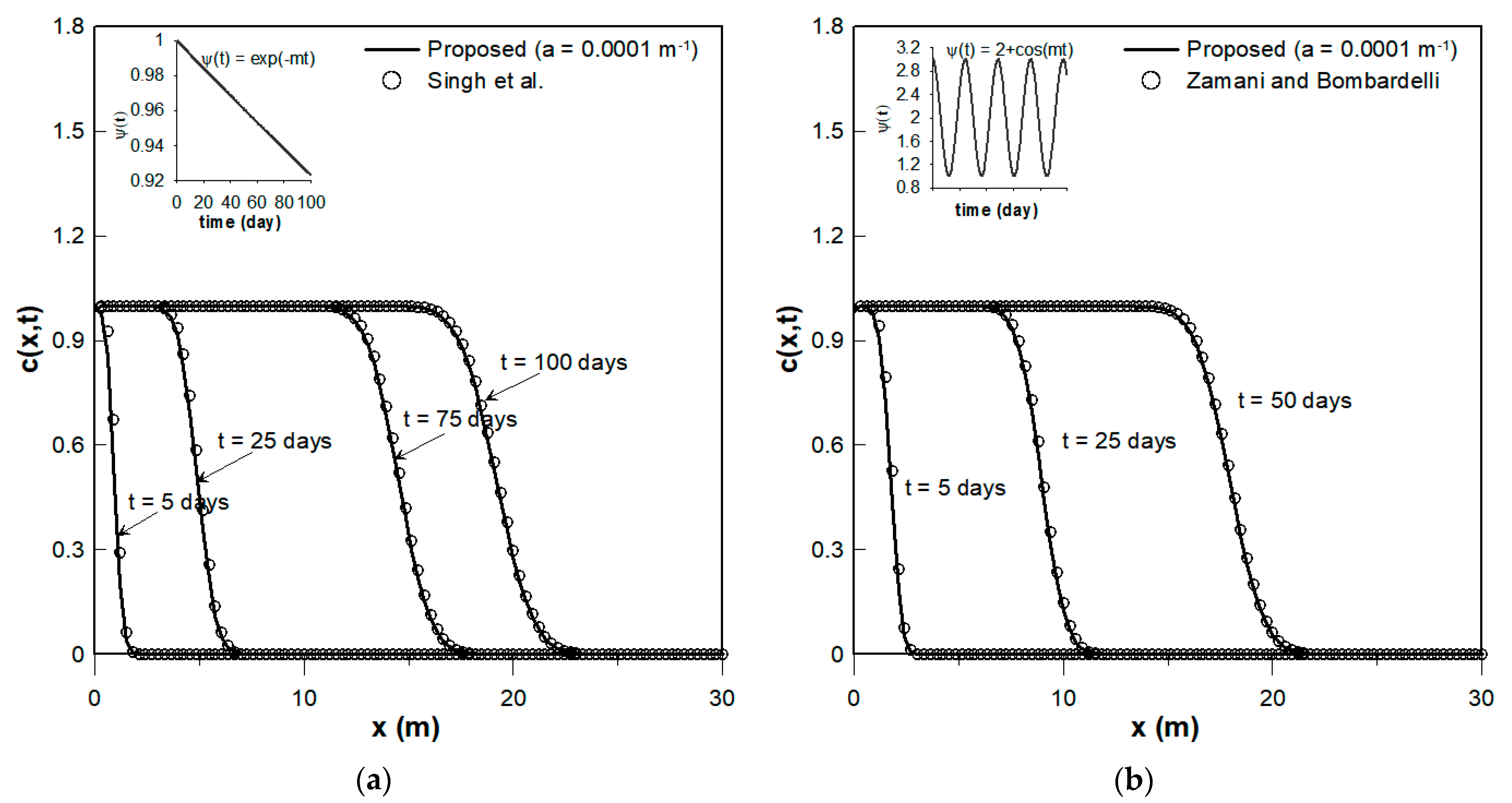
| 0.20 | 0.005 | 0 | 5, 25, 50 | 0.0001 | 1 | m = 0.01 | C0 = 1 | |
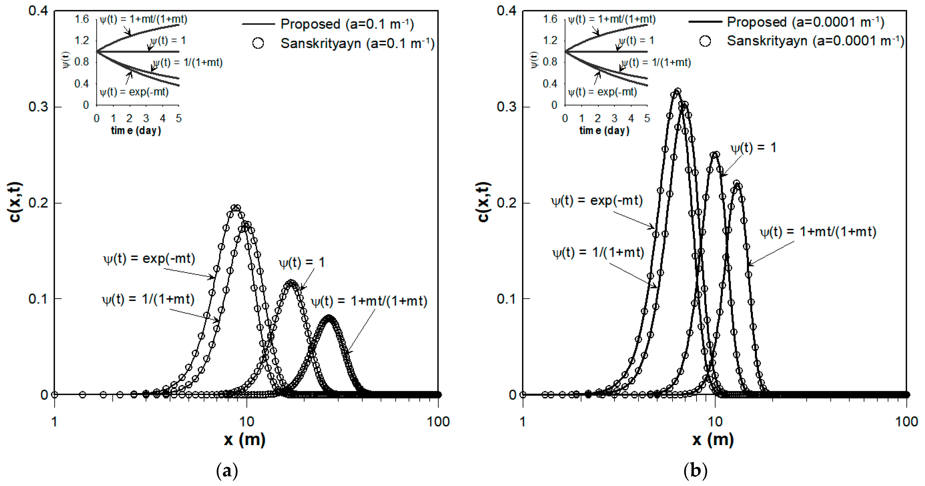
| Figure 8a,b | D(x,t) = D0(1 + ax)ψ(t) and u(x,t) = u0(1 + ax) ψ(t) | |||||||
| 2.0 | 0.25 | 0 | 5 | 0.1, 0.0001 | 1 | m = 0.2 | M = 1 | |
| D(t) = D0 ψ(t) and u(t) = u0 ψ(t) | ||||||||
| Figure 9a | 0.20 | 0.01 | 0 | 5, 25, 50,100 | 0.0001 | 1 | M = 0.0008 | C0 = 1 |
| Figure 9b | 0.20 | 0.01 | 0 | 5, 25, 50 | 0.0001 | - | M = 12.41 | C0 = 1 |
Publisher’s Note: MDPI stays neutral with regard to jurisdictional claims in published maps and institutional affiliations. |
© 2021 by the authors. Licensee MDPI, Basel, Switzerland. This article is an open access article distributed under the terms and conditions of the Creative Commons Attribution (CC BY) license (https://creativecommons.org/licenses/by/4.0/).
Share and Cite
Sanskrityayn, A.; Suk, H.; Chen, J.-S.; Park, E. Generalized Analytical Solutions of The Advection-Dispersion Equation with Variable Flow and Transport Coefficients. Sustainability 2021, 13, 7796. https://0-doi-org.brum.beds.ac.uk/10.3390/su13147796
Sanskrityayn A, Suk H, Chen J-S, Park E. Generalized Analytical Solutions of The Advection-Dispersion Equation with Variable Flow and Transport Coefficients. Sustainability. 2021; 13(14):7796. https://0-doi-org.brum.beds.ac.uk/10.3390/su13147796
Chicago/Turabian StyleSanskrityayn, Abhishek, Heejun Suk, Jui-Sheng Chen, and Eungyu Park. 2021. "Generalized Analytical Solutions of The Advection-Dispersion Equation with Variable Flow and Transport Coefficients" Sustainability 13, no. 14: 7796. https://0-doi-org.brum.beds.ac.uk/10.3390/su13147796