
CO2 Emission and Cost Optimization of Concrete-Filled Steel Tubular (CFST) Columns Using Metaheuristic Algorithms


Abstract
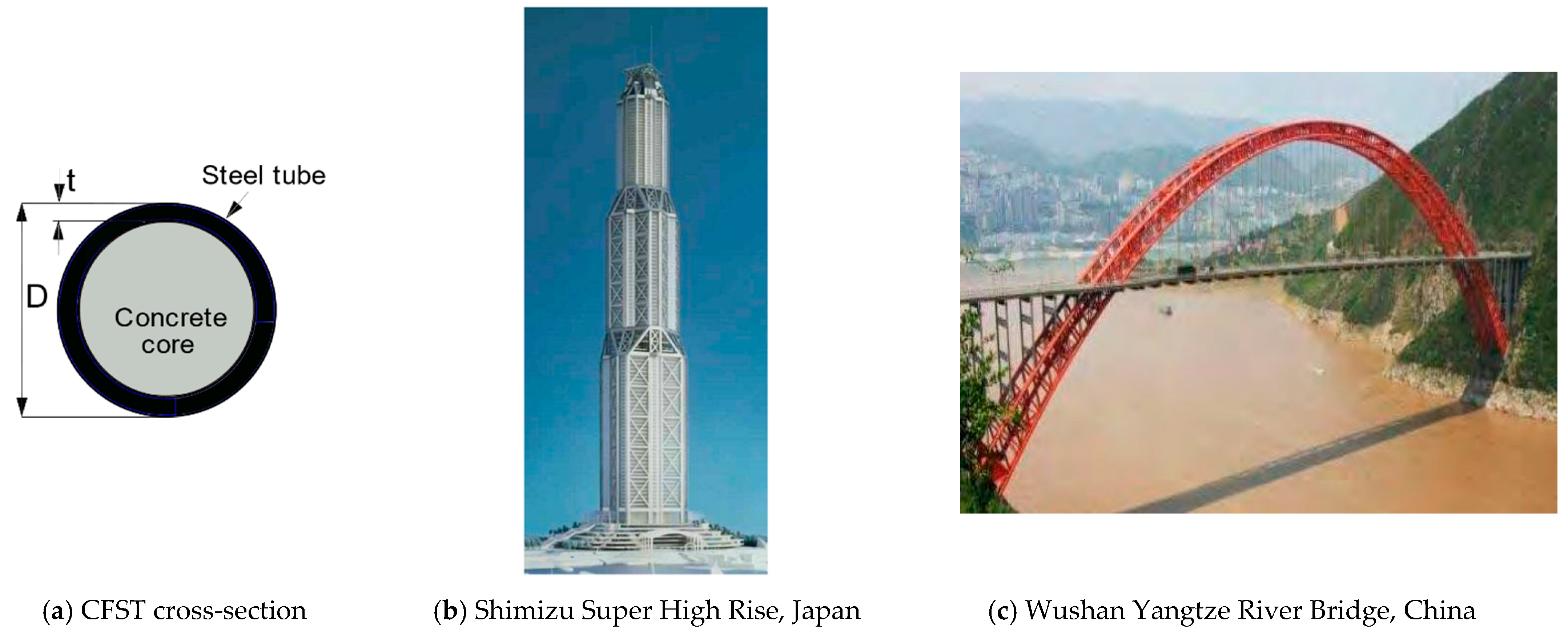
:1. Introduction
2. CO2 Emission and Structural Design
3. Axial Capacity of CFST Columns
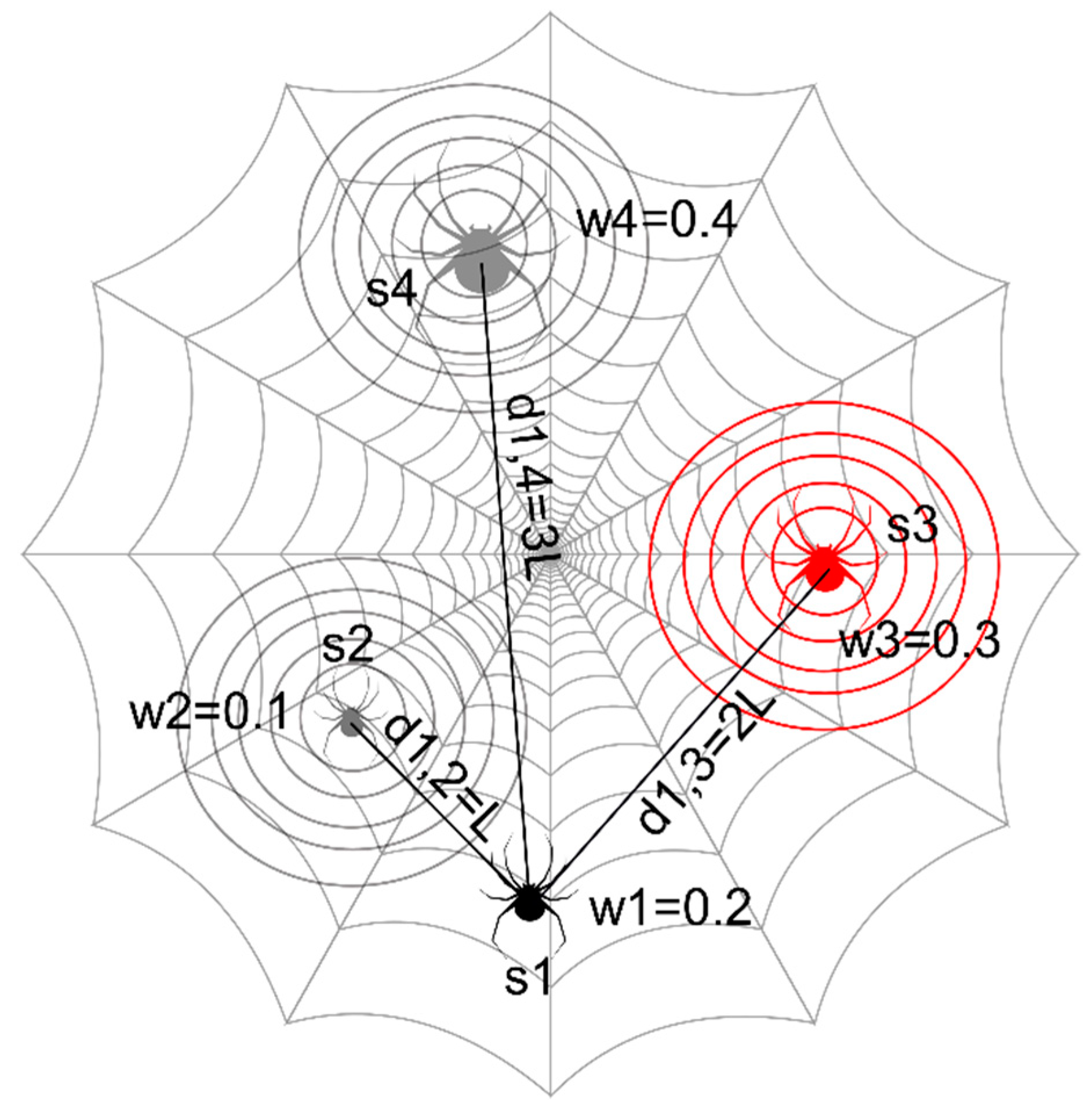
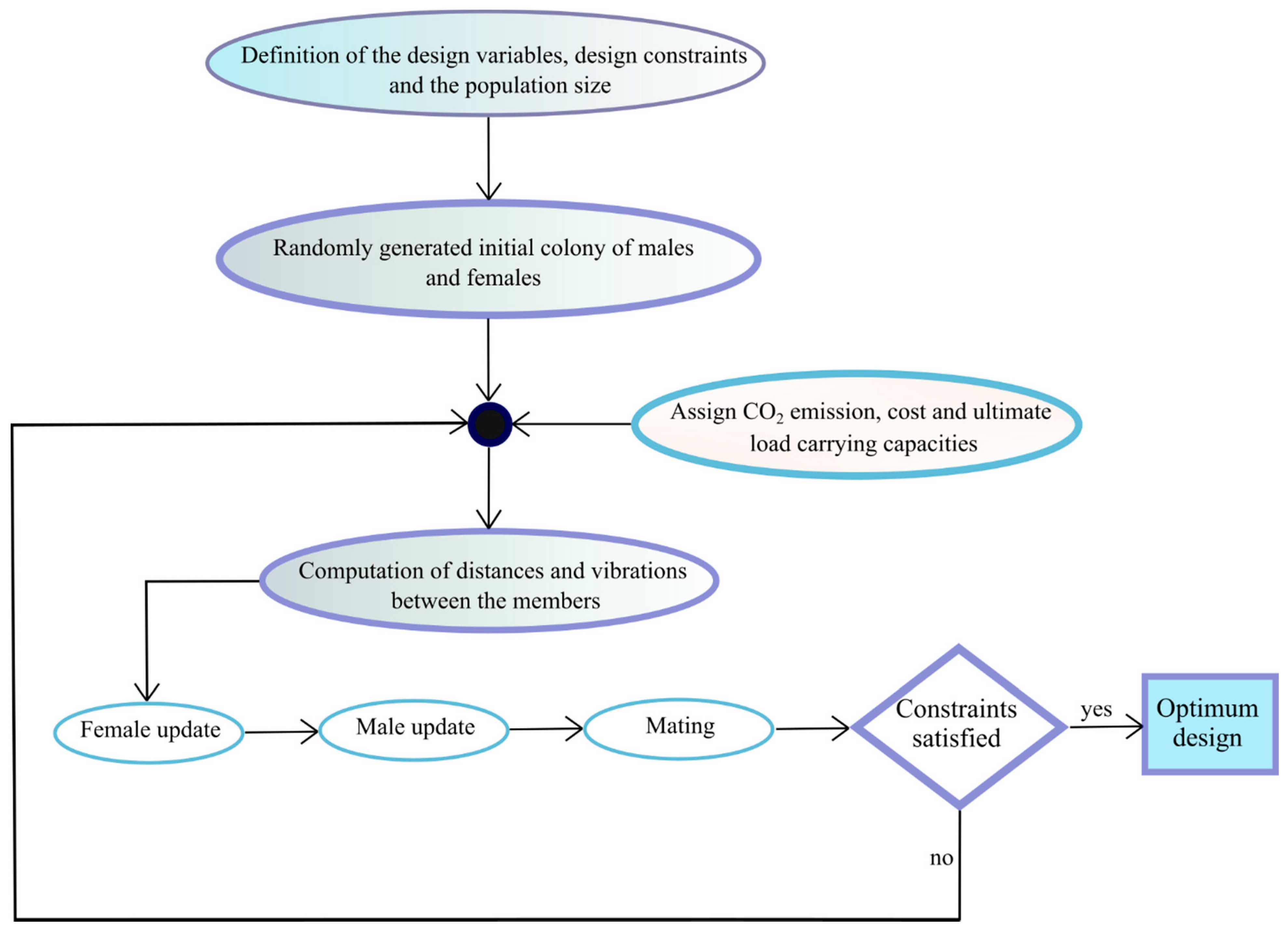
4. Metaheuristic Optimization Methodology
Computational Procedure
| Algorithm 1: Pseudocode for the initialization of the spider colony. |
| Fori = 1 to N (number of colony members) For j = 1 to n (number of design variables) Spiders[i,j] = low + (high—low) (rand) Check if Nu ≥ Nu,min Repeat until Nu ≥ Nu,min |
| Algorithm 2: Connectivity of the spiders. |
| Fori = 1 to N For j = 1 to N Distance matrix[i,j] = Distance(spiders[i], spiders[j]) Scaled distance matrix = Distance matrix/max (Distance matrix) For i = 1 to N For j = 1 to N vibration matrix[i,j] = distance(spiders[i], spiders[j]) |
| Algorithm 3: Iteration of the female spiders. |
| Functionmove females Generate For i = 1 to Nf Find the best performing and the nearest better performing members If 0.7 then apply attraction Else apply repulsion Compute cross-section area and Nu Repeat until Nu ≥ Nu,min |
| Algorithm 4: Iteration of the male spiders. |
| Functionmove males Compute the weighted mean of the males Sort the males and find the median male For i = Nf to N If Spiders[i] is dominant then find the nearest female to Spiders[i] Apply attraction towards the nearest female Else move towards the weighted mean of the male population |
| Algorithm 5: Control of the variable ranges. |
| Functioncontrol variable ranges For i = 1 to N For j = 1 to n If Spiders[i,j] violates the boundaries then Spiders[i] = randomly generated member Compute area and Nu for the new member Repeat until Nu ≥ Nu,min |
| Algorithm 6: Mating. |
| Function Mating For m = Nf + 1 to N If Spiders[m] is a dominant male then Create empty set for mating For f = 1 to Nf If Distance matrix [m,f] ≤ radius of mating Add Spiders[f] to mating set Compute the weight distribution inside the mating set Generate new member with the properties of the best spider in the mating set If weight of the new spider > the weight of the worst spider then Replace the worst spider with the new spider |
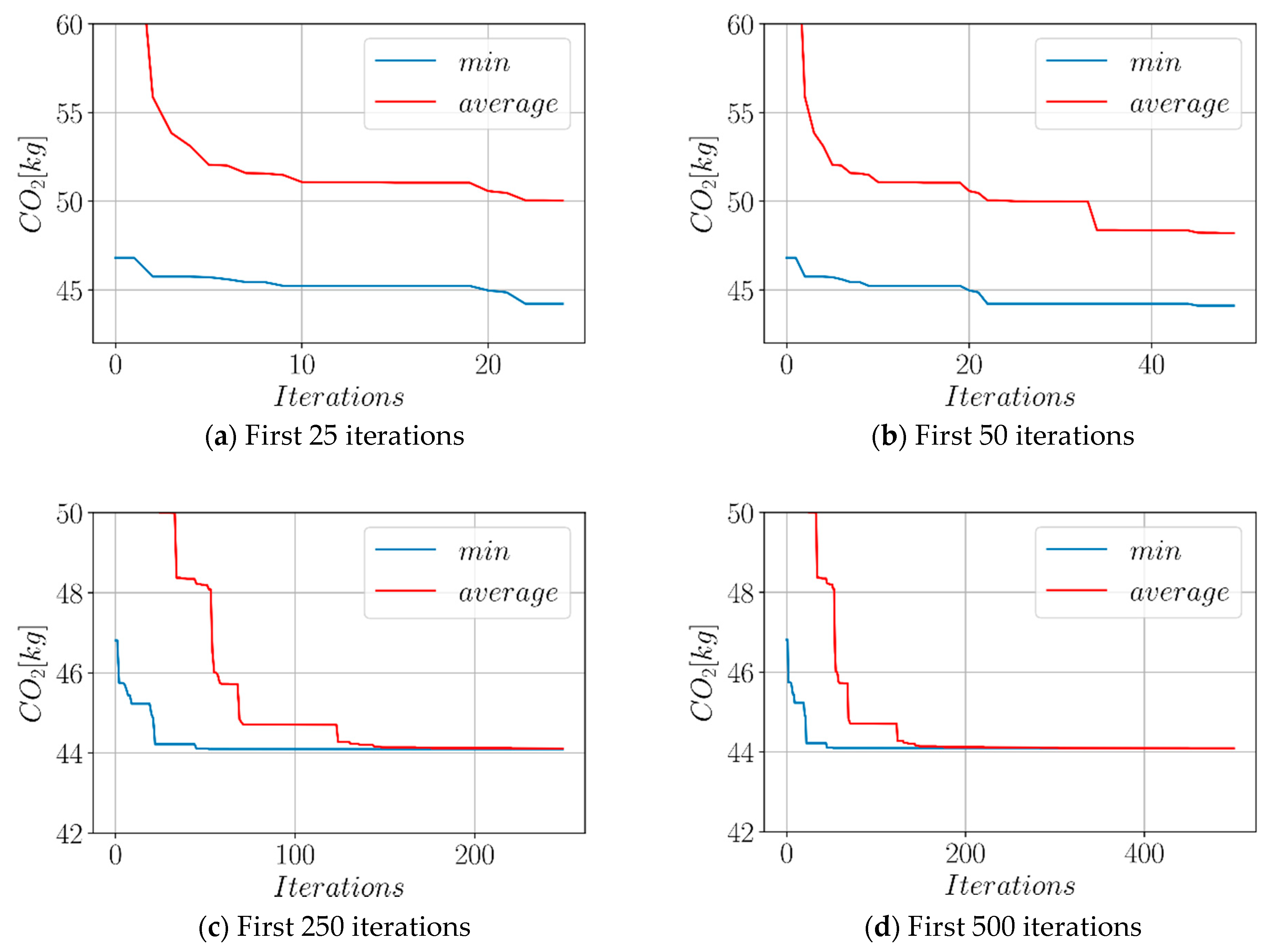
5. Results and Discussions
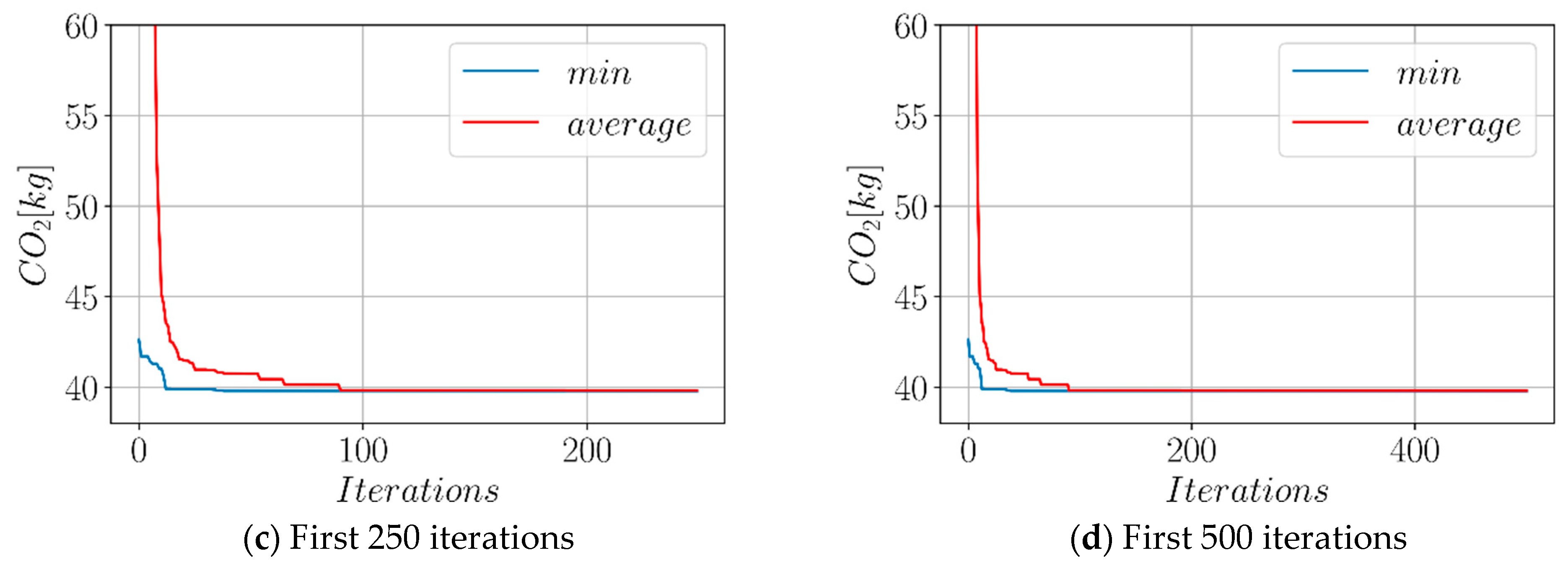
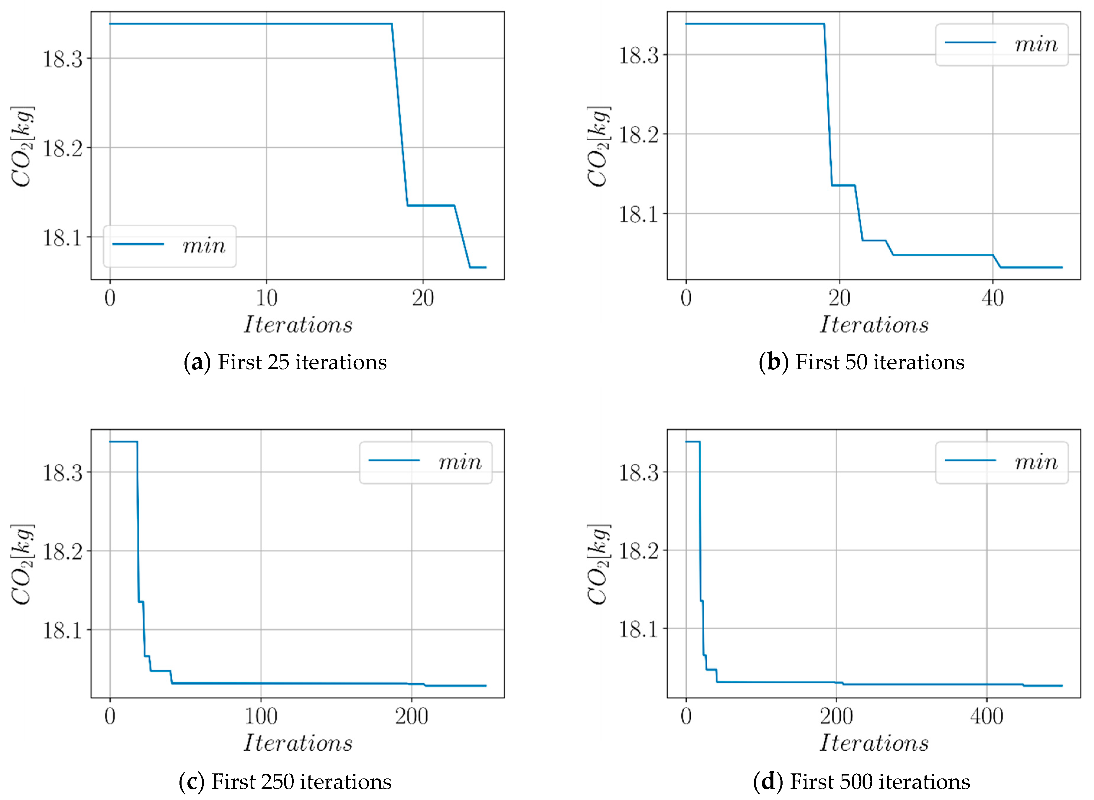
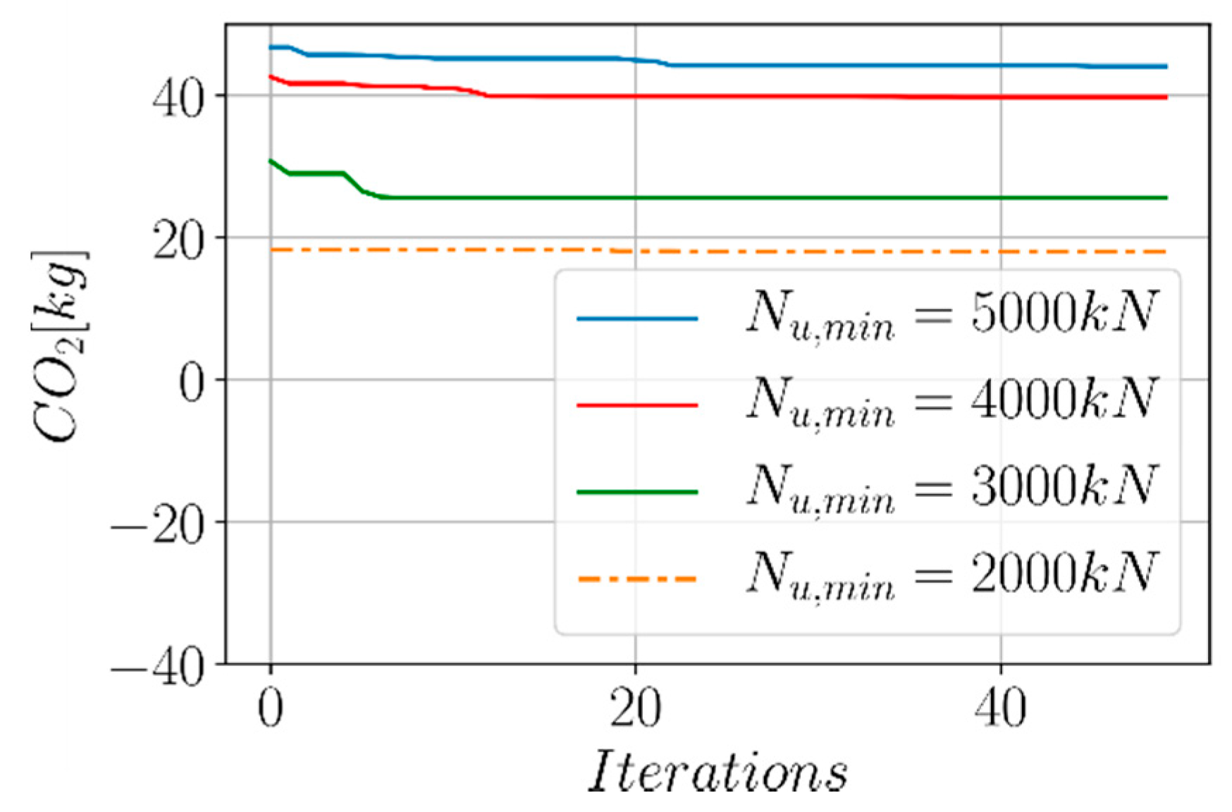
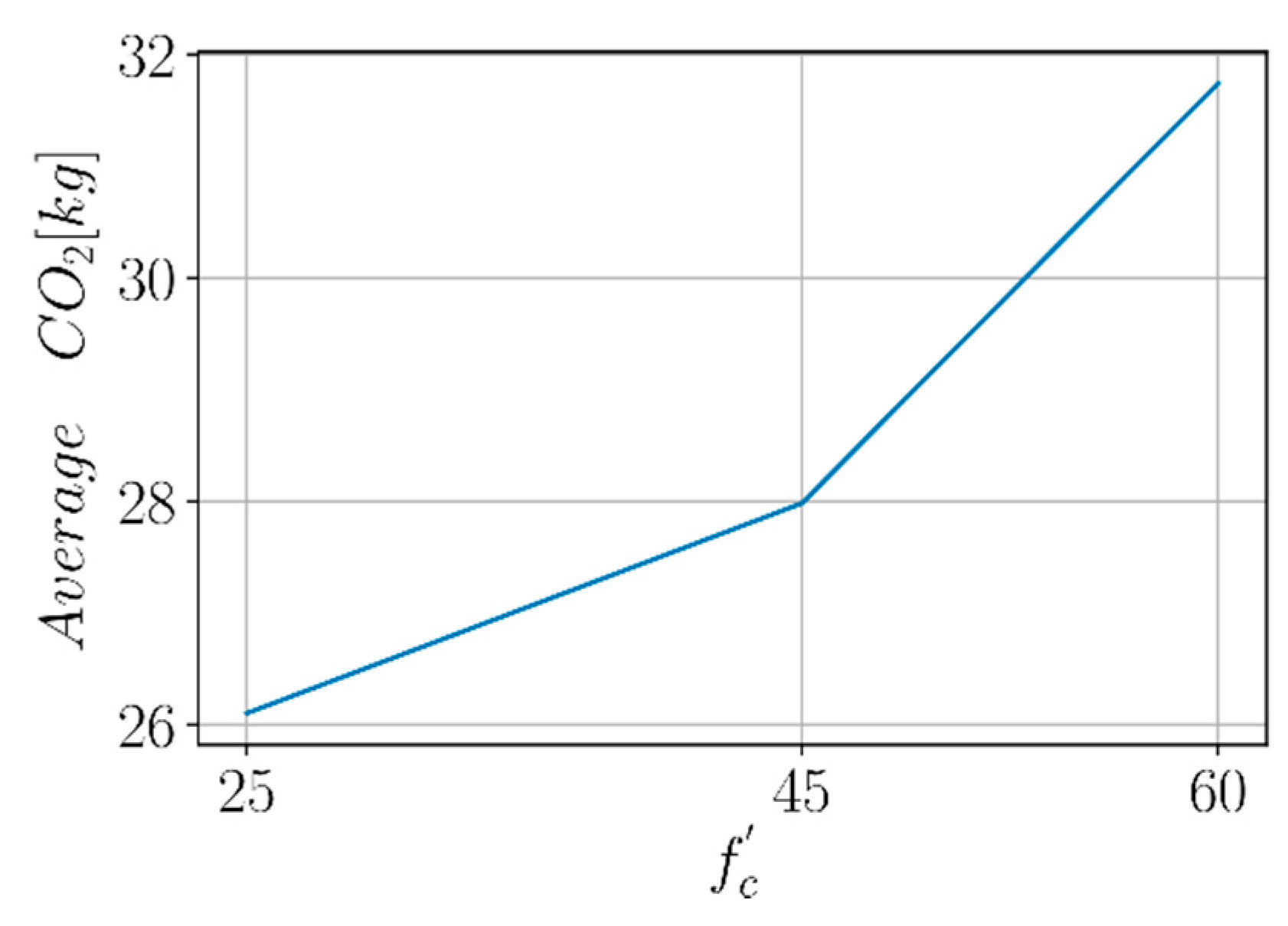
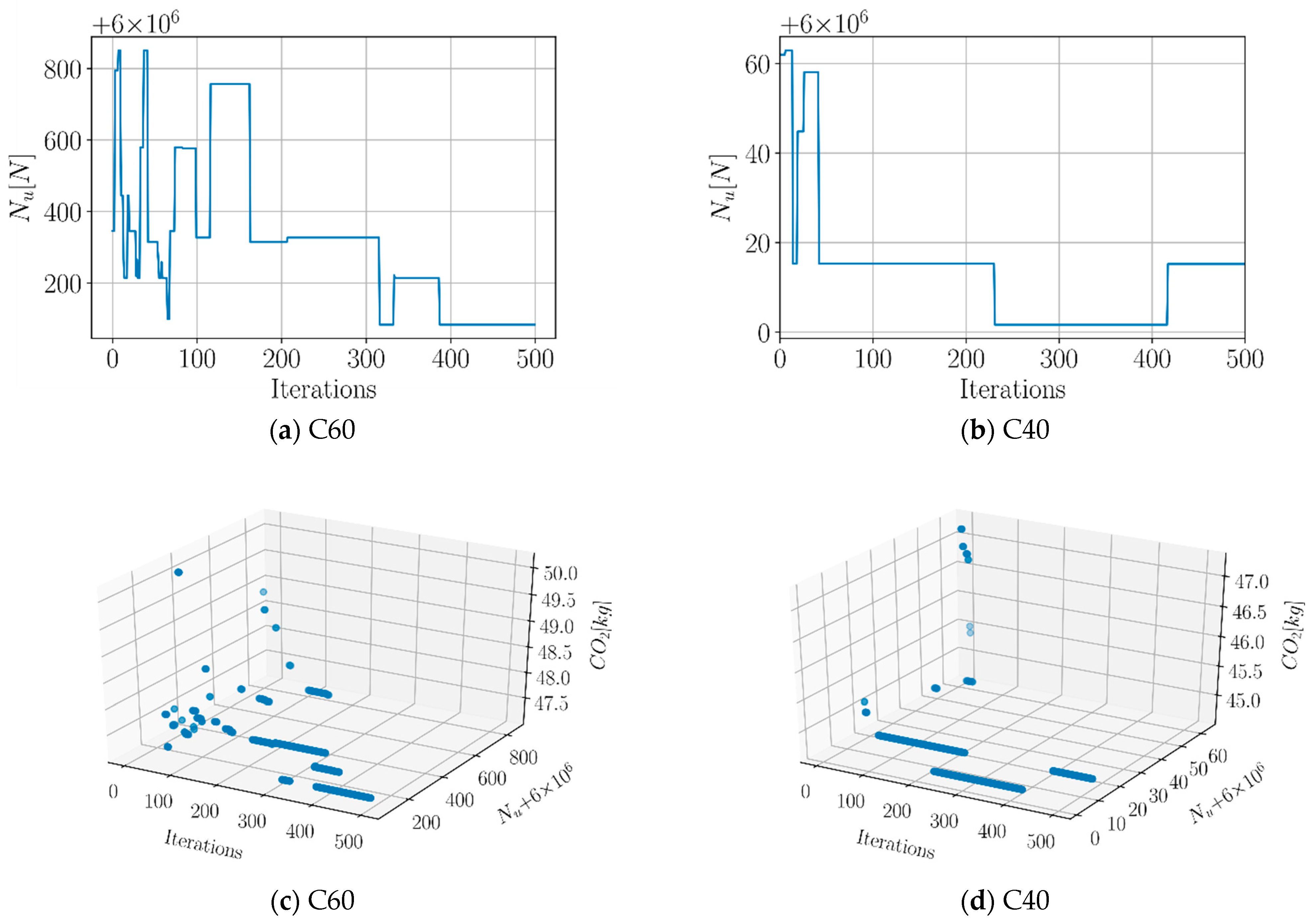
5.1. Optimization of the CO2 Emission
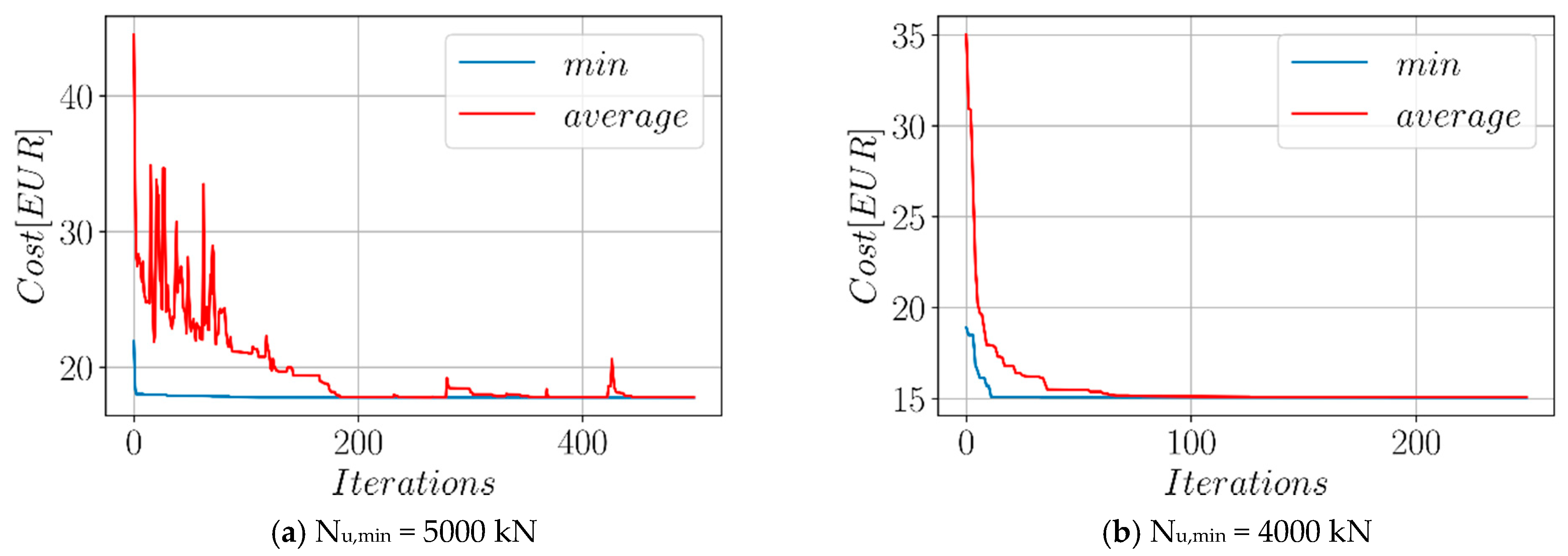
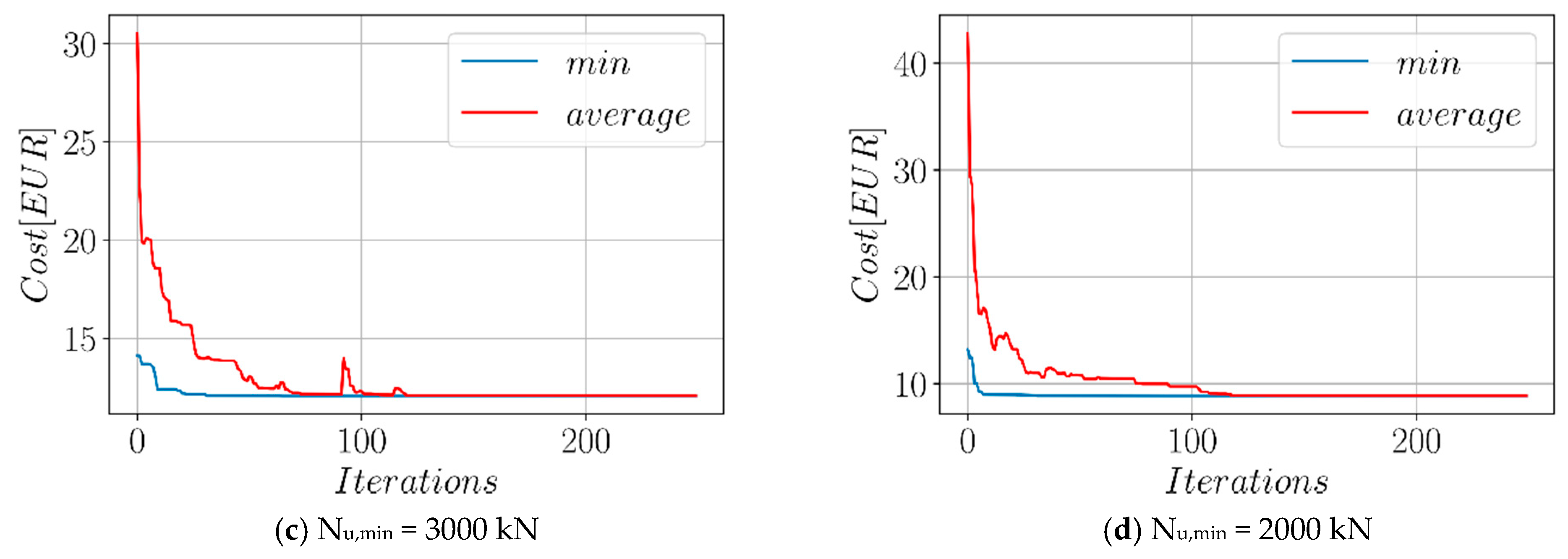
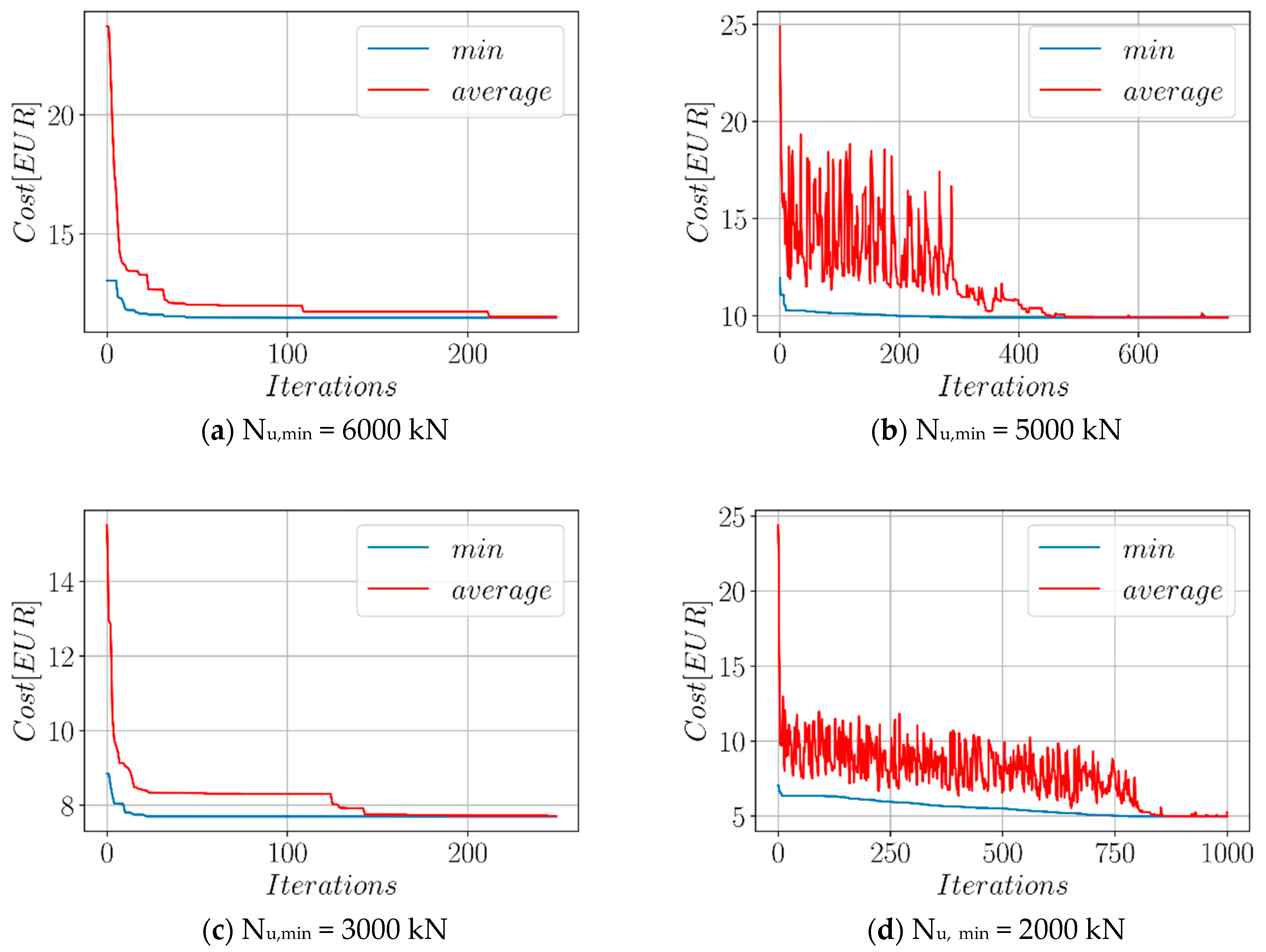
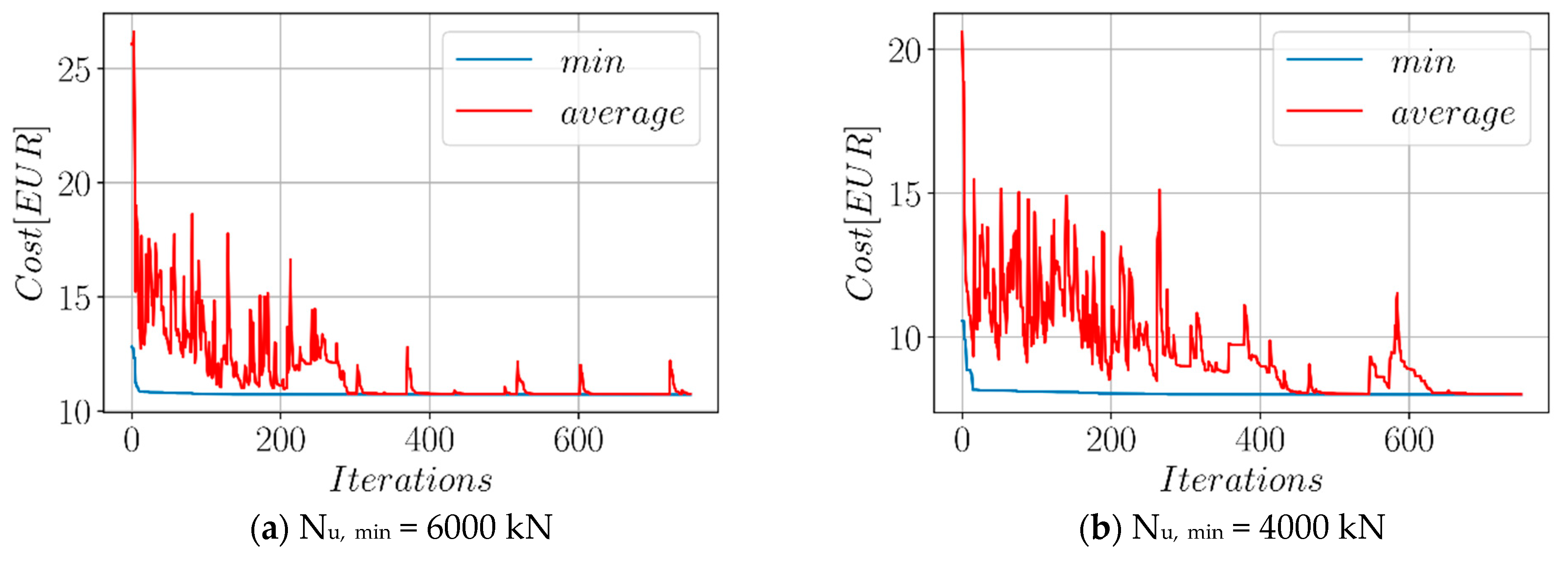
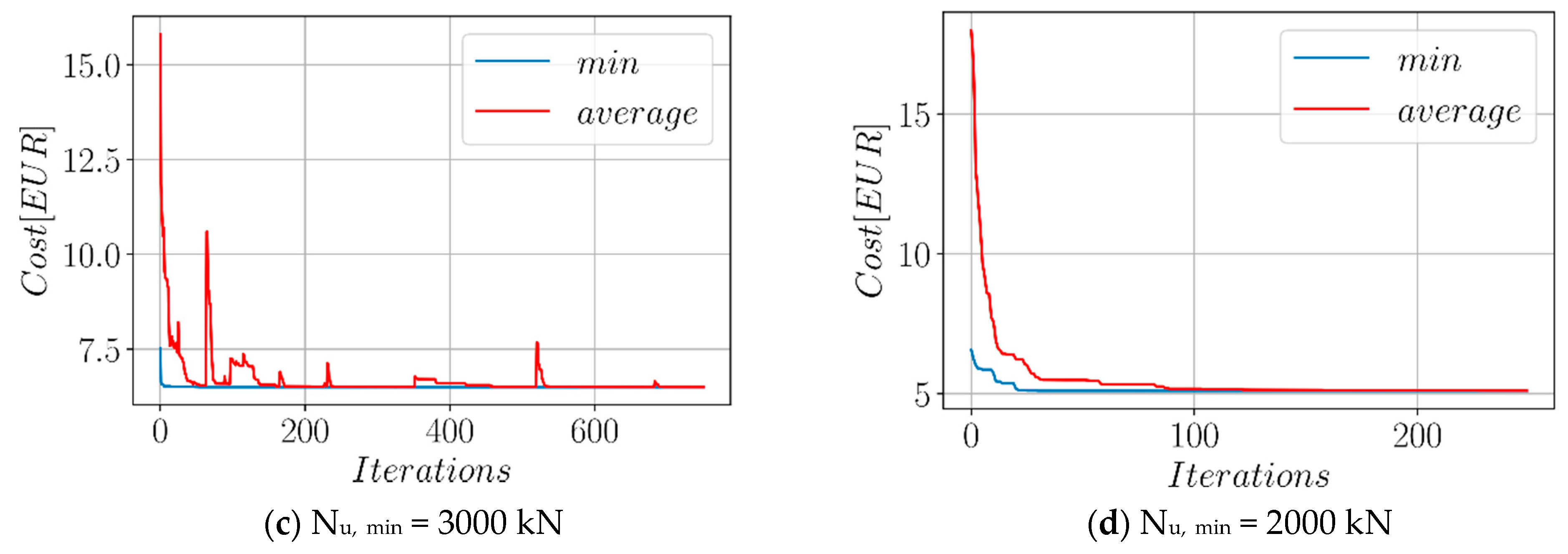
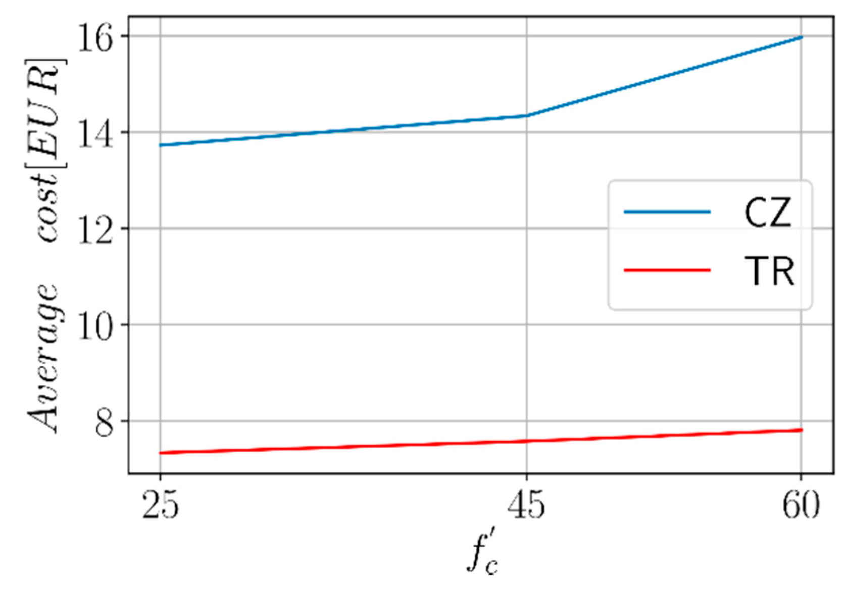
5.2. Optimization of the Cost
6. Conclusions
- The results of the optimization showed that, on average, using concrete with lower compressive strength is favorable in terms of both CO2 emissions and cost.
- In general, having a smaller wall thickness for the steel casing has a favorable effect on both the CO2 emissions and the cost since the optimum wall thickness is near the lower bound for this variable at most load levels.
- In the majority of the investigated cases, a decrease in the outer diameter and the D/t ratio was also associated with a decrease in cost and CO2 emissions.
- Designs that lead to lower carbon emissions also tend to have a lower cost.
Author Contributions
Funding
Conflicts of Interest
References
- Wei, J.; Luo, X.; Lai, Z.; Varma, A.H. Experimental Behavior and Design of High-Strength Circular Concrete-Filled Steel Tube Short Columns. J. Struct. Eng. 2019, 146, 04019184. [Google Scholar] [CrossRef]
- Nguyen, T.T.; Thai, H.T.; Ngo, T.; Uy, B.; Li, D. Behaviour and design of high strength CFST columns with slender sections. J. Constr. Steel Res. 2021, 182, 106645. [Google Scholar] [CrossRef]
- Duong, H.T.; Phan, H.C.; Le, T.T.; Bui, N.D. Optimization design of rectangular concrete-filled steel tube short columns with Balancing Composite Motion Optimization and data-driven model. Structures 2020, 28, 757–765. [Google Scholar] [CrossRef]
- Shieh, S.S.; Chang, C.C.; Jong, J.H. Structural design of composite super-columns for the Taipei 101 Tower. In Proceedings of the International Workshop on Steel and Concrete Composite Constructions, Sydney, Australia, 22–25 June 2003; pp. 25–33. [Google Scholar]
- Han, L. Tests on stub columns of concrete-filled RHS sections. J. Constr. Steel Res. 2002, 58, 353–372. [Google Scholar] [CrossRef]
- Han, L.; Yao, G.; Zhao, X. Tests and calculations for hollow structural steel (HSS) stub columns filled with self-consolidating concrete (SCC). J. Constr. Steel Res. 2005, 61, 1241–1269. [Google Scholar] [CrossRef]
- Schneider, S. Axially Loaded Concrete-Filled Steel Tubes. J. Struct. Eng. 1998, 124, 1125–1138. [Google Scholar] [CrossRef]
- Sakino, K.; Tomii, M.; Watanabe, K. Sustaining load capacity of plain concrete stub columns by circular steel tubes. In Proceedings of the International Speciality Conference on Concrete-Filled Steel Tubular Structure, Harbin, China, 12–15 August 1985; pp. 112–118. [Google Scholar]
- Huang, F.; Yu, X.; Chen, B. The structural performance of axially loaded CFST columns under various loading conditions. Steel Compos. Struct. 2012, 13, 451–471. [Google Scholar] [CrossRef]
- Yang, Y.F.; Ma, G.L. Experimental behaviour of recycled aggregate concrete filled stainless steel tube stub columns and beams. Thin Walled Struct. 2013, 66, 62–75. [Google Scholar] [CrossRef]
- Uenaka, K.; Kitoh, H.; Sonoda, K. Concrete Filled Double Skin Circular Stub Columns Under Compression. Thin-Walled Struct. 2010, 48, 19–24. [Google Scholar] [CrossRef]
- Perea, T.; Leon, R.T.; Hajjar, J.F.; Denavit, M.D. Full-Scale Tests of Slender Concrete-Filled Tubes: Axial Behavior. J. Struct. Eng. 2013, 139, 1249–1262. [Google Scholar] [CrossRef]
- American Institute of Steel Construction (AISC). Specification for Structural Steel Buildings; AISC 360-16; American Institute of Steel Construction: Chicago, IL, USA, 2016. [Google Scholar]
- European Committee for Standardization (CEN). Design of Composite Steel and Concrete Structures—Part 1-1: General Rules and Rules for Buildings; EN 1994-1-1 Eurocode 4; European Committee for Standardization: Brussels, Belgium, 2004. [Google Scholar]
- Canadian Standards Association. Design of Steel Structures—CSA S16, 9th ed.; Canadian Standards Association: Mississauga, ON, Canada, 2019; ISBN 978-1-4883-1548-0. [Google Scholar]
- Standards Australia. AS 5100.1 2017: Bridge Design, Part 1: Scope and General Principles; Standards Australia: Sydney, Australia, 2017. [Google Scholar]
- Liu, D.; Gho, W.M. Axial load behaviour of high-strength rectangular concrete-filled steel tubular stub columns. Thin Walled Struct. 2005, 43, 1131–1142. [Google Scholar] [CrossRef]
- Thai, H.T.; Uy, B.; Khan, M.; Tao, Z.; Mashiri, F. Numerical modelling of concrete-filled steel box columns incorporating high strength materials. J. Constr. Steel Res. 2014, 102, 256–265. [Google Scholar] [CrossRef]
- Khan, M.; Uy, B.; Tao, Z.; Mashiri, F. Concentrically loaded slender square hollow and composite columns incorporating high strength properties. Eng. Struct. 2016, 131, 69–89. [Google Scholar] [CrossRef]
- Khan, M.; Uy, B.; Tao, Z.; Mashiri, F. Behaviour and design of short high-strength steel welded box and concrete-filled tube (CFT) sections. Eng. Struct. 2017, 147, 458–472. [Google Scholar] [CrossRef]
- Saadoon, A.S.; Nasser, K.Z. Mohamed IQ. A neural network model to predict ultimate strength of rectangular concrete filled steel tube beam-columns. Eng. Technol. J. 2012, 30, 3328–3340. [Google Scholar]
- Saadoon, A.S.; Nasser, K.Z. Use of neural networks to predict ultimate strength of circular concrete filled steel tube beam-columns. Univ. Thi-Qar J. Eng. Sci. 2013, 4, 48–62. [Google Scholar]
- Ahmadi, M.; Naderpour, H.; Kheyroddin, A. ANN model for predicting the compressive strength of circular steel-confined concrete. Int. J. Civ. Eng. 2017, 15, 213–221. [Google Scholar] [CrossRef]
- Le, T.-T. Surrogate neural network model for prediction of load-bearing capacity of CFSS members considering loading eccentricity. Appl. Sci. 2020, 10, 3452. [Google Scholar] [CrossRef]
- Fantilli, A.P.; Mancinelli, O.; Chiaia, B. The carbon footprint of normal and high-strength concrete used in low-rise and high-rise buildings. Case Stud. Constr. Mater. 2019, e00296. [Google Scholar] [CrossRef]
- Youn, M.H.; Park, K.T.; Lee, Y.H.; Kang, S.-P.; Lee, S.M.; Kim, S.S.; Kim, Y.E.; Na Ko, Y.; Jeong, S.K.; Lee, W. Carbon dioxide sequestration process for the cement industry. J. CO2 Util. 2019, 34, 325–334. [Google Scholar] [CrossRef]
- Faridmehr, I.; Nehdi, M.L.; Nikoo, M.; Huseien, G.F.; Ozbakkaloglu, T. Life Cycle Assessment of Alkali-Activated Materials Incorporating Industrial Byproducts. Materials 2021, 14, 2401. [Google Scholar] [CrossRef] [PubMed]
- Yeo, D.; Potra, F.A. Sustainable Design of Reinforced Concrete Structures through CO2 Emission Optimization. J. Struct. Eng. 2015, 141, B4014002. [Google Scholar] [CrossRef] [Green Version]
- Kayabekir, A.E.; Arama, Z.A.; Bekdaş, G.; Nigdeli, S.M.; Geem, Z.W. Eco-friendly design of reinforced concrete retaining walls: Multi-objective optimization with harmony search applications. Sustainability 2020, 12, 6087. [Google Scholar] [CrossRef]
- Paik, I.; Na, S. Comparison of Carbon Dioxide Emissions of the Ordinary Reinforced Concrete Slab and the Voided Slab System During the Construction Phase: A Case Study of a Residential Building in South Korea. Sustainability 2019, 11, 3571. [Google Scholar] [CrossRef] [Green Version]
- Ženíšek, M.; Pešta, J.; Tipka, M.; Kočí, V.; Hájek, P. Optimization of RC Structures in Terms of Cost and Environmental Impact—Case Study. Sustainability 2020, 12, 8532. [Google Scholar] [CrossRef]
- Turkish Ministry of Environment and Urbanisation. Construction Unit Costs; Directorate of Higher Technical Board: Ankara, Turkey, 2020.
- American Concrete Institute (ACI). Building Code Requirements for Structural Concrete and Commentary; ACI 318-11; American Concrete Institute: Farmington Hills, MI, USA, 2011. [Google Scholar]
- Tao, Z.; Wang, Z.B.; Yu, Q. Finite element modelling of concrete-filled steel stub columns under axial compression. J. Constr. Steel Res. 2013, 89, 121–131. [Google Scholar] [CrossRef]
- Uy, B.; Tao, Z.; Han, L.H. Behaviour of short and slender concrete-filled stainless steel tubular columns. J. Constr. Steel Res. 2011, 67, 360–378. [Google Scholar] [CrossRef]
- Wang, Z.-B.; Tao, Z.; Han, L.-H.; Uy, B.; Lam, D.; Kang, W.-H. Strength, stiffness and ductility of concrete-filled steel columns under axial compression. Eng. Struct. 2017, 135, 209–221. [Google Scholar] [CrossRef] [Green Version]
- Sakino, K.; Nakahara, H.; Morino, S.; Nishiyama, I. Behavior of Centrally Loaded Concrete-Filled Steel-Tube Short Columns. J. Struct. Eng. 2004, 130, 180–188. [Google Scholar] [CrossRef]
- Lai, Z. Experimental Database, Analysis and Design of Noncompact and Slender Concrete-Filled Steel Tube (CFT) Members. Ph.D. Thesis, Purdue University, West Lafayette, IN, USA, 2014. [Google Scholar]
- Islam, M. Experimental investigation on concentrically loaded square concrete-filled steel tubular columns. Master’s Science Thesis, Bangladesh University of Engineering and Technology, Dhaka, Bangladesh, 2019. [Google Scholar]
- Geem, Z.W.; Kim, J.H.; Loganathan, G.V. A New Heuristic Optimization Algorithm: Harmony Search. Simulation 2001, 76, 60–68. [Google Scholar] [CrossRef]
- Bekdaş, G. Harmony Search Algorithm Approach for Optimum Design of Post-Tensioned Axially Symmetric Cylindrical Reinforced Concrete Walls. J. Optim. Theory Appl. 2014, 164, 342–358. [Google Scholar] [CrossRef]
- Kennedy, J.; Eberhart, R. Particle swarm optimization. In Proceedings of the 1995 IEEE International Conference on Neural Networks, Perth, Australia, 27 November–1 December 1995; Volume 4, pp. 1942–1948. [Google Scholar]
- Karaboga, D. An İdea Based on Honey Bee Swarm for Numerical Optimization; Technical Report-TR06; Engineering Faculty, Computer Engineering Department, Erciyes University: Kayseri, Turkey, 2005. [Google Scholar]
- Karaboga, D.; Akay, B. A comparative study of artificial bee colony algorithm. Appl. Math. Comput. 2009, 214, 108–132. [Google Scholar] [CrossRef]
- Abachizadeh, M.; Tahani, M. An ant colony optimization approach to multi-objective optimal design of symmetric hybrid laminates for maximum fundamental frequency and minimum cost. Struct. Multidiscip. Optim. 2008, 37, 367–376. [Google Scholar] [CrossRef]
- Kayabekir, A.E. Effects of Constant Parameters on Optimum Design of Axially Symmetric Cylindrical Reinforced Concrete Walls. Struct. Des. Tall Spec. Build. 2021, 30, e1838. [Google Scholar] [CrossRef]
- Alrashidi, M.; Rahman, S.; Pipattanasomporn, M. Metaheuristic optimization algorithms to estimate statistical distribution parameters for characterizing wind speeds. Renew. Energy 2020, 149, 664–681. [Google Scholar] [CrossRef]
- Cuevas, E.; Cienfuegos, M.; Zaldívar, D.; Pérez-Cisneros, M. A swarm optimization algorithm inspired in the behavior of the social-spider. Expert Syst. Appl. 2013, 40, 6374–6384. [Google Scholar] [CrossRef] [Green Version]
- Maxence, S. Social organization of the colonial spider Leucauge sp. in the Neotropics: Vertical stratification within colonies. J. Arachnol. 2010, 38, 446–451. [Google Scholar]


| Concrete Class | C25 | C40 | C60 | C80 |
|---|---|---|---|---|
| CO2 emission [kg/m3] | 215 | 272 | 350 | 394 |
| Concrete Class | C25 | C40 | C60 |
|---|---|---|---|
| Cost/m3 [EUR] (Czech Republic) | 75.8 | 91.9 | 147.7 |
| Cost/m3 [EUR] (Turkey) | 27.8 | 34.7 | 38.9 |
| Diameter-to-thickness ratio | 12 ≤ D/t ≤ 150 |
| Yield strength of the steel tube | 175 MPa ≤ fy ≤ 960 MPa |
| Compressive strength of the concrete | 20 MPa ≤ ≤ 120 MPa |
| [MPa] | D [mm] | t [mm] | D/t | Nu,min [kN] | CO2 [kg] |
|---|---|---|---|---|---|
| 60 | 273.79 | 2.96 | 92.5 | 6000 | 47.18 |
| 60 | 218.46 | 4.36 | 50.1 | 5000 | 44.08 |
| 60 | 163.23 | 6.24 | 26.2 | 4000 | 39.79 |
| 60 | 176.47 | 2.96 | 59.6 | 3000 | 25.59 |
| 60 | 134.13 | 3.01 | 44.6 | 2000 | 18.03 |
| 60 | 122.42 | 3.21 | 38.1 | 1000 | 15.79 |
| 40 | 264.27 | 3.42 | 77.3 | 6000 | 44.67 |
| 40 | 244.52 | 2.96 | 82.6 | 5000 | 36.65 |
| 40 | 211.59 | 3.00 | 70.5 | 4000 | 30.46 |
| 40 | 176.44 | 2.96 | 59.6 | 3000 | 23.81 |
| 40 | 131.19 | 3.20 | 41.0 | 2000 | 17.36 |
| 40 | 122.55 | 2.98 | 41.1 | 1000 | 14.95 |
| 25 | 267.28 | 3.27 | 81.7 | 6000 | 41.03 |
| 25 | 244.48 | 2.96 | 82.6 | 5000 | 34.10 |
| 25 | 212.37 | 2.96 | 71.8 | 4000 | 28.43 |
| 25 | 176.47 | 2.96 | 59.6 | 3000 | 22.50 |
| 25 | 134.85 | 2.96 | 45.6 | 2000 | 16.20 |
| 25 | 124.05 | 8.12 | 15.3 | 1000 | 14.36 |
| [MPa] | D [mm] | t [mm] | D/t | Nu,min [kN] | Cost [EUR] |
|---|---|---|---|---|---|
| 60 | 268.32 | 3.22 | 83.33 | 6000 | 25.11 |
| 60 | 243.00 | 3.03 | 80.20 | 5000 | 21.14 |
| 60 | 212.37 | 2.96 | 71.75 | 4000 | 17.41 |
| 60 | 176.47 | 2.96 | 59.62 | 3000 | 13.70 |
| 60 | 134.90 | 2.96 | 45.57 | 2000 | 9.78 |
| 60 | 137.07 | 6.88 | 19.92 | 1000 | 8.66 |
| 40 | 273.80 | 2.96 | 92.50 | 6000 | 21.30 |
| 40 | 238.35 | 3.26 | 73.11 | 5000 | 19.3 |
| 40 | 212.49 | 2.96 | 71.79 | 4000 | 15.55 |
| 40 | 176.47 | 2.96 | 59.62 | 3000 | 12.43 |
| 40 | 134.91 | 2.96 | 45.58 | 2000 | 9.05 |
| 40 | 125.9 | 8.26 | 15.24 | 1000 | 8.38 |
| 25 | 274.02 | 2.96 | 92.57 | 6000 | 20.41 |
| 25 | 244.48 | 2.96 | 82.60 | 5000 | 17.76 |
| 25 | 211.93 | 2.98 | 71.12 | 4000 | 15.05 |
| 25 | 180.74 | 2.97 | 60.86 | 3000 | 12.43 |
| 25 | 134.90 | 2.96 | 45.57 | 2000 | 8.84 |
| 25 | 123.01 | 3.23 | 38.08 | 1000 | 7.90 |
| [MPa] | D [mm] | t [mm] | D/t | Nu,min [kN] | Cost [EUR] |
|---|---|---|---|---|---|
| 60 | 272.18 | 3.04 | 89.53 | 6000 | 11.49 |
| 60 | 244.47 | 2.96 | 82.59 | 5000 | 9.9 |
| 60 | 212.37 | 2.96 | 71.75 | 4000 | 8.38 |
| 60 | 161.20 | 3.89 | 41.44 | 3000 | 7.70 |
| 60 | 134.91 | 2.96 | 45.58 | 2000 | 4.97 |
| 60 | 126.37 | 2.97 | 42.55 | 1000 | 4.44 |
| 40 | 268.64 | 3.20 | 83.95 | 6000 | 11.58 |
| 40 | 244.47 | 2.96 | 82.59 | 5000 | 9.71 |
| 40 | 212.37 | 2.96 | 71.75 | 4000 | 8.24 |
| 40 | 176.47 | 2.96 | 59.62 | 3000 | 6.66 |
| 40 | 134.91 | 2.96 | 45.58 | 2000 | 4.91 |
| 40 | 125.78 | 3.22 | 39.06 | 1000 | 4.40 |
| 25 | 273.79 | 2.96 | 92.50 | 6000 | 10.72 |
| 25 | 244.47 | 2.96 | 82.59 | 5000 | 9.41 |
| 25 | 212.37 | 2.96 | 71.75 | 4000 | 8.01 |
| 25 | 176.47 | 2.96 | 59.62 | 3000 | 6.50 |
| 25 | 129.60 | 3.31 | 39.15 | 2000 | 5.10 |
| 25 | 122.89 | 3.11 | 39.52 | 1000 | 4.32 |
Publisher’s Note: MDPI stays neutral with regard to jurisdictional claims in published maps and institutional affiliations. |
© 2021 by the authors. Licensee MDPI, Basel, Switzerland. This article is an open access article distributed under the terms and conditions of the Creative Commons Attribution (CC BY) license (https://creativecommons.org/licenses/by/4.0/).
Share and Cite
Cakiroglu, C.; Islam, K.; Bekdaş, G.; Billah, M. CO2 Emission and Cost Optimization of Concrete-Filled Steel Tubular (CFST) Columns Using Metaheuristic Algorithms. Sustainability 2021, 13, 8092. https://0-doi-org.brum.beds.ac.uk/10.3390/su13148092
Cakiroglu C, Islam K, Bekdaş G, Billah M. CO2 Emission and Cost Optimization of Concrete-Filled Steel Tubular (CFST) Columns Using Metaheuristic Algorithms. Sustainability. 2021; 13(14):8092. https://0-doi-org.brum.beds.ac.uk/10.3390/su13148092
Chicago/Turabian StyleCakiroglu, Celal, Kamrul Islam, Gebrail Bekdaş, and Muntasir Billah. 2021. "CO2 Emission and Cost Optimization of Concrete-Filled Steel Tubular (CFST) Columns Using Metaheuristic Algorithms" Sustainability 13, no. 14: 8092. https://0-doi-org.brum.beds.ac.uk/10.3390/su13148092