CO₂ Emission Optimization of Concrete-Filled Steel Tubular Rectangular Stub Columns Using Metaheuristic Algorithms

Abstract

Concrete-filled steel tubular (CFST) columns have been assiduously investigated experimentally and numerically due to the superior structural performance they exhibit. To obtain the best possible performance from CFST columns while reducing the environmental impact, the use of optimization algorithms is indispensable. Metaheuristic optimization techniques provide the designers of CFST members with a very efficient set of tools to obtain design combinations that perform well under external loading and have a low carbon footprint at the same time. That is why metaheuristic algorithms are more applicable in civil engineering due to their high efficiency. A large number of formulas for the prediction of the axial ultimate load-carrying capacity $\left(N_u\right)$ of CFST columns are available in design codes. However, a limitation of the usage of these design formulas is that most of these formulas are only applicable for narrow ranges of design variables. In this study a newly developed set of equations with a wide range of applicability that calculates $N_u$ in case of rectangular cross-sections is applied. In order to optimize the cross-sectional dimensions, two different metaheuristic algorithms are used, and their performances are compared. The reduction in CO₂ emission is demonstrated as a function of cross-sectional dimensions while considering certain structural performance requirements. The outcome of the more recently developed social spider algorithm is compared to the outcome of the well-established harmony search technique. The objective of optimization was to minimize CO₂ emissions associated with the fabrication of CFST stub columns. The effects of varying the wall thickness as well as the concrete compressive strength on CO₂ emissions are visualized by using two different optimization techniques.

1. Introduction

Concrete-filled steel tubular (CFST) columns have several advantages like no formwork requirement, higher ductility and strength compared to the conventional reinforced concrete columns. It is known that a significant amount of CO₂ emission is associated with the production of concrete and steel. Since concrete and steel are the most widely used construction materials in the world due to their strength and durability, there is a concerted effort among the construction industry to reduce their carbon footprint. To provide an idea about the magnitude of CO₂ emissions related to this industry, the production of 1 kg of concrete is associated with the emission of around 0.12 kg of CO₂ into the atmosphere, whereas the production of 1 kg of steel causes emissions of 1.38 kg of CO₂ [1]. A detailed list of CO₂ emissions corresponding to different classes of concrete is provided in

Table 1. CO₂ emissions of different concrete classes pertaining to the production process [1].

Concrete Class	C25	C40	C60	C80
CO2 emission (kg/m3)	215	272	350	394

. It should be noted that the values provided in Table 1 pertain to the production process of concrete and not the entire lifecycle. Although the usual process of structural design prioritizes the optimization of the total structural weight or cost, in line with the commitment of the construction industry to reduce the emission of greenhouse gases, the optimization of CO₂ emissions associated with a structure can be adopted as a new structural design practice. Yeo et al. [2] showed that reinforced concrete frames designed under the consideration of CO₂ footprint can have 5 to 10% lower CO₂ emission compared to a structure designed under cost considerations. Arama et al. [3] analyzed CO₂ emissions and cost optimization of reinforced concrete cantilever soldier piles. The volume of concrete was found to have a decisive effect on CO₂ emissions and costs compared to the weight of steel used in construction.

Paik et al. [4] investigated the effect of using a voided slab system instead of an ordinary reinforced concrete slab on CO₂ emissions. Overall, a 15% reduction in CO₂ emissions was observed in the case of voided slabs. In Table 1, C25, C40, C60, and C80 are the concrete classes with 25 MPa, 40 MPa, 60 MPa, and 80 MPa compressive strength, respectively. The amounts of CO₂ emission associated with the production of 1 m³ of each concrete class are provided in Table 1.

The ACI and AISC codes include different procedures for the calculation of the ultimate load-carrying capacity $\left(N_u\right)$ of CFST stub columns. The major shortcoming of these procedures is that they can only be utilized if the design variables are within certain ranges. In the case of rectangular CFST columns, these design variables are the yield strength of the steel casing $\left(f_y\right)$, the compressive strength of the concrete core $\left(f_c^{\prime }\right)$, and the side lengths of the cross section. For instance, AISC equations are applicable only if $f_y \le 525 \mathrm{MPa}$ and $21 \mathrm{MPa} \le f_c\prime \le 70 \mathrm{MPa}$. Tao et al. [5], Uy et al. [6], and Wang et al. [7] described $N_u$ as the maximum load if this load level is reached at an axial strain less than 0.01. Otherwise, $N_u$ is defined as the load level at which the axial compressive strain reaches 0.01. Sakino et al. [8] carried out a comprehensive research program including 114 tests with hollow and concrete-filled steel casings under concentric axial loads for the experimental study of CFST stub columns. The tensile strength of the steel casings in these experiments was in a range between 400 MPa and 800 MPa, while the compressive strength of the concrete changed between 20 MPa and 80 MPa.

The prediction equations of $N_u$ by Wang et al. [7] deal with the contributions of both steel casing and concrete core of the CFST columns for the axial compressive capacity. The following equations from (1) to (5) are repre-sented for rectangular CFST stub columns.

$$N_u=N_s+N_c$$

(1)

$$N_s={\eta }_s{f}_y{A}_s,N_c={\eta }_c{f}_c^{\prime }{A}_c$$

(2)

$${\eta }_s=0.91+7.31\cdot {10}^{-5}{f}_y-\left(1.28\cdot {10}^{-6}+2.26\cdot {10}^{-8}{f}_y\right){\left(\frac{D^{\prime }}{t}\right)}^2$$

(3)

$${\eta }_c=0.98+29.5{\left(f_y\right)}^{-0.48}{k}_s^{0.2}{\left(\frac{t{f}_y}{D^{\prime }{f}_c^{\prime }}\right)}^{1.3}$$

(4)

$$k_s=\frac{1}{3}{\left(\frac{B-2t}{H-2t}\right)}^2$$

(5)

Where $N_s$ is for the steel casing contribution under axial loading and $N_c$ presents the concrete contribution. Also, $A_s$ is the cross section of the steel casing and $A_c$ is the area of the concrete core. The steel casing has a confining effect on the concrete activated by axial loads. The factors ${\eta }_s$ and ${\eta }_c$ provided in Equations (3) and (4) introduce the effects of the confinement on the steel and concrete components. Due to this confinement, circumferential stresses are generated in the steel casing, which results in a decrease in wall thickness. Decreased wall thicknesses can cause smaller axial load carrying capacity. In addition to circumferential stresses, another factor that would adversely affect axial load carrying capacity is local buckling of the steel casing. The reduction factor ${\eta }_s$ in Equation (2) incorporates the effects of decreasing wall thicknesses and local buckling into the prediction equation. On the other hand, the confinement has a beneficial effect on the concrete core, which is expressed through the amplification factor ${\eta }_c$. 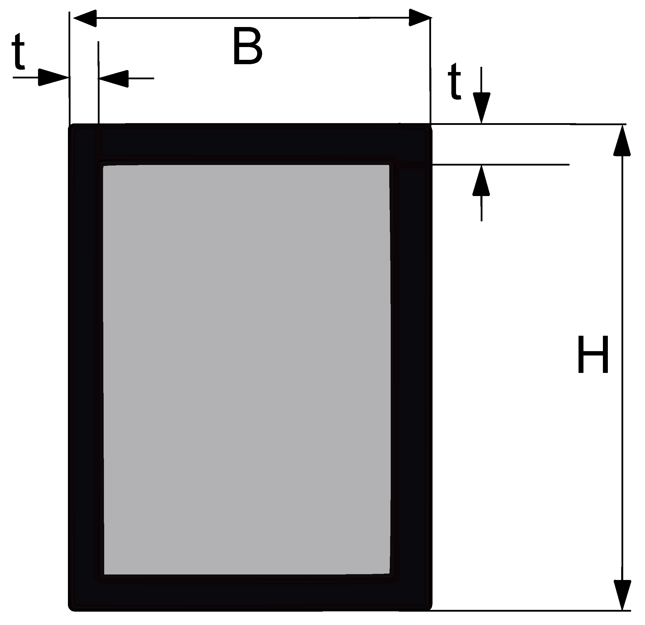In Equations (3) and (4), $D\prime$ is the equivalent diameter of the rectangular cross section calculated with $D^{\prime }=\sqrt{\left(B^2+H^2\right)}$, where $B$ and $H$ are the width and height of the cross section, respectively, as shown in Figure 1. The parameter $k_s$ in Equations (4) and (5) is the equivalent confining coefficient that incorporates the lack of concrete confinement due to the rectangular shape of the cross section into the equations. The parameter ranges for which Equations (1)–(5) are applicable are listed in

Table 2. Parameter ranges for which Equations (1) and (2) are applicable [7].

Width to thickness ratio	$12 \le B/t \le 100$
Height to Width ratio	$1 \le H/B \le 2$
Yield strength of the steel tube	$175 \mathrm{MPa} \le f_y \le 960 \mathrm{MPa}$
Compressive strength of the concrete	$20 \mathrm{MPa} \le f_c\prime \le 120 \mathrm{MPa}$
Steel wall thickness (mm)	$3 \le t \le 30$

.

Yan et al. [9] carried out an experimental program including the testing of 16 concentrically loaded square CFST stub columns under uniaxial compression. In these studies, ultra-high performance concrete classes have been used with compressive strengths ranging between 100 and 140 MPa. The yield stress in these experiments ranged between 445 and 670 MPa. All specimens possessed a side length of 100 mm and a $B/H$ ratio of 1. The thickness of the steel casing ranged between 4.9 and 18.5 mm. Wu et al. [10] studied the effect of increasing the column size on the compressive strength of the member since mostly larger sized members are used for practical applications compared to those tested in laboratory settings. Six CFST stub columns with square cross sections were tested under concentrically applied axial compressive loads. The side length of the square cross section ranged between 300 and 750 mm in these experiments. It was observed that as the size of the cross section increases, the favorable effect of confinement on the concrete core tends to decrease. Nguyen et al. 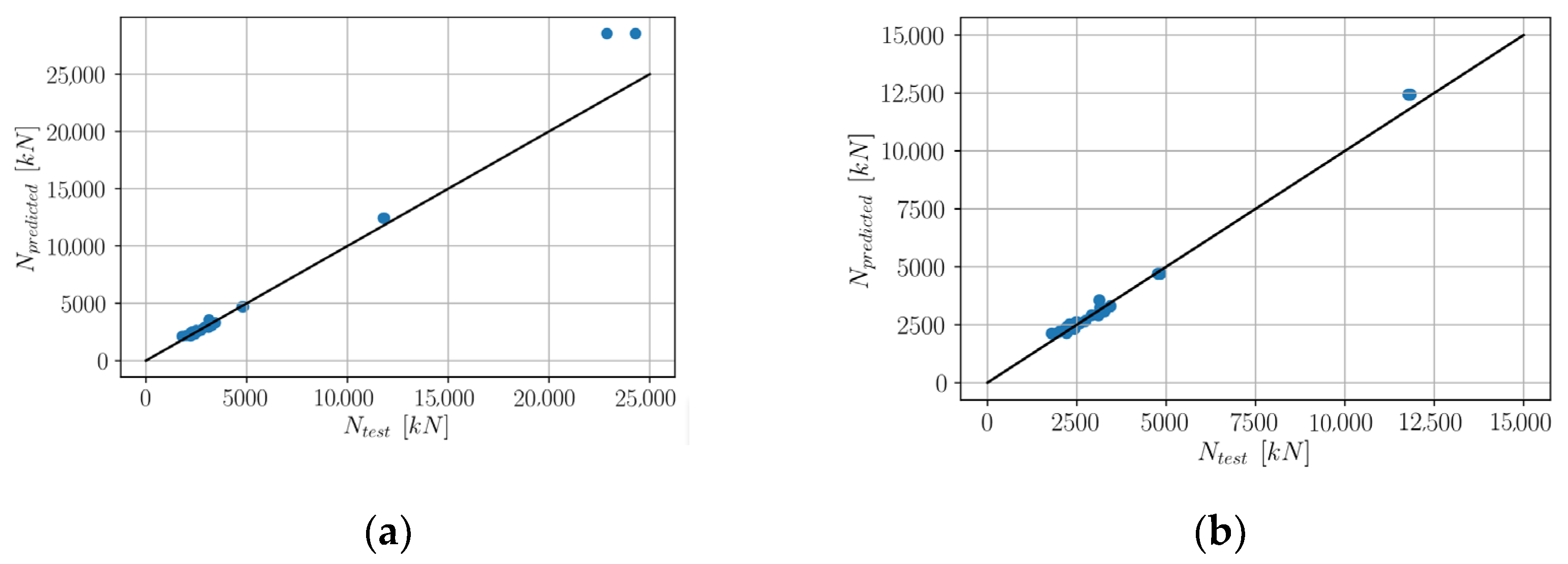[11] conducted an experimental program consisting of six CFST stub column specimens with square cross sections. Particularly, the cross sections were chosen to be slender. Uniaxial compressive loads were applied in a concentric manner. The equations proposed by Wang et al. [7] were applied to all of the specimens documented in [9,10,11]. The predicted ultimate loads are compared to the measured $N_u$ values in Figure 2. It was observed that a coefficient of determination of $R^2=0.94$ could be achieved by using Equations (1)–(5). Excluding the large-sized specimens with 750 mm side lengths, this coefficient could be increased to 0.99.

The current study deals with CFST stub columns with rectangular cross sections under uniaxial concentric loading conditions. The main objective of the study is to obtain design configurations that minimize CO₂ emissions associated with the production process of the structure while maintaining the compressive strength of the structure above a certain level. To this end, two different metaheuristic optimization techniques have been applied and their performances have been compared. The following Methods section contains the implementation procedure for these two algorithms. In addition to that, numerical examples are presented for both methods in Appendix. The optimized cross-sectional dimensions are tabulated for three different levels of concrete compressive strength in the Results section. The iteration processes are visualized for both optimization techniques at different ultimate load-carrying capacity levels. Most of the research investigations in the field of CFST columns have been focused on experimental testing and finite element modelling of these structures. The optimal design of CFST structures with respect to carbon emission is a mostly neglected field of research. The current study aims to draw attention to this important field because of its environmental significance.

2. Methods

Metaheuristic algorithms have been used on many challenging optimization problems. Metaheuristic techniques are based on the premise that natural phenomena such as the behavior of spider colonies are suitable for the optimization of engineering systems since these natural phenomena also tend to develop towards their optimum states. This assumption was warranted since many engineering systems could be successfully optimized by using metaheuristic techniques. Some of these techniques can be further improved by tuning the parameters they depend on. Particularly, these techniques are well known to converge to the global optima quickly and reliably without excessive computational effort. The metaheuristic algorithms most widely adopted in the field of engineering include harmony search algorithm [12,13], particle swarm optimization [14], artificial bee colony technique [15,16], ant colony algorithm [17], and Jaya algorithm [18]. In addition to metaheuristic techniques, cellular automata based methods have also been used in structural engineering optimization. Tajs-Zielinska and Bochenek [19] successfully applied cellular automata based techniques to the problem of structural topology optimization. The current study is focused on a newly proposed technique called social spider algorithm and its applicability relative to the optimization of CFST columns. Furthermore, the performance of this technique is compared to the time-tested methodology of harmony search optimization. The first application of the social spider optimization (SSO) to an engineering problem was by Alrashidi et al. [20]. In [20], the SSO technique is applied to the problem of wind speed characterization. Cakiroglu et al. [21] applied the SSO technique to the cost and ${\mathrm{CO}}_2$ emission optimization of CFST columns with circular cross sections. SSO was developed by Cuevas et al. [22].

2.1. Social Spider Optimization

The algorithm takes its name from a spider species called the social spider. This spider species dwell in colonies consisting of male and female spiders. The males in these colonies are further classified as dominant and non-dominant males [23]. The SSO algorithm mimics the interactions of these three different groups of social spiders to solve optimization problems. In this algorithm, a spider represents a solution candidate that can be a set of $N$ real numbers where $N$ is the number of variables being optimized. After the random generation of an initial population of solution candidates within predefined variable ranges, gender is assigned to each solution candidate. In the next phase of the algorithm, the entire population moves towards an overall better performing configuration based on certain rules defined with Equations (6)–(11).

$$w_i=\frac{F\left(s_i\right)-F\left(s_{worst}\right)}{F\left(s_{best}\right)-F\left(s_{worst}\right)}$$

(6)

$$I_{i,j}=w_j\cdot e^{-d_{i,j}{ }^2}$$

(7)

$$f_i^{k+1}=\left\{\begin{array}{c}{f}_i^k+\alpha I_{i,c}\left(s_c-f_i^k\right)+\beta I_{i,b}\left(s_b-f_i^k\right)+\delta \left(\gamma -\frac{1}{2}\right) for \epsilon <PF\\ f_i^k-\alpha I_{i,c}\left(s_c-f_i^k\right)-\beta I_{i,b}\left(s_b-f_i^k\right)+\delta \left(\gamma -\frac{1}{2}\right) for \epsilon \ge PF\end{array}\right.$$

(8)

$$WMM=\frac{{{\displaystyle \sum }}_{h=1}^{N_m}{m}_h^k{w}_{N_f+h}}{{{\displaystyle \sum }}_{h=1}^{N_m}{w}_{N_f+h}}$$

(9)

$$m_i^{k+1}=\left\{\begin{array}{c}{m}_i^k+\alpha I_{i,f}\left(s_f-m_i^k\right)+\delta \left(\gamma -\frac{1}{2}\right) for w_{N_f+i}>w_{N_f+m}\\ m_i^k+\alpha \left(WMM-m_i^k\right) for w_{N_f+i}\le w_{N_f+m}\end{array}\right.$$

(10)

$$r=\frac{{{\displaystyle \sum }}_{j=1}^n(v_j^{high}-v_j^{low})}{2n}$$

(11)

In order to classify the spiders according to their fitness, a weight is assigned to each solution candidate, as shown in Equation (6), where $F\left(s_i\right)$ denotes the fitness of the solution candidate with the index $i$. The fitness function plays a crucial role in this optimization process. In the case of CO₂ emission minimization, $F$ can be a function that returns the amount of CO₂ emission associated with a solution candidate $s_i$. Consequently, solution candidates with lower CO₂ emissions also have better fitness and greater weight. Since the fitness of $s_i$ is inversely proportional to the amount of CO₂ emissions, $F\left(s_i\right)$ can also return the inverse of the mass of CO₂ associated with $s_i$ so that better fitness is reflected in Equation (6) as $w_i$ becomes greater. An illustration of the development of a randomly generated population by using Equations (6)–(11) can be observed in Appendix A.

The spiders are attracted or repelled by each other in proportion to the intensity of the vibrations they receive from each other. These intensities are calculated using Equation (7), where $d_{i,j}$ is the Euclidean distance between the solution candidates with the indices $i$ and $j$. Equations (8) and (10) show the female and male iteration steps, respectively. In Equation (8), $f_{î}^{k+1}$ is the state of a female spider (solution candidate) after the updates, and $m_{î}^{k+1}$ is the updated state of a male spider in Equation (10). 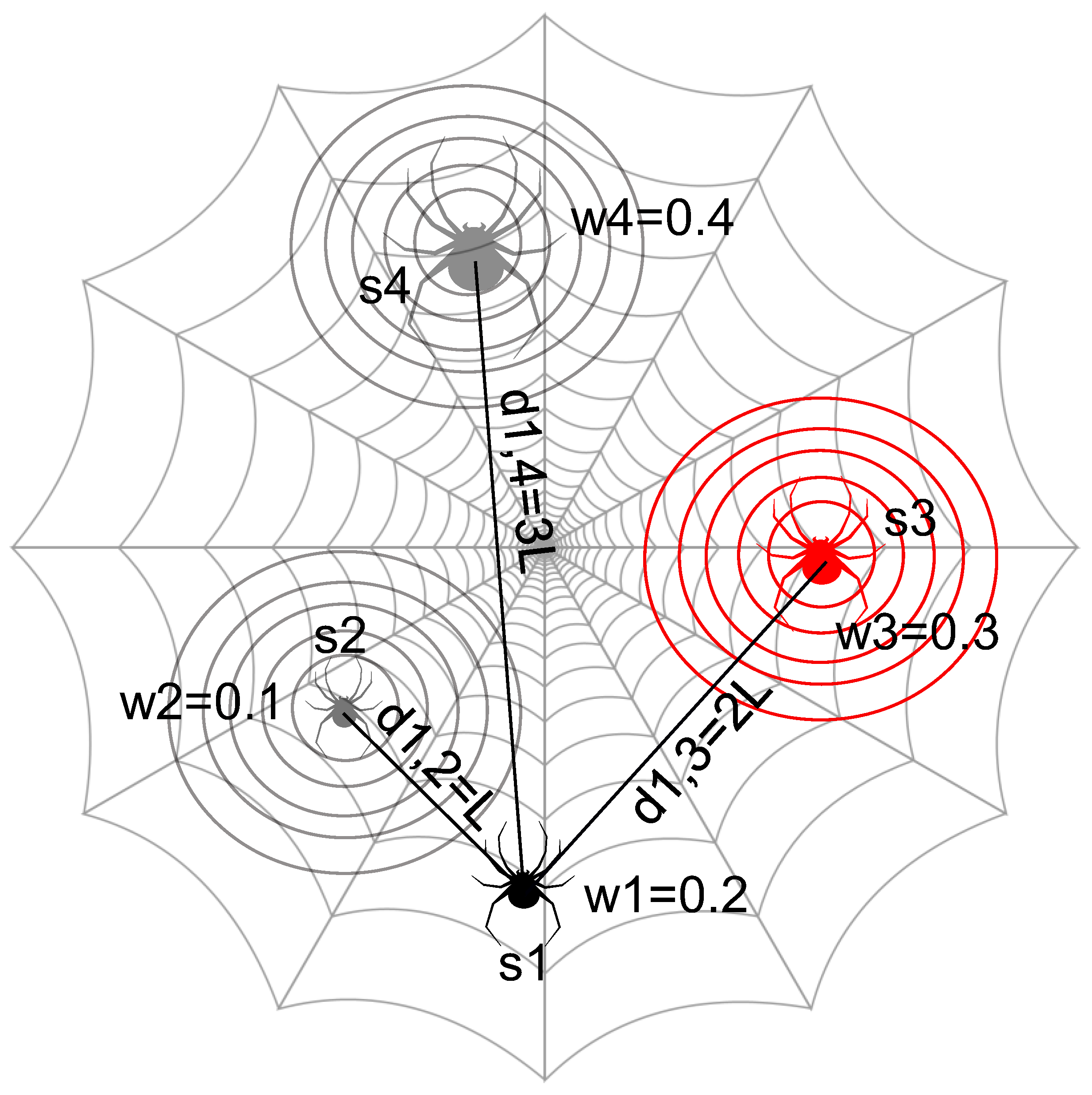In these equations, $\alpha , \beta , \gamma , \mathrm{and} \delta$ are random numbers between zero and one. As Equation (8) shows, the female spider update steps consist of three different components. The first of these components is the attraction of the female spider towards the nearest spider in the colony that also performs better. The vibration intensity of this spider is denoted with $I_{i,c}$. This kind of attraction is also visualized in Figure 3. The next component of the female spider update is the attraction towards the best-performing member in the entire colony, and its vibration intensity is denoted by $I_{i,b}$. The third component of the female iteration is a random movement represented by the $\delta \left(\gamma -\frac{1}{2}\right)$ term. The second line of Equation (8) represents the case in which the female spider $f_i$ is repelled by the nearest better-performing and best-performing members of the colony, which may occur depending on the value of the variable $\epsilon$. In each iteration, $\epsilon$ is assigned a new value between zero and one which is compared to the threshold value $PF$. Here, $PF$ takes values between zero and one and higher values of $PF$ in order to have a greater probability of attraction instead of repulsion of the female spider as a consequence. In Equation (10), the first line of the equation describes the attraction of a dominant male spider towards the nearest female in the colony. On the other hand, the second line describes the movement of a non-dominant male towards the weighted mean of the entire male population, which is denoted by $WMM$. In Equation (9), $N_f$ and $N_m$ are the total numbers of female and male spiders in the colony, respectively. 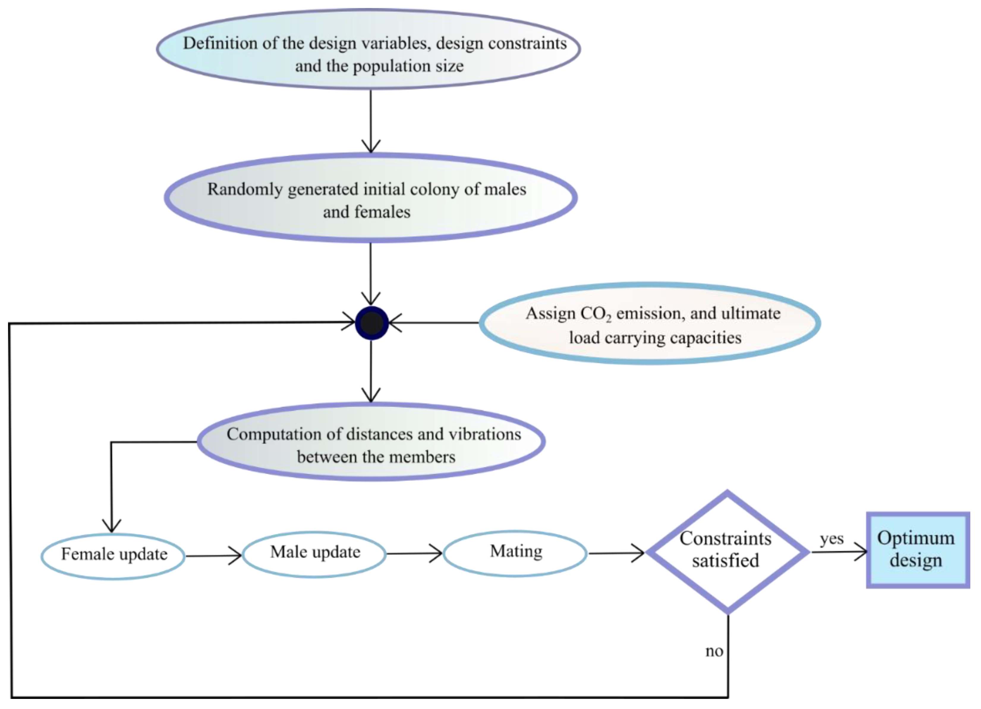In Equation (10), $s_f$ denotes the nearest female spider to $m_i$, and $w_{N_f+m}$ is the weight of the median member of the male population. The addition of new members to the colony happens through the mating process in which dominant males mate with female spiders within their radius of mating. In Equation (11), r denotes the radius of mating. Here, $v_j^{high}$ and $v_j^{low}$ are the upper and lower bounds of the j-th design variable, and n is the total number of design variables. The spiders that are involved in mating influence the properties of the newly generated spiders in proportion to their weights. Depending on their quality, the newly generated spiders either replace the worst-performing spiders in the population or are discarded. A flowchart of the social spider algorithm is provided in Figure 4. Further details about this algorithm can be found in [21].

2.2. Harmony Search Algorithm

A metaheuristic algorithm that found application in diverse areas of engineering is the harmony search technique that was invented by Geem [12]. Initially conceived for the optimization of discrete-valued data, the technique eventually evolved in such a manner that it applies to a wide range of problems including water network design [24,25], analysis of plane stress systems [26], design of retaining walls [27], vehicle routing [28], and stacking sequence optimization of laminated composite plates [29].

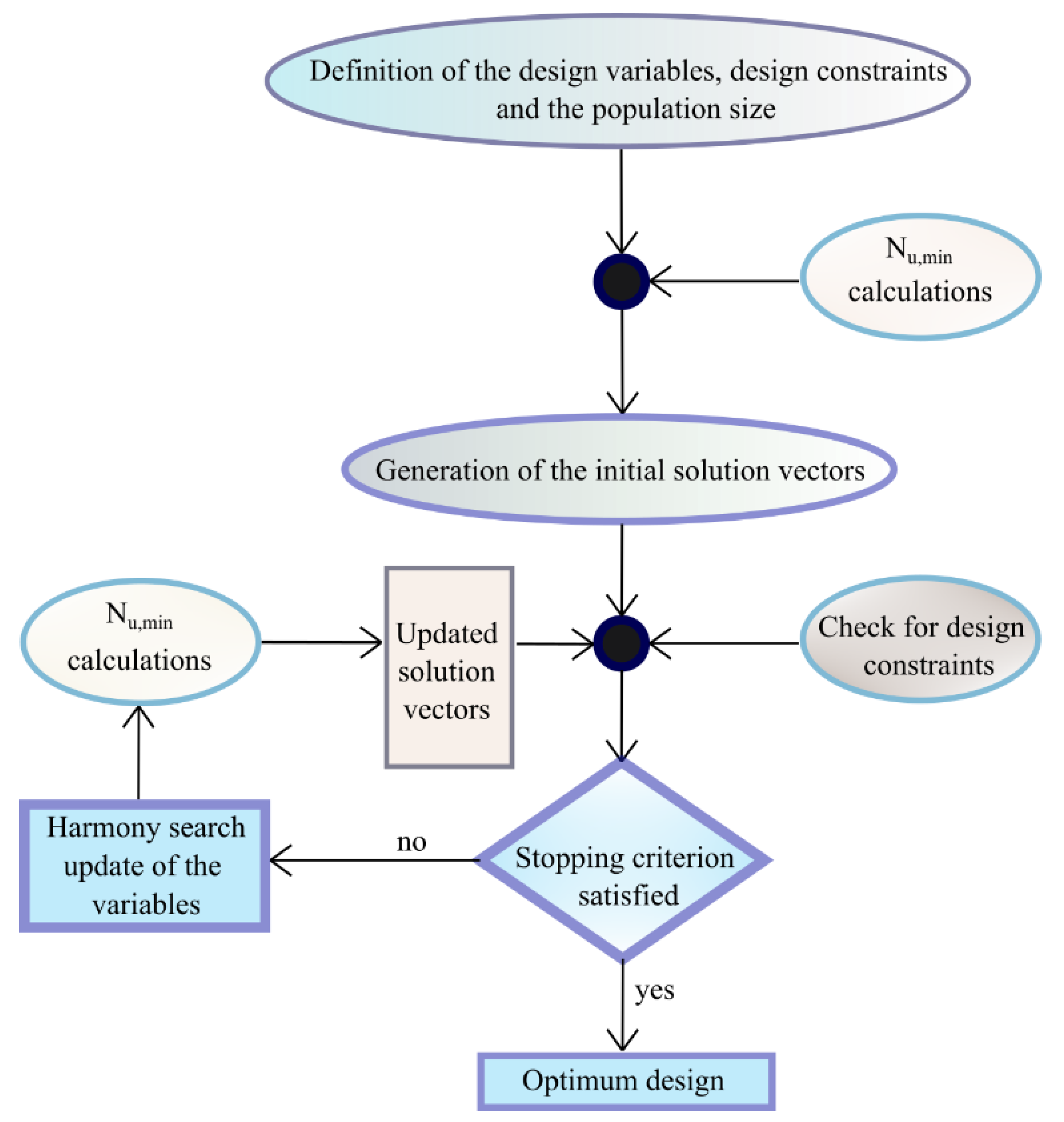
The starting point of harmony search optimization is the choice of the design parameters and the objective function. In the case of rectangular CFST columns, these design variables are the side lengths of the column cross section. In this study, the objective quantity to be minimized was chosen to be the CO₂ emission associated with manufacturing the columns. The goal of the study is to determine the best type of column cross section based on CO₂ emissions associated with different design configurations. Once the design parameters are chosen, an initial set of parameter vectors has to be generated randomly while considering the optimization constraints. This set of randomly generated design parameters constitutes an initial population that is expected to move towards an optimum solution through the harmony search iterations. After each iteration step, the members of the population are ranked according to their performance (in this case, the CO₂ emission). The newly generated parameter vectors are compared to the existing members of the population, and they replace the worst-performing member in the case where they perform better than some of the existing population members. The harmony search iterations are repeated until the newly generated members no longer exhibit significant improvements compared to the existing population members.

The parameters that play a decisive role in the harmony search iterations are the harmony memory consideration rate $\left(HMCR\right)$ and the pitch adjustment rate $\left(PAR\right)$. These parameters take different values in each iteration step and are calculated as $HMCR=0.5 \ast \left(1-iter/maxiter\right)$ and $PAR=0.05 \ast \left(1-iter/maxiter\right)$. Here, $iter$ stands for the index of the current harmony search iteration, and $maxiter$ stands for the maximum number of iterations. Equation (12) shows the computation steps for the newly generated member of the population using $HMCR$ and $PAR$.

$$\begin{gathered} k=\left[int\right]\left(rand\ast HMS\right), \\ {x}_{i,new}=\left\{\begin{array}{c}{x}_{i,min}+rand\times \left(x_{i,max}-x_{i,min}\right), if HMCR>rand\\ x_{i,k}+rand2\ast PAR\times \left(x_{i,max}-x_{i,min}\right), if HMCR\le rand\end{array}\right. \end{gathered}$$

(12)

In Equation (9), $rand\in \left(0,1\right)$ and $rand2\in \left(-1/2,1/2\right)$; $HMS$ is the total number of parameter vectors in the population; $x_{i,k}$ is the $i-th$ design variable in the $k-th$ member in the population of parameter vectors; $k$ is the integer value nearest to the product $rand\ast HMS$; and $x_{i,min}$ and $x_{i,max}$ are the minimum and maximum values of the variable with the index $i$ in a parameter vector, respectively.

In the initial step of randomly populating the design vectors as well as in the subsequent iteration steps, certain constraints need to be imposed on the design variables. In addition to the parameter ranges listed in Table 2, the constraint of minimum ultimate load-carrying capacity $\left(N_{u,min}\right)$ was placed on each design vector such that, throughout the optimization process, only the design configurations that satisfy certain predetermined load carrying capacity requirements were accepted as valid design configurations. A flow chart of this algorithm is provided in Figure 5. A numerical example of the harmony search algorithm can be found in Appendix B.

3. Results

CO₂ emissions were optimized based on the concrete classes like C25, C40, and C60. The ultimate axial load capacity $\left(N_{u,min}\right)$ is set for each class and used as optimization constraints with the constraints of the cross-section areas. By using the harmony search and social spider algorithms, the cross-sectional width and height of the member are optimized while keeping $N_u$ above the threshold value at all times. The cross-sectional dimensions that do not satisfy the $N_{u,min}$ constraints are discarded during the harmony search and social spider iterations. In these optimizations, the cross-sectional height $\left(H\right)$ and width $\left(B\right)$ are the optimization variables such that modifying these dimensions results in different volumes of concrete and steel used in the manufacturing of the CFST stub columns which, in turn, results in different amounts of CO₂ emission. For both techniques, the optimization process has been repeated at six different levels of the tube wall thickness and four different levels of the axial load carrying capacity for the concrete classes C25, C40, and C60. 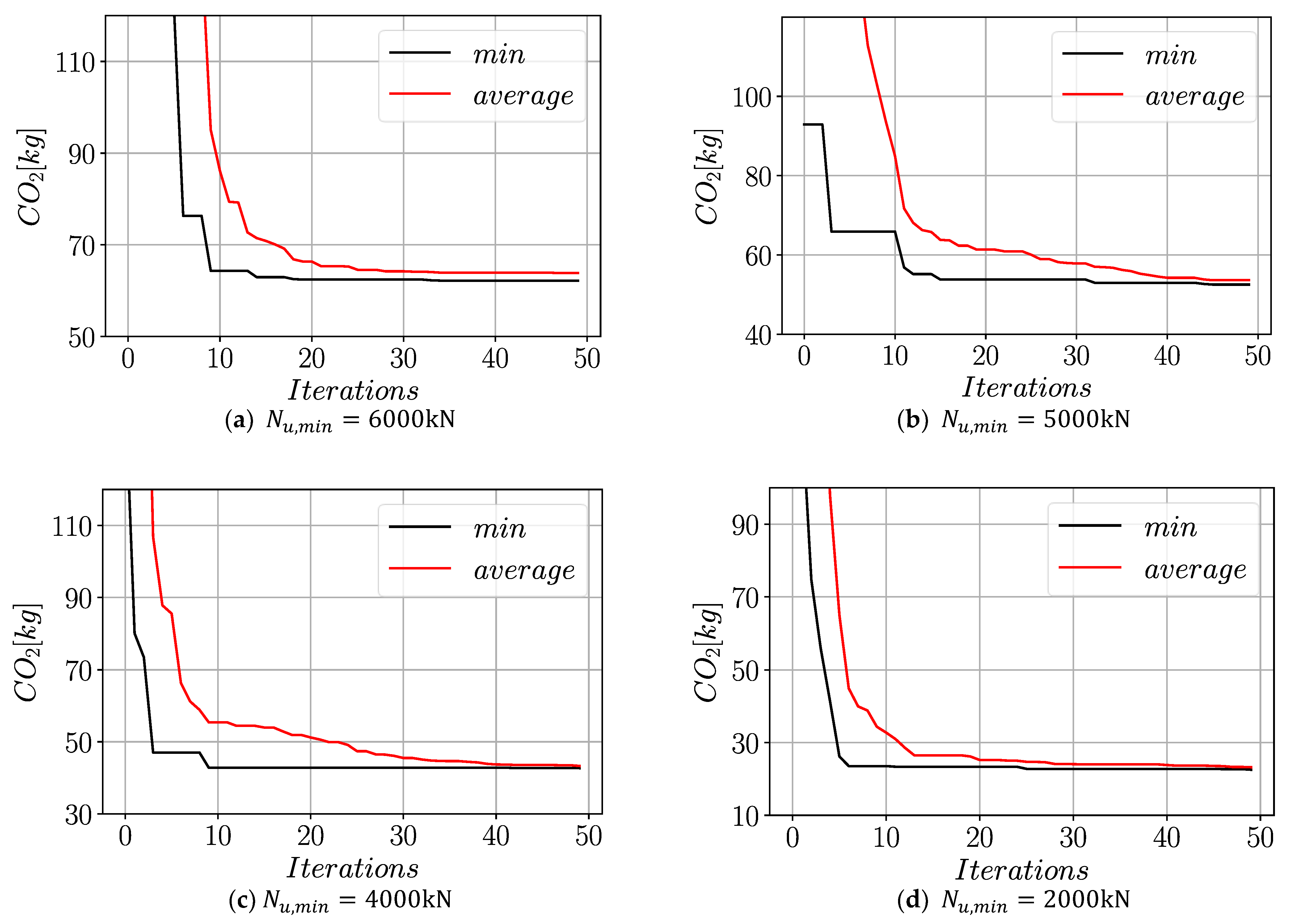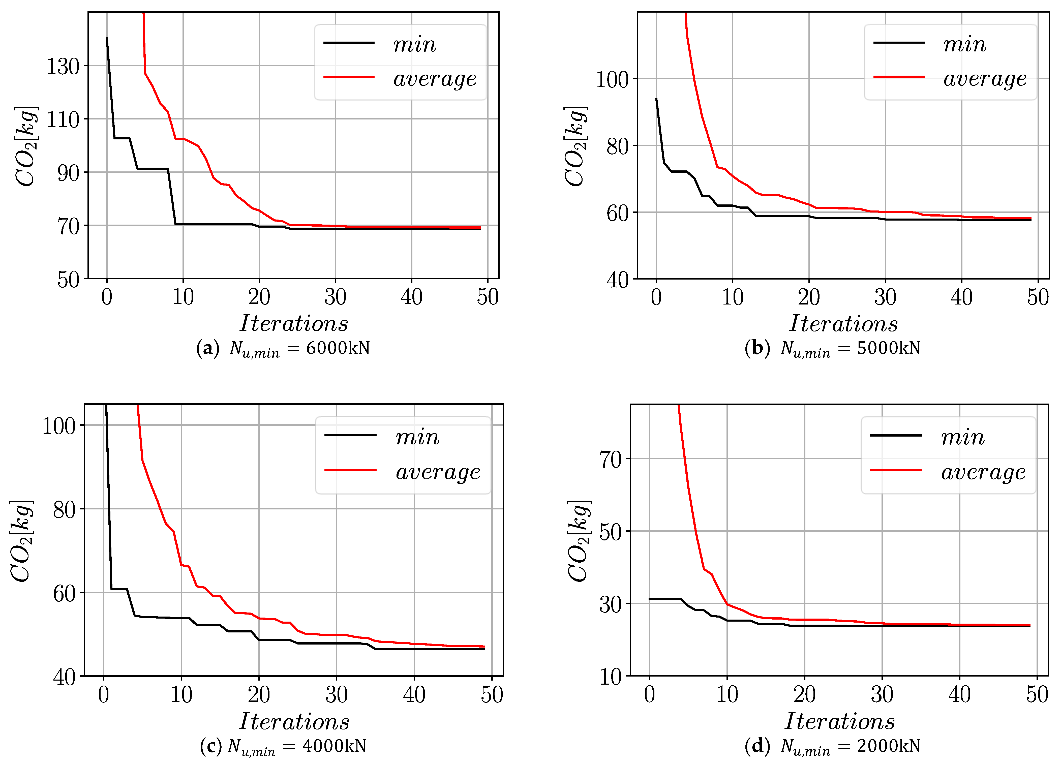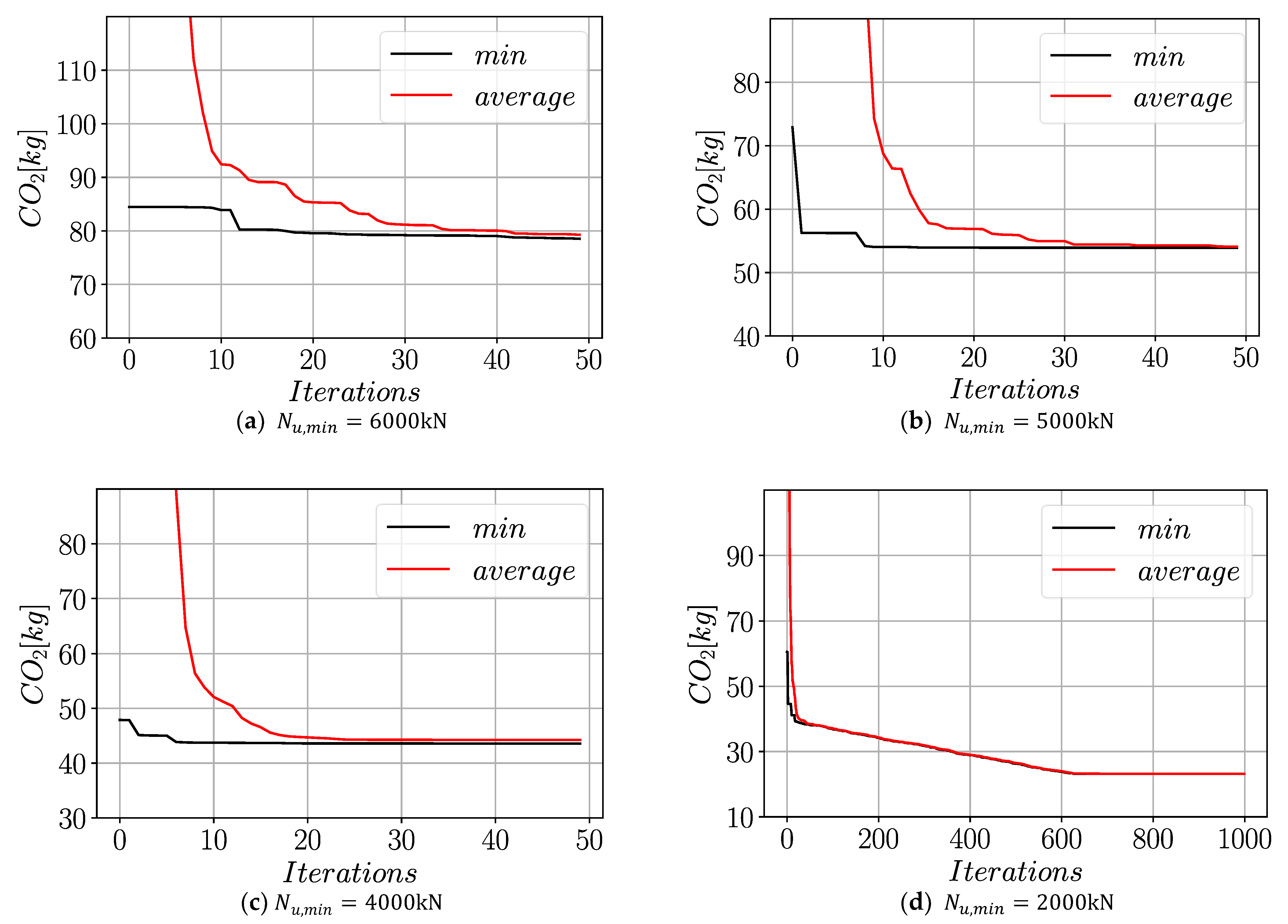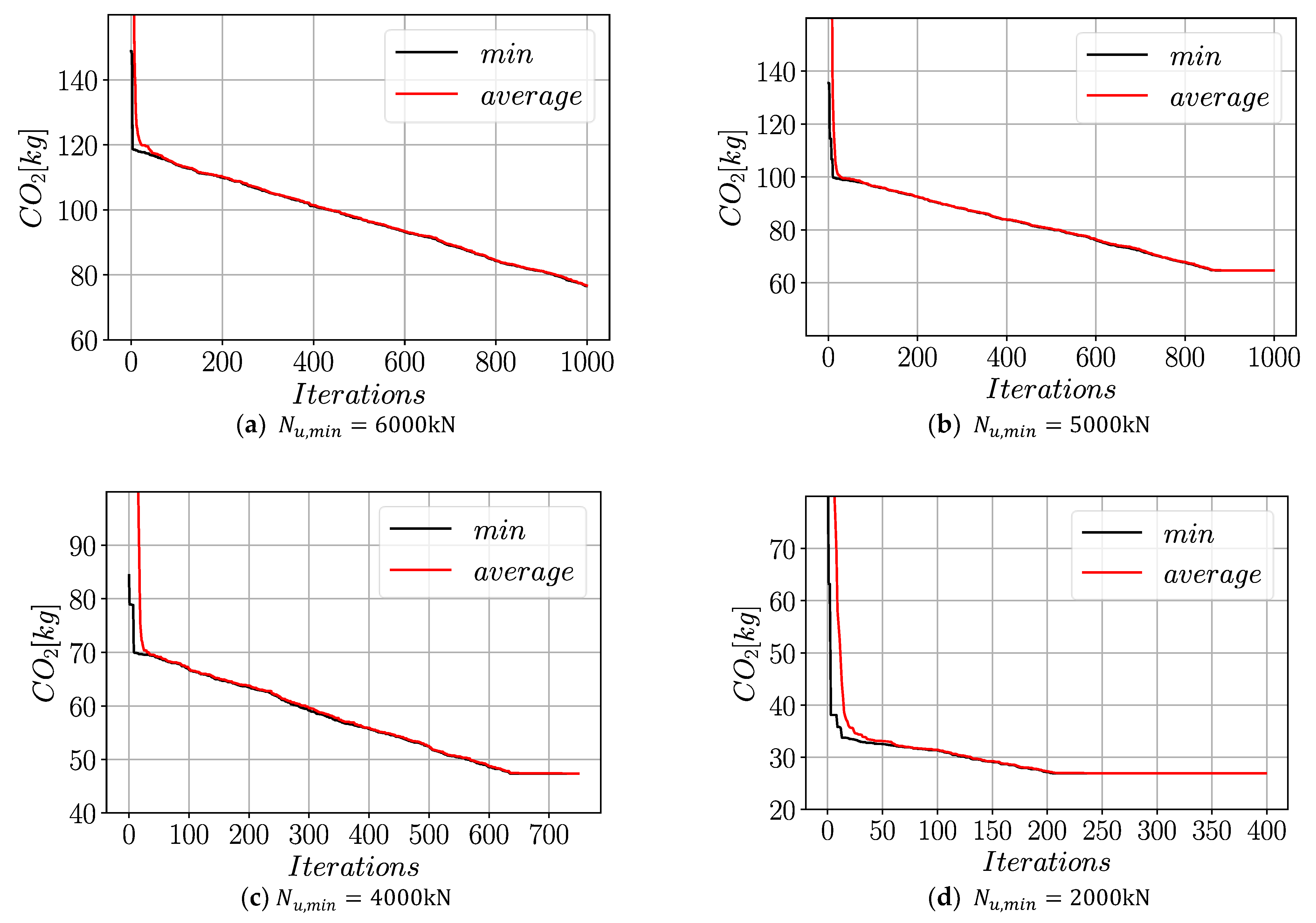As the optimization objective, the CO₂ emission associated with the production of a CFST stub column with unit height is selected. The results obtained from both the harmony search and social spider algorithms are visualized in the following sections. In Figure 6, the results of the harmony search optimization process are presented at four different levels of ultimate load carrying capacity for rectangular columns with concrete class C25 and the wall thickness kept constant at 5 mm. The black and red curves in Figure 6 indicate the minimum and average CO₂ emissions, respectively, in the entire population of solution candidates at each iteration step. From Figure 6, it is clear that less than fifty harmony search iterations were sufficient to observe a convergence of the minimum CO₂ emission at all $N_{u,min}$ levels. Moreover, at each level of $N_{u,min}$, the average CO₂ emission converges towards the minimum CO₂ emission curve within the first fifty iterations. The optimum CO₂ emissions as well as the corresponding cross-sectional dimensions are listed in

Table 3. Minimum CO₂ emissions for rectangular cross section obtained from harmony search optimization.

Concrete Class	Nu,min (kN)	Min. CO2 Emission (kg)	H (mm)	B (mm)	T (mm)	B/H
C25	6000	62.1	310	245	5	0.79
	5000	52.4	268	205	5	0.77
	4000	42.7	224	165	5	0.74
	2000	22.4	127	84	5	0.66
C40	6000	67.8	268	225	5	0.84
	5000	56.6	236	191	5	0.81
	4000	45.5	201	157	5	0.78
	2000	23.2	119	84	5	0.71
C60	6000	74.6	238	201	5	0.85
	5000	61.3	209	176	5	0.84
	4000	48.4	183	144	5	0.79
	2000	23.7	110	83	5	0.76
C25	6000	65.2	253	177	7	0.70
	5000	55.1	218	148	7	0.68
	4000	44.7	180	120	7	0.67
	2000	23.3	100	63	7	0.63
C40	6000	68.7	229	174	7	0.76
	5000	57.5	199	147	7	0.74
	4000	46.3	169	120	7	0.71
	2000	23.6	97	65	7	0.67
C60	6000	71.8	209	165	7	0.79
	5000	59.5	181	144	7	0.80
	4000	47.4	157	116	7	0.74
	2000	23.6	93	65	7	0.70
C25	6000	67.5	212	142	9	0.67
	5000	56.9	181	120	9	0.66
	4000	46.2	152	96	9	0.63
	2000	24	83	54	9	0.65
C40	6000	69.6	199	142	9	0.71
	5000	58.3	174	120	9	0.69
	4000	46.9	144	99	9	0.69
	2000	24.0	82	55	9	0.67
C60	6000	71	187	139	9	0.74
	5000	59.1	162	120	9	0.74
	4000	47.3	137	99	9	0.72
	2000	24.1	80	56	9	0.70
C25	6000	69.2	185	119	11	0.64
	5000	59.1	158	101	11	0.64
	4000	47.2	130	84	11	0.65
	2000	24.3	74	49	11	0.66
C40	6000	70.4	177	122	11	0.69
	5000	59.0	153	103	11	0.67
	4000	47.4	128	84	11	0.66
	2000	24.6	74	49	11	0.66
C60	6000	70.9	169	121	11	0.72
	5000	59.1	146	104	11	0.71
	4000	47.6	123	87	11	0.71
	2000	24.7	72	51	11	0.71
C25	6000	70.6	163	106	13	0.65
	5000	59.4	140	90	13	0.64
	4000	47.9	116	75	13	0.65
	2000	25.0	67	46	13	0.69
C40	6000	71.2	160	106	13	0.66
	5000	59.5	138	91	13	0.66
	4000	48.0	115	77	13	0.67
	2000	25.2	67	47	13	0.70
C60	6000	71.1	154	108	13	0.70
	5000	59.7	134	93	13	0.69
	4000	48.2	112	78	13	0.70
	2000	25.3	66	48	13	0.73
C25	6000	71.5	148	96	15	0.65
	5000	60.0	128	82	15	0.64
	4000	48.5	107	70	15	0.65
	2000	25.6	63	45	15	0.71
C40	6000	71.8	146	98	15	0.67
	5000	60.4	127	84	15	0.66
	4000	49.0	106	71	15	0.67
	2000	25.9	63	46	15	0.73
C60	6000	71.9	143	98	15	0.69
	5000	60.5	125	85	15	0.68
	4000	49.1	104	73	15	0.70
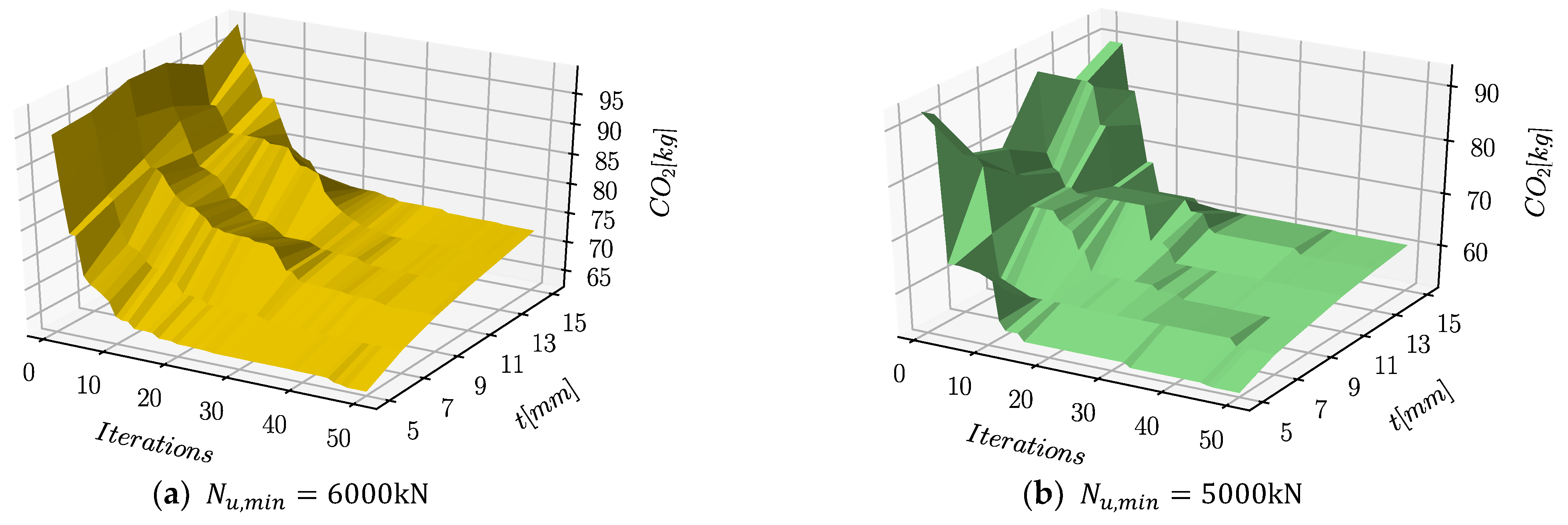
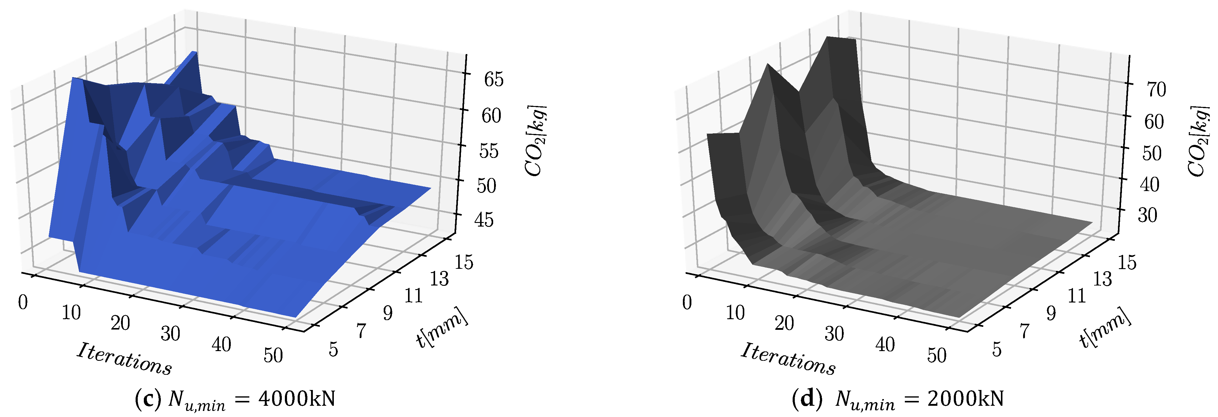
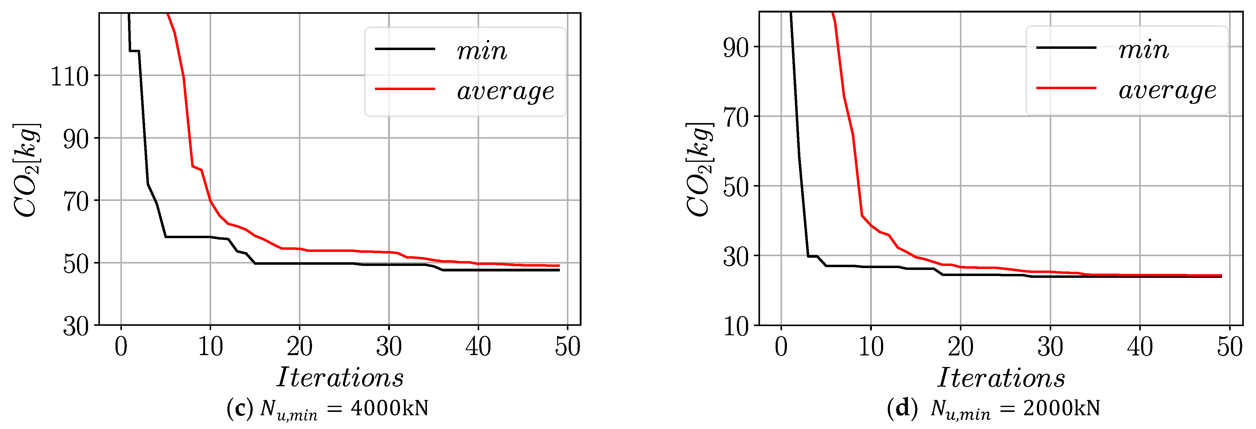
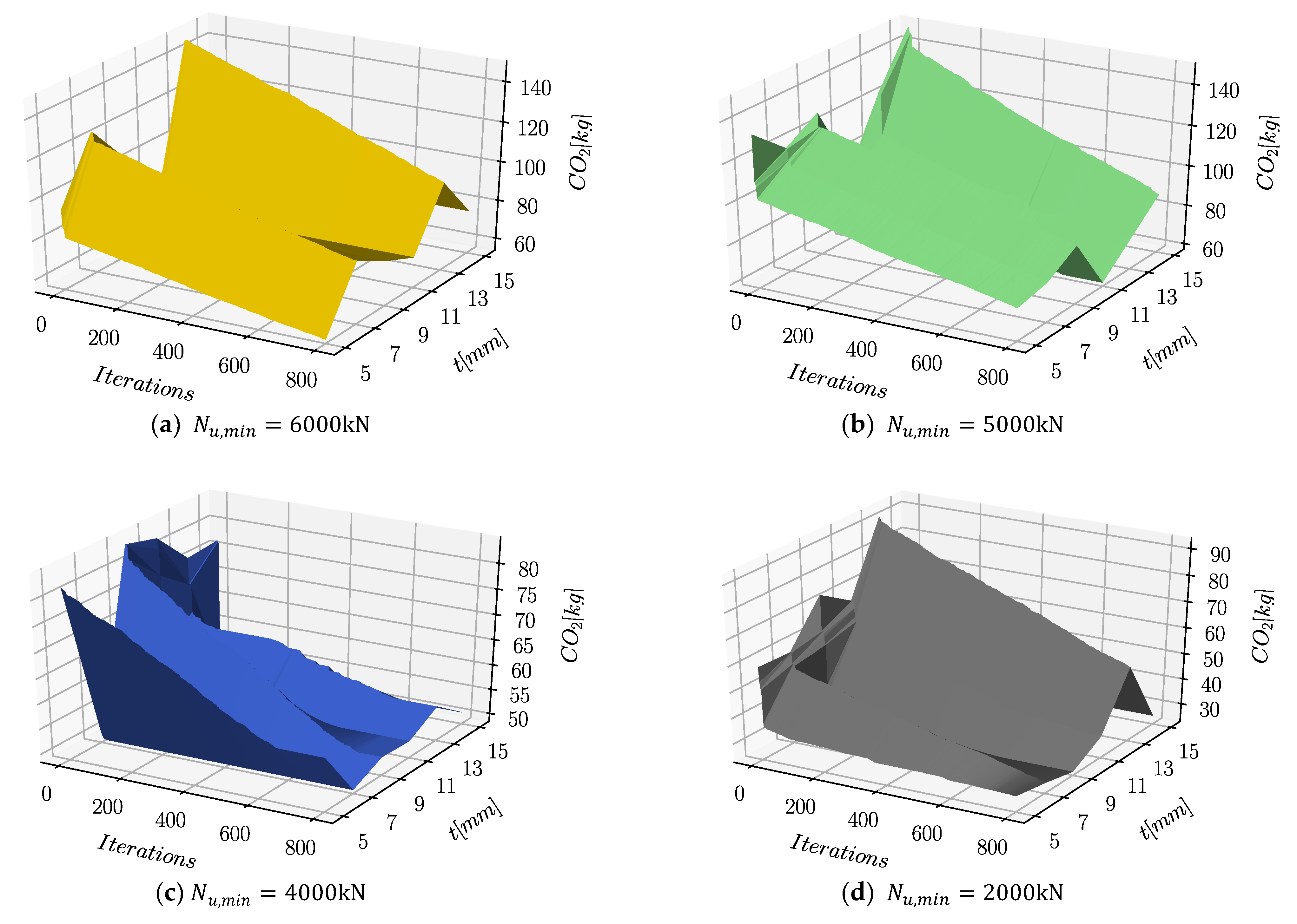
	2000	26.0	62	47	15	0.76

. In all optimizations, the steel tube’s yield strength was kept constant at 800 MPa. In order to visualize the variations in the optimization process for all levels of wall thickness, three-dimensional surface plots were generated at each level of $N_{u,min}$. Figure 7 shows the surface plots for the concrete class C25. These surface plots show a slight increase in CO₂ emissions as the wall thickness increases towards 15 mm.

Similar to Figure 6, Figure 8 and Figure 9 show the minimum and average CO₂ emission curves for C40 and C60 concrete classes and t = 7 mm and t = 9 mm wall thicknesses, respectively. Furthermore, Figure 10 and Figure 11 show three-dimensional surface plots of CO₂ emissions for these concrete classes. In all of these optimization attempts, the harmony search algorithm was able to reach convergence to a minimum CO₂ emission value in less than 50 iterations. By using the harmony search optimization, average minimum CO₂ emissions of 48.8 kg, 50.0 kg, and 51.1 kg could be achieved for C25, C40, and C60 concrete classes, respectively. A comparison of the values listed in Table 3 for different levels of $N_{u,min}$ shows that as the requirement for the $N_{u,min}$ increases so does the corresponding CO₂ emission. Furthermore, increased concrete strength results in greater CO₂ emissions. As listed in Table 1, concrete classes with higher strength are associated with more increased CO₂ release. According to Table 3, the B/H ratio of the optimum configurations varies between 0.6 and 0.85. The distribution of these ratios can be observed in Figure 12.

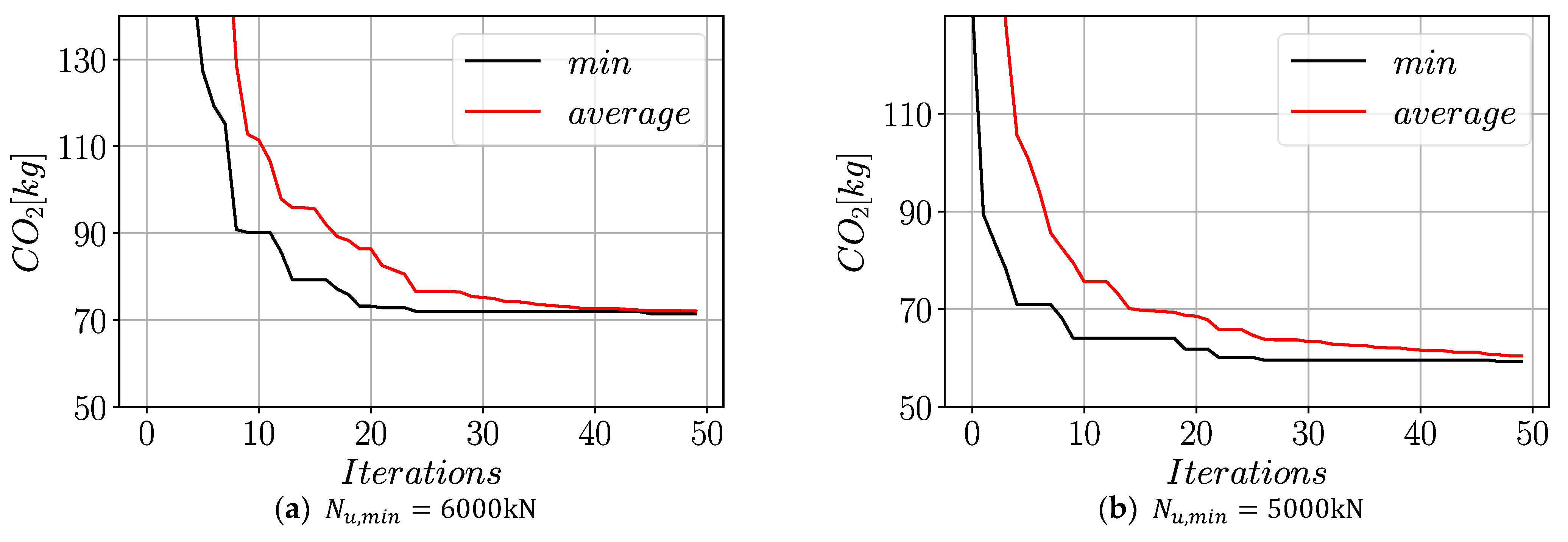
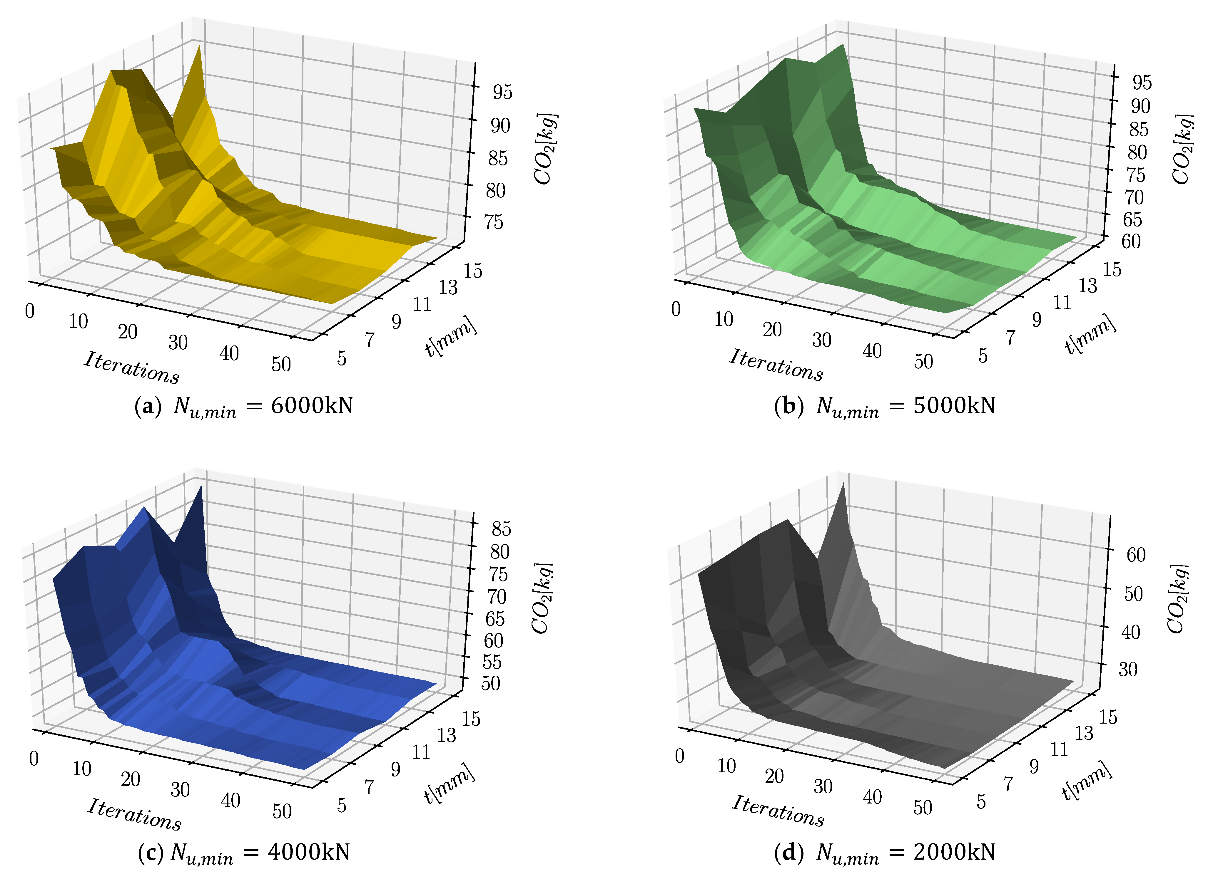
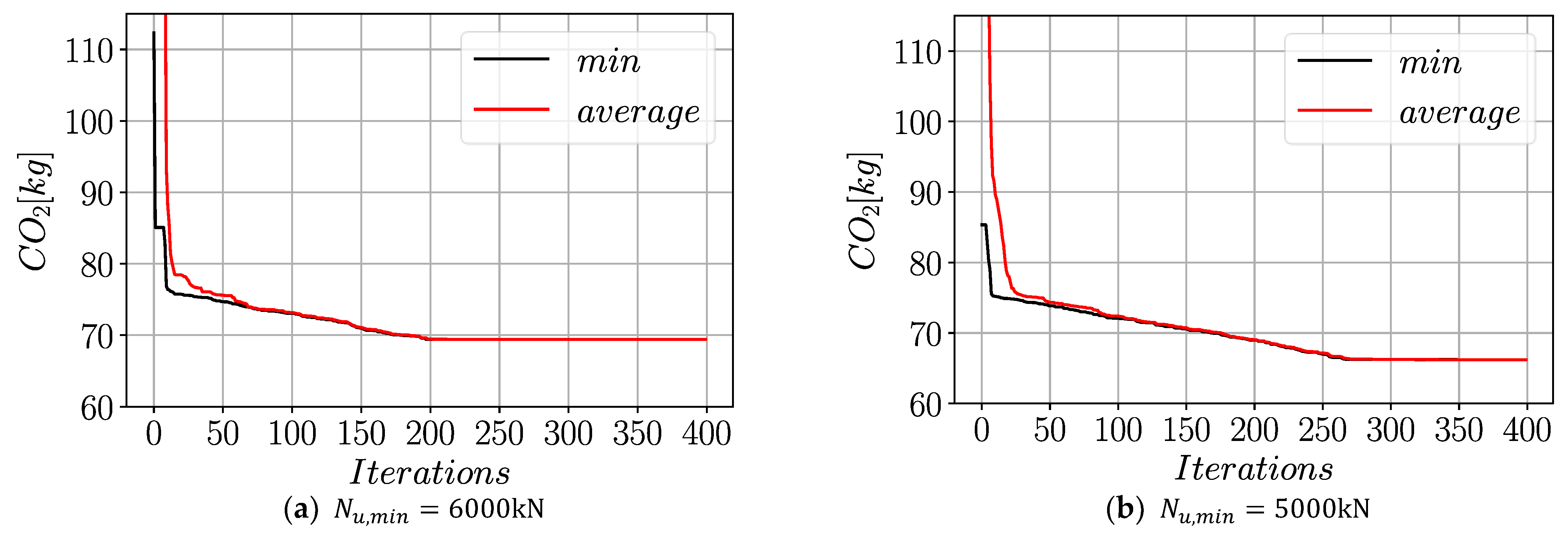
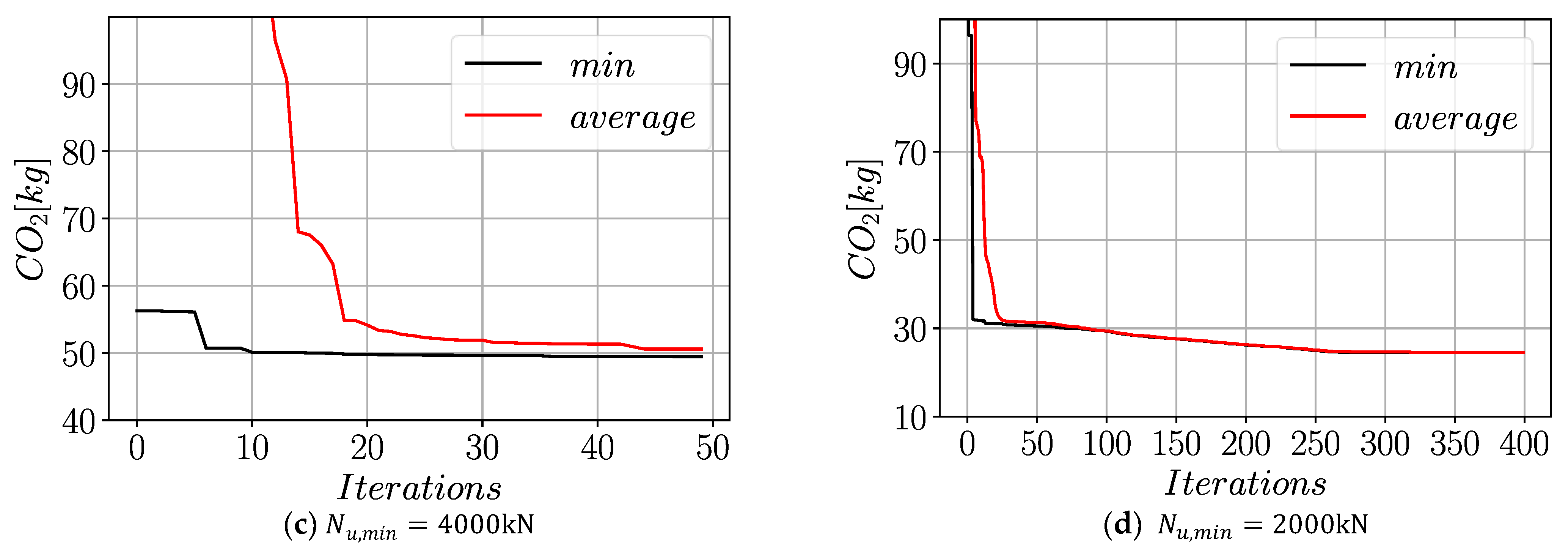
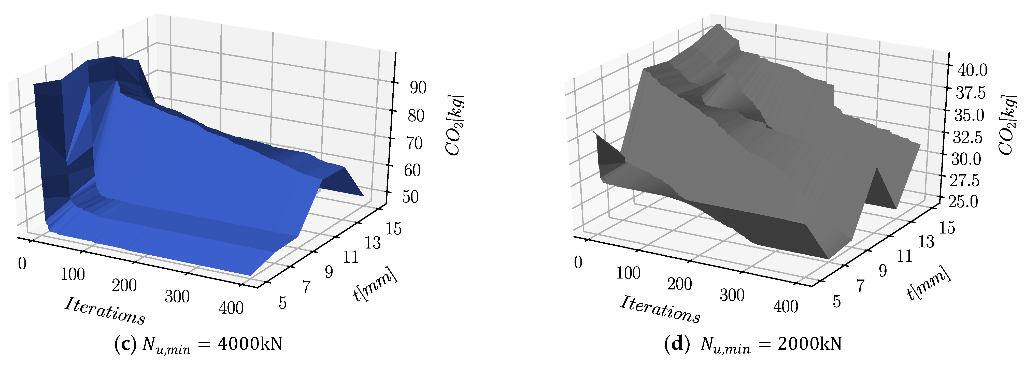
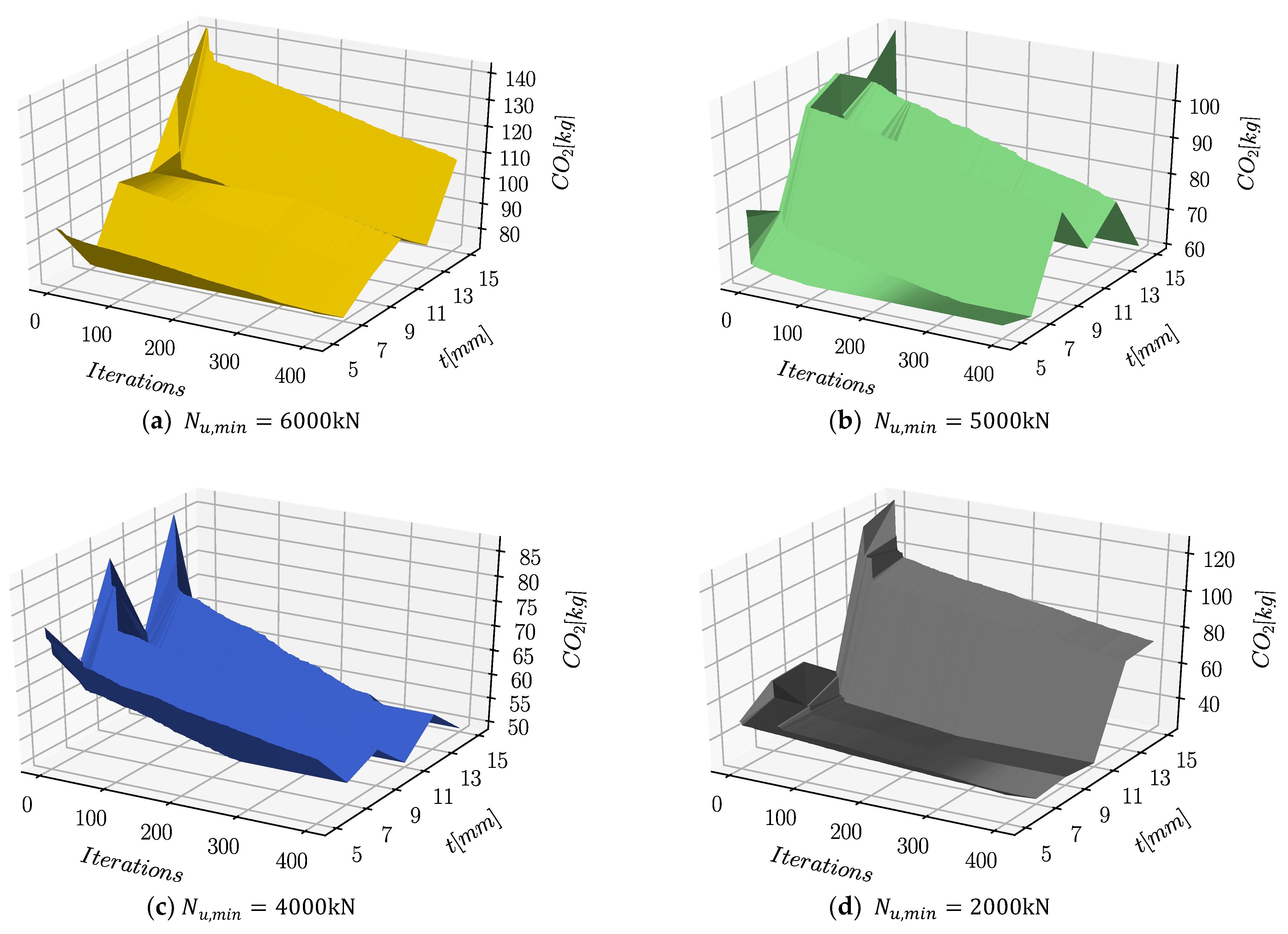
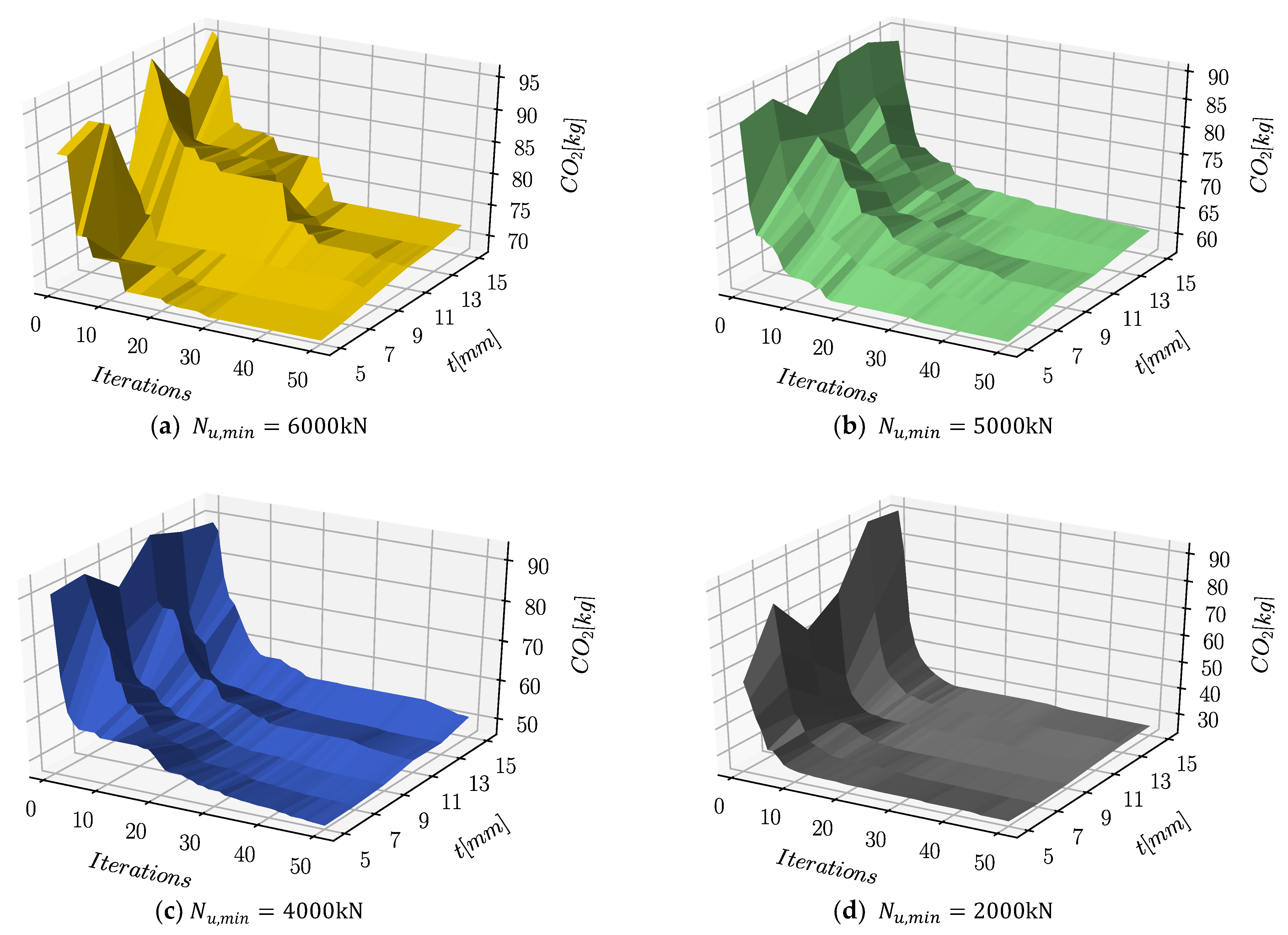
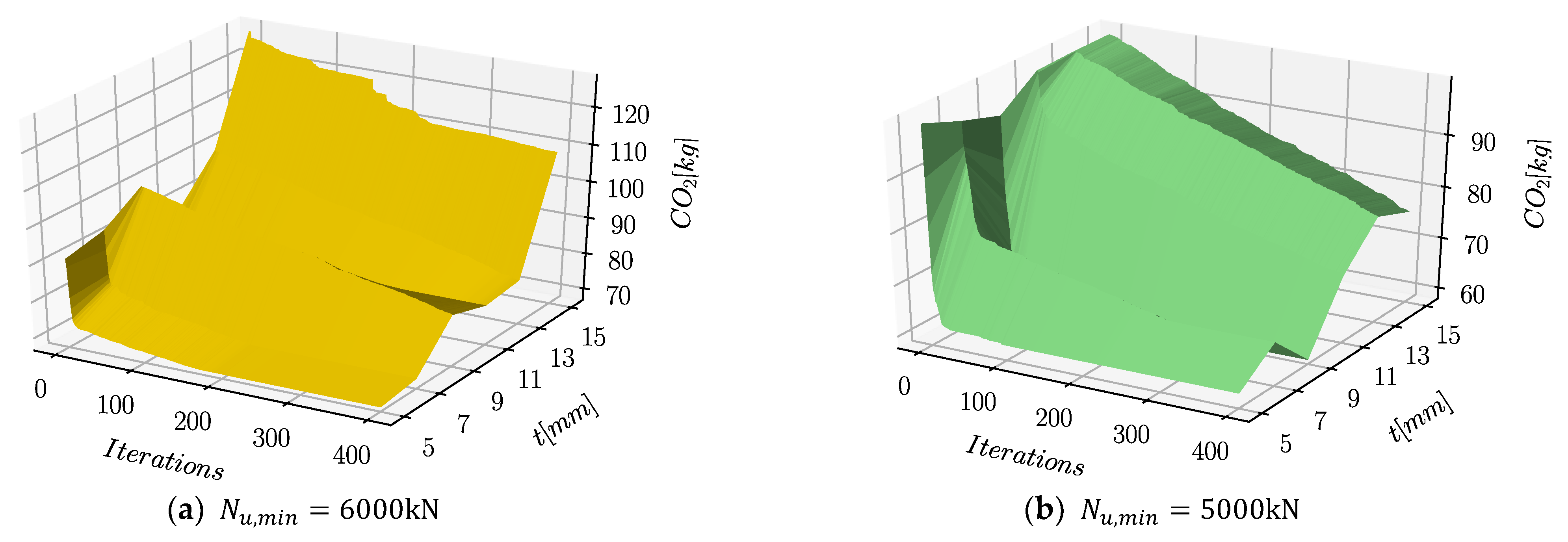
Figure 13, Figure 14 and Figure 15 show the outcome of social spider optimization for CFST stub columns with rectangular cross sections for C25, C40, and C60 concrete classes for the wall thicknesses t = 5 mm, t = 7 mm, and t = 9 mm, respectively. The corresponding surface plots of CO₂ emissions can be observed in Figure 16, Figure 17 and Figure 18. Although a quick convergence in less than 50 iterations could be observed in some of these optimization cases, in most cases a significantly larger number of iterations were necessary to obtain convergence to a minimum. 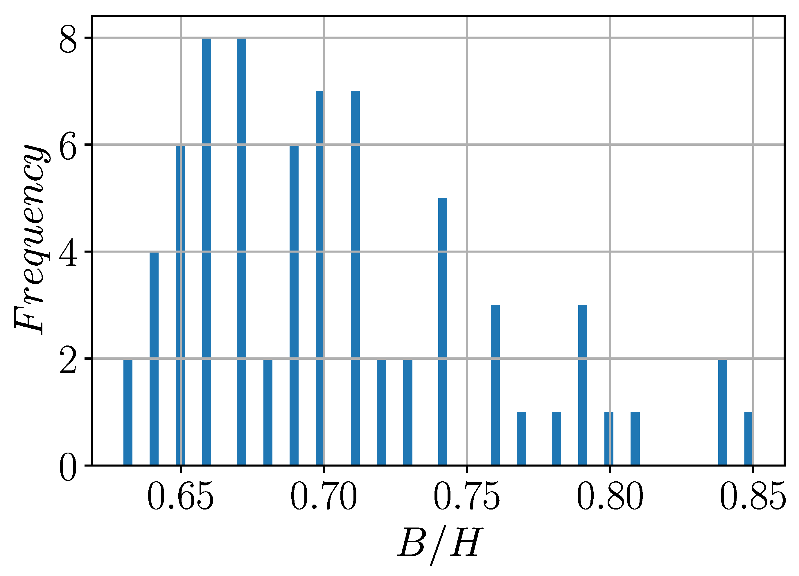Furthermore, the B/H ratios of the obtained optimum configurations did not present a regular pattern comparable to the harmony search results. A list of the optimized cross-sectional dimensions obtained from the social spider optimization of rectangular cross sections can be observed in

Table 4. Minimum CO₂ emissions for rectangular cross section obtained from social spider optimization.

Concrete Class	$$\begin{gathered} {\mathit{N}}_{\mathit{u},\mathit{m}\mathit{i}\mathit{n}} \\ \left(\mathbf{kN}\right) \end{gathered}$$	Min. CO2 Emission (kg)	H (mm)	B (mm)	T (mm)	B/H
C25	6000	65	342	233	5	0.68
	5000	53.9	280	202	5	0.72
	4000	43.6	199	190	5	0.96
	2000	23.2	153	72	5	0.47
C40	6000	67.8	253	238	5	0.94
	5000	60.6	435	111	5	0.26
	4000	46.5	285	113	5	0.40
	2000	27.1	325	36	5	0.11
C60	6000	75.2	229	211	5	0.92
	5000	62.4	234	158	5	0.68
	4000	48.6	189	140	5	0.74
	2000	24.2	116	80	5	0.69
C25	6000	69.4	358	133	7	0.37
	5000	55.5	214	152	7	0.71
	4000	49.1	230	103	7	0.45
	2000	24.3	103	64	7	0.62
C40	6000	71.8	294	137	7	0.47
	5000	66.2	455	74	7	0.16
	4000	50	259	85	7	0.33
	2000	24.6	100	66	7	0.66
C60	6000	73.3	282	125	7	0.44
	5000	59.7	200	131	7	0.66
	4000	52.8	309	66	7	0.21
	2000	25.3	112	42	7	0.38
C25	6000	76.6	307	111	9	0.36
	5000	58.9	221	102	9	0.46
	4000	52.1	216	76	9	0.35
	2000	24.2	93	49	9	0.53
C40	6000	75.9	514	60	9	0.12
	5000	58.5	155	135	9	0.87
	4000	47.3	170	89	9	0.52
	2000	24.3	106	43	9	0.41
C60	6000	76.5	170	165	9	0.97
	5000	64.7	222	96	9	0.43
	4000	49.8	141	96	9	0.68
	2000	26.9	115	44	9	0.38
C25	6000	69.3	159	139	11	0.87
	5000	58.9	132	122	11	0.92
	4000	51.8	199	60	11	0.3
	2000	25.2	88	43	11	0.49
C40	6000	77.7	530	45	11	0.09
	5000	64.3	256	67	11	0.26
	4000	55.4	349	36	11	0.1
	2000	27.0	96	42	11	0.44
C60	6000	71.7	218	95	11	0.44
	5000	65.2	253	66	11	0.26
	4000	49.3	173	64	11	0.37
	2000	24.4	72	50	11	0.69
C25	6000	75.7	194	96	13	0.5
	5000	59.7	119	106	13	0.89
	4000	55.3	183	55	13	0.3
	2000	25.2	75	41	13	0.55
C40	6000	75.4	180	100	13	0.56
	5000	65.7	315	43	13	0.14
	4000	55.6	184	56	13	0.30
	2000	25.4	79	40	13	0.51
C60	6000	81	239	79	13	0.33
	5000	63.7	158	84	13	0.53
	4000	55.7	183	38	13	0.21
	2000	25.8	63	51	13	0.81
C25	6000	75.7	202	75	15	0.37
	5000	63.7	173	64	15	0.37
	4000	50.7	106	74	15	0.70
	2000	26.2	71	41	15	0.58
C40	6000	82	465	36	15	0.08
	5000	66.7	327	36	15	0.11
	4000	49.1	96	79	15	0.82
	2000	29.4	83	40	15	0.48
C60	6000	84	282	58	15	0.21
	5000	60.1	136	78	15	0.57
	4000	49.1	91	87	15	0.96
	2000	27.6	77	40	15	0.52

. By using social spider optimization, average CO₂ emissions of 51.4 kg, 53.9 kg, and 54.0 kg could be achieved for C25, C40, and C60 concrete classes, respectively. A comparison of average CO₂ emissions obtained by using harmony search and social spider optimizations can be observed in

Table 5. Comparison of CO₂ emissions corresponding to harmony search (HS) and social spider (SSO) algorithms.

	Minimum CO2 Emission (kg)
	C25	C40	C60
HS	48.8	50.0	51.1
SSO	51.4	53.9	54.0

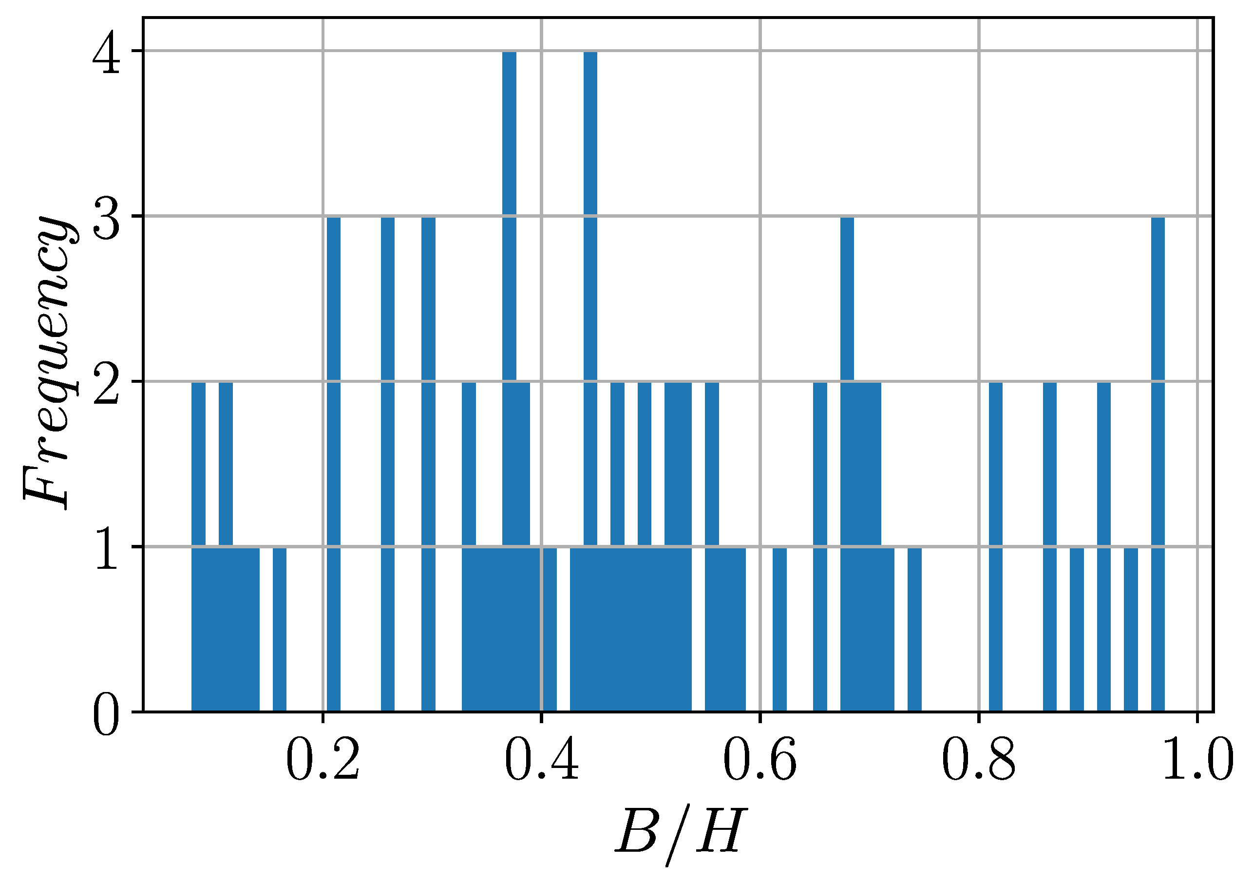
. The increased CO₂ emissions by higher strength concrete can be attributed to the greater amounts of CO₂ released in the production of higher strength concrete. For each concrete class, increased requirement for $N_{u,min}$ was accompanied by higher CO₂ emissions. The frequency distribution of the $B/H$ ratios obtained by using the social spider algorithm is shown in Figure 19. 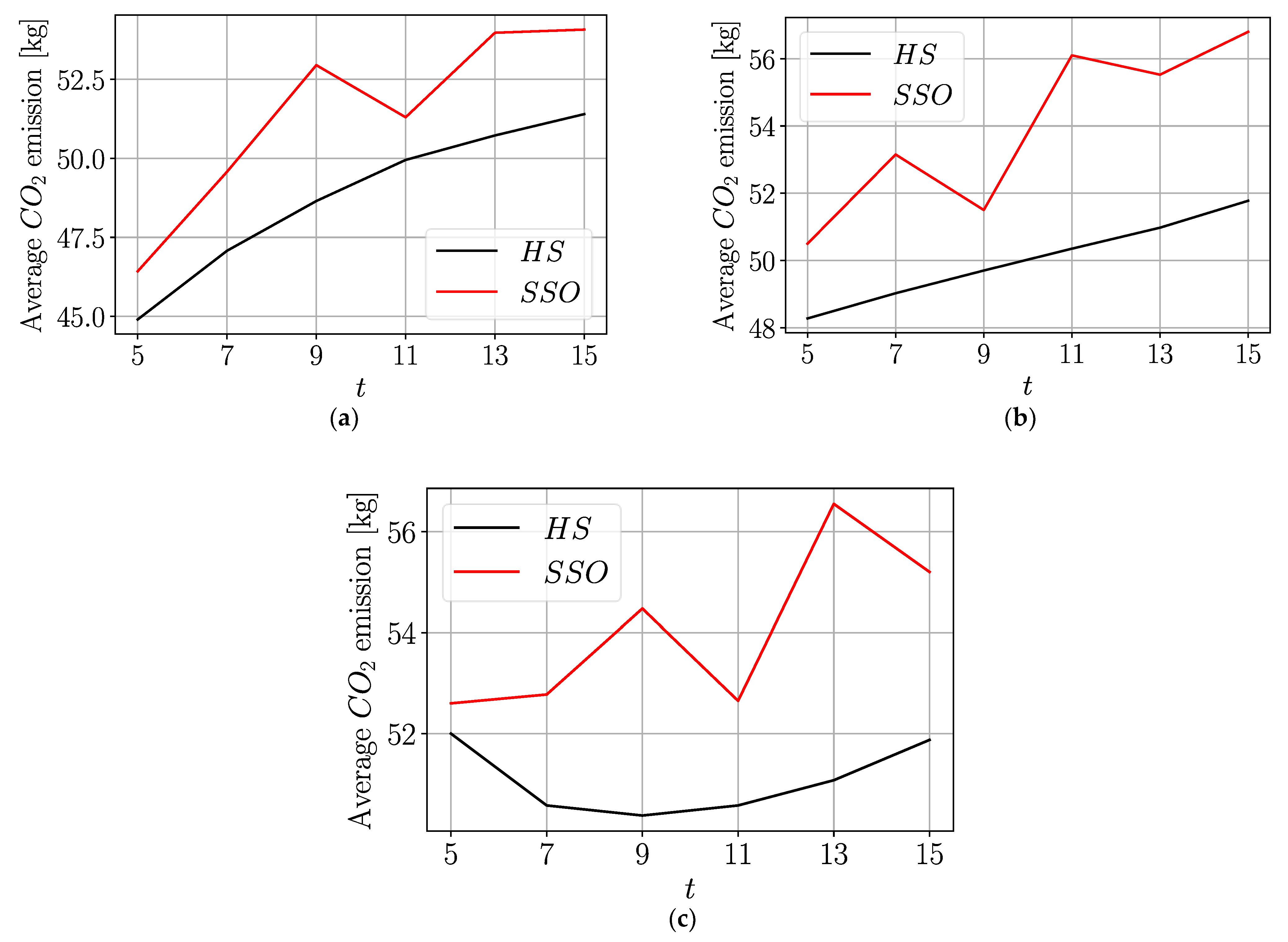Unlike the result of the harmony search optimization, no clustering of the $B/H$ ratios in a certain range of values could be observed. A comparison of the average CO₂ emissions achieved by using SSO and harmony search algorithms for a rectangular cross section can be observed in Figure 20 for the concrete classes C25, C40, and C60. The harmony search procedure delivered better-performing configurations for all wall thicknesses and concrete classes. The results obtained from the harmony search method were about 6.2% lower CO₂ emission than SSO for rectangular cross sections.

4. Discussion

The current study demonstrated the optimization results obtained by using the well-established harmony search algorithm and a newly developed metaheuristic technique called social spider optimization. The objective of the optimization was to reduce CO₂ emissions related to the production process of CFST stub columns with rectangular cross-section under concentric loading. The optimized cross-sectional dimensions have been tabulated for C25, C40, and C60 concrete classes. On average, the production related CO₂ emissions obtained by using the harmony search algorithm were 5.1, 7.8, and 5.4% lower than the CO₂ emissions obtained by using the social spider optimization. Both of these algorithms are non-gradient-based and evolutionary, while the social spider optimization starts with the assumptions that the natural development of social spider colonies would be a suitable fit for modeling various engineering systems. Although this assumption was warranted in the case of cross-section optimization of CFST columns, the performance of the technique is not necessarily superior to other evolutionary techniques such as the time-tested harmony search method. The performance of the harmony search algorithm can be significantly enhanced through parameter tuning, which is not the case for the social spider algorithm. The differences in the outcome of the two optimization techniques could also be attributed to the differences in the speed of convergence. As it is also demonstrated in the numerical examples of Appendix A and Appendix B, the social spider algorithm comes with a significantly higher complexity, which may have an adverse effect on the convergence speed and the number of iterations needed to converge to the global optima. As a result, after a given number of iterations, the algorithm with greater speed of convergence is expected to deliver better designs.

Further differences in the outcome of the two algorithms were observed in the $B/H$ values corresponding to the optimum designs. The frequency distributions of optimum $B/H$ for the two algorithms showed that the optimum $B/H$ values obtained through the social spider optimization do not exhibit a regular pattern as it was observed in the harmony search algorithm. The different results obtained through these methods can be attributed to the inherent randomness of both techniques. There are various randomly generated parameters built into both of these algorithms. Particularly, the social spider optimization has a larger number of these parameters attempting to mimic the random behaviors of spiders in nature, which could results in the differences in the distribution of the optimum $B/H$ ratios.

The focus of the current study was to minimize carbon emissions while keeping the compressive strength of the CFST stub columns above a certain level. On the other hand, a major priority of the design engineers is to assure the high strength of the structure. Due to the significance of using high strength materials, future studies in this field can include multi-objective optimization techniques having both CO₂ emissions and concrete compressive strengths as the objectives of optimization.

5. Conclusions

CFST members have been widely used in the field of structural engineering due to the enhanced mechanical properties that they provide. Due to increased awareness about the sustainability of construction and the carbon footprint associated with concrete, steel, and construction industries, there is an ongoing effort to reduce CO₂ emissions caused by the production of various construction materials. At the same time, it is responsible for structural engineers to design structures such as CFST columns in an optimum way so that they satisfy the load-carrying capacity requirements. Therefore, there is an increasing interest in the application of metaheuristic optimization techniques to structural optimization problems in recent years since these techniques have demonstrated that they are able to tackle many engineering problems more effectively. The social spider optimization algorithm is one of the newly developed metaheuristic techniques that can be effectively applied to design optimization problems. This study demonstrates a comparison between social spider optimization and harmony search algorithm applications for CFST columns. In terms of convergence speed and the quality of the optimization outcome, the harmony search algorithm was observed to be significantly superior compared to the social spider algorithm. The configurations obtained by using the harmony search algorithm resulted in a 6.2% lower CO₂ emissions on average. Furthermore, the speed of convergence of the harmony search method was observed to be an order of magnitude better than the social spider algorithm in most optimization cases. Moreover, it was observed that the configurations with greater concrete compressive strength also resulted in increased CO₂ emission. Furthermore, the results of the harmony search optimization showed clustering of the optimum $B/H$ ratios in a range from 0.6 to 0.75. Future research in this field can include CFST columns with various slenderness properties and column heights. In addition to the outer steel casing, another inner steel tube can be introduced. Moreover, the effect of using lightweight fiber-reinforced composite materials as casing can be investigated.