
Spatiotemporal Analysis of the Frost Regime in the Iberian Peninsula in the Context of Climate Change (1975–2018)

 , ,
, ,  ,
,
Abstract
:1. Introduction
2. Materials and Methods
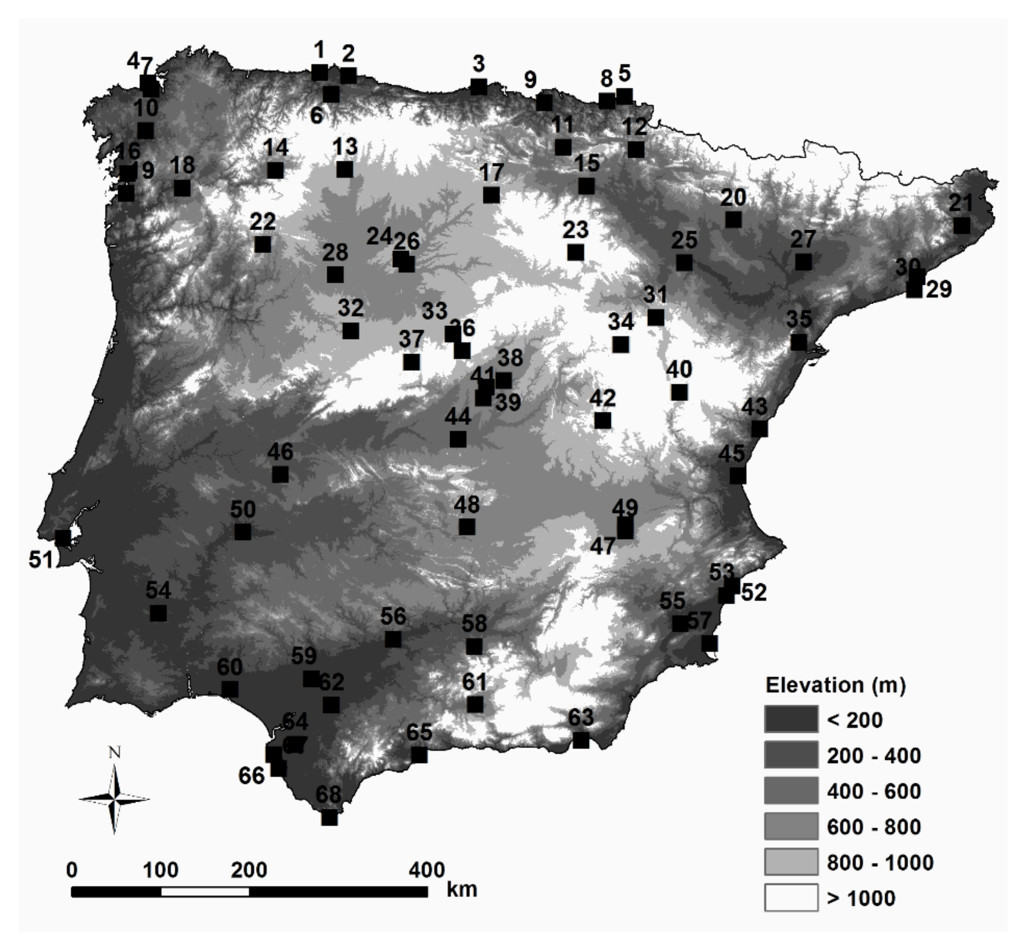
2.1. Study Area
2.2. Database and Interpolation Method
2.3. Frost Indices
2.3.1. Annual Frost Probability (%)
2.3.2. Frost Days (FD)
2.3.3. Mean Minimum Yearly Temperature (TMN)
2.3.4. First Frost Day (FFD)
2.3.5. Last Frost Day (LFD)
2.3.6. Frost-Free Period (FFP)
2.4. Trend Tests: Mann–Kendall Test (MK) and Sen’s Estimator
3. Results and Discussion
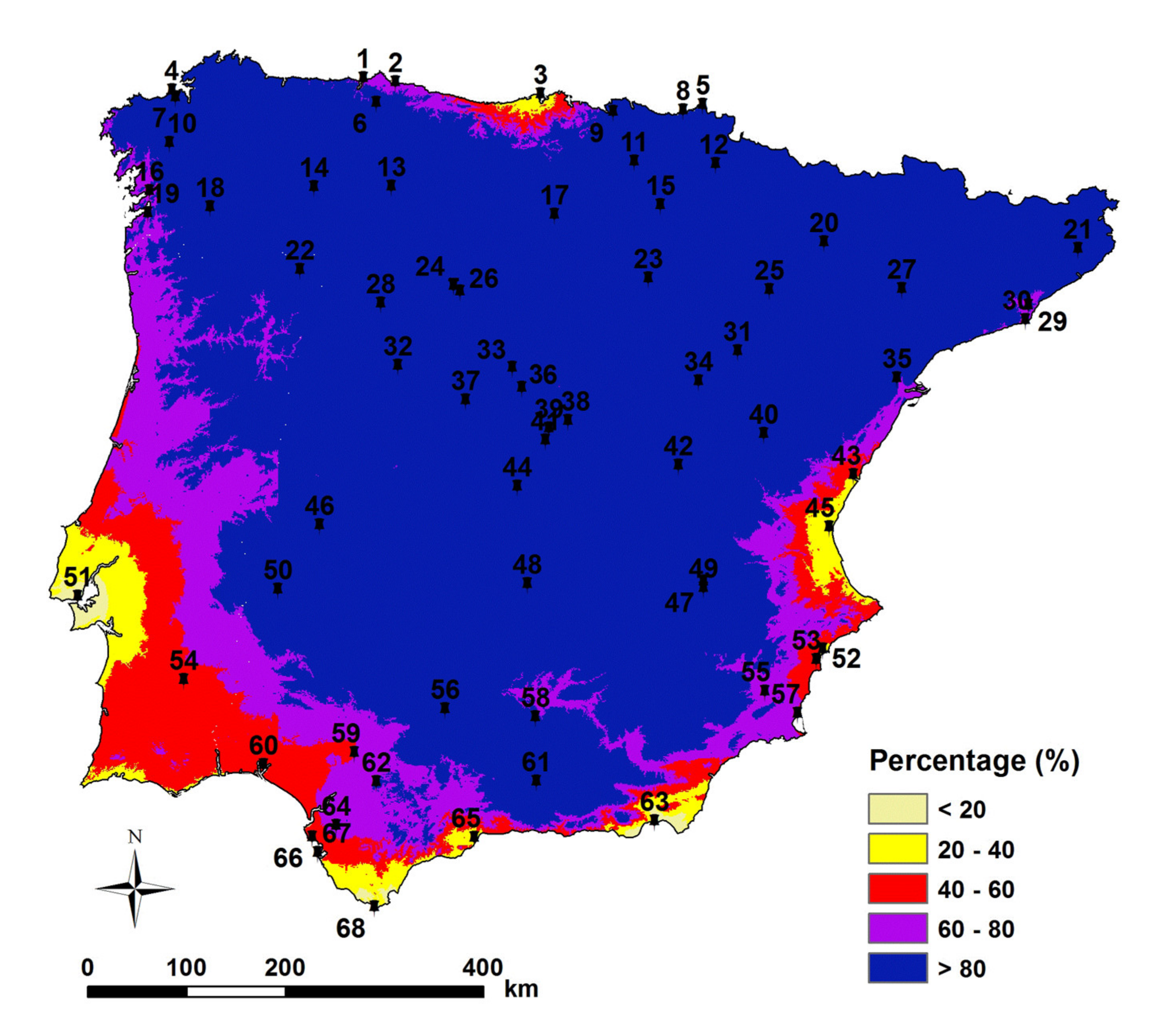
3.1. Probability of Frost
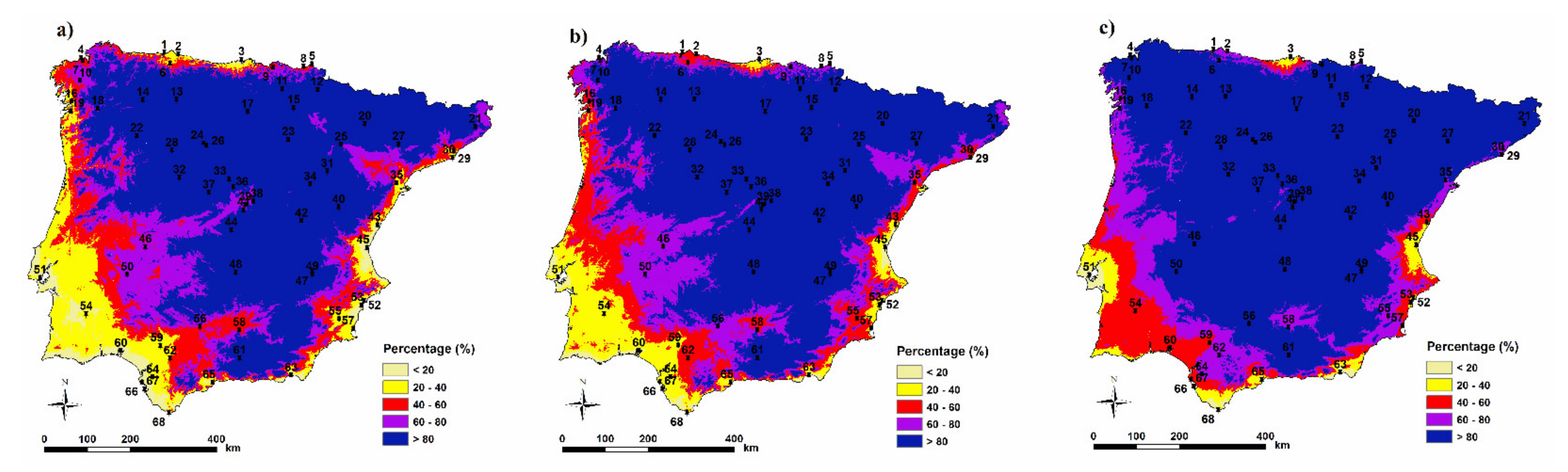
3.2. Probabilities of Light, Moderate, and Severe Frosts
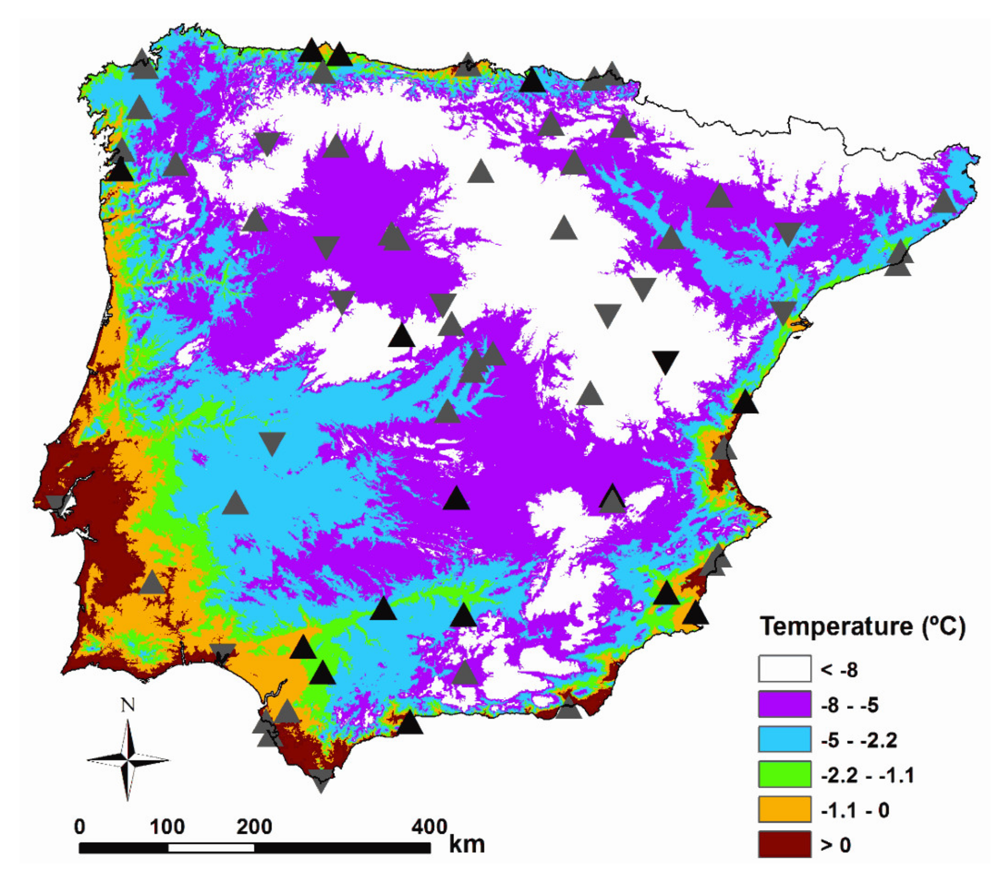
3.3. Mean Absolute Minimum Yearly Temperature
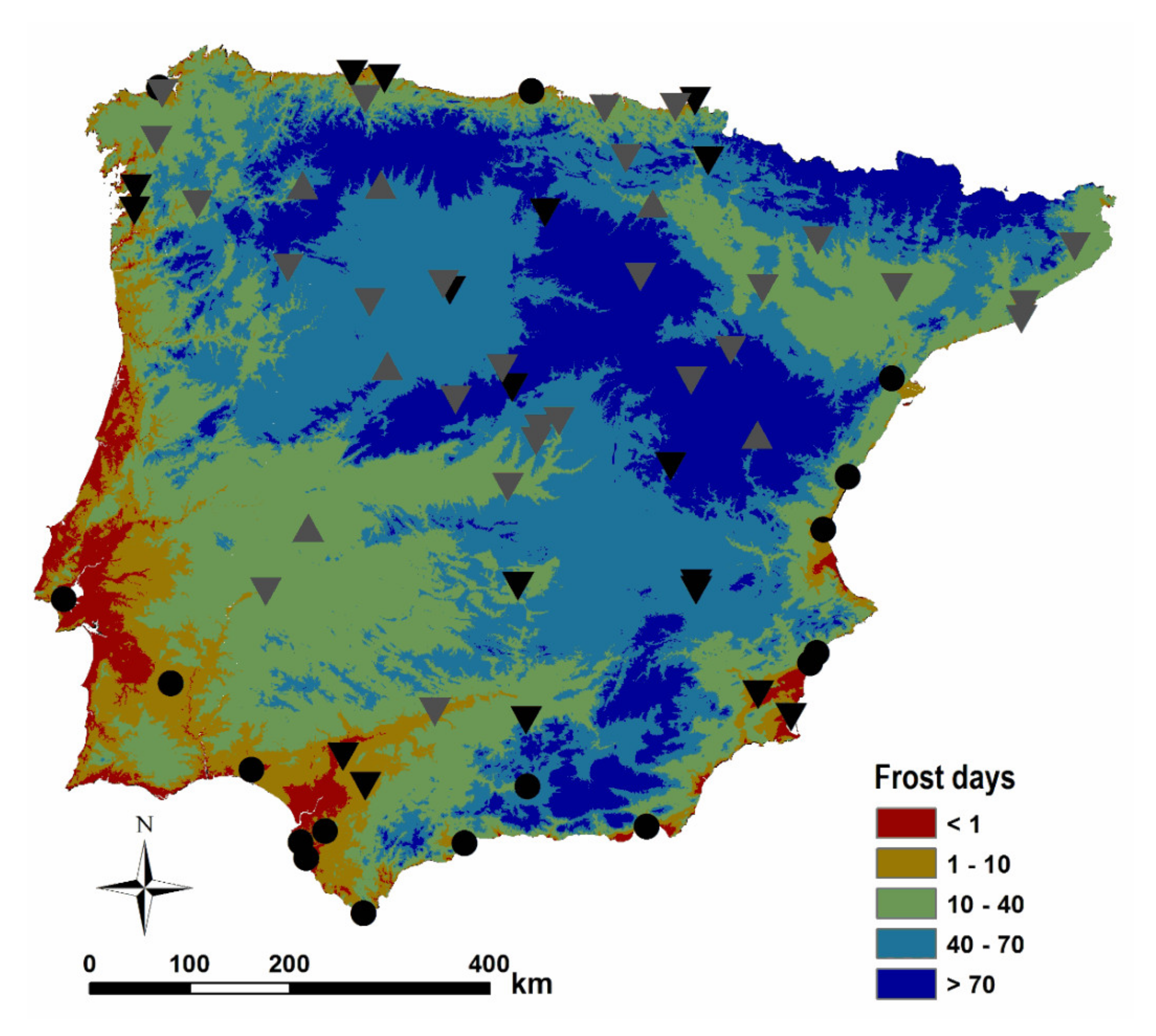
3.4. Frost Days
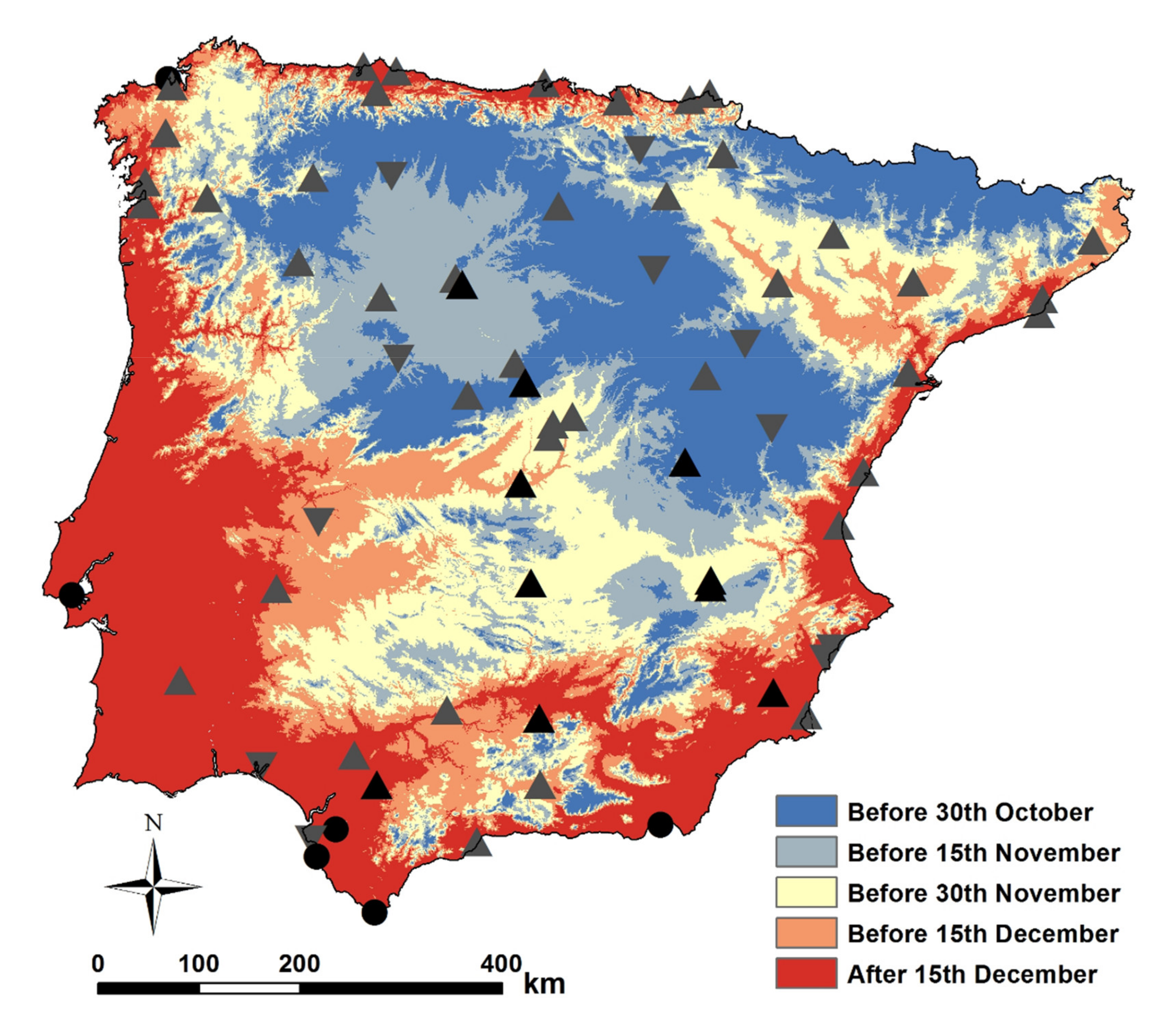
3.5. Date of the First Frost
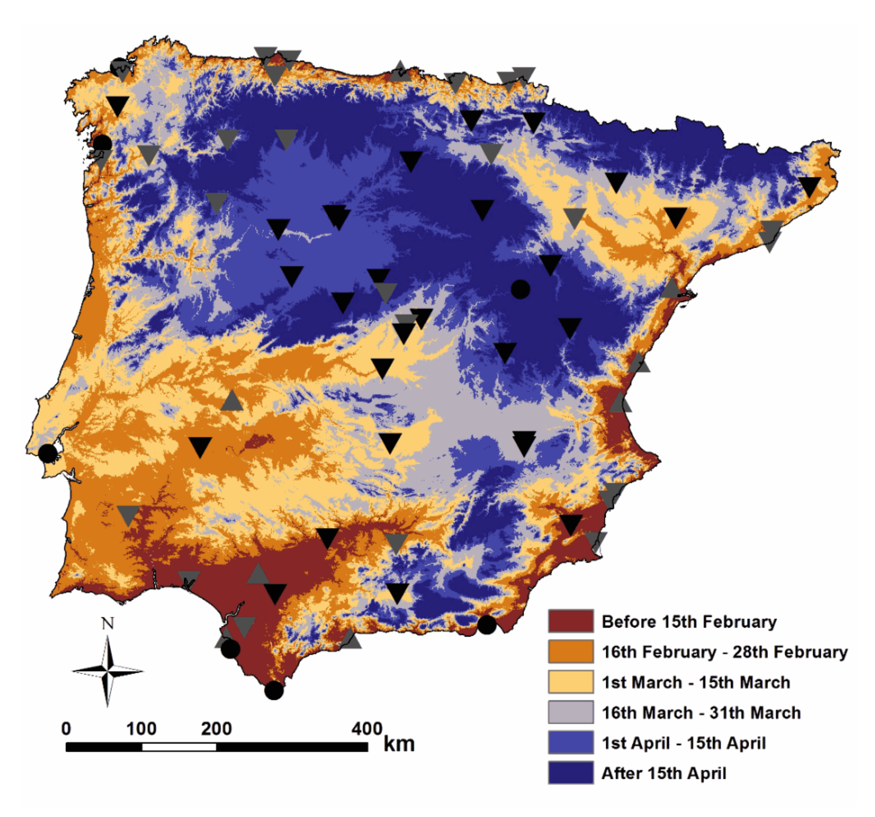
3.6. Date of the Last Frost
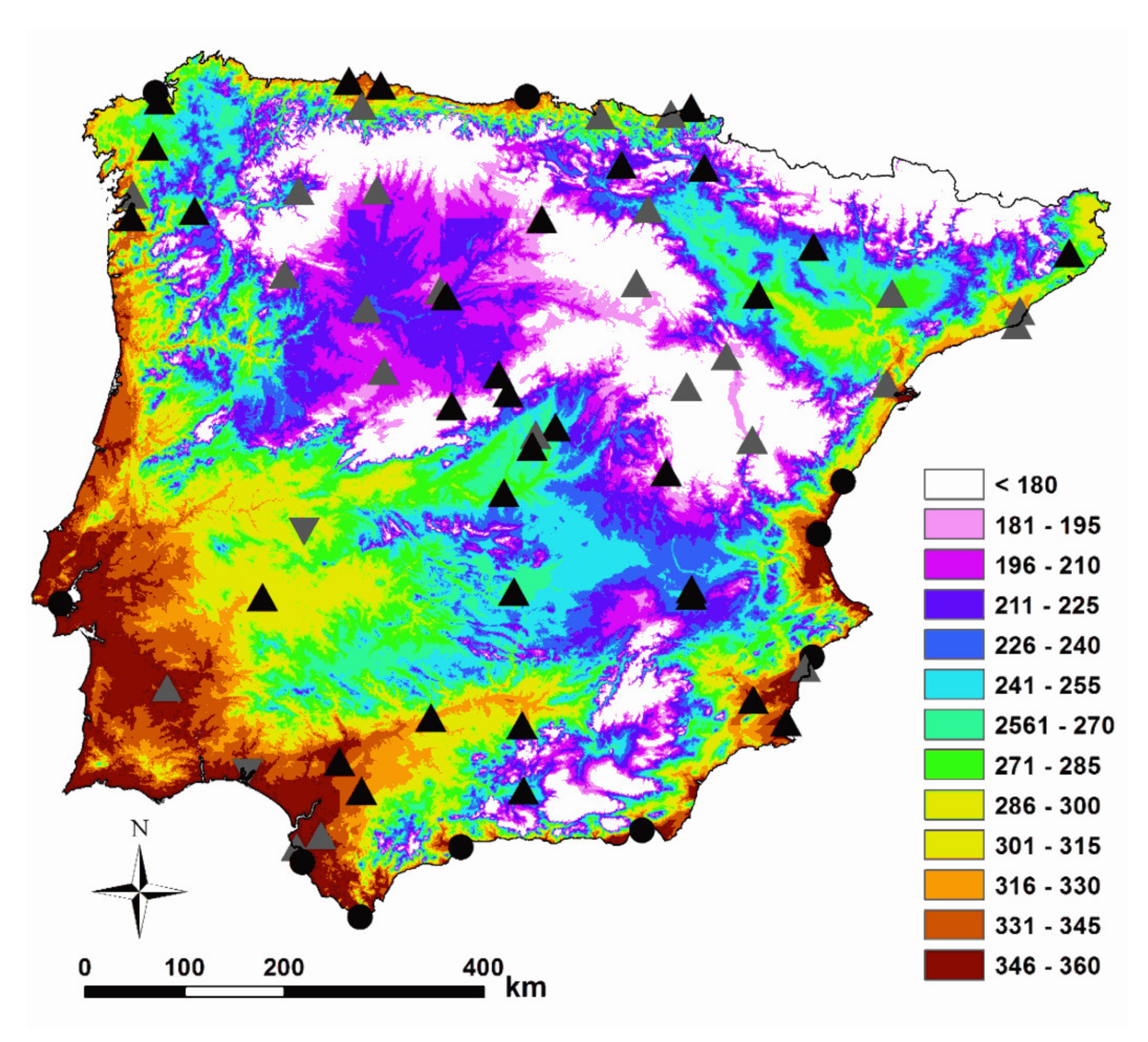
3.7. Frost-Free Period
4. Conclusions
Author Contributions
Funding
Institutional Review Board Statement
Informed Consent Statement
Data Availability Statement
Conflicts of Interest
References
- Parker, J. Cold resistance in woody plants. Bot. Rev. 1963, 29, 123–201. [Google Scholar] [CrossRef]
- Luo, Q. Temperature thresholds and crop production: A review. Clim. Chang. 2011, 109, 583–598. [Google Scholar] [CrossRef]
- Hatfield, J.L.; Prueger, J.H. Temperature extremes: Effect on plant growth and development. Weather Clim. Extrem. 2015, 10, 4–10. [Google Scholar] [CrossRef] [Green Version]
- Westwood, N.H. Fruticultura de Zonas Templadas; Mundi-Prensa: Madrid, Spain, 1982. [Google Scholar]
- Rodrigo, J. Spring frosts in deciduous fruit trees—Morphological damage and flower hardiness. Sci. Hortic. 2000, 85, 155–173. [Google Scholar] [CrossRef]
- Larcher, W. Effects of low temperature stress and frost injury on plant productivity. In Physiological Processes Limiting Plant Productivity; Johnson, C.B., Ed.; Butterworth: London, UK, 1981; pp. 253–269. [Google Scholar]
- Larcher, W.; Bauer, H. Ecological significance of resistance to low temperature. In Physiological Plant Ecology I: Responses to the Physical Environment; Lange, O.L., Nobel, P.S., Osmond, C.B., Ziegler, H., Eds.; Springer: Berlin/Heidelberg, Germany, 1981; pp. 403–437. [Google Scholar]
- Woodward, F.I.; Williams, B.G. Climate and plant distribution at global and local scales. Vegetatio 1987, 69, 189–197. [Google Scholar] [CrossRef]
- Lyons, J.M. Chilling injury in plants. Annu. Rev. Plant Physiol. 1973, 24, 445–466. [Google Scholar] [CrossRef]
- Pearce, R. Plant freezing and damage. Ann. Bot. 2001, 87, 417–424. [Google Scholar] [CrossRef]
- Snyder, R.L.; Melo-Abreu, J.D. Frost protection: Fundamentals, practice and economics. Frost Prot. Fundam. Pract. Econ. 2005, 1, 1–240. [Google Scholar]
- Rieger, M. Freeze protection for horticultural crops. Hort. Rev. 1989, 11, 45–109. [Google Scholar] [CrossRef]
- Augspurger, C.K. Spring 2007 warmth and frost: Phenology, damage and refoliation in a temperate deciduous forest. Funct. Ecol. 2009, 23, 1031–1039. [Google Scholar] [CrossRef]
- Gu, L.; Hanson, P.J.; Post, W.M.; Kaiser, D.P.; Yang, B.; Nemani, R.; Pallardy, S.G.; Meyers, T. The 2007 Eastern US spring freeze: Increased cold damage in a warming world? BioScience 2008, 58, 253–262. [Google Scholar] [CrossRef]
- Hufkens, K.; Friedl, M.A.; Keenan, T.F.; Sonnentag, O.; Bailey, A.; O’Keefe, J.; Richardson, A.D. Ecological impacts of a widespread frost event following early spring leaf-out. Glob. Chang. Biol. 2012, 18, 2365–2377. [Google Scholar] [CrossRef]
- Ningre, F.; Colin, F. Frost damage on the terminal shoot as a risk factor of fork incidence on common beech (Fagus sylvatica L.). Ann. For. Sci. 2007, 64, 79–86. [Google Scholar] [CrossRef] [Green Version]
- Kreyling, J.; Thiel, D.; Nagy, L.; Jentsch, A.; Huber, G.; Konnert, M.; Beierkuhnlein, C. Late frost sensitivity of juvenile Fagus sylvatica L. differs between Southern Germany and Bulgaria and depends on preceding air temperature. Eur. J. For. Res. 2012, 131, 717–725. [Google Scholar] [CrossRef]
- Vitasse, Y.; Schneider, L.; Rixen, C.; Christen, D.; Rebetez, M. Increase in the risk of exposure of forest and fruit trees to spring frosts at higher elevations in Switzerland over the last four decades. Agric. For. Meteorol. 2018, 248, 60–69. [Google Scholar] [CrossRef]
- Agroseguros 2018. Agrupación Española de Entidades Aseguradoras de los Seguros Agrarios Combinados S.A. Informe de Siniestralidades. 2018. Available online: https://agroseguro.es/fileadmin/propietario/Home/INFORMES_SINIESTRALIDAD/0._Informe_TOTAL_SINIESTRALIDADES_2018_30_septiembre_2018.pdf (accessed on 30 August 2019).
- Agroseguros 2019. Agrupación Española de Entidades Aseguradoras de los Seguros Agrarios Combinados S.A. Informe de Siniestralidades. 2019. Available online: https://agroseguro.es/fileadmin/propietario/Home/INFORMES_SINIESTRALIDAD/WEB_Informe_TOTAL_SINIESTRALIDADES_2019_31_agosto_2019.pdf (accessed on 30 August 2019).
- Raper, C.D.; Kramer, P.J. Soybeans: Improvement, production and uses. Stress Physiol. Agron. Monogr. 1987, 16, 589–641. [Google Scholar]
- Otegui, M.E.; Pereira, M.L. Fecha de siembra. In Producción de Granos; Bases funcionales para su manejo; Satorre, E.H., Arnold, R.L., Slafer, G.A., Fuente, E.B., Miralles, D.J., Otegui, M.E., Savin, R., Eds.; UBA: Buenos Aires, Argentina, 2003; pp. 259–275. [Google Scholar]
- Giannakopoulos, C.; Le Sager, P.; Bindi, M.; Moriondo, M.; Kostopoulou, E.; Goodess, C.M. Climatic changes and associated impacts in the mediterranean resulting from a 2 °C global warming. Glob. Planet. Chang. 2009, 68, 209–224. [Google Scholar] [CrossRef]
- Lionello, P.; Abrantes, F.; Gacic, M.; Planton, S.; Trigo, R.; Ulbrich, U. The climate of the Mediterranean region: Research progress and climate change impacts. Reg. Environ. Chang. 2014, 14, 1679–1684. [Google Scholar] [CrossRef]
- Kim, G.U.; Seo, K.H.; Chen, D. Climate change over the Mediterranean and current destruction of marine ecosystem. Sci. Rep. 2019, 9, 1–9. [Google Scholar] [CrossRef] [PubMed]
- Robeson, S.M. Increasing growing-season length in Illinois during the 20th century. Clim. Chang. 2002, 52, 219–238. [Google Scholar] [CrossRef]
- Fernández-Long, M.E.; Müller, G.V.; Beltrán-Przekurat, A.; Scarpati, O.E. Long-term and recent changes in temperature-based agroclimatic indices in Argentina. Int. J. Clim. 2013, 33, 1673–1686. [Google Scholar] [CrossRef]
- Yu, Q.; Li, L.; Luo, Q.; Eamus, D.; Xu, S.; Chen, C.; Wang, E.; Liu, J.; Nielsen, D.C. Year patterns of climate impact on wheat yields. Int. J. Clim. 2014, 34, 518–528. [Google Scholar] [CrossRef]
- Menzel, A.; Fabian, P. Growing season extended in Europe. Nature 1999, 397, 659. [Google Scholar] [CrossRef]
- Parmesan, C.; Yohe, G. A globally coherent fingerprint of climate change impacts across natural systems. Nature 2003, 421, 37–42. [Google Scholar] [CrossRef]
- Badeck, F.W.; Bondeau, A.; Böttcher, K.; Doktor, D.; Lucht, W.; Schaber, J.; Sitch, S. Responses of spring phenology to climate change. New Phytol. 2004, 162, 295–309. [Google Scholar] [CrossRef]
- Ge, Q.; Dai, J.; Cui, H.; Wang, H. Spatiotemporal variability in start and end of growing season in China related to climate variability. Remote Sens. 2016, 8, 433. [Google Scholar] [CrossRef] [Green Version]
- Cleland, E.; Chuine, I.; Menzel, A.; Mooney, H.; Schwartz, M. Shifting plant phenology in response to global change. Trends Ecol. Evol. 2007, 22, 357–365. [Google Scholar] [CrossRef]
- Menzel, A.; Sparks, T.H.; Estrella, N.; Koch, E.; Aasa, A.; Ahas, R.; Alm-Kübler, K.; Bissolli, P.; Braslavská, O.; Briede, A.; et al. European phenological response to climate change matches the warming pattern. Glob. Chang. Biol. 2006, 12, 1969–1976. [Google Scholar] [CrossRef]
- Han, H.; Bai, J.; Ma, G.; Yan, J. Vegetation phenological changes in multiple landforms and responses to climate change. ISPRS Int. J. Geo-Inf. 2020, 9, 111. [Google Scholar] [CrossRef] [Green Version]
- Liu, Q.; Piao, S.; Janssens, I.A.; Fu, Y.; Peng, S.; Lian, X.; Ciais, P.; Myneni, R.B.; Peñuelas, J.; Wang, T. Extension of the growing season increases vegetation exposure to frost. Nat. Commun. 2018, 9, 426. [Google Scholar] [CrossRef] [Green Version]
- Matiu, M.; Ankerst, D.P.; Menzel, A. Asymmetric trends in seasonal temperature variability in instrumental records from ten stations in Switzerland, Germany and the UK from 1864 to 2012. Int. J. Clim. 2016, 36, 13–27. [Google Scholar] [CrossRef] [Green Version]
- Easterling, D.R.; Evans, J.L.; Groisman, P.Y.; Karl, T.R.; Kunkel, K.E.; Ambenje, P. Observed variability and trends in extreme climate events: A brief review. Bull. Am. Meteorol. Soc. 2000, 81, 417–425. [Google Scholar] [CrossRef] [Green Version]
- Bootsma, A. Estimating minimum temperature and climatological freeze risk in hilly terrain. Agric. Meteorol. 1976, 16, 425–443. [Google Scholar] [CrossRef]
- Laughlin, G.P.; Kalma, J.D. Frost hazard assessment from local weather and terrain data. Agric. For. Meteorol. 1987, 40, 1–16. [Google Scholar] [CrossRef]
- Crimp, S.J.; Gobbett, D.; Kokic, P.; Nidumolu, U.; Howden, M.; Nicholls, N. Recent seasonal and long-term changes in southern Australian frost occurrence. Clim. Chang. 2016, 139, 115–128. [Google Scholar] [CrossRef]
- Hosseini, S.M.; Karbalaee, A.; Hosseini, S.A. Spatiotemporal changes of early fall and late spring frost and its trend based an daily minimum temperature in Iran. Arab. J. Geosci. 2021, 14, 304. [Google Scholar] [CrossRef]
- Gobbett, D.; Nidumolu, U.; Crimp, S. Modelling frost generates insights for managing risk of minimum temperature extremes. Weather Clim. Extrem. 2020, 27, 100176. [Google Scholar] [CrossRef]
- Gobbett, D.; Nidumolu, U.; Jin, H.; Hayman, P.; Gallant, J. Minimum temperature mapping augments Australian grain farmers’ knowledge of frost. Agric. For. Meteorol. 2021, 304, 108422. [Google Scholar] [CrossRef]
- Srivastava, P.K.; Pandey, P.C.; Kumar, P.; Raghubanshi, A.S.; Han, D. Geospatial Technology for Water Resource Applications; CRC Press: Boca Raton, FL, USA, 2016. [Google Scholar]
- Beck, H.; Zimmermann, N.; McVicar, T.; Vergopolan, N.; Berg, A.; Wood, E.F. Present and future Köppen-Geiger climate classification maps at 1-km resolution. Sci. Data 2018, 5, 180214. [Google Scholar] [CrossRef] [Green Version]
- AEMET. Iberian Climate Atlas: Air Temperature and Precipitation (1971e2000); Ministerio de MedioAmbiente, Medio Rural y Marino: Madrid, Spain, 2011. [Google Scholar]
- ECA&D Algorithm Basis Document (ATBD); Royal Netherlands Meteorological Institute KNMI: De Bilt, The Netherlands, 2013.
- Klein-Tank, A.M.; Wijngaard, J.B.; Können, G.P.; Böhm, R.; Demarée, G.; Gocheva, A.; Mileta, M.; Pashiardis, S.; Hejkrlik, L.; Kern-Hansen, C.; et al. Daily dataset of 20th-century surface air temperature and precipitation series for the European climate assessment. Int. J. Clim. 2002, 22, 1441–1453. [Google Scholar] [CrossRef]
- Haylock, M.R.; Hofstra, N.; Klein-Tank, A.M.; Klok, E.J.; Jones, P.D.; New, M. A European daily high-resolution gridded data set of surface temperature and precipitation for 1950–2006. J. Geophys. Res. Atmos. 2008, 113. [Google Scholar] [CrossRef] [Green Version]
- Wijngaard, J.B.; Klein Tank, A.M.; Können, G.P. Homogeneity of 20th century European daily temperature and precipitation series. Int. J. Clim. 2003, 23, 679–692. [Google Scholar] [CrossRef]
- WMO Guide to Climatological Practices, No. 100; World Meteorological Organization: Geneva, Switzerland, 2011.
- Allen, R.G.; Pereira, L.S.; Raes, D.; Smith, M. Crop evapotranspiration. In Guidelines for Computing Crop Water Requirements; FAO irrigation and drainage paper, No. 56; FAO: Rome, Italy, 1998. [Google Scholar]
- Goovaerts, P. Using elevation to aid the geostatistical mapping of rainfall erosivity. Catena 1999, 34, 227–242. [Google Scholar] [CrossRef]
- Hornstein, R.A. Freezing Temperature Probabilities at Experimental Farms in the Maritime Provinces; Meteorol. Branch Circ. 3411, Tec. 337; Canada Department Transport: Toronto, ON, Canada, 1960. [Google Scholar]
- Ouellet, C.E. Préparation et usage des tables de probabilité de gelée. Agriculture 1962, 19, 105–111. [Google Scholar]
- WMO. Protection against Frost Damage; No. 100, TP. 60; WMO, World Meteorological Organization: Geneva, Switzerland, 1963. [Google Scholar]
- Mann, H.B. Nonparametric tests against trend. Econometrica 1945, 13, 245–259. [Google Scholar] [CrossRef]
- Kendall, M.G. Rank Correlation Methods; Charles Griffin: London, UK, 1975. [Google Scholar]
- WMO. Volume II—Management of water resources and application of hydrological practices. In Guide to Hydrological Practices; WMO-No. 168; World Meteorological Organization: Geneva, Switzerland, 2009. [Google Scholar]
- Sen, P.K. Estimates of the regression coefficient based on Kendall’s Tau. J. Am. Stat. Assoc. 1968, 63, 1379–1389. [Google Scholar] [CrossRef]
- Salmi, T.; Mäattä, A.; Anttila, P.; Ruoho-Airola, T.; Amnell, T. Detecting Trends of Annual Values of Atmospheric Pollutants by the Mann-Kendall Test and Sen’s Slope Estimates–the Excel Template Application MAKESENS; Publication on Air Quality, Finnish Meteorological Institute: Helsinki, Finland, 2002. [Google Scholar]
- Moeletsi, M.; Tongwane, M. Spatiotemporal Variation of Frost within Growing Periods. Adv. Meteorol. 2017, 2017, 5472869. [Google Scholar] [CrossRef] [Green Version]
- Núñez, L.M.; Moreno, J.V.; Chazarra, A.; Abaroa, T.G.; Avello, E.; Botey, M.R. Mapas de Riesgo: Heladas y Horas de Frío en la España Peninsular (Periodo 2002–2012); Ministerio de Agricultura, Alimentación y Medio Ambiente, Ed.; Agencia Estatal de Meteorología: Madrid, Spain, 2015. [Google Scholar]
- Fridley, J.D. Downscaling climate over complex terrain: High finescale (<1000 m) spatial variation of near-ground temperatures in a montane forested landscape (Great Smoky Mountains). J. Appl. Meteorol. Climatol. 2009, 48, 1033–1049. [Google Scholar] [CrossRef] [Green Version]
- Pouteau, R.; Rambal, S.; Ratte, J.P.; Gogé, F.; Joffre, R.; Winkel, T. Downscaling MODIS-derived maps using GIS and boosted regression trees: The case of frost occurrence over the arid Andean highlands of Bolivia. Remote Sens. Environ. 2011, 115, 117–129. [Google Scholar] [CrossRef] [Green Version]
- Neuner, G.; Hacker, J. Ice Formation and propagation in alpine plants. In Plants in Alpine Regions: Cell Physiology of Adaption and Survival Strategies; Lütz, C., Ed.; Springer: Vienna, Austria, 2012; pp. 163–174. [Google Scholar]
- Neuner, G. Frost resistance in alpine woody plants. Front. Plant Sci. 2014, 5, 654. [Google Scholar] [CrossRef] [Green Version]
- Abanades, J.C.; Prats, J.C.; de Lucas, M.C.; García, F.F.; Zulaica, C.G.; De Marcos, L.G. El Cambio Climático en España. Estado de Situación; Documento Resumen; Instituto para la Diversificación y el Ahorro de Energía (IDEA), Oficina Española de Cambio Climático (OECC): Madrid, Spain, 2007. [Google Scholar]
- De Lima, M.I.; Santo, F.E.; Ramos, A.M.; de Lima, J.L. Recent changes in daily precipitation and surface air temperature extremes in mainland Portugal, in the period 1941–2007. Atmos. Res. 2013, 127, 195–209. [Google Scholar] [CrossRef]
- Zeinali, B.; Teymouri, M.; Asghari, S.; Mohammadi, M.; Gupta, V. A study of frost occurrence and minimum temperatures in Iran. J. Earth Syst. Sci. 2019, 128, 134. [Google Scholar] [CrossRef] [Green Version]
- Karl, T.R.; Knight, R.W.; Gallo, K.P.; Peterson, T.C.; Jones, P.D.; Kukla, G.; Plummer, N.; Razuvayev, V.; Lindseay, J.; Charlson, R.J. A new perspective on recent global warming: Asymmetric trends of daily maximum and minimum temperature. Bull. Am. Meteorol. Soc. 1993, 74, 1007–1023. [Google Scholar] [CrossRef] [Green Version]
- Menzel, A.; Jakobi, G.; Ahas, R.; Scheifinger, H.; Estrella, N. Variations of the climatological growing season (1951–2000) in Germany compared with other countries. Int. J. Clim. 2003, 23, 793–812. [Google Scholar] [CrossRef]
- Fernández-Montes, S.; Rodrigo, F.S. Trends in seasonal indices of daily temperature extremes in the Iberian Peninsula, 1929–2005. Int. J. Clim. 2012, 32, 2320–2332. [Google Scholar] [CrossRef]
- Dai, J.; Wang, H.; Ge, Q. The decreasing spring frost risks during the flowering period for woody plants in temperate area of eastern China over past 50 years. J. Geogr. Sci. 2013, 23, 641–652. [Google Scholar] [CrossRef]
- Pi, Y.; Yu, Y.; Zhang, Y.; Xu, C.; Yu, R. Extreme Temperature Events during 1960–2017 in the Arid Region of Northwest China: Spatiotemporal Dynamics and Associated Large-Scale Atmospheric Circulation. Sustainability 2020, 12, 1198. [Google Scholar] [CrossRef] [Green Version]
- Piticar, A. Changes in agro-climatic indices related to temperature in Central Chile. Int. J. Biometeorol. 2019, 63, 499–510. [Google Scholar] [CrossRef] [PubMed]
- Christensen, J.H.; Christensen, O.B. A summary of the PRUDENCE model projections of changes in European climate by the end of this century. Clim. Chang. 2007, 81, 7–30. [Google Scholar] [CrossRef]
- IPCC 2013 Climate Change; The Physical Science Basis; IPCC: Geneva, Switzerland, 2013.
- Moonen, A.C.; Ercoli, L.; Mariotti, M.; Masoni, A. Climate change in Italy indicated by agrometeorological indices over 122 years. Agric. For. Meteorol. 2002, 111, 13–27. [Google Scholar] [CrossRef]
- Moeletsi, M.E.; Tongwane, M.; Tsubo, M. The study of frost occurrence in Free State Province of South Africa. Adv. Meteorol. 2016, 2016, 9586150. [Google Scholar] [CrossRef] [Green Version]
- Tait, A.; Zheng, X. Mapping frost occurrence using satellite data. J. Appl. Meteorol. 2003, 42, 193–203. [Google Scholar] [CrossRef]
- Rahimi, M.; Hajjam, S.; Khalili, A.; Kamali, G.A.; Stigter, C.J. Risk analysis of first and last frost occurrences in the Central Alborz region, Iran. Int. J. Clim. 2007, 27, 349–356. [Google Scholar] [CrossRef]
- Varshavian, V.; Ghahreman, N.; Khalili, A.; Hajjam, S. Statistical analysis of first and last frost occurrences and length of frost free period during the past decades in different regions of Iran. Environ. Inform. Arch. 2007, 5, 631–637. [Google Scholar]
- Scheifinger, H.; Menzel, A.; Koch, E.; Peter, C. Trends of spring time frost events and phenological dates in Central Europe. Theor. Appl. Clim. 2003, 74, 41–51. [Google Scholar] [CrossRef]
- Potop, V.; Zahraniček, P.; Türkott, L.; Štěpánek, P.; Soukup, J. Risk occurrences of damaging frosts during the growing season of vegetables in the Elbe river lowland, the Czech Republic. Nat. Hazards 2013, 71, 1–19. [Google Scholar] [CrossRef]
- Genovese, G.; Bettio, M.; Orlandi, S.; Boogaard, H.L.; Petrakos, M.; Stavropoulos, P.; Glossioti, M. Methodology of the MARS crop yield forecasting system. Stat. Data Collect. Process. Anal. 2004, 4, 21291. [Google Scholar]
- Piao, S.; Friedlingstein, P.; Ciais, P.; Viovy, N.; Demarty, J. Growing season extension and its impact on terrestrial carbon cycle in the Northern Hemisphere over the past 2 decades. Glob. Biogeochem. Cycles 2007, 21, GB3018. [Google Scholar] [CrossRef]
- Keenan, T.F.; Gray, J.; Friedl, M.A.; Toomey, M.; Bohrer, G.; Hollinger, D.Y.; Munger, J.W.; O’Keefe, J.; Schmid, H.P.; Wing, I.S.; et al. Net carbon uptake has increased through warming-induced changes in temperate forest phenology. Nat. Clim. Chang. 2014, 4, 598–604. [Google Scholar] [CrossRef]
- Geiger, R.; Aron, R.H.; Todhunter, P. The microclimate of caves. In The Climate near the Ground; Rowman and Littlefield Publishers Inc.: Lanham, MD, USA, 2003; pp. 418–424. [Google Scholar]


| Elevation | Latitude | Longitude | Elevation | Latitude | Longitude | ||||
|---|---|---|---|---|---|---|---|---|---|
| No | Station | (m) | (°N) | (+°E, −°W) | No | Station | (m) | (°N) | (+°E, −°W) |
| 1 | Avilés | 127 | 43.57 | −6.04 | 35 | Tortosa | 44 | 40.82 | 0.49 |
| 2 | Gijón | 3 | 43.54 | −5.64 | 36 | Navacerrada | 1894 | 40.78 | −4.01 |
| 3 | Santander | 64 | 43.46 | −3.82 | 37 | Ávila | 1130 | 40.66 | −4.68 |
| 4 | Coruña | 58 | 43.37 | −8.42 | 38 | Torrejón | 611 | 40.48 | −3.45 |
| 5 | Fuenterrabía | 4 | 43.36 | −1.79 | 39 | Madrid | 667 | 40.41 | −3.68 |
| 6 | Oviedo | 336 | 43.35 | −5.87 | 40 | Teruel | 900 | 40.35 | −1.12 |
| 7 | Alvedro | 98 | 43.31 | −8.37 | 41 | Getafe | 617 | 40.30 | −3.72 |
| 8 | Igueldo | 251 | 43.31 | −2.04 | 42 | Cuenca | 945 | 40.07 | −2.14 |
| 9 | Bilbao | 42 | 43.30 | −2.91 | 43 | Castellón | 35 | 39.95 | −0.07 |
| 10 | Santiago de Compostela | 370 | 42.89 | −8.41 | 44 | Toledo | 515 | 39.88 | −4.05 |
| 11 | Vitoria | 521 | 42.85 | −2.65 | 45 | Cáceres | 459 | 39.48 | −6.37 |
| 12 | Pamplona | 442 | 42.82 | −1.64 | 46 | Valencia | 11 | 39.48 | −0.37 |
| 13 | León | 916 | 42.59 | −5.65 | 47 | Albacete | 674 | 39.01 | −1.86 |
| 14 | Ponferrada | 534 | 42.56 | −6.6 | 48 | Ciudad Real | 628 | 38.99 | −3.92 |
| 15 | Agoncillo | 353 | 42.45 | −2.33 | 49 | Los Llanos | 704 | 38.95 | −1.86 |
| 16 | Pontevedra | 108 | 42.44 | −8.62 | 50 | Talavera la Real | 185 | 38.88 | −6.83 |
| 17 | Villafría | 890 | 42.36 | −3.63 | 51 | Lisboa | 77 | 38.72 | −9.15 |
| 18 | Ourense | 143 | 42.33 | −7.86 | 52 | Alicante | 81 | 38.37 | −0.49 |
| 19 | Vigo | 261 | 42.24 | −8.62 | 53 | Alicante | 43 | 38.28 | −0.57 |
| 20 | Huesca | 541 | 42.08 | −0.33 | 54 | Beja | 246 | 38.02 | −7.87 |
| 21 | Girona | 143 | 41.91 | 2.76 | 55 | Murcia | 61 | 38.00 | −1.17 |
| 22 | Braganza | 690 | 41.80 | −6.73 | 56 | Córdoba | 90 | 37.84 | −4.85 |
| 23 | Soria | 1082 | 41.78 | −2.48 | 57 | San Javier | 4 | 37.79 | −0.8 |
| 24 | Villanubla | 846 | 41.70 | −4.85 | 58 | Jaén | 582 | 37.78 | −3.81 |
| 25 | Zaragoza | 247 | 41.66 | −1.01 | 59 | Sevilla | 34 | 37.42 | −5.88 |
| 26 | Valladolid | 735 | 41.65 | −4.77 | 60 | Huelva | 19 | 37.28 | −6.91 |
| 27 | Lleida | 192 | 41.63 | 0.60 | 61 | Granada | 567 | 37.19 | −3.79 |
| 28 | Zamora | 656 | 41.52 | −5.73 | 62 | Morón de la Frontera | 87 | 37.16 | −5.62 |
| 29 | Barcelona | 412 | 41.42 | 2.12 | 63 | Almería | 7 | 36.83 | −2.45 |
| 30 | Barcelona | 4 | 41.29 | 2.07 | 64 | Jerez de la Frontera | 27 | 36.75 | −6.06 |
| 31 | Daroca | 779 | 41.11 | −1.41 | 65 | Málaga | 7 | 36.67 | −4.49 |
| 32 | Salamanca | 790 | 40.96 | −5.50 | 66 | Rota | 21 | 36.64 | −6.33 |
| 33 | Segovia | 1005 | 40.95 | −4.13 | 67 | Cádiz | 1 | 36.50 | −6.26 |
| 34 | Molina de Aragón | 1056 | 40.84 | −1.89 | 68 | Tarifa | 32 | 36.02 | −5.6 |
| No | Station | FP | LP | MF | SF | No | Station | FP | LP | MF | SF |
|---|---|---|---|---|---|---|---|---|---|---|---|
| % | % | % | % | % | % | % | % | ||||
| 1 | Avilés | 75.6 | 73.2 | 36.6 | 12.2 | 35 | Tortosa | 82.9 | 78.0 | 39.0 | 14.6 |
| 2 | Gijón | 68.3 | 68.3 | 41.5 | 22.0 | 36 | Navacerrada | 100.0 | 100.0 | 100.0 | 100.0 |
| 3 | Santander | 19.5 | 19.5 | 2.4 | 0.0 | 37 | Ávila | 100.0 | 100.0 | 100.0 | 100.0 |
| 4 | Coruña | 4.9 | 4.9 | 0.0 | 0.0 | 38 | Torrejón | 100.0 | 100.0 | 100.0 | 100.0 |
| 5 | Fuenterrabía | 97.6 | 97.6 | 87.8 | 75.6 | 39 | Madrid | 97.6 | 97.6 | 87.8 | 61.0 |
| 6 | Oviedo | 92.7 | 87.8 | 70.7 | 51.2 | 40 | Teruel | 100.0 | 100.0 | 100.0 | 100.0 |
| 7 | Alvedro | 97.6 | 97.6 | 80.5 | 56.1 | 41 | Getafe | 100.0 | 100.0 | 97.6 | 95.1 |
| 8 | Igueldo | 90.2 | 82.9 | 68.3 | 53.7 | 42 | Cuenca | 100.0 | 100.0 | 100.0 | 100.0 |
| 9 | Bilbao | 97.6 | 97.6 | 75.6 | 68.3 | 43 | Castellón | 39.0 | 39.0 | 17.1 | 4.9 |
| 10 | Santiago | 100.0 | 100.0 | 95.1 | 75.6 | 44 | Toledo | 100.0 | 97.6 | 100.0 | 100.0 |
| 11 | Vitoria | 100.0 | 100.0 | 100.0 | 100.0 | 45 | Cáceres | 90.2 | 90.2 | 70.7 | 61.0 |
| 12 | Pamplona | 100.0 | 100.0 | 100.0 | 100.0 | 46 | Valencia | 22.0 | 19.5 | 7.3 | 2.4 |
| 13 | León | 100.0 | 100.0 | 100.0 | 100.0 | 47 | Albacete | 100.0 | 100.0 | 100.0 | 97.6 |
| 14 | Ponferrada | 100.0 | 100.0 | 97.6 | 100.0 | 48 | Ciudad Real | 100.0 | 100.0 | 100.0 | 95.1 |
| 15 | Agoncillo | 100.0 | 100.0 | 100.0 | 95.1 | 49 | Los Llanos | 100.0 | 100.0 | 100.0 | 100.0 |
| 16 | Pontevedra | 65.9 | 61.0 | 39.0 | 9.8 | 50 | Talavera la Real | 97.6 | 95.1 | 92.7 | 82.9 |
| 17 | Villafría | 100.0 | 100.0 | 100.0 | 100.0 | 51 | Lisboa | 2.4 | 0.0 | 0.0 | 2.4 |
| 18 | Ourense | 97.6 | 97.6 | 90.2 | 90.2 | 52 | Alicante | 36.6 | 34.1 | 17.1 | 2.4 |
| 19 | Vigo | 80.5 | 78.0 | 31.7 | 12.2 | 53 | Alicante | 43.9 | 36.6 | 22.0 | 4.9 |
| 20 | Huesca | 100.0 | 100.0 | 97.6 | 97.6 | 54 | Beja | 57.1 | 52.4 | 31.0 | 19.0 |
| 21 | Girona | 100.0 | 100.0 | 100.0 | 100.0 | 55 | Murcia | 82.9 | 78.0 | 63.4 | 39.0 |
| 22 | Braganza | 100.0 | 100.0 | 100.0 | 100.0 | 56 | Córdoba | 92.5 | 90.0 | 65.0 | 57.5 |
| 23 | Soria | 100.0 | 100.0 | 100.0 | 100.0 | 57 | San Javier | 78.0 | 65.9 | 29.3 | 14.6 |
| 24 | Villanubla | 100.0 | 100.0 | 100.0 | 100.0 | 58 | Jaén | 85.0 | 80.0 | 55.0 | 47.5 |
| 25 | Zaragoza | 100.0 | 100.0 | 95.1 | 90.2 | 59 | Sevilla | 56.1 | 56.1 | 29.3 | 19.5 |
| 26 | Valladolid | 100.0 | 100.0 | 100.0 | 100.0 | 60 | Huelva | 46.3 | 46.3 | 12.2 | 4.9 |
| 27 | Lleida | 100.0 | 100.0 | 100.0 | 100.0 | 61 | Granada | 100.0 | 100.0 | 97.6 | 97.6 |
| 28 | Zamora | 100.0 | 100.0 | 100.0 | 97.6 | 62 | Morón de la Frontera | 85.4 | 80.5 | 65.9 | 51.2 |
| 29 | Barcelona | 78.0 | 78.0 | 41.5 | 34.1 | 63 | Almería | 2.4 | 0.0 | 0.0 | 2.4 |
| 30 | Barcelona | 78.0 | 73.2 | 56.1 | 19.5 | 64 | Jerez de la Frontera | 73.2 | 68.3 | 36.6 | 31.7 |
| 31 | Daroca | 100.0 | 100.0 | 100.0 | 100.0 | 65 | Málaga | 19.5 | 14.6 | 7.3 | 2.4 |
| 32 | Salamanca | 100.0 | 100.0 | 100.0 | 100.0 | 66 | Rota | 43.9 | 39.0 | 22.0 | 9.8 |
| 33 | Segovia | 100.0 | 100.0 | 100.0 | 97.6 | 67 | Cádiz | 4.9 | 2.4 | 4.9 | 2.4 |
| 34 | Molina de Aragón | 100.0 | 100.0 | 100.0 | 100.0 | 68 | Tarifa | 2.4 | 0.0 | 0.0 | 2.4 |
| TN | FD | TN | FD | ||||||||||||||||
|---|---|---|---|---|---|---|---|---|---|---|---|---|---|---|---|---|---|---|---|
| No | Station | Mean | SD | Q | Mean | SD | Q | N° | Station | Mean | SD | Q | Mean | SD | Q | ||||
| 1 | Avilés | −0.6 | 1.4 | 0.04 | * | 2.6 | 2.6 | −0.07 | ** | 35 | Tortosa | −0.8 | 1.3 | −0.00 | 2.9 | 3.0 | 0.00 | ||
| 2 | Gijón | −0.7 | 2.2 | 0.15 | *** | 5.5 | 7.0 | −0.24 | *** | 36 | Navacerrada | −12.0 | 2.4 | 0.01 | 133.0 | 23.2 | −0.62 | ** | |
| 3 | Santander | 1.4 | 1.5 | 0.02 | 0.4 | 1.4 | 37 | Ávila | −9.7 | 2.7 | 0.08 | * | 81.0 | 24.9 | −0.51 | ||||
| 4 | Coruña | 2.0 | 1.3 | 0.03 | 0.1 | 0.4 | 38 | Torrejón | −6.6 | 1.8 | 0.00 | 50.2 | 17.7 | −0.15 | |||||
| 5 | Fuenterrabía | −3.6 | 2.1 | 0.04 | 11.4 | 6.4 | −0.21 | ** | 39 | Madrid | −2.9 | 1.7 | 0.01 | 14.4 | 8.8 | −0.11 | |||
| 6 | Oviedo | −2.3 | 1.6 | 0.03 | 8.2 | 5.7 | −0.06 | 40 | Teruel | −9.6 | 3.1 | −0.13 | ** | 86.6 | 20.5 | 0.55 | |||
| 7 | Alvedro | −2.4 | 1.3 | 0.02 | 10.4 | 8.2 | −0.11 | 41 | Getafe | −5.1 | 1.9 | 0.03 | 33.5 | 15.6 | −0.39 | ||||
| 8 | Igueldo | −2.6 | 2.0 | 0.01 | 7.0 | 5.0 | −0.05 | 42 | Cuenca | −7.8 | 2.0 | 0.02 | 61.0 | 18.6 | −0.61 | * | |||
| 9 | Bilbao | −2.8 | 1.7 | 0.04 | * | 9.1 | 5.9 | −0.15 | 43 | Castellón | 0.3 | 1.7 | 0.07 | *** | 1.5 | 2.8 | |||
| 10 | Santiago | −3.2 | 1.3 | 0.02 | 13.8 | 6.4 | −0.13 | 44 | Toledo | −5.3 | 1.7 | 0.01 | 34.5 | 16.6 | −0.33 | ||||
| 11 | Vitoria | −7.8 | 3.0 | 0.01 | 47.9 | 12.1 | −0.03 | 45 | Cáceres | −2.6 | 1.6 | −0.03 | 10.1 | 6.9 | 0.13 | ||||
| 12 | Pamplona | −6.6 | 2.5 | 0.03 | 39.2 | 12.9 | −0.41 | * | 46 | Valencia | 1.2 | 1.4 | 0.01 | 0.5 | 1.2 | ||||
| 13 | León | −7.8 | 2.3 | 0.00 | 71.5 | 19.5 | 0.03 | 47 | Albacete | −7.1 | 3.1 | 0.07 | * | 45.6 | 18.2 | −0.81 | ** | ||
| 14 | Ponferrada | −5.6 | 1.8 | −0.03 | 41.5 | 17.5 | 0.08 | 48 | Ciudad Real | −5.4 | 1.7 | 0.05 | * | 37.2 | 17.8 | −0.60 | ** | ||
| 15 | Agoncillo | −5.4 | 1.9 | 0.00 | 26.9 | 11.7 | 0.19 | 49 | Los Llanos | −8.2 | 3.1 | 0.00 | 52.6 | 16.6 | −0.48 | * | |||
| 16 | Pontevedra | −0.5 | 1.6 | 0.04 | 2.6 | 2.9 | −0.07 | * | 50 | Talavera la Real | −3.5 | 1.7 | 0.01 | 18.9 | 15.2 | −0.17 | |||
| 17 | Villafría | −9.7 | 2.7 | 0.05 | 81.0 | 20.0 | −0.61 | ** | 51 | Lisboa | 3.1 | 3.4 | −0.00 | 0.4 | 2.3 | ||||
| 18 | Ourense | −4.3 | 1.8 | 0.00 | 26.1 | 13.8 | −0.11 | 52 | Alicante | 0.6 | 1.5 | 0.00 | 0.9 | 1.7 | |||||
| 19 | Vigo | −0.7 | 1.4 | 0.04 | * | 3.5 | 3.1 | −0.11 | ** | 53 | Alicante | 0.4 | 1.5 | 0.01 | 0.9 | 1.4 | 0.00 | ||
| 20 | Huesca | −5.9 | 2.1 | 0.01 | 33.2 | 13.4 | −0.32 | 54 | Beja | −0.5 | 1.7 | 0.02 | 1.9 | 2.3 | 0.00 | ||||
| 21 | Girona | −6.1 | 1.9 | 0.00 | 42.0 | 13.7 | −0.18 | 55 | Murcia | −1.8 | 1.8 | 0.06 | ** | 6.3 | 6.9 | −0.26 | *** | ||
| 22 | Braganza | −6.6 | 2.4 | 0.00 | 48.8 | 16.8 | −0.29 | 56 | Córdoba | −2.9 | 2.2 | 0.06 | * | 13.5 | 12.2 | −0.18 | |||
| 23 | Soria | −9.2 | 2.4 | 0.00 | 83.9 | 19.0 | −0.31 | 57 | San Javier | −0.9 | 1.6 | 0.06 | ** | 3.0 | 3.2 | −0.05 | ** | ||
| 24 | Villanubla | −8.3 | 1.9 | 0.03 | 78.2 | 20.2 | −0.26 | 58 | Jaén | −2.3 | 2.3 | 0.07 | ** | 6.9 | 9.1 | −0.20 | ** | ||
| 25 | Zaragoza | −4.5 | 1.8 | 0.00 | 21.5 | 10.7 | −0.14 | 59 | Sevilla | −0.5 | 2.0 | 0.10 | *** | 3.0 | 5.3 | −0.04 | ** | ||
| 26 | Valladolid | −6.9 | 2.0 | 0.04 | 57.1 | 19.2 | −0.64 | ** | 60 | Huelva | 0.4 | 1.6 | −0.01 | 1.4 | 2.4 | 0.00 | |||
| 27 | Lleida | −6.0 | 2.1 | −0.01 | 39.7 | 16.0 | −0.01 | 61 | Granada | −6.2 | 2.4 | 0.00 | 48.5 | 18.9 | 0.00 | ||||
| 28 | Zamora | −6.0 | 1.8 | 0.00 | 47.4 | 19.3 | −0.03 | 62 | Morón la Frontera | −2.6 | 2.5 | 0.08 | * | 9.5 | 9.2 | −0.27 | ** | ||
| 29 | Barcelona | −1.4 | 2.0 | 0.02 | 4.6 | 4.6 | −0.07 | 63 | Almería | 3.5 | 2.9 | 0.01 | 0.0 | 0.2 | |||||
| 30 | Barcelona | −1.2 | 1.8 | 0.01 | 4.3 | 4.7 | −0.04 | 64 | Jerez de la Frontera | −1.3 | 2.1 | 0.02 | 4.1 | 4.2 | 0.00 | ||||
| 31 | Daroca | −8.8 | 2.4 | −0.00 | 68.7 | 18.3 | −0.14 | 65 | Málaga | 1.4 | 1.6 | 0.05 | ** | 0.2 | 0.5 | ||||
| 32 | Salamanca | −8.1 | 1.8 | −0.04 | 75.9 | 21.5 | 0.12 | 66 | Rota | 0.2 | 1.8 | 0.00 | 1.4 | 2.2 | 0.00 | ||||
| 33 | Segovia | −7.8 | 2.4 | −0.01 | 53.0 | 17.9 | −0.14 | 67 | Cádiz | 3.6 | 2.2 | 0.01 | 0.2 | 1.0 | |||||
| 34 | Molina de Aragón | −13.2 | 3.3 | 0.00 | 118.3 | 20.1 | −0.33 | 68 | Tarifa | 4.2 | 2.1 | −0.04 | 0.0 | 0.3 | |||||
| LF | MF | SF | LF | MF | SF | ||||||||||||||||||||||
|---|---|---|---|---|---|---|---|---|---|---|---|---|---|---|---|---|---|---|---|---|---|---|---|---|---|---|---|
| No | Station | Mean | SD | Q | Mean | SD | Q | Mean | SD | Q | No | Station | Mean | SD | Q | Mean | SD | Q | Mean | SD | Q | ||||||
| 1 | Avilés | 1.9 | 1.9 | −0.06 | ** | 0.5 | 0.8 | 0.2 | 0.7 | 35 | Tortosa | 1.9 | 1.8 | 0.00 | 0.7 | 1.2 | 0.2 | 0.6 | |||||||||
| 2 | Gijón | 3.4 | 3.7 | −0.16 | *** | 1.4 | 2.6 | −0.04 | *** | 0.7 | 1.7 | 36 | Navacerrada | 30.0 | 7.7 | −0.28 | ** | 20.5 | 5.2 | −0.08 | 78.9 | 16.9 | −0.18 | ||||
| 3 | Santander | 0.3 | 0.9 | 0.1 | 0.6 | 0.0 | 0.0 | 37 | Ávila | 21.8 | 6.7 | −0.11 | 16.9 | 4.5 | 0.00 | 40.2 | 19.9 | −0.30 | |||||||||
| 4 | Coruña | 0.1 | 0.4 | 0.0 | 0.0 | 0.0 | 0.0 | 38 | Torrejón | 13.8 | 4.2 | −0.03 | 12.6 | 4.7 | 0.10 | 22.6 | 12.9 | −0.27 | |||||||||
| 5 | Fuenterrabía | 5.8 | 3.6 | −0.13 | ** | 2.7 | 2.4 | −0.05 | * | 2.8 | 2.8 | 0.00 | 39 | Madrid | 8.3 | 5.6 | −0.05 | 3.7 | 2.7 | −0.03 | 2.2 | 2.6 | 0.00 | ||||
| 6 | Oviedo | 5.2 | 4.3 | 0.00 | 1.6 | 1.5 | 0.00 | 1.1 | 1.6 | 0.00 | 40 | Teruel | 21.7 | 6.0 | −0.24 | ** | 17.5 | 4.6 | −0.08 | 45.3 | 19.4 | 0.65 | * | ||||
| 7 | Alvedro | 6.0 | 4.6 | −0.06 | 2.9 | 2.9 | 0.00 | 1.4 | 1.8 | 0.00 | 41 | Getafe | 13.1 | 4.8 | −0.04 | 8.4 | 4.6 | −0.10 | 11.2 | 7.7 | −0.23 | * | |||||
| 8 | Igueldo | 3.6 | 2.7 | −0.04 | 1.7 | 2.1 | 0.00 | 1.5 | 2.4 | 0.00 | 42 | Cuenca | 18.9 | 5.5 | −0.26 | *** | 13.1 | 4.0 | 0.00 | 27.8 | 13.2 | −0.37 | |||||
| 9 | Bilbao | 4.7 | 2.4 | −0.05 | 2.2 | 2.6 | 0.00 | 1.9 | 2.0 | −0.03 | 43 | Castellón | 1.0 | 1.7 | 0.3 | 0.7 | 0.1 | 0.8 | |||||||||
| 10 | Santiago de Compostela | 7.8 | 3.7 | −0.08 | 3.7 | 2.3 | 0.00 | 2.0 | 2.0 | 0.00 | 44 | Toledo | 11.2 | 4.9 | −0.10 | 9.2 | 5.4 | 0.00 | 13.4 | 8.6 | −0.14 | ||||||
| 11 | Vitoria | 17.2 | 4.9 | 0.08 | 12.1 | 3.3 | 0.04 | 17.3 | 8.4 | −0.14 | 45 | Cáceres | 5.1 | 3.5 | 0.04 | 2.7 | 2.7 | 0.00 | 2.0 | 2.5 | 0.02 | * | |||||
| 12 | Pamplona | 15.4 | 5.8 | −0.23 | *** | 9.1 | 4.1 | −0.04 | 13.9 | 8.0 | −0.10 | 46 | Valencia | 0.3 | 0.6 | 0.2 | 0.7 | 0.0 | 0.2 | ||||||||
| 13 | León | 24.4 | 7.5 | −0.13 | 15.0 | 4.3 | −0.10 | 29.6 | 13.9 | 0.17 | 47 | Albacete | 15.2 | 4.8 | −0.12 | 9.9 | 4.0 | −0.09 | 19.4 | 12.7 | −0.52 | *** | |||||
| 14 | Ponferrada | 13.2 | 5.1 | −0.05 | 9.0 | 4.7 | 0.00 | 17.9 | 12.5 | 0.14 | 48 | Ciudad Real | 12.9 | 5.9 | −0.14 | 9.1 | 4.6 | −0.04 | 14.2 | 9.9 | −0.35 | ** | |||||
| 15 | Agoncillo | 11.3 | 4.6 | 0.00 | 6.0 | 3.2 | 0.07 | * | 8.6 | 6.4 | 0.10 | 49 | Los Llanos | 15.0 | 4.5 | −0.21 | *** | 10.7 | 3.2 | −0.07 | 25.4 | 13.1 | −0.20 | ||||
| 16 | Pontevedra | 1.8 | 2.1 | 0.00 | 0.6 | 0.8 | 0.2 | 0.9 | 50 | Talavera la Real | 7.7 | 5.0 | −0.07 | 5.2 | 5.2 | 0.00 | 5.4 | 6.4 | −0.04 | ||||||||
| 17 | Villafría | 25.1 | 7.4 | −0.16 | 16.9 | 4.2 | 0.00 | 37.3 | 14.0 | −0.48 | * | 51 | Lisboa | 0.0 | 0.0 | 0.0 | 0.0 | 0.4 | 2.3 | ||||||||
| 18 | Ourense | 10.6 | 4.6 | −0.08 | 5.8 | 4.3 | 0.04 | 9.2 | 6.9 | −0.04 | 52 | Alicante | 0.6 | 1.1 | 0.2 | 0.4 | 0.0 | 0.3 | |||||||||
| 19 | Vigo | 2.6 | 2.2 | −0.08 | ** | 0.6 | 1.1 | 0.2 | 0.9 | 53 | Alicante | 0.5 | 0.8 | 0.3 | 0.6 | 0.0 | 0.2 | ||||||||||
| 20 | Huesca | 12.8 | 5.0 | −0.16 | * | 7.9 | 4.3 | −0.04 | 11.9 | 7.7 | −0.09 | 54 | Beja | 1.1 | 1.4 | 0.00 | 0.6 | 1.0 | 0.2 | 0.5 | |||||||
| 21 | Girona | 15.0 | 4.9 | −0.09 | 11.3 | 4.3 | −0.05 | 14.2 | 7.8 | 0.00 | 55 | Murcia | 3.5 | 3.7 | −0.17 | *** | 1.5 | 1.6 | −0.06 | *** | 1.2 | 2.4 | |||||
| 22 | Braganza | 14.8 | 4.9 | −0.06 | 11.3 | 4.8 | −0.06 | 21.6 | 11.0 | −0.07 | 56 | Córdoba | 7.3 | 6.1 | −0.13 | 3.1 | 3.0 | 0.00 | 2.8 | 4.5 | 0.00 | ||||||
| 23 | Soria | 24.6 | 6.7 | −0.20 | * | 16.1 | 5.1 | −0.07 | 40.7 | 14.6 | −0.12 | 57 | San Javier | 2.2 | 2.5 | −0.04 | * | 0.4 | 0.6 | 0.2 | 0.8 | ||||||
| 24 | Villanubla | 23.5 | 5.8 | −0.09 | 16.1 | 4.4 | 0.00 | 36.4 | 15.8 | −0.13 | 58 | Jaén | 3.8 | 4.7 | −0.14 | *** | 1.6 | 2.3 | 0.00 | 1.5 | 3.5 | 0.00 | |||||
| 25 | Zaragoza | 8.70 | 4.1 | 0.00 | 5.3 | 3.6 | −0.05 | 7.0 | 5.4 | −0.03 | 59 | Sevilla | 1.7 | 2.5 | −0.03 | ** | 0.7 | 1.5 | 0.5 | 1.7 | |||||||
| 26 | Valladolid | 18.9 | 6.5 | −0.23 | ** | 13.6 | 5.0 | −0.03 | 23.2 | 13.5 | −0.37 | * | 60 | Huelva | 1.0 | 1.5 | 0.00 | 0.3 | 1.0 | 0.0 | 0.2 | ||||||
| 27 | Lleida | 14.4 | 4.8 | −0.04 | 9.0 | 4.2 | 0.00 | 15.5 | 9.7 | 0.06 | 61 | Granada | 15.4 | 4.9 | −0.12 | * | 10.8 | 5.7 | 0.06 | 21.0 | 15.0 | 0.03 | |||||
| 28 | Zamora | 15.2 | 5.6 | 0.00 | 10.7 | 5.0 | −0.05 | 19.4 | 12.8 | 0.13 | 62 | Morón de la Frontera | 4.9 | 4.1 | −0.14 | ** | 2.6 | 3.2 | −0.05 | * | 1.8 | 3.2 | 0.00 | + | |||
| 29 | Barcelona | 2.40 | 2.3 | −0.04 | 1.1 | 1.7 | 0.00 | 1.0 | 1.9 | 63 | Almería | 0.0 | 0.0 | 0.0 | 0.0 | 0.0 | 0.2 | ||||||||||
| 30 | Barcelona | 2.60 | 3.0 | −0.03 | 1.1 | 1.4 | 0.00 | 0.6 | 1.6 | 64 | Jerez de la Frontera | 2.7 | 2.7 | 0.00 | 0.6 | 1.0 | 0.8 | 1.4 | |||||||||
| 31 | Daroca | 18.0 | 4.7 | −0.10 | 14.5 | 4.5 | 0.00 | 34.9 | 14.8 | −0.12 | 65 | Málaga | 0.1 | 0.4 | 0.1 | 0.3 | 0.0 | 0.2 | |||||||||
| 32 | Salamanca | 19.6 | 6.7 | −0.23 | ** | 15.8 | 5.3 | 0.00 | 38.6 | 18.6 | 0.43 | 66 | Rota | 0.9 | 1.4 | 0.3 | 0.7 | 0.1 | 0.5 | ||||||||
| 33 | Segovia | 18.8 | 7.0 | −0.10 | 12.0 | 4.2 | 0.04 | 21.0 | 10.6 | 0.00 | 67 | Cádiz | 0.1 | 0.5 | 0.1 | 0.5 | 0.0 | 0.2 | |||||||||
| 34 | Molina de Aragón | 22.2 | 5.6 | −0.13 | 16.7 | 5.5 | −0.09 | 76.4 | 19.5 | −0.18 | 68 | Tarifa | 0.0 | 0.0 | 0.0 | 0.0 | 0.0 | 0.3 | |||||||||
| FFD | LFD | FFP | FFD | LFD | FFP | ||||||||||||||||||||||
|---|---|---|---|---|---|---|---|---|---|---|---|---|---|---|---|---|---|---|---|---|---|---|---|---|---|---|---|
| No | Station | Mean | SD | Q | Mean | SD | Q | Mean | SD | Q | No | Station | Mean | SD | Q | Mean | SD | Q | Mean | SD | Q | ||||||
| 1 | Avilés | 5-ene. | 27.0 | 0.28 | 28-ene. | 27.1 | −0.46 | 348 | 21.3 | 0.49 | ** | 35 | Tortosa | 31-dic. | 22.7 | 0.15 | 22-ene. | 24.0 | 0.05 | 347 | 22.1 | ||||||
| 2 | Gijón | 23-dic. | 31.2 | 1.15 | 10-feb. | 23.6 | −1.00 | 332 | 38.2 | 1.66 | *** | 36 | Navacerrada | 6-oct. | 16.1 | 0.46 | * | 21-may. | 27.6 | −0.28 | 137 | 32.4 | 0.00 | * | |||
| 3 | Santander | 20-ene. | 28.1 | 0.65 | 23-ene. | 27.8 | 0.44 | 364 | 1.80 | 37 | Ávila | 23-oct. | 15.8 | 0.23 | 24-abr. | 27.3 | −0.90 | ** | 180 | 34.2 | 0.72 | ** | |||||
| 4 | Coruña | 9-ene. | 4.20 | 11-ene. | 3.5 | 365 | 0.60 | 38 | Torrejón | 12-nov. | 13.4 | 0.32 | 27-mar. | 22.5 | −0.67 | ** | 230 | 25.9 | 1.42 | *** | |||||||
| 5 | Fuenterrabía | 10-dic. | 22.8 | 0.62 | 11-feb. | 26.3 | −0.30 | 303 | 28.3 | 1.08 | ** | 39 | Madrid | 5-dic. | 17.2 | 0.29 | 15-feb. | 26.4 | −0.04 | 295 | 33.0 | 1.08 | |||||
| 6 | Oviedo | 26-dic. | 30.8 | 0.58 | 18-feb. | 24.8 | −0.26 | 315 | 38.7 | 0.72 | 40 | Teruel | 25-oct. | 13.5 | −0.14 | 16-abr. | 21.6 | −0.45 | * | 191 | 25.7 | 0.69 | |||||
| 7 | Alvedro | 17-dic. | 26.2 | 0.49 | 28-feb. | 30.4 | −0.61 | 293 | 41.4 | 1.28 | * | 41 | Getafe | 24-nov. | 11.2 | 0.23 | 12-mar. | 27.9 | −1.18 | *** | 256 | 28.6 | 0.43 | *** | |||
| 8 | Igueldo | 26-dic. | 29.5 | 0.11 | 6-feb. | 27.7 | −0.17 | 327 | 34.7 | 0.46 | 42 | Cuenca | 8-nov. | 15.2 | 0.47 | * | 8-abr. | 22.7 | −0.84 | *** | 213 | 30.1 | 1.49 | *** | |||
| 9 | Bilbao | 19-dic. | 31.6 | 0.25 | 19-feb. | 29.8 | −0.60 | 304 | 36.4 | 0.81 | 43 | Castellón | 7-ene. | 26.8 | 0.77 | 29-ene. | 22.7 | 0.03 | 356 | 21.9 | 1.25 | ||||||
| 10 | Santiago de Compostela | 28-nov. | 20.2 | 0.33 | 11-mar. | 29.0 | −0.88 | * | 260 | 36.1 | 1.29 | ** | 44 | Toledo | 24-nov. | 14.5 | 0.42 | * | 13-mar. | 29.1 | −0.96 | ** | 255 | 34.8 | *** | ||
| 11 | Vitoria | 5-nov. | 15.5 | −0.30 | 16-abr. | 22.8 | −0.83 | *** | 202 | 26.4 | 0.67 | * | 45 | Cáceres | 14-dic. | 21.3 | −0.23 | 11-feb. | 22.9 | 0.30 | 312 | 35.9 | 1.42 | ||||
| 12 | Pamplona | 15-nov. | 15.4 | 0.16 | 29-mar. | 24.5 | −0.78 | ** | 230 | 29.7 | 0.81 | ** | 46 | Valencia | 17-ene. | 24.4 | 0.66 | 19-ene. | 24.5 | 0.61 | 364 | 1.70 | −0.16 | ||||
| 13 | León | 1-nov. | 13.5 | −0.12 | 22-abr. | 25.0 | −0.33 | 192 | 26.3 | 0.30 | 47 | Albacete | 16-nov. | 17.6 | 0.72 | *** | 25-mar. | 27.9 | −1.30 | *** | 234 | 36.7 | *** | ||||
| 14 | Ponferrada | 18-nov. | 13.3 | 0.11 | 21-mar. | 25.5 | −0.52 | 241 | 31.6 | 0.67 | 48 | Ciudad Real | 23-nov. | 16.0 | 0.60 | ** | 10-mar. | 24.1 | −1.15 | *** | 257 | 32.3 | 2.04 | *** | |||
| 15 | Agoncillo | 17-nov. | 15.0 | 0.33 | 19-mar. | 22.5 | −0.25 | 242 | 28.2 | 0.50 | 49 | Los Llanos | 10-nov. | 15.2 | 0.55 | ** | 2-abr. | 24.1 | −1.17 | *** | 222 | 31.5 | 1.67 | *** | |||
| 16 | Pontevedra | 8-ene. | 29.8 | 0.52 | 1-feb. | 22.4 | 0.00 | 349 | 22.8 | 0.11 | 50 | Talavera la Real | 5-dic. | 19.7 | 0.13 | 17-feb. | 28.9 | −0.94 | ** | 293 | 36.3 | 1.76 | ** | ||||
| 17 | Villafría | 19-oct. | 16.4 | 0.21 | 26-abr. | 24.9 | −0.65 | ** | 174 | 31.4 | 0.93 | ** | 51 | Lisboa | 27-mar. | 0.00 | 25-abr. | 0.0 | 364 | 4.70 | 1.02 | ||||||
| 18 | Ourense | 3-dic. | 23.5 | 0.29 | 15-mar. | 28.2 | −0.46 | 264 | 38.7 | 1.16 | * | 52 | Alicante | 23-ene. | 28.2 | −0.52 | 3-feb. | 20.1 | −0.48 | 361 | 11.7 | ||||||
| 19 | Vigo | 1-ene. | 25.0 | 0.33 | 29-ene. | 23.5 | −0.51 | 343 | 26.4 | 0.55 | * | 53 | Alicante | 20-ene. | 29.7 | −0.82 | 3-feb. | 19.7 | −0.12 | 359 | 19.0 | ||||||
| 20 | Huesca | 27-nov. | 14.4 | 0.25 | 23-mar. | 25.7 | −0.75 | ** | 248 | 30.8 | 1.32 | ** | 54 | Beja | 14-ene. | 23.2 | 0.49 | 31-ene. | 22.1 | −0.17 | 355 | 17.2 | 0.00 | ||||
| 21 | Girona | 20-nov. | 14.9 | 0.33 | 23-mar. | 23.0 | −0.49 | 241 | 27.7 | 0.96 | ** | 55 | Murcia | 24-dic. | 27.6 | 0.88 | * | 7-feb. | 27.8 | −1.26 | ** | 327 | 40.3 | 0.00 | *** | ||
| 22 | Braganza | 9-nov. | 22.9 | 0.14 | 8-abr. | 18.4 | −0.16 | 215 | 29.3 | 0.37 | 56 | Córdoba | 9-dic. | 23.4 | 0.20 | 10-feb. | 27.7 | −0.89 | * | 308 | 36.7 | 1.85 | * | ||||
| 23 | Soria | 27-oct. | 15.6 | −0.23 | 22-abr. | 24.3 | −0.68 | ** | 187 | 25.9 | 0.48 | 57 | San Javier | 3-ene. | 28.1 | 0.52 | 5-feb. | 25.9 | −0.63 | 339 | 35.4 | 1.10 | ** | ||||
| 24 | Villanubla | 28-oct. | 12.4 | 0.07 | 25-abr. | 24.4 | −0.33 | * | 186 | 25.8 | 0.55 | 58 | Jaén | 20-dic. | 28.0 | 0.90 | * | 7-feb. | 29.3 | −0.64 | 325 | 37.3 | 0.10 | * | |||
| 25 | Zaragoza | 28-nov. | 15.2 | 0.50 | * | 24-feb. | 24.5 | −0.25 | 278 | 26.3 | 0.71 | * | 59 | Sevilla | 3-ene. | 23.6 | 1.08 | 25-ene. | 27.2 | 0.19 | 352 | 21.0 | 1.12 | *** | |||
| 26 | Valladolid | 9-nov. | 18.0 | 0.72 | ** | 12-abr. | 26.3 | −1.21 | *** | 211 | 35.6 | 2.00 | *** | 60 | Huelva | 9-ene. | 21.9 | −0.38 | 25-ene. | 22.0 | −0.25 | 358 | 15.7 | 0.08 | |||
| 27 | Lleida | 21-nov. | 14.4 | 0.16 | 11-mar. | 22.1 | −0.46 | * | 254 | 26.5 | 0.55 | 61 | Granada | 15-nov. | 15.6 | 0.17 | 23-mar. | 23.0 | −0.60 | * | 236 | 30.2 | 0.00 | * | |||
| 28 | Zamora | 16-nov. | 16.4 | 0.11 | 30-mar. | 25.7 | −0.48 | * | 230 | 31.4 | 0.69 | 62 | Morón de la Frontera | 15-dic. | 27.7 | 1.06 | ** | 19-feb. | 31.1 | −1.09 | ** | 309 | 43.2 | 0.83 | *** | ||
| 29 | Barcelona | 4-ene. | 30.6 | 0.59 | 8-feb. | 23.6 | −0.29 | 337 | 31.6 | 0.25 | 63 | Almería | 365 | 0.20 | 2.53 | ||||||||||||
| 30 | Barcelona Airport | 1-ene. | 35.5 | 0.51 | 6-feb. | 28.3 | −0.34 | 337 | 35.1 | 0.28 | 64 | Jerez de la Frontera | 29-dic. | 26.7 | 0.00 | 30-ene. | 22.9 | −0.73 | 342 | 26.8 | |||||||
| 31 | Daroca | 31-oct. | 13.8 | −0.05 | 13-abr. | 21.4 | −0.43 | * | 201 | 23.1 | 0.42 | 65 | Málaga | 20-ene. | 28.9 | 1.61 | 26-ene. | 21.5 | 1.12 | 364 | 6.50 | 0.18 | |||||
| 32 | Salamanca | 27-oct. | 12.9 | −0.38 | 15-abr. | 22.6 | −0.55 | * | 194 | 23.3 | 0.33 | 66 | Rota | 2-ene. | 27.0 | −0.41 | 20-ene. | 24.7 | 0.47 | 357 | 18.5 | ||||||
| 33 | Segovia | 10-nov. | 19.8 | 0.27 | 15-abr. | 26.9 | −0.50 | * | 207 | 35.1 | 0.94 | * | 67 | Cádiz | 10-dic. | 14.1 | 2-ene. | 16.3 | 364 | 7.00 | 0.00 | ||||||
| 34 | Molina de Aragón | 2-oct. | 13.8 | 0.14 | 3-may. | 23.9 | 0.00 | 151 | 26.3 | 0.25 | 68 | Tarifa | 26-ene. | 0.00 | 28-ene. | 0.0 | 365 | 0.30 | |||||||||
Publisher’s Note: MDPI stays neutral with regard to jurisdictional claims in published maps and institutional affiliations. |
© 2021 by the authors. Licensee MDPI, Basel, Switzerland. This article is an open access article distributed under the terms and conditions of the Creative Commons Attribution (CC BY) license (https://creativecommons.org/licenses/by/4.0/).
Share and Cite
García-Martín, A.; Paniagua, L.L.; Moral, F.J.; Rebollo, F.J.; Rozas, M.A. Spatiotemporal Analysis of the Frost Regime in the Iberian Peninsula in the Context of Climate Change (1975–2018). Sustainability 2021, 13, 8491. https://0-doi-org.brum.beds.ac.uk/10.3390/su13158491
García-Martín A, Paniagua LL, Moral FJ, Rebollo FJ, Rozas MA. Spatiotemporal Analysis of the Frost Regime in the Iberian Peninsula in the Context of Climate Change (1975–2018). Sustainability. 2021; 13(15):8491. https://0-doi-org.brum.beds.ac.uk/10.3390/su13158491
Chicago/Turabian StyleGarcía-Martín, Abelardo, Luis L. Paniagua, Francisco J. Moral, Francisco J. Rebollo, and María A. Rozas. 2021. "Spatiotemporal Analysis of the Frost Regime in the Iberian Peninsula in the Context of Climate Change (1975–2018)" Sustainability 13, no. 15: 8491. https://0-doi-org.brum.beds.ac.uk/10.3390/su13158491