A Freeway Travel Time Prediction Method Based on an XGBoost Model

Abstract

Travel time prediction plays a significant role in the traffic data analysis field as it helps in route planning and reducing traffic congestion. In this study, an XGBoost model is employed to predict freeway travel time using probe vehicle data. The effects of different parameters on model performance are investigated and discussed. The optimized model outputs are then compared with another well-known model (i.e., Gradient Boosting model). The comparison results indicate that the XGBoost model has considerable advantages in terms of both prediction accuracy and efficiency. The developed model and analysis results can greatly help the decision makers plan, operate, and manage a more efficient highway system.

1. Introduction

Travel time prediction plays a significant role in the traffic data analysis field as it helps in route planning and reducing traffic congestion. Traditionally, the methods such as linear regression and time series models have been widely applied to predict travel times using historical travel time data. However, with the consideration of effectiveness, accuracy, and feasibility, these models may become outdated and replaceable. With the development of artificial intelligence technologies, various novel prediction methods have been developed accordingly in recent years. Machine learning is an example of a data driven method which aims to increase efficiency and accuracy of the prediction. Recently, different machine learning approaches such as neural networks [1,2,3,4,5,6], ensemble learning [7,8,9,10,11,12], and support vector machine (SVM) [13] are employed by researchers. Their results indicate that such approaches for travel time prediction are adaptable and can give better performances than traditional models. Therefore, the machine learning–based approach is selected for the travel time prediction in this study.

Table 1. Prior studies on travel time prediction using machine learning approaches.

Year	Author	Location	Roadway Category	Data Source	Data Type	Prediction Method
2005	Wu et al. [13]	Taiwan	Highway	Loop detector	Travel speed	SVM
2010	Hamner et al. [7]	N/A	N/A	Global Positioning System (GPS)	Travel speed	Random Forest
2011	Myung et al. [18]	Korea	N/A	Automatic Toll Collection system	Travel time	K-Nearest Neighbor (KNN)
2012	Wisitpongphan [1]	Bangkok, Thailand	Highway	GPS	Travel time, GPS	BP Neural Networks
2013	Zheng and Van Zuylen [2]	Delft, Netherlands	Urban road	GPS data	Vehicle position, travel speed	State-Space Neural Networks
2015	Zhang and Haghani [8]	Maryland, US	Interstate highway	INRIX company	Travel time	Gradient boosting
2016	Duan et al. [6]	England	Highway	Cameras, GPS and loop detectors	Travel time	Long short-term memory (LSTM) Neural Networks
2016	Li and Bai [9]	Ningbo, China	N/A	N/A	Truck trajectory, travel time, travel speed	Gradient boosting
2017	Liu et al. [19]	California, US	Interstate highway	Freeway Performance Measurement System (PeMS)	Travel time	LSTM Neural Networks
2017	Fan et al. [10]	Taiwan	Highway	Electric toll	Travel time, vehicle information	Random forests method
2017	Yu et al. [12]	Shenyang, China	Bus route	Automatic vehicle location (AVL) system	Bus travel time	Random Forest and KNN
2018	Wang et al. [3]	Beijing, China	Urban road	Floating Car Data	Taxi ravel time, vehicle trajectory data	LSTM Neural Networks
2018	Wei et al. [5]	China	Urban road	Vehicle passage records	Travel time	LSTM Neural Networks
2018	Wang et al. [4]	Beijing and Chengdu, China	Urban road	GPS	Vehicle trajectory data	LSTM Neural Networks
2018	Gupta et al. [11]	Porto, Portugal	Urban road	GPS	Taxi travel speed	Random forest and gradient boosting
2019	Moonam et al. [20]	Madison, Wisconsin, US	Freeway	Bluetooth detector	Travel speed	KNN, Kalman filter method (KF)

provides a summary of the machine learning-based travel time prediction studies in chronological order, and detailed description about each literature reviewed will be given in the following subsections.

In recent years, ensemble learning–based methods have been more and more widely used for traffic data analysis. The purpose of an ensemble learning algorithm is to achieve an improved result by combining predictions of a group of individual base models. It has been shown that the combined model often generates more stable and accurate predictions in many applications [14,15].

Bagging and boosting are both ensemble techniques, where a set of base models are combined to create a model that obtains better performance than a single model. However, they utilize different re-sampling methods and therefore can have different performances and generate different outputs. Random Forest is a bagging algorithm–based method. Hamner et al. [7] applied a context-dependent Random Forest (RF) method to predict travel time based on GPS data of the cars on the road in a simulation framework. The root mean squared error (RMSE) of the RF prediction was less than 7.5%. Fan et al. [10] conducted a study using the RF method to predict highway travel time based on data collected from highway electronic toll collection in Taiwan. The results can help highway drivers select optimal departure times to avoid traffic congestion and thus minimize travel time.

Boosting is another ensemble learning method which improves the prediction accuracy through developing multiple models in sequence by putting emphasis on the samples in the model that are difficult to estimate. Zhang and Haghani [8] employed a gradient boosting regression tree method to analyze and predict freeway travel time to improve the prediction accuracy. The authors used travel time data along freeway sections in Maryland and discussed the effects of different parameters on the proposed model and the correlations of input and output variables. The prediction results showed the proposed model can provide considerable advantages in freeway travel time prediction. Li and Bai [9] employed a gradient boosting regression tree method to analyze and predict travel time of freight vehicles. The authors used travel time data and vehicle trajectory data in Ningbo, China. The prediction results showed the proposed model can be feasible in the real world. Gupta et al. [11] employed RF and gradient boosting models to predict taxi travel time in Porto, Portugal. The vehicle trajectory data were used as the database and it was found that the gradient boosting model provided better prediction results than the RF model.

In recent years, the XGBoost model has a recognized impact in solving machine learning challenges in different application domains. It has gained popularity by winning many data science competitions (e.g., Kaggle competition). XGBoost has also been employed in transportation related studies. Alajali et al. [16] utilized the XGBoost model to predict intersection traffic volume. Dong et al. [17] employed the XGBoost model to predict short term traffic flow based on the data collected in Beijing, China. However, it is rare that studies on the application of the XGBoost model with freeway travel time prediction can be found. Therefore, the XGBoost model has the potential to be applied in freeway travel time prediction and is selected as the model of this study.

This study intends to employ an XGBoost model approach to predicting freeway travel time using information such as time of day (TOD), day of the week (DOW), and weather. The temporal correlation and spatial correlation between each segment are also considered in the model. The relative importance of each feature in the model is investigated and quantified. The modeling results can offer valuable insights on the relationship between features and the prediction results. The prediction results are also compared with the outputs of the gradient boosting model and indicate that the XGBoost model can perform better from both the accuracy and efficiency perspectives.

The research findings can greatly help the decision makers plan, design, operate, and manage a more efficient highway system.

2. Raw Data Description

In this study, the travel time data gathered from the Regional Integrated Transportation Information System (RITIS) website were collected and used to conduct the travel time prediction work. A series of major freeway segments were selected for the case study: Interstate 77 (I-77) Southbound (Figure 1) is one of the most heavily traveled Interstate highways in the Charlotte area and runs from north to south.

The selected section of I-77 Southbound starts from the intersection with US-21 (Exit 16) and ends at the interchange with Nations Ford Road (Exit 4) at the south part of the city. Twenty-six roadway segments were selected for this study, and the total length of the selected section is 15 miles.

On the RITIS website probe data analytic suite, the raw probe data can be downloaded with the desired section and format. The roadway section can be selected based on the Road states and countries, Traffic message channels (TMC), Directions, Zip codes, Road class, and Road name. The partial sections can be selected with the selection of begin and end intersections. The date range can be selected from 1 January 2008 to today. Seven days of the week and times of day from 12:00 A.M. to 11:59 P.M. can also be selected. The units of travel time can be categorized into both seconds and minutes. The averaging period can be selected as five minutes, ten minutes, fifteen minutes, and one hour. In this study, a fifteen-minute interval is used. A sample of raw travel time data utilized in this study is shown in

Table 2. Example of large table.

TMC Code	Timestamp	Travel Time (s)
125N04784	1/1/2015 0:00	53.58
125N04783	1/1/2015 0:00	12.82
125N04786	1/1/2015 0:00	47.56
125N04785	1/1/2015 0:00	11.85
125N04780	1/1/2015 0:00	14.59
125N04784	1/1/2015 0:15	54.62
125N04783	1/1/2015 0:15	12.86
125N04786	1/1/2015 0:15	48.17
125N04785	1/1/2015 0:15	12.03
125N04780	1/1/2015 0:15	15.34

below.

In Table 2, the column labeled TMC code indicates the specific identification number of each segment. Timestamp gives the specific time period of the record and can be used to further provide the information including TOD and DOW. The third column in this table is the travel time on the segment.

3. Methodology

3.1. Ensemble Learning Algorithm

The ensemble learning-based algorithms consist of multiple base models (e.g., decision tree model), and each base model provides an alternative solution to the problem. The prediction results of these base models are combined by some rules (such as weighted or unweighted voting and averaging). The final output will be achieved through the combined model. Bagging and boosting are both ensemble techniques, where a set of base models are combined to create a model that obtains better performance than a single model. However, they utilize different re-sampling methods and therefore can have different performances and generate different outputs.

The idea of the boosting algorithm was first proposed by Kearns [21]. The boosting algorithm also refers to several algorithms that convert weak learners to strong learners. Several base models are combined together to form a stronger model that can make generalizations [22].

Different from the bagging method which has each base model running independently and then aggregates their outputs at the end without any preference, the boosting method improves the prediction through developing multiple models in sequence by putting emphasis on the samples in the model that are difficult to estimate. There are many boosting algorithms such as AdaBoost, Gradient boosting, and XGBoost. Gradient boosting is a typical boosting approach. It is widely used in the machine learning area. The word ‘gradient’ means that it uses a gradient descent algorithm to minimize the loss when adding new models [20]. The gradient boosting approach supports both classification and regression predictive modeling problems.

Based on previous studies, the gradient boosting model generally gives better results than Random Forest, since Random Forest has fewer parameters needing tuning and also is less sensitive to these parameters [23,24]. However, the gradient boosting model is harder to fit than Random Forests at the same time. The stopping criteria should also be chosen carefully to avoid overfitting on training data.

3.2. XGBoost Algorithm

XGBoost is the short name for ‘Extreme gradient boosting’ proposed by Chen and Guestrin [25]. In recent years, it has a recognized impact in solving machine learning challenges in different application domains. The speed of XGBoost is much faster than that of other common machine learning methods since it can process large amounts of data in a parallel way efficiently. Therefore, the XGBoost model is selected and used to conduct travel time prediction work. The detailed information of the XGBoost model is described as follows:

The objective function (Obj(Θ)) of the XGBoost model is provided below [25]:

$$Obj\left(\Theta \right)=L\left(\Theta \right)+\mathsf{\Omega }\left(\Theta \right)$$

(1)

where,

$L\left(\Theta \right)$ = The training loss, which measures how well the model fit on training data.

$\mathsf{\Omega }\left(\Theta \right)$ = The regularization term, which measures the complexity of the model.

The loss on training data $L$ can be expressed as:

$$L={{\displaystyle \sum }}_{i=1}^{n}l\left(y_i,{\widehat{y}}_i\right)$$

(2)

In detail, the square loss for the regression problem can be expressed as:

$$l\left(y_i,{\widehat{y}}_i\right)={\left(y_i-{\widehat{y}}_i\right)}^2$$

(3)

In this study,

${\widehat{y}}_i$ = the predicted travel time.

$y_i$ = the actual travel time.

The unit of travel time is seconds.

When a new tree is added to the model, the objective function can be transformed to:

$$Obj\left(\mathrm{t}\right)={{\displaystyle \sum }}_{i=1}^{n}l\left(y_i,{\widehat{y}}_i{}^{\left(t\right)}\right)+{{\displaystyle \sum }}_{i=1}^t\mathsf{\Omega }(f_i)={{\displaystyle \sum }}_{i=1}^{n}l\left(y_i,{\widehat{y}}_i{}^{\left(t-1\right)}+f_t(x_i)\right)+\mathsf{\Omega }(f_t)+constant$$

(4)

where,

$\mathsf{\Omega }(f_i$) = the complexity of tree $f_i$.

In order to get the simplest goal, the constant term should be removed from the function. The process of XGBoost uses second order Taylor expansion to extend the loss function and removes the constant term [25].

$$Obj\left(\mathrm{t}\right)={{\displaystyle \sum }}_{i=1}^{n}l\left(y_i,{\widehat{y}}_i{}^{\left(t-1\right)}+g_i{f}_t(x_i)+\frac{1}{2}{h}_i{f}_t{}^2(x_i)\right)+\mathsf{\Omega }(f_t)$$

(5)

where,

$g_i={\partial }_{{\widehat{y}}_i{}^{\left(t-1\right)}}l\left(y_i,{\widehat{y}}_i{}^{\left(t-1\right)}\right)$, which is the first order partial derivative of the function.

$h_i={\partial }_{{\widehat{y}}_i{}^{\left(t-1\right)}}^{2}l\left(y_i,{\widehat{y}}_i{}^{\left(t-1\right)}\right)$, which is the second order partial derivative of the function.

After the removal of all the constants, the specific objective at step $t$ becomes:

$$Obj\left(\mathrm{t}\right)={{\displaystyle \sum }}_{i=1}^n\left[g_i{f}_t(x_i\right)+\frac{1}{2}{h}_i{f}_t{}^2(x_i)]+\mathsf{\Omega }(f_t)$$

(6)

In the XGBoost model, the complexity is defined as [22]:

$$\mathsf{\Omega }\left(f\right)=\gamma T+\frac{1}{2}\lambda {\displaystyle \sum }_{j=1}^T{w}_j^2$$

(7)

where,

T = The number of leaf nodes.

$\gamma$ = The penalty coefficient of the number of leaves.

$\lambda$ = The penalty coefficient of regularization.

$w_j$ = The score of leaf $j$.

After re-formulating the tree model, the objective function with the t-th tree can be written as [25]:

$$Obj\left(\mathrm{t}\right)={\displaystyle \sum }_{i=1}^n\left[g_i{w}_{q(x_i)}+\frac{1}{2}{h}_i{w}_{q(x_i)}^2\right]+\gamma T+\frac{1}{2}\lambda {\displaystyle \sum }_{j=1}^T{w}_j^2$$

(8)

$$Obj\left(\mathrm{t}\right)={{\displaystyle \sum }}_{j=1}^T[({\displaystyle \sum }_{i\in I_j}{g}_i)w_j+\frac{1}{2}({\displaystyle \sum }_{i\in I_j}{h}_i+\lambda )w_j^2]+\gamma T$$

(9)

where $I_j=\left\{i\right|q\left(x_i\right)=j\}$ is an instance set assigned to the j-th leaf. The objective function could be further compressed as:

$$Obj\left(\mathrm{t}\right)={{\displaystyle \sum }}_{j=1}^T\left[G_j{w}_j+\frac{1}{2}\left(H_j+\lambda \right)w_j^2\right]+\gamma T$$

(10)

where $G_j={\displaystyle \sum }_{i\in I_j}{g}_i$, $H_j={\displaystyle \sum }_{i\in I_j}{h}_i$.

The best $w_j$ one can get for the objective function is $w_j^{*}=-\frac{G_j}{H_j+\lambda }$.

Therefore, the final objective function can be written as:

$$Obj\left(\mathrm{t}\right)=-\frac{1}{2}{{\displaystyle \sum }}_{j=1}^T\frac{G_j^2}{H_j+\lambda }+\gamma T$$

(11)

The smaller the score is, the better the structure is.

XGBoost can also add branches for each leaf node. The loss reduction after the split can be expressed as [25]:

$$Gain=\frac{1}{2}\left[\frac{G_L^2}{H_L+\lambda }+\frac{G_R^2}{H_R+\lambda }-\frac{{\left(G_L+G_R\right)}^2}{H_L+H_R+\lambda }\right]-\gamma$$

(12)

where $\frac{G_L^2}{H_L+\lambda }$ is the score of the left node after the cut. $\frac{G_R^2}{H_R+\lambda }$ is the score of the right node after the cut. $\frac{{\left(G_L+G_R\right)}^2}{H_L+H_R+\lambda }$ is the score of combination without the cut. Finally, the best structure of the model can be obtained which can minimize the objective function by enumerating different kinds of tree structures.

4. Model Validation

4.1. Feature Selection and Processing

The real-world travel time data provided by the RITIS website (which was mentioned above) is used for this study. The quality of the data is precise enough with less than a 0.5% missing rate (4348 out of 906,048). Therefore, this study simply replaces the missing values with the mean of its closest surrounding values. The weather condition is also considered in this study. The weather data of the study area can be found at the www.wunderground.com website (accessed on 30 November 2017).

Based on previous studies [26,27], the features that influence the accuracy of travel time prediction may not only include the basic features (such as time of day, day of the week, month, and weather), but also include the spatial and temporal characteristics of the segments. Therefore, the travel time information from several steps before and the travel time information of adjacent segments are also selected and will be used in the model.

For the Categorical Variable, the most commonly used method is One-hot encoding in the Python software. One-hot encoding is a process by which categorical variables are converted into a form that could be provided to machine learning algorithms to do a better job in prediction. For example, the category weekdays with seven variables will be transferred as dummy variables.

Table 3. Summary of the basic information on the features used for this study.

Feature	Definition	Attribute
ID	Segment ID	Categorical
L	Length of the segment	Categorical
TOD	The TOD is represented by every 15-min timestep indexed from 1 to 96	Categorical
DOW	The DOW is indexed from 1 to 7 to represent from Monday through Sunday	Categorical
Month	The Month is indexed from 1 to 12 to represent January to December	Categorical
Weather	Weather type is indexed from 1 to 3 to represent normal, rain and snow/ice/fog, respectively	Categorical
$T_{t-1}$	Travel time at time step t–1 (15 min before)	Float
$T_{t-2}$	Travel time at time step t–2 (30 min before)	Float
$T_{t-3}$	Travel time at time step t–3 (45 min before)	Float
$\mathsf{\Delta }{T}_{t-1}$	Travel time change value at time step t–1 (15 min before)	Float
$\mathsf{\Delta }{T}_{t-2}$	Travel time change value at time step t–2 (30 min before)	Float
$\mathsf{\Delta }{T}_{t-3}$	Travel time change value at time step t–3 (45 min before)	Float
$T_{t-1}^{i-1}$	Travel time of first upstream segment at time step t–1 (15 min before)	Float
$T_{t-1}^{i-2}$	Travel time of second upstream segment at time step t–1 (15 min before)	Float
$\mathsf{\Delta }{T}_{t-1}^{i-1}$	Travel time change value of first upstream segment at time step t–1 (15 min before)	Float
$\mathsf{\Delta }{T}_{t-1}^{i-2}$	Travel time change value of second upstream segment at time step t–1 (15 min before)	Float
$T_{t-1}^{i+1}$	Travel time of first downstream segment at time step t–1 (15 min before)	Float
$T_{t-1}^{i+2}$	Travel time of second downstream segment at time step t–1 (15 min before)	Float
$\mathsf{\Delta }{T}_{t-1}^{i+1}$	Travel time change value of first downstream segment at time step t–1 (15 min before)	Float
$\mathsf{\Delta }{T}_{t-1}^{i+2}$	Travel time change value of second downstream segment at time step t–1 (15 min before)	Float
$T_t$	Travel time at time step t	Float

below summarizes the basic information on the features used for this study.

4.2. Parameter Tuning Process

In the XGBoost model, there are many parameters that should be considered. In order to optimize the modeling result, it is necessary to explore the effect of different combinations of parameters on the model performance. Based on previous studies [8,17], the parameters that could be optimized include, but are not limited to: N_estimators (number of trees), learning rate (a tuning parameter in an optimization algorithm that determines the step size at each iteration while moving toward a minimum of a loss function), and Max_depth (maximum depth of the tree, defined as the longest path between the root node and the leaf node). Therefore, these parameters are considered to be optimized in this study.

There are several optimization methods considered in previous studies and the grid search method is the most widely used one. Therefore, the grid search method is selected as the optimization method with the consideration of time-efficiency. In this study, 80% of the traffic data is used as training data and 20% of the data is used as the testing data. The XGBoost model is fitted with various number of trees (N_estimators ranges from 1 to 500), maximum depth (Max_depth ranges from 5 to 10) and learning rates (Learning rate ranges from 0.1 to 0.5). The number of stopping rounds is set as 50, which means stopping iteration after 50 rounds when there is no performance improvement. The XGBoost package in Python software is used in this study.

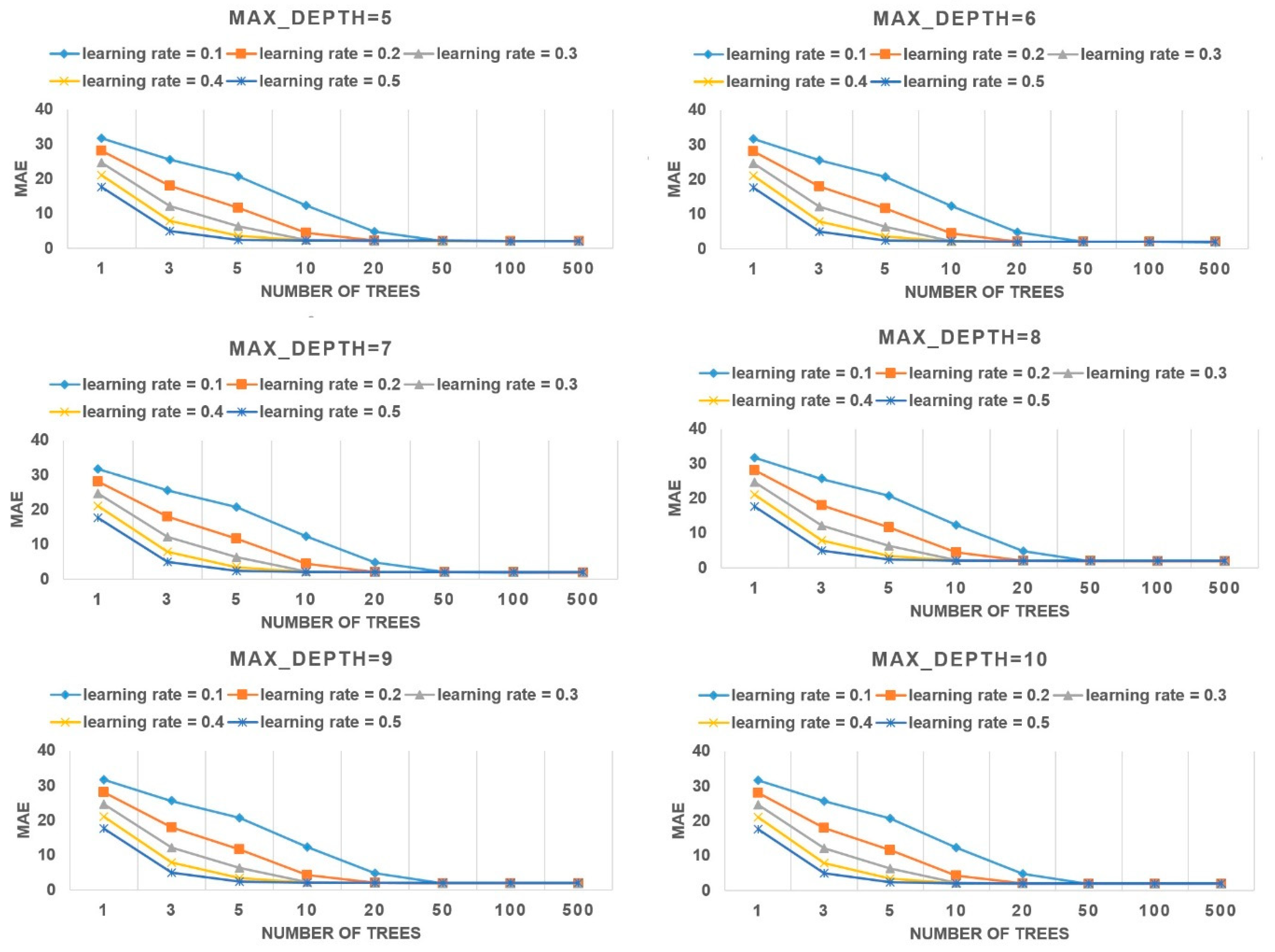
Figure 2 below shows the effects of different selected features on the prediction results.

Table 4. Detailed information on selected features.

Learning Rate	MAE
Max_depth = 5
	Number of trees
	1	3	5	10	20	50	100	500
0.1	31.623	25.610	20.744	12.355	4.863	2.107	2.086	2.017
0.2	28.105	17.999	11.645	4.437	2.164	2.110	2.081	2.032
0.3	24.589	12.169	6.374	2.361	2.143	2.111	2.092	2.054
0.4	21.077	7.916	3.586	2.192	2.169	2.140	2.113	-
0.5	17.582	5.019	2.471	2.227	2.204	2.162	2.138	-
Max_depth = 6
	Number of trees
	1	3	5	10	20	50	100	500
0.1	31.624	25.611	20.746	12.352	4.845	2.051	2.031	1.979
0.2	28.106	17.999	11.638	4.421	2.098	2.055	2.021	1.989
0.3	24.591	12.166	6.355	2.324	2.094	2.066	2.048	2.020
0.4	21.079	7.919	3.553	2.126	2.113	2.084	2.063	-
0.5	17.582	5.011	2.443	2.165	2.140	2.114	2.113	-
Max_depth = 7
	Number of trees
	1	3	5	10	20	50	100	500
0.1	31.625	25.613	20.749	12.350	4.831	2.012	1.990	1.952
0.2	28.108	18.004	11.639	4.404	2.070	2.015	1.997	1.974
0.3	24.592	12.168	6.339	2.298	2.055	2.024	2.019	2.001
0.4	21.082	7.909	3.530	2.073	2.061	2.048	2.042	-
0.5	17.586	4.995	2.392	2.089	2.075	2.072	2.064	-
Max_depth = 8
	Number of trees
	1	3	5	10	20	50	100	500
0.1	31.626	25.616	20.754	12.352	4.821	1.985	1.965	1.930
0.2	28.111	18.009	11.637	4.386	2.042	1.984	1.968	1.949
0.3	24.597	12.170	6.333	2.281	2.017	1.999	1.998	-
0.4	21.088	7.906	3.517	2.047	2.030	2.019	2.018	-
0.5	17.594	4.982	2.368	2.070	2.059	2.061	-	-
Max_depth = 9
	Number of trees
	1	3	5	10	20	50	100	500
0.1	31.629	25.620	20.757	12.351	4.807	1.963	1.941	1.915
0.2	28.117	18.016	11.639	4.375	2.012	1.956	1.945	1.935
0.3	24.606	12.171	6.322	2.256	1.992	1.977	1.971	-
0.4	21.099	7.902	3.512	2.029	2.016	2.013	-	-
0.5	17.606	4.977	2.355	2.049	2.038	2.050	-	-
Max_depth = 10
	Number of trees
	1	3	5	10	20	50	100	500
0.1	31.631	25.625	20.763	12.352	4.801	1.942	1.919	1.895
0.2	28.120	18.020	11.637	4.371	2.003	1.948	1.943	-
0.3	24.610	12.172	6.318	2.248	1.986	1.974	1.977	-
0.4	21.104	7.898	3.507	2.026	2.011	2.015	-	-
0.5	17.612	4.968	2.352	2.037	2.041	2.059	-	-

below presents the detailed prediction results including the prediction results at each step, computation time, and optimized results. The mean absolute error (MAE) is used to evaluate the performance of the model.

The equation of the MAE is provided below:

$$MAE=\frac{1}{m}{\displaystyle \sum }_{i=1}^m\left|y_i-\widehat{y_i}\right|$$

(13)

where,

$m$ = the total number of the data.

$y_i$ = the actual travel time value in the test dataset of record $i$.

$\widehat{y_i}$ = the predicted travel time value in the test dataset of record $i$.

Based on Figure 2 above, it can be concluded that the MAE value decreases as the number of trees increases, and the slopes of different learning rates are also different. In general, the lower the learning rate is, the higher the initial MAE value (with the number of tree = 1). For example, when the learning rate equals 0.1, the initial MAE value is about 36.2. In comparison, Figure 2 shows that the MAE values are about 17.6 when the number of trees is 1 and the learning rate is 0.5.

Figure 2 also shows when the number of trees reaches 50, the value of MAE becomes nearly the same. However, the data in Table 4 indicate that the results can still be optimized a little bit if the number of trees keeps increasing. Overfitting is a general problem of traditional ensemble learning methods. For example, the prediction error usually increases when the number of trees increases after it reaches the optimized point in the gradient boosting model [8]. In the XGBoost model, the overfitting problem can be solved as the algorithm will stop when there is no performance improvement after 50 iterations. Therefore, the value ‘NA’ in Table 4 means that the computation already stopped before the number of trees reached those values.

It could be seen that the parameter max_depth does not influence the prediction results significantly since the trends of the errors are nearly the same. However, the data in Table 4 show that as the max_depth increases, the MAE decreases a little bit (the optimized MAEs of max_depth from 5 to 10 are 2.02, 1.98, 1.95, 1.93, 1.91, 1.90, respectively). The data in

Table 5. Optimized prediction results and computation times.

Learning Rate	Optimized Result (MAE)	Number of Iterations	Computation Time
Max_depth = 5
0.1	2.017	500	25 min
0.2	2.032	500	25 min
0.3	2.054	500	25 min
0.4	2.079	481	23 min
0.5	2.118	217	9 min
Max_depth = 6
0.1	1.979	500	25 min
0.2	1.989	500	25 min
0.3	2.020	500	25 min
0.4	2.051	405	20 min
0.5	2.108	107	5 min
Max_depth = 7
0.1	1.952	500	25 min
0.2	1.974	500	25 min
0.3	2.001	500	25 min
0.4	2.035	231	12 min
0.5	2.064	81	4 min
Max_depth = 8
0.1	1.930	500	25 min
0.2	1.949	500	25 min
0.3	1.994	281	17 min
0.4	2.018	98	6 min
0.5	2.056	73	4 min
Max_depth = 9
0.1	1.915	500	25 min
0.2	1.935	500	25 min
0.3	1.969	167	8 min
0.4	2.012	80	4 min
0.5	2.038	70	4 min
Max_depth = 10
0.1	1.895	500	25 min
0.2	1.939	352	18 min
0.3	1.972	156	8 min
0.4	2.010	74	4 min
0.8	2.037	60	4 mins

show that as the max_depth increases, the average computation time of the model also decreases a lot, which means the larger value of max_depth can not only increase the accuracy of the model a little bit but also increase the efficiency.

According to the experimental results, it can be concluded that:

The accuracy level of a slower learning rate with a larger number of trees in the model is higher than that of a faster learning rate with a smaller number of trees. The number of trees needed to get an optimized result for the model with a faster learning rate is also lower than those with slower learning rates.

There is also a need to consider the tradeoff between prediction accuracy and computational time. Since a large number of trees is being fitted, model complexity also increases and requires more computational time. Therefore, the selection of the parameters such as max_depth and number of stopping round is important in the real world.

In addition, the maximum depth of the tree also affects the optimized selection. When the learning rates and number of trees are the same, a higher maximum depth of the tree leads to the lower error rates. A higher max_depth is also more efficient than a lower value since the number of iterations needed to achieve optimized results is lower. In general, a higher max_depth value means a more complex tree model and requires fewer trees to be fitted with a given learning rate.

4.3. Prediction Results Analysis

In the machine learning field, the predictor variables, which are the features mentioned in Table 3, usually have significant impacts on the prediction results. Exploring the influence on the individual feature can help understand the data better. Higher relative importance indicates a stronger influence in predicting travel time.

Table 6. Relative importance of each feature and their ranks in the model.

Feature	Relative Importance (%)	Rank
$T_{t-1}$	38.87	1
TOD	34.85	2
ID	12.65	3
DOW	3.76	4
Month	2.1	5
Weather	1.72	6
$\mathsf{\Delta }{T}_{t-1}^{i+1}$	0.69	7
$T_{t-1}^{i+2}$	0.6	8
$\mathsf{\Delta }{T}_{t-2}$	0.47	9
$T_{t-2}$	0.4	10
$T_{t-1}^{i-2}$	0.4	10
$\mathsf{\Delta }{T}_{t-1}^{i+1}$	0.36	12
$T_{t-3}$	0.33	13
$T_{t-1}^{i-1}$	0.29	14
$\mathsf{\Delta }{T}_{t-1}^{i-1}$	0.28	15
$\mathsf{\Delta }{T}_{t-1}^{i-2}$	0.28	15
$\mathsf{\Delta }{T}_{t-3}$	0.27	17
$T_{t-1}^{i+1}$	0.26	18
$\mathrm{L}$	0.24	19
$\mathsf{\Delta }{T}_{t-1}$	0.24	19

presents the relative importance of each feature in the optimized XGBoost model. Each predictor variable has a different impact on the predicted travel time. Based on the importance rank of each feature, it can be found that the feature $T_{t-1}$, which is the travel time at time step t−1 (15 min before), contributes the most to the predicted travel time. This result is expected and consistent with a previous study [8], which demonstrates that the immediate previous traffic condition will influence the traffic condition in the future. Therefore, this feature $T_{t-1}$ is the most important and highly correlated with the prediction value.

The results in Table 6 show that time of day is the second ranked feature with the relative importance value of 34.85%, and this result is also expected. In general, the travel time variability is also highly correlated with the time of day. The travel time usually increases a lot during peak hours and becomes stable during non-peak hours.

The third ranked feature is the segment ID with the relative importance value of 12.65%. The potential reason behind this ranking could be that the segment ID indicates which segment it is. The segment ID contains a lot of potential information such as the geographic location of the segment. Usually, different segment locations contribute to different travel time variability characteristics. Therefore, the segment ID is also a necessary and important feature in the model.

Day of the week is the 4th ranked feature in the model; the relative importance value of day of the week is 3.76%. The feature day of the week is also important in the model since the travel time is highly correlated with which day of the week it is. Based on previous studies, the traffic congestion on weekends is less frequent than on weekdays; the travel time during peak hours on Friday is usually higher than those on other weekdays [28,29]. Therefore, the feature day of the week is important in the model; this result is consistent with a previous study [8].

Weather is also considered in the model with a relative importance value of 1.72%. Inclement weather conditions may have a drastic impact on travel time variability. Therefore, the weather information is also useful in travel time prediction as adverse weather usually increases travel time. This finding is consistent with previous studies [30,31].

The travel time at time step t−1 (15 min before) is not the only feature with the consideration of temporal correlation. Several features such as the travel time of the two steps and three steps ahead (with the relative importance value of 0.40% and 0.33%, respectively) and the travel time change value of the three time steps ahead (with the relative importance value of 0.24%, 0.47%, and 0.27%, respectively) are considered in the model. These features are also used in the models of previous studies which had used gradient boosting models to predict freeway travel time [8,29]). The time change features are considered in this study because they could indicate the travel time change trends of the segments. However, the influences of these features are relatively small. The outcome is similar to the outcome of a previous study [32].

With the consideration of spatial impact, several features such as the travel time of the two upstream segments (with the relative importance value of 0.29% and 0.40%, respectively) and the travel time of the two downstream segments (with the relative importance value of 0.26% and 0.60%, respectively), one time step ahead are considered in the model. With respect to the travel time change value, the relative importance values of the two upstream segments are both 0.28%, and the relative importance values of the two upstream segments are 0.36% and 0.69%, respectively. Based on these results, it could be found that the relative importance values of the downstream segments are higher than those of upstream segments. It could be explained by the spatial characteristics of the roadway. If a bottleneck occurs at the downstream segment, the upstream segment will be influenced shortly.

In order to examine the accuracy and effectiveness of the XGBoost model, this study comprehensively evaluates the modeling results of the XGBoost model and compares the results with those of the gradient boosting model. The prediction result of the gradient boosting model is also optimized using a grid search method. For clarity, the mean absolute percentage error (MAPE) is used to evaluate and compare the performance of the two models.

The equation of the MAPE is provided below:

$$MAPE=\frac{100\%}{m}{\displaystyle \sum }_{i=1}^m\left|\frac{y_i-\widehat{y_i}}{y_i}\right|$$

(14)

where,

$m$ = The total number of the data.

$y_i$ = The actual travel time value in the test dataset of record $i$.

$\widehat{y_i}$ = The predicted travel time value in the test dataset of record $i$.

Table 7. Relative importance of each feature and their ranks in the model.

Number of Trees	MAPE XGBoost (%)	MAPE Gradient Boosting (%)
3	14.64	35.10
10	5.22	24.33
20	5.22	16.78
50	4.87	13.56
100	4.82	11.11
200	4.74	9.38
500	4.72	5.67
Average Computation Time	11.8 min	Over one hour

below presents the comparison between prediction results of the optimized XGBoost model and gradient boosting model. Based on the comparison, it could be concluded that the XGBoost model outperforms the gradient boosting model with both the consideration of accuracy and efficiency. The potential reason behind this could be as follows:

In general, the XGBoost model is a more regularized form of the gradient boosting model. XGBoost uses advanced regularization terms, which improve model generalization capabilities. Therefore, the prediction results of the XGBoost model are more accurate than those of the gradient boosting model. At the same time, the computation time of the XGBoost model (25 min) is much faster than that of the gradient boosting model (2 h). One important reason behind the better performance of the XGBoost model could be the parallel processing function. The gradient boosting model is extremely difficult to parallelize since it has sequential characteristics. In comparison, XGBoost can allow us to do the boosting work using distributed processing engines.

Another key reason is that the XGBoost model implements the early stopping function, which means that one can stop model assessment when additional trees offer no improvement to the prediction results. This function can help us not only prevent the overfitting problem, but also improve the efficiency of the model significantly.

5. Conclusions

This study aims to develop a methodology to apply the XGBoost model in travel time prediction. A real-world freeway corridor is selected as the case study to examine the XGBoost prediction model so that the gaps between the theoretical research and the application of the developed model can be bridged.

It is found that the XGBoost model can provide reliable prediction results. The relationships between several important parameters in the model (e.g., number of trees, learning rate, and maximum depth of the tree) are discussed in this study. In detail, the accuracy level of a slower learning rate with a larger number of trees in the model is higher than that of a faster learning rate with a smaller number of trees. A higher max_depth value is also more efficient than a lower value since the number of iterations needed to achieve optimized results is lower.

The relative importance of the features shows that the travel time one step ahead (15 min before) contributes the most to the predicted travel time. The features such as the time of day, day of the week and weather also have higher relative importance values in the model than other features.

The proposed XGBoost-based travel time prediction method has considerable advantages over the gradient boosting approach. The performance evaluation result shows the XGBoost-based model can have better outcomes in terms of both prediction accuracy and efficiency.

Typically, the XGBoost-based travel time prediction model can provide reliable results with low error rate. However, the impacts of accidents and roadworks on travel time prediction are also worth exploring. In the future, how to incorporate these features in the model will be studied if the data can be made available. Furthermore, the performance of the travel time prediction model is discussed under all conditions as a whole. In the future, the performances of the model under different traffic conditions (such as non-congestion conditions and congestion conditions) can be learned and compared.

References

- Wisitpongphan, N.; Jitsakul, W.; Jieamumporn, D. Travel time prediction using multi-layer feed forward artificial neural network. In Proceedings of the 2012 Fourth International Conference on Computational Intelligence, Communication Systems and Networks, Phuket, Thailand, 24–26 July 2012. [Google Scholar]
- Zheng, F.; Van Zuylen, H. Urban link travel time estimation based on sparse probe vehicle data. Transp. Res. Part C Emerg. Technol. 2013, 31, 145–157. [Google Scholar] [CrossRef]
- Wang, Z.; Fu, K.; Ye, J. Learning to estimate the travel time. In Proceedings of the 24th ACM SIGKDD International Conference on Knowledge Discovery & Data Mining, New York, NY, USA, 19–23 August 2018. [Google Scholar]
- Wang, D.; Zhang, J.; Cao, W.; Li, J.; Zheng, Y. When will you arrive? Estimating travel time based on deep neural networks. In Proceedings of the Thirty-Second AAAI Conference on Artificial Intelligence, New Orleans, LA, USA, 2–7 February 2018. [Google Scholar]
- Wei, W.; Jia, X.; Liu, Y.; Yu, X. Travel time forecasting with combination of spatial-temporal and time shifting correlation in CNN-LSTM neural network. In Proceedings of the Asia-Pacific Web (APWeb) and Web-Age Information Management (WAIM) Joint International Conference on Web and Big Data, Macau, China, 23–25 July 2018. [Google Scholar]
- Duan, Y.; Lv, Y.; Wang, F.Y. Travel time prediction with LSTM neural network. In Proceedings of the 2016 IEEE 19th International Conference on Intelligent Transportation Systems (ITSC), Rio de Janeiro, Brazil, 1–4 November 2016. [Google Scholar]
- Hamner, B. Predicting travel times with context-dependent random forests by modeling local and aggregate traffic flow. In Proceedings of the 2010 IEEE International Conference on Data Mining Workshops, Sydney, Australia, 13 December 2010. [Google Scholar]
- Zhang, Y.; Haghani, A. A gradient boosting method to improve travel time prediction. Transp. Res. Part C Emerg. Technol. 2015, 58, 308–324. [Google Scholar] [CrossRef]
- Li, X.; Bai, R. Freight vehicle travel time prediction using gradient boosting regression tree. In Proceedings of the 2016 15th IEEE International Conference on Machine Learning and Applications (ICMLA), Anaheim, CA, USA, 18–20 December 2016. [Google Scholar]
- Fan, S.K.S.; Su, C.J.; Nien, H.T.; Tsai, P.F.; Cheng, C.Y. Using machine learning and big data approaches to predict travel time based on historical and real-time data from Taiwan electronic toll collection. Soft Comput. 2018, 22, 5707–5718. [Google Scholar] [CrossRef]
- Gupta, B.; Awasthi, S.; Gupta, R.; Ram, L.; Kumar, P.; Prasad, B.R.; Agarwal, S. Taxi travel time prediction using ensemble-based random forest and gradient boosting model. Adv. Big Data Cloud Comput. 2018, 645, 63–78. [Google Scholar]
- Yu, B.; Wang, H.; Shan, W.; Yao, B. Prediction of bus travel time using random forests based on near neighbours. Comput. Aided Civ. Infrastruct. Eng. 2018, 33, 333–350. [Google Scholar] [CrossRef]
- Wu, C.H.; Ho, J.M.; Lee, D.T. Travel-time prediction with support vector regression. IEEE Trans. Intell. Transp. Syst. 2004, 5, 276–281. [Google Scholar] [CrossRef] [Green Version]
- Banfield, R.E.; Hall, L.O.; Bowyer, K.W.; Kegelmeyer, W.P. A comparison of decision tree ensemble creation techniques. IEEE Trans. Pattern Anal. Mach. Intell. 2006, 29, 173–180. [Google Scholar] [CrossRef] [PubMed]
- LeBlanc, M.; Tibshirani, R. Combining estimates in regression and classification. J. Am. Stat. Assoc. 1996, 91, 1641–1650. [Google Scholar] [CrossRef]
- Alajali, W.; Zhou, W.; Wen, S.; Wang, Y. Intersection traffic prediction using decision tree models. Symmetry 2018, 10, 386. [Google Scholar] [CrossRef] [Green Version]
- Dong, X.; Lei, T.; Jin, S.; Hou, Z. Short-term traffic flow prediction based on XGBoost. In Proceedings of the 2018 IEEE 7th Data Driven Control and Learning Systems Conference (DDCLS), Enshi, China, 25–27 May 2018. [Google Scholar]
- Myung, J.; Kim, D.K.; Kho, S.Y.; Park, C.H. Travel time prediction using K Nearest Neighbor method with combined data from vehicle detector system and automatic toll collection system. Transp. Res. Rec. J. Transp. Res. Board 2011, 2256, 51–59. [Google Scholar] [CrossRef]
- Liu, Y.; Wang, Y.; Yang, X.; Zhang, L. Short-term travel time prediction by deep learning: A comparison of different LSTM-DNN models. In Proceedings of the 2017 IEEE 20th International Conference on Intelligent Transportation Systems (ITSC), Yokohama, Japan, 16–19 October 2017. [Google Scholar]
- Moonam, H.M.; Qin, X.; Zhang, J. Utilizing data mining techniques to predict expected freeway travel time from experienced travel time. Math. Comput. Simul. 2019, 155, 154–167. [Google Scholar] [CrossRef]
- Kearns, M. Thoughts on Hypothesis Boosting. 1988. Available online: http://www.nzdl.org/cgi-bin/library.cgi?e=d-00000-00---off-0coltbib--00-1----0-10-0---0---0direct-10---4-------0-1l--11-en-50---20-about---01-3-1-00-0-0-11-1-0utfZz-8-00&a=d&d=k-thb-88&showrecord=1 (accessed on 31 July 2021).
- Rajsingh, E.B.; Veerasamy, J.; Alavi, A.H.; Peter, J.D. Advances in Big Data and Cloud Computing; Springer: Berlin/Heidelberg, Germany, 2018; Volume 645. [Google Scholar]
- Friedman, J.H. Greedy function approximation: A gradient boosting machine. Ann. Stat. 2001, 29, 1189–1232. [Google Scholar] [CrossRef]
- Freeman, E.A.; Moisen, G.G.; Coulston, J.W.; Wilson, B.T. Random forests and stochastic gradient boosting for predicting tree canopy cover: Comparing tuning processes and model performance. Can. J. For. Res. 2015, 46, 323–339. [Google Scholar] [CrossRef] [Green Version]
- Chen, T.; Guestrin, C. Xgboost: A scalable tree boosting system. In Proceedings of the 22nd ACM Sigkdd International Conference on Knowledge Discovery and Data Mining, San Francisco, CA, USA, 13–17 August 2016. [Google Scholar]
- Min, W.; Wynter, L. Real-time road traffic prediction with spatio-temporal correlations. Transp. Res. Part C Emerg. Technol. 2011, 19, 606–616. [Google Scholar] [CrossRef]
- Wang, Y.; Zhang, Y.; Piao, X.; Liu, H.; Zhang, K. Traffic data reconstruction via adaptive spatial-temporal correlations. IEEE Trans. Intell. Transp. Syst. 2018, 20, 1531–1543. [Google Scholar] [CrossRef]
- Chen, X.M.; Chen, X.; Zheng, H.; Chen, C. Understanding network travel time reliability with on-demand ride service data. Front. Eng. Manag. 2017, 4, 388–398. [Google Scholar] [CrossRef]
- Chen, P.; Tong, R.; Lu, G.; Wang, Y. Exploring travel time distribution and variability patterns using probe vehicle data: Case study in Beijing. J. Adv. Transp. 2018, 2018, 3747632. [Google Scholar] [CrossRef] [Green Version]
- Qiao, W.; Haghani, A.; Shao, C.F.; Liu, J. Freeway path travel time prediction based on heterogeneous traffic data through nonparametric model. J. Intell. Transp. Syst. 2016, 20, 438–448. [Google Scholar] [CrossRef]
- Koesdwiady, A.; Soua, R.; Karray, F. Improving traffic flow prediction with weather information in connected cars: A deep learning approach. IEEE Trans. Veh. Technol. 2016, 65, 9508–9517. [Google Scholar] [CrossRef]
- Cheng, J.; Li, G.; Chen, X. Research on travel time prediction model of freeway based on gradient boosting decision tree. IEEE Access 2018, 7, 7466–7480. [Google Scholar] [CrossRef]
Figure 1.
Selected I-77 segments.
Figure 2.
XGBoost travel time prediction model outputs.