
How Retailer Co-Opetition Impacts Pricing, Collecting and Coordination in a Closed-Loop Supply Chain


1
College of Economics & Management, Huazhong Agricultural University, Wuhan 430070, China
2
Research Center of Hubei Logistics Development, Hubei University of Economics, Wuhan 430205, China
3
International Business School Suzhou, Xi’an Jiaotong-Liverpool University, Suzhou 215123, China
4
DeGroote School of Business, McMaster University, Hamilton, ON L8S4M4, Canada
*
Author to whom correspondence should be addressed.
Sustainability 2021, 13(18), 10025; https://0-doi-org.brum.beds.ac.uk/10.3390/su131810025
Submission received: 10 July 2021
/
Revised: 2 September 2021
/
Accepted: 3 September 2021
/
Published: 7 September 2021
(This article belongs to the Section Waste and Recycling)
Abstract
:The cooperative and competitive (i.e., co-opetition) behavior between retailers plays a significant role in the development of operations and marketing strategies in a supply chain. Specifically, retailers’ co-opetition relationship pivotally influences the sustainable performance in a closed-loop supply chain. This study examines the impact of retailer co-opetition on pricing, collection decisions and coordination in a closed-loop supply chain with one manufacturer and two competing retailers. Based on observations in some industries (e.g., electronic manufacturing, fabric and textile, etc.), the cooperative and competitive relationships between retailers can be classified into the following three different modes: Bertrand competition, Stackelberg competition, and Collusion. In this paper, we establish a centralized and three decentralized game-theoretic models under these three co-opetition modes and characterize the corresponding equilibrium outcomes. The results indicate that the Bertrand competition mode yields the highest return rate, which is also superior to the other two modes for both the manufacturer and the supply chain system in terms of profitability. However, it can be shown that which mode benefits the retailers would depend on the degree of competition between the retailers and the relative remanufacturing efficiency. Interestingly, we find that the retailer’s first-move advantage does not necessarily lead to higher profits. In addition, we design a modified two-part tariff contract to coordinate the decentralized closed-loop supply chains under three different retailer co-opetition modes, and the results suggest that the optimal contractual parameters in the contracts highly rely on the remanufacturing efficiency and the competition degree between the two retailers. Several managerial insights for firms, consumers and policy makers are provided through numerical analysis.
1. Introduction
The implementation of closed-loop supply chain (CLSC) strategies can save production costs for manufacturers while improving the environmental and social benefits of the supply chain [1,2,3]. In recent years, driven by the economic benefits from remanufacturing and government regulations, it is observed that an increasing number of well-known manufacturers and retailers have implemented the CLSC strategies, which has played a significant role in achieving harmonious development of economy, society and, environment. For example, as stated in Apple’s 2018 Environmental Responsibility Report, the firm’s goal was to build a CLSC that would ensure a sustainable way of production by using recycled or renewable materials while strengthening cooperation with its suppliers, distributors and recyclers to improve the efficiency of the product recycling and remanufacturing (https://www.apple.com/cn/environment/pdf/Apple_Environmental_Responsibility_Report_2018.pdf, accessed on 15 June 2021).
In practice, it is not uncommon to observe that manufacturers or retailers in a CLSC may be engaged in cooperative and competitive relationships simultaneously. One example for such relationships are electronics manufacturers (e.g., Apple, Huawei) who, on the one hand, are competing in selling smartphones and tablets through the common retailers such as Suning, Jindong and Gome; on the other hand, they also cooperate in the operation of recycling used products through online recycling platforms (e.g., Aihuishou, Huishoubao) (http://www.sohu.com/a/198707207_507050, accessed on 15 June 2021). The existence of the combined cooperation and competition (referred to as co-opetition structure) in a supply chain affects not only the strategic interactions between supply chain members, but also the channel power of upstream manufacturers and downstream retailers. This paper focuses on investigating the pricing, collecting decisions and coordination in CLSCs with the consideration of the retailer co-opetition behavior.
With the development of the internet and information technology, it leads to the emergence of new business models such as new retailing and omni-channel retailing, in which retailers actively seek to cooperate in terms of making operations and marketing strategies, instead of focusing solely on competition. For example, Yonghui announced the establishment of a strategic partnership with Advantage, whereby its subsidiaries Yonghui Holdings and BCE will absorb shares of Daman International in a new DN company at a ratio of 40% and 60%, respectively, in exchange for a 20% stake in KTLP which is wholly owned by Advantage. This strategic partnership, if realized, will give birth to the world’s largest retailing service company (http://finance.sina.com.cn/stock/usstock/c/2017-11-16/doc-ifynstfi0029811.shtml, accessed on 15 June 2021). In November 2017, Alibaba, Auchan Retail and Rundai Group formed a new retail strategic partnership, in which Alibaba intends to invest approximately HK$22.4 billion to indirectly own 36.16% of Gao Xin Retail (http://www.sohu.com/a/210700427_99934114, accessed on 15 June 2021).
In the CLSC context, it is noteworthy that the competition and cooperation among retailers not only influences the forward wholesaling and retailing processes, but also has strategic impacts on the efficiency of used product collection, which may ultimately affect firms’ profit. Hence, it would be of great theoretical and practical significance to analyze the impacts of the different retailer co-opetition modes (i.e., Bertrand competition, Stakerlberg competition and collusion) on the pricing and collecting decisions of CLSCs. In addition, it is worthwhile to explore how the CLSC coordination under different retailer co-opetition modes can be realized by means of designing appropriate contracts. The existing studies regarding pricing strategies and coordination operations in CLSCs are based primarily on the assumption of an independent retailer [4,5,6,7]. Few studies extend the no competition case to the competition case by taking into account two competitive retailers [8,9,10,11]. In contrast to the above studies, this article aims to fill a research gap by examining the strategic role of the retailer co-opetition in the operations strategies and coordination in a CLSC. Specifically, we aim to address the following research questions:
- What are the equilibrium wholesale prices, retail prices, and return rates of CLSCs under different retailer co-opetition modes?
- Which retailer co-opetition mode is more beneficial to the manufacturer, retailers, and entire supply chain system in a CLSC?
- How to design rational contracts so as to achieve the coordination of decentralized CLSCs under different retailer co-opetition modes?
To answer the above questions, we establish game-theoretic models for a CLSC consisting of a manufacturer and two retailers. The two retailers might choose to compete or cooperate in the consumer market. We model three game scenarios based on the co-opetition behavior of the two retailers, namely Bertrand competition, Stackelberg competition and Collusion. It is assumed that the manufacturer acts as the channel leader in all the CLSC models. We characterize the optimal co-opetition mode selection strategies for the manufacturer, retailers and supply chain system. Then, based on the optimal results of the centralized CLSC model, we design rational coordination contracts for the decentralized CLSCs under retailer co-opetition.
The results show that the Bertrand competition mode is the most beneficial for the manufacturer as well as the supply chain system. This is mainly due to the fact that the degree of retailer competition is more pronounced in the Bertrand mode than that of the Stackelberg and Collusion modes, thus resulting in highest demand and return quantity among the three modes. However, which mode benefits the retailers is relatively complicated because we show that the result depends on the following two key factors: the degree of retailer competition and the manufacturer’s relative remanufacturing efficiency. More importantly, we find that the retailer who has the first-move advantage may not necessarily achieve higher profit for itself. In fact, it turns out that the retailer might even benefit from losing its first-move advantage. Moreover, to mitigate the double marginalization effect of the decentralized CLSCs, we show that the modified two-part tariff contracts can perfectly coordinate the supply chain, and the manufacturer can extract higher increased profits from channel coordination in the Bertrand competition mode.
The remainder of this paper is organized as follows. Section 2 reviews the related literature. Section 3 establishes a centralized and three decentralized CLSC models. Section 4 derives the equilibrium solutions for the four CLSC models built in Section 3. Section 5 compares the equilibrium price and collection decisions as well as profits for the four CLSC models. Section 6 presents several numerical examples. Section 7 concludes the study, summarizes managerial insights and points out several future research directions. All proofs are relegated to the Appendix A and Appendix B.
2. Literature Review
Our work is closely related to three streams of research that study the impacts of retailer co-opetition on supply chains, pricing and collecting decisions in CLSCs, and CLSC coordination.
2.1. The Impacts of Retailer Co-Opetition on Supply Chains
This study complements the existing literature that addresses the effects of retailer co-opetition behavior on supply chain decisions. Prior research has extensively explored pricing, quantity and vertical bargaining problems with differentiated retailers. Choi [12] considers both the manufacturer competition and retailer competition channel structures, and analyzes the impacts of horizontal product differentiation and store differentiation on manufacturer’s and retailer’s profits. Padmanabhan and Png [13] study the manufacturer’s return strategies with competing retailers and analyze the effects of demand uncertainty and retailer competition in supply chain decisions. With the rapid development of e-commerce and the internet, some scholars focus on sales channel competition. For example, Chiang et al. [14], Hsiao and Chen [15], Zhou and Zhao [16], Modak and Kelle [17], Li et al. [18] study the strategic impacts of introducing the direct channel on pricing decisions and supply chain performance, while Abhishek et al. [19], Tian et al. [20], Li and Wei [21] consider the e-tailers’ channel selection between reselling and agency selling modes. However, the above-mentioned studies focus on decisions made in the retailer competition or sales channel competition environments while completely ignoring the cooperation factor between retailers. In the co-opetition modeling context, Xiong et al. [22], Aust and Buscher [23], Chutani and Sethi [24] investigate the vertical cooperative advertising strategies in a supply chain with competing retailers. Similarly, Hosseini-Motlagh et al. [25] consider retailers’ co-opetition behavior and supply chain coordination where the demand depends on promotion efforts and trade credits.
2.2. Pricing and Collecting Decisions in CLSCs
This study also contributes to an emerging body of literature on pricing and collecting decisions in CLSCs. Previous research explores the pricing and collecting decisions of CLSCs in a noncompetitive environment [4,5,6]. Later, some researchers extended the problem to the competitive settings. Savaskan and Van Wassenhove [8] study the interplay between product pricing in forward supply chain and manufacturer’s reverse channel selection with competing retailers. They consider two collection modes, namely direct collecting and indirect collecting, and analyze the drivers of manufacturer’s reverse channel selection decisions. Yi et al. [26] investigate the impacts of power structure on prices and corresponding profits in a CLSC with retailers engaging in Cournot competition. Wei and Zhao [9] study pricing and collecting decisions under retailer competition and fuzzy demand.
In addition, Wu and Zhou [10], Li et al. [27] extend the model considered by Wei and Zhao [9] to the case of CLSC competition. Regarding the cooperation behavior in CLSCs, Jena and Sarmah [28] consider a CLSC model of competing manufacturers selling products to a common retailer. They also examine the impacts of the vertical cooperation between manufacturers and retailers on pricing and return rate decisions. Wang et al. [29] focus on a CLSC model with competitive recycling channels, and they find that the manufacturer always chooses manufacturer remanufacturing while the recycling channel selection depends on the unit cost of self-collecting and the compensation from outsource collecting. Wang et al. [11] show how retailers’ potential collusion behavior can affect the supply chain performance with a monopolistic manufacturer and two competing retailers. They find that the collusion always benefits retailers while at risk of harming the environment and social welfare.
2.3. CLSC Coordination
Operations managers are becoming increasingly interested in designing relevant contracts (e.g., revenue-sharing contract, two-part tariff contract or cost-sharing contract etc.) so that the improvement and coordination in CLSCs can be achieved. Under a monopolistic environment, Shi et al. [30] derive a scheme for coordinating a CLSC under retailer’s risk-averse behavior. Xiong et al. [31] design an improved contract (i.e., revenue and cost sharing contract) to coordinate a CLSC with technology licensing. Choi et al. [6] consider the channel power structure and verify the validity of the revenue sharing contract or the two-part tariff contract in coordinating the CLSCs. Heydari et al. [32] show that a reverse/closed-loop supply chain can increase sustainable competitiveness when the government designs relevant incentive contracts to motivate consumers to return their used products. Panda and Modak [33] find that the revenue sharing contract can perfectly coordinate a socially responsible CLSC. Recent papers have extended the CLSC coordination problems by incorporating the information asymmetry [34,35]. Under the context of a competitive framework, Savaskan and Van Wassenhove [8] design a contract consisting of wholesale price, transfer buy-back price and fixed slotting fee, which effectively coordinate the CLSC with competing retailers. Zheng et al. [7], Zheng et al. [36] show that the dual-channel CLSC coordination under different power structures (i.e., manufacturer-led, retailer-led, and third-party-led power structures) and recycling channel modes (i.e., manufacturing-collecting, retailer-collecting, and third-party-collection modes) can be achieved. Similarly, Yi and Yuan [37], Xie et al. [38], Taleizadeh et al. [39], Zhang et al. [40], Liu et al. [41] show that suitable coordination contracts can essentially be used as a strategic tool to mitigate the conflict between direct and retail channels.
2.4. Research Gaps and Our Contributions
Based on the above-mentioned three streams of literature that are closely related to this study, we summarize the research gaps and main contributions of our study in the following three aspects.
First, unlike the existing studies on investigating the impacts of retailer co-opetition on supply chains that mainly consider the forward supply chains, we incorporate the used product collection and remanufacturing into manufacturer’s decision making. Specifically, we examine the problem setting where the manufacturer wholesales products to the two retailers with different co-opetition behaviors.
Second, different from the aforementioned studies in which there is solely competition in the CLSCs, we consider the case where there exists simultaneous cooperation and competition between the retailers. Furthermore, we identify certain situations under which the retailers might be worse off from the first-move advantage.
Third, unlike the existing studies on the CLSC that focus on the cases of a monopolistic retailer or two competitive retailers, we study the case where two the retailers might engage in either competition or corporation relationship in a CLSC, and we explore how to design appropriate contracts to coordinate CLSCs under different co-opetition behaviors between the retailers. We also identify the situation where it is easier for the manufacturer to implement channel coordination in CLSCs. In particular, we show that these considerations provide valuable insights into the pricing and collecting decisions when the product remanufacturing strategy is implemented.
We further compare our study with the related literature in Table 1.
3. The Model
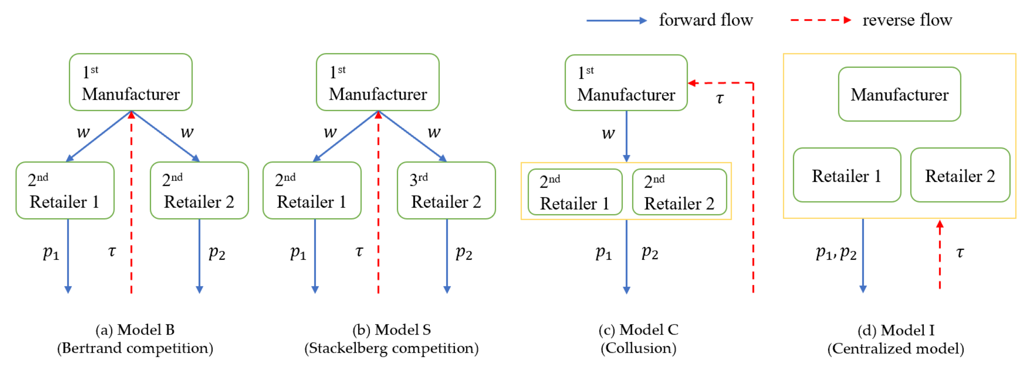
We consider a CLSC that includes the forward and reverse collection flows, consisting of one manufacturer and two competing retailers (referred to as Retailer 1 and Retailer 2). In the forward flow, the manufacturer wholesales the product to the retailers at a price ; Retailer 1 (respectively, Retailer 2) then sells the product to the consumer market at a price (respectively, ). In the reverse flow, the manufacturer collects the used product directly from the market by itself. Such a collection mode has been widely adopted in today’s industrial practice. For example, Apple sells its electronic products (e.g., iPhone, iPad and Apple Watch) through online retailers such as Jindong and Tmall, and also directly collects the used products through “trade-in” service on its own official website (https://www.apple.com/cn/shop/trade-in, accessed on 15 June 2021).
Let and be the unit production cost of manufacturing the new product and remanufactured product, respectively. Both the survey and existing literature suggest that remanufacturing a product is less costly than manufacturing a new product, i.e., [5,7,42]. Focusing on investigating how retailer co-opetition would affect the CLSC’s decisions and profits, we further assume that there is no distinction between the new and remanufactured products, which is commonly adopted in the CLSC literature and also consistent with many remanufacturing practices [4,5]. Let () be the return rate (i.e., the percentage of the collection quantity to the market demand), then the corresponding total collection cost can be characterized as a function of the return rate, i.e., , where is a scaling parameter. The above-mentioned quadratic collection cost function suggests that the collection cost is convexly increasing in the return rate. Note that the similar cost functions have been widely used in the CLSC literature [4,7]. Denote (i.e., ) by the unit remanufacturing cost saving [43], thus the average production cost can be written as .
Assume that the products produced by Retailer 1 and Retailer 2 are imperfect substitutes, and they are engaged in price competition. The demand functions for both retailers are given by (This demand function is deduced from the quadratic consumption utility of a representative consumer, which is specified as .):
where and are the sales quantities of Retailer 1 and Retailer 2, respectively; and are the retail prices charged by Retailer 1 and Retailer 2, respectively. The parameter captures the degree of competition (also referred to as the degree of product differentiation) between the two retailers. Specifically, if , the products sold by the two retailers are independent. In contrast, indicates that their products are close to perfect substitutes. As increases, the degree of competition between Retailer 1 and Retailer 2 increases. Similar linear demand functions are widely used in economics and marketing literature [19,44].
With the above model assumptions regarding the costs and demands, the profits for the manufacturer and retailers in the CLSC are given as
where ,, and and denote the manufacturer’s and Retailer ’s profits, respectively.
Next, we depict three decentralized CLSC models under different retailer co-opetition modes, namely the CLSC model with retailer Bertrand competition (Model B, Figure 1a), the CLSC model with retailer Stackelberg competition (Model S, Figure 1b), and the CLSC model with retailer collusion (Model C, Figure 1c). When the two retailers are in Bertrand competition, they make price decisions (i.e., and ) simultaneously. If Retailer 1 and Retailer 2 are in a leader–follower Stackelberg competition, without loss of generality, we assume that Retailer 1 acts as the leader and determines the price , and Retailer 2 acts as the follower and determines the price . Finally, for the Collusion model, Retailer 1 and Retailer 2 form an alliance and jointly determine the prices and to maximize their total profits. To provide a benchmark for supply chain coordination, we also construct a centralized CLSC model (Model I, Figure 1d) where the manufacturer and the two retailers centrally determine the price and return rate decisions.
For notational convenience, let be the channel member ’s profit in the decision-making case , where denotes the manufacturer, retailer and supply chain system, respectively; denotes the Bertrand competition, Stackelberg Competition, Collusion, centralized and supply chain coordination models, respectively. In addition, we define the following equations: , , , , . All proofs are relegated to the Appendix A and Appendix B. Table 2 summarizes the notations used throughout this paper.
4. CLSC Models with Retailer Co-Opetition
In this section, we establish a centralized and three decentralized CLSC models under retailer co-opetition. Then, the corresponding equilibrium solutions and optimal profits for all the four CLSC models are obtained. We begin by analyzing the centralized CLSC model.
4.1. Centralized Model (Model I)
In the benchmark Model I, the manufacturer and the two retailers jointly make the pricing and collecting decisions so as to maximize the channel-wide profit. In this model, the wholesale price can be viewed as an internal transfer price, which would not affect the supply chain’s optimal decisions. Hence, the centralized decision-making system determines , and to optimize the entire supply chain profit:
Because the objective function is jointly concave in , and , solving the simultaneous first-order conditions yields the optimal solutions for the Model I. The optimal prices (i.e., and ), optimal return rate (i.e., ), and optimal profit (i.e., ) are shown in the Column “Model I” of Table 3. The derivation process of the Model I is presented in Appendix A. It should be noted that the return rate is between 0 and 1, thus we impose the condition on the return rate , which is in consistent with the Assumption 9 by Savaskan et al. [4].
Lemma 1.
The scaling parameterdefined in the collection cost function should satisfy the condition , such that .
Lemma 1 indicates that the remanufacturing is sufficiently costly for the manufacturer, thus it is not economically viable to remanufacture all used products [4,6]. The optimal solutions of the Model I show that the optimal retail prices reduce as the remanufacturing cost saving (i.e., ) increases while increasing as the scaling parameter (i.e., ) decreases. Because consumers could benefit from the lower price and higher market demand led by a higher remanufacturing cost saving or a lower collection cost, manufacturers should strategically increase their investments in recycling and remanufacturing activities to improve the efficiency of product reuse.
4.2. Retailers Engage in Bertrand Competition (Model B)
In the Model B, Retailer 1 and Retailer 2 engage in Bertrand competition, that is, they determine their retail prices simultaneously. In this case, Retailer 1 and Retailer 2 have balanced power and make pricing decisions based on the manufacturer’s optimal wholesale price decision. The sequence of events is as follows. First, the manufacturer determines the wholesale price and return rate . Then, Retailer 1 and Retailer 2 determine the retail prices and , respectively. This can be modeled as a leader–follower Stakelberg game, and the backward induction method is used to solved this model. The derivation process of the Model B is given in Appendix A.
For a given and , Retailer 1 and Retailer 2 seek to maximize their respective profit:
Because is concave in , and is concave in , the retailers’ best response functions can be obtained by solving the first-order conditions, which are given by . Given and , the manufacturer’s problem can be stated as follows:
From the concavity of the manufacturer’s objective function in and , we obtain the optimal wholesale price and optimal return rate . Then, by substituting and into the retailers’ best response functions, the optimal retail prices and are obtained. Finally, we can compute the channel members’ and supply chain’s optimal profits , () and , which are shown in the Column “Model B” of Table 3.
4.3. Retailers Engage in Stackelberg Competition (Model S)
It is not uncommon to observe that competing retailers in a supply chain may have unequal channel power when making their pricing decisions. For example, the giant retailers (e.g., Walmart, JD.com) often compete with some small local retailers in selling the same products. When Retailer 1 and Retailer 2 are engaged in Stackelberg competition, in general, Retailer 1 has the first-move advantage than Retailer 2 in terms of making pricing decisions. The sequence of events is as follows. First, the manufacturer acts as the leader, determining the wholesale price and in anticipation of the retailers’ decisions. Next, Retailer 1 chooses its retail price based on the manufacturer’s optimal decisions. Finally, Retailer 2 determines its retail price based on the manufacturer’s and Retailer 1′s optimal decisions. From the concavity of the Retailer 2′s objective function as shown in Equation (7), the first-order condition yields its best response .
Given , and , Retailer 1 optimizes its own profit:
Because the objective function is concave in , the best response for Retailer 1 can be derived from its first-order condition, which is given by . Then, Retailer 1’s best response can be transferred into , which now only depends on the variable . For a given and , the manufacturer’s optimization problem is
From the first-order conditions, the manufacturer determines the optimal wholesale price and optimal return rate , from which the optimal retail prices and , optimal profits for all channel members , and , and optimal profit for the supply chain are obtained, which are shown in the Column “Model S” of Table 3.
4.4. Retailers Engage in Collusion-Model C
In the Model C, Retailer 1 and Retailer 2 collude to determine the retail prices. Compared with Bertrand and Stackelberg competition models, the retailers’ pricing power is strengthened in the Collusion model. The sequence of events is as follows. The manufacturer first chooses the wholesale price and return rate in anticipation of the retailers’ decisions. Then, Retailer 1 and Retailer 2 jointly determine the retail prices and based on the manufacturer’s optimal decisions. For a given and , Retailer 1 and Retailer 2 jointly optimize the following problem:
where denotes the total profit of Retailer 1 and Retailer 2 in the Model C. From the concavity of the objective function in Equation (11) in terms of and , the simultaneous solutions of the first-order conditions yield the best responses for the two retailers, which are given by: . Given and , the manufacturer determines the wholesale price and return rate by solving the following optimization problem:
Because the objective function in Equation (12) is concave in and , the optimal wholesale price and optimal return rate in the Model C can be derived from the first-order conditions of Equation (12). Then, the optimal prices (i.e., and ) and the optimal profits for the channel players and supply chain (i.e., , () and ) are shown in the Column “Model C” of Table 3.
5. Comparison of the Four CLSC Models
In this section, we compare the optimal prices, return rates and profits under the centralized and three decentralized CLSC models so as to analyze the effects of retailer co-opetition on the CLSC decisions. Specifically, we aim to investigate which supply chain model could lead to the highest return rate, and which supply chain mode, from the perspectives of the manufacturer and retailers, is more preferable.
Lemma 2.
The optimal wholesale prices in the three decentralized CLSC models satisfy the following relationship:.
It should be noted that the manufacturer’s optimal wholesale price decision highly hinges on its channel power in the supply chain. When Retailer 1 and Retailer 2 engage in the Bertrand competition, the manufacturer is more powerful because the degree of competition is sufficiently high compared to that under the Stackelberg competition and Collusion modes. Hence, the manufacturer has enough incentives to set a lower wholesale price, which would motivate the retailers to lower the retail prices. This suggests that a lower wholesale price is the most effective way to improve the channel demand in this case. In contrast, when Retailer 1 and Retailer 2 collude to determine the retail prices, the relative channel power of the manufacturer reduces while the alliance of the two retailers becomes stronger. In such a case, the manufacturer would increase the wholesale price to reduce the disadvantage resulting from the retailers’ collusion. In summary, Lemma 2 suggests that the stronger relative channel power would provide stronger incentive for the manufacturer to lower the wholesale price to the retailers.
Lemma 3.
(1) The equilibrium retail prices in the centralized and three decentralized CLSC models are related as follows:. Correspondingly, the equilibrium demands satisfy the following relationship:
(2) The total demands of the two retailers in the centralized and three decentralized CLSC models are related as follows: .
Note that the retailers’ decisions depend upon the manufacturer’s wholesale price and return rate decisions. From Lemma 2, we observe that the manufacturer would charge a higher wholesale price in the Collusion model, thus the retailers respond by increasing retail prices. In addition, the investments in collection activity would induce the retailers to reduce the retail prices because the cost savings from the remanufacturing can be indirectly reflected in the retail prices.
We also find that the reduction in retail prices is more pronounced in the Bertrand model than that found in the other two CLSC models, which explains why the Bertrand model achieves the lower retail prices. In addition, notice that in the Stackelberg model, Retailer 1 sets a higher retail price than that of Retailer 2. The intuition is that Retailer 1 has the first-move advantage over Retailer 2, and thus it has the ability to set a higher retail price. Finally, the retail prices are lower in the centralized model because there is no double marginalization effect in the centralized decision-making system.
In terms of the market demand, it is interesting to observe that Retailer 2′s demand is higher than that of Retailer 1 under the Stackelberg competition model. The intuition is that Retailer 2, who acts as the follower, would strategically determine a lower retail price to increase the demand in the Stackelberg competition model. Moreover, it is noteworthy that Retailer 2′s demand in the Model S could be higher than that under the centralized model, which hinges on the degree of retailer competition (i.e., ). Specifically, when is sufficiently high, Retailer 2′s demand is higher than that in the centralized model, demonstrating that in the presence of retailer competition, the first-move advantage of the dominant retailer does not always make it better off. In addition, it is worth mentioning that the centralized model may not always lead to higher demands for the two retailers than that of the decentralized model.
Lemma 3(2) highlights the fact that a lower retail price would lead to a higher market demand. Notice that the Bertrand competition model achieves the lower retail prices, which in turn increases the market demand of the supply chain. However, when Retailer 1 and Retailer 2 collude, the total demand of the two retailers is reduced as the two retailers are more monopolistic.
Proposition 1.
The equilibrium return rates in the centralized and three decentralized CLSC models are related as follows:.
Note that the manufacturer’s incentives in the collection activity is determined by the total cost savings from the remanufacturing, which can be represented by , where . Recall that Lemma 3 indicates that the total demand in the Bertrand competition model is higher than that in the other two decentralized models. Hence, the manufacturer should prefer to make more investments in collecting used products when Retailer 1 and Retailer 2 are engaged in Bertrand competition model. In other words, the investment in the collection activity would be the most effective way to increase the remanufacturing cost saving in the Bertrand competition case. In contrast, the manufacturer would have a lower incentive to increase the investments in the collection under the Collusion model due to the lower demand. Intuitively, the centralized model is optimal, and it also could achieve a higher return rate than that in the three decentralized CLSC models.
Our results shed some lights on the operations and marketing strategies for the firms in the CLSC. The results indicate that it is more efficient for the manufacturer’s investment in the collection activities if the retailers become more competitive. Notice that in the Bertrand competition model, the effective loss of channel efficiency, to a certain extent, is mitigated by an increased demand. Hence, as a response, the manufacturer should take the retailer co-opetition behavior into consideration when making collection decisions. The manufacturer’s investment in collecting the used product collection should be increased when the retailers are more competitive (i.e., in the Bertrand competition model) and reduced when the retailers become more monopolistic (i.e., in the Collusion model). Moreover, because increasing the collection quantity would generate more social and environmental benefits, the policy makers should design relevant regulations to encourage the retailer competition (or restrict the collusion between the retailers) in the CSLC.
Proposition 2.
The manufacturer’s optimal profit in the centralized and three decentralized CLSC models are related as follows:. Consequently, the optimal profit of the entire supply chain system in the four CLSC models satisfy the following relationship:.
Proposition 2 analyzes how retailer co-opetition affects the manufacturer’s and entire supply chain’s profits. Note that both the total demand and the return rate are higher under the Bertrand competition model compared with the other two models (see Lemma 3), thus both the manufacturer and entire supply chain obtain higher profit under the Bertrand competition model. It is straightforward that retailer collusion results in a lower collection quantity and demand for the manufacturer and supply chain system, which in turn makes them worse off compared with the Bertrand and Stackelberg competition models. Note also that the centralized model leads to the highest profit because all the decision variables reach their optimal values.
Because it is analytically challenging to make the direct comparison of the retailers’ optimal profit under different configurations, we first define an effective factor, allowing us to investigate which co-opetition model is more beneficial to the retailers.
The effective factor corresponds to the ratio between square of the remanufacturing cost saving (i.e., ) and the collection cost scale parameter (), measuring the relative remanufacturing efficiency for the manufacturer. Obviously, a higher value of could be achieved by increasing the remanufacturing cost savings (i.e., ) or by decreasing the collection cost scale parameter (i.e., ). For ease of exposition, we define the following functions:
Proposition 3.
The retailer’s optimal profit in the centralized and three decentralized CLSC models are related as follows:
where, , , , .
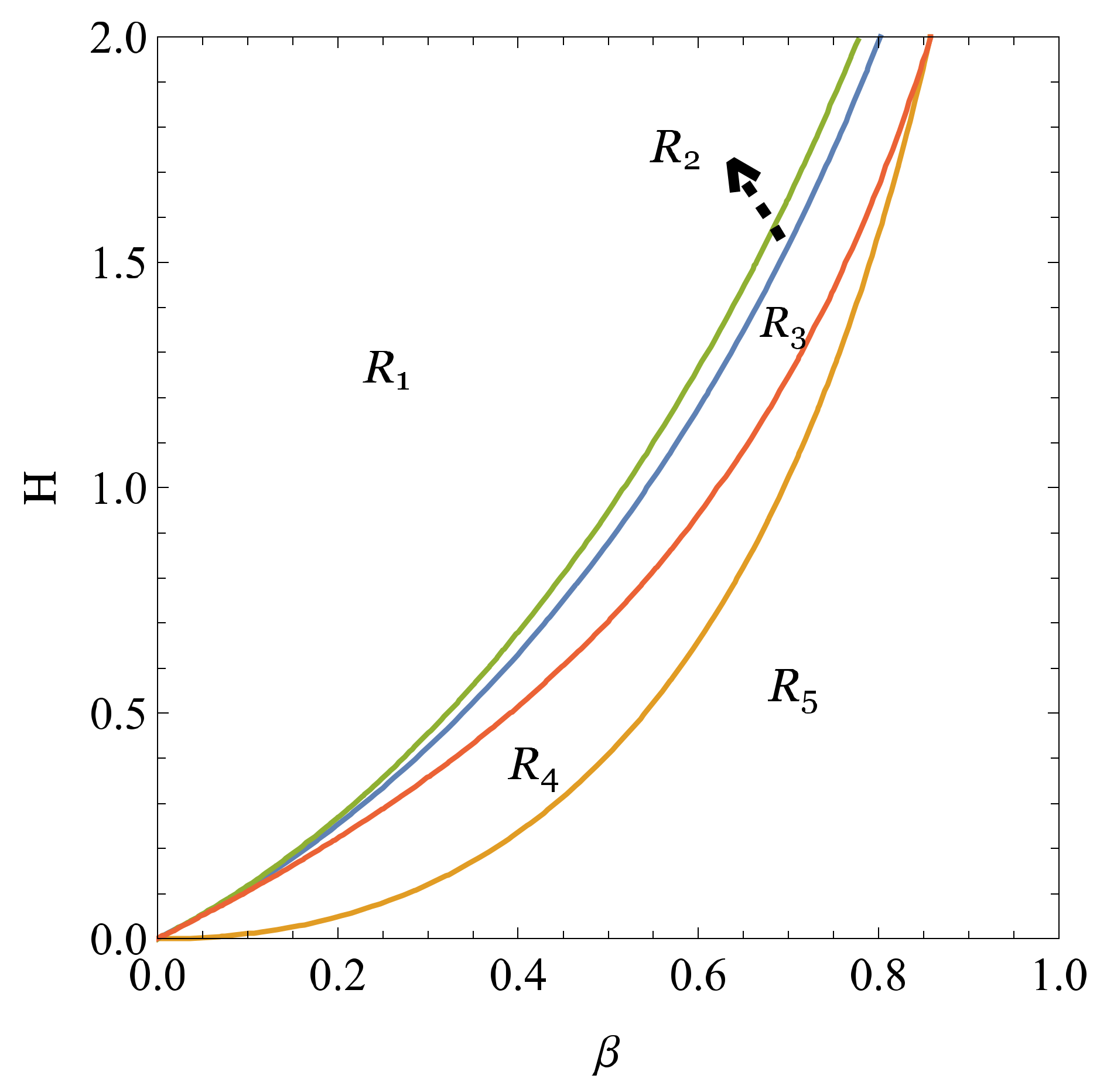
Proposition 3 indicates that when the relative remanufacturing efficiency () is sufficiently high while the degree of retailer competition () is sufficiently low, Retailer 2′s profit in the Stackelberg competition model is higher than that in the other two models. However, as the degree of retailer competition decreases, the profit advantage of Retailer 2 gradually shrinks. The intuition is that the retailers’ profit mainly hinges on the margin profit of the product and the sales quantity. When the two retailers are sufficiently differentiated (i.e., is small) and the remanufacturing efficiency is relatively high, the manufacturer is more willing to provide a lower wholesale price to the retailers in a such way to stimulate the market demand. In this case, the demand plays a dominant role and thus the retailers could obtain higher profit in the Collusion model than that in the Stackelberg competition model. In contrast, when increases (see Region in Figure 2), the Collusion model is preferable for the retailers due to the decreased profit margin in the Bertrand competition model. Particularly, in the Stackelberg competition model, we find from Proposition 2 that Retailer 2, who acts as the follower, achieves a higher profit than Retailer 1. This is mainly due to the fact that Retailer 2 can strategically adjust its price decision based on Retailer 1′s retail price, which results in a higher demand (see Lemma 2). Such a result further demonstrates that the first-move advantage does not necessarily bring a corresponding higher profit for the retailer in the Stackelberg competition model.
Proposition 3 also highlights the fact that the Collusion model is more favorable for the retailers when is sufficiently large while is relatively small; however, the profit benefit reduces as the collection cost scale parameter increases. This is because even though the market demand is lower in the Collusion model than that in the other two models, the retailers can still obtain the higher profits through setting the higher retail prices, which leads to the higher profit margins for the retailers. Notice also that as the relative remanufacturing efficiency increases, the manufacturer can strategically increase the wholesale price, which can effectively limit the retailers’ pricing advantage in the Collusion model. The findings in Proposition 3 reveal certain managerial insights for the retailers’ operations and marketing strategies. In the context of the CLSC, the retailers should take into full consideration both the relative remanufacturing efficiency and the degree of competition when making pricing decisions. The retailer cooperation could be an effective way of limiting the manufacturer’s wholesale price advantage, while such a limiting effect is reduced as the relative remanufacturing efficiency increases.
6. Coordination of Three Decentralized CLSC Models
Our above analysis has shown that the supply chain profit yielded by the decentralized models cannot achieve the optimal profit as in the centralized model because of the well-known double marginalization effect presented in the decentralized supply chains. Therefore, we take the equilibrium decisions in the centralized as a benchmark to design effective contracts coordinating the decentralized CLSCs under different retailer co-opetition configurations. Following Savaskan et al. [4] and Choi et al. [6], we propose an improved contract based on the traditional two-part tariff contract to coordinate the three decentralized CLSCs. Then, we examine the impact of retailer co-opetition on the contractual parameters of the CLSC.
We focus on a CLSC consisting of one manufacturer and two competing retailers. In essence, the retailer co-opetition configuration affects the coordination mechanism design of the CLSC. In the Bertrand and Collusion models, the two retailers simultaneously determine the retail prices. The supply chain can be viewed as a parallel structure with a Stackelberg leader (i.e., manufacturer) and two first-level “in parallel” followers (i.e., Retailer 1 and Retailer 2). However, in the Stackelberg competition mode, the two retailers determine the retail price sequentially and the supply chain is a serial chain with a Stackelberg leader (i.e., manufacturer), a first-level follower (i.e., or subleader, Retailer 1), and a second-level follower (i.e., Retailer 2) [6]. In the following, we explore how to coordinate the parallel and serial CLSCs through designing effective supply chain contracts.
In the parallel CLSCs (i.e., Model B and Model C), the implementation of the improved two-part tariff contract is described as follows. First, the manufacturer, who serves as the channel leader, commits to offering a lower wholesale price (compared to the decentralized cases) to the retailer and sets the same return rate as that in the centralized model. Second, Retailer 1 and Retailer 2 pay the manufacturer a fixed fee and , respectively, to compensate for the revenue reduction of the manufacturer. By implementing the improved two-part tariff contact in the CLSC, the manufacturer’s optimization problem is as follows:
In the above optimization problem, Equations (15) and (16) are the retailers’ individual rationality constraints which ensure that the contract offered by the manufacturer will be accepted by the retailers. The manufacturer’s and retailers’ compatibility constraint Equation (17) ensures both parties choose the optimal decisions as those in the centralized model. The constraint Equation (18) guarantees that the wholesale price and fixed payments in the contracts are non-negative.
Differing from the parallel configuration, the improved two-part tariff contract in the serial CLSC (Model S) is implemented as follows. First, Retailer 1 provides Retailer 2 a subcontract () which is a combination of the retail price and a fixed payment, and Retailer 2 sets the optimal retail price ; subsequently, the manufacturer offers Retailer 1 the contract () which consists of the wholesale price and a fixed payment and sets the optimal return rate . Therefore, the manufacturer in the serial CLSC optimizes the following problem:
By solving the above two optimization problems for the manufacturer, we obtain the optimal contracts of the CLSC under different retailer co-opetition modes, which are shown in the following proposition.
Proposition 4.
In the mode , where the optimal wholesale prices and fixed payments in the improved two-part tariff contracts are shown inTable 4. In addition, in the contract (), the optimal retail prices and return rates are the same as those in the centralized model , , , and the entire supply chain system profit also attains the optimal level, .
Proposition 5 shows that the improved two-part tariff contract can effectively coordinate the CLSCs under different retailer co-opetition models. In such a contract, the manufacturer and the two retailers all choose the optimal retail prices as those in the centralized model so that the demand and system profit are maximized, and the double marginalization effect of the decentralized CLSC is eliminated. In addition, from the perspectives of channel players (i.e., manufacturer, Retailer 1 and Retailer 2), the retailers obtain the reservation profits in the decentralized models (i.e., , ,), while the manufacturer obtains all the increased profit from the supply chain coordination (i.e., ). Thus, despite the fact that the implementation of the contract could lead to the optimal system performance, it actually does not provide sufficient incentive for the retailers to accept the contact. To tackle this issue, a complementary contract (e.g., profit-sharing contract, Nash bargaining contract) can be used to reallocate the increased profit, ensuring that the manufacturer and the two retailers are all better off.
Note that the optimal parameters (i.e., wholesale prices and fixed transfer payments) in the supply chain coordination contracts under different retailer co-opetition modes are not the same. Then, it is worthwhile to investigate how retailer co-opetition mode affects the optimal parameters in the two-part tariff contracts.
Proposition 5.
In the three retailer co-opetition models, the optimal contractual wholesale prices satisfy , and the optimal fixed transfer payments satisfy
where,,.
Proposition 5 suggests that retailer co-opetition model could affect the optimal contractual parameters (i.e., the optimal wholesale prices and the optimal fixed transfer payments , where ). Note that the optimal wholesale price in the contracts is the highest in the Bertrand competition model while the lowest in the Collusion model, which is contrary to the result found in the decentralized models (i.e., ). This result can be explained as follows. In the Collusion mode, the two retailers’ bargaining power is relatively strong, and as a result, the manufacturer should lower the wholesale price in order to achieve the channel coordination. On the contrary, the retailers’ bargaining power is relatively weak in the Bertrand competition mode, thus the manufacturer would prefer a higher wholesale price to coordinate the decentralized CLSCs.
As the manufacturer charges a higher wholesale price in the Bertrand competition model, the optimal fixed transfer payment in this case is comparatively lower. When comparing the three configurations, the supply chain efficiency satisfies the following relationship, , indicating that the Bertrand competition model would lead to the highest channel efficiency compared with the other two models. Moreover, the optimal fixed transfer payments under the Collusion and Stackelberg competition models hinge on the retailer competition intensity (i.e., ) and the relative remanufacturing efficiency (i.e., ), which suggests that the manufacturer should flexibly adjust the fixed payment charged to the retailers based on the retailer co-opetition mode and relative remanufacturing efficiency.
7. Numerical Analysis
In this section, we present several numerical examples to explore the effects of some key parameters on CLSC decisions and supply chain contracts. Considering the constraints stated in the early sections, we set the initial parameter set based on the initial parameter values as given in Zheng et al. [45]. Let , and . The numerical results are shown in Figure 3, Figure 4, Figure 5, Figure 6 and Figure 7. In the following, we analyze the effects of the retailer competition intensity (i.e., ) on the equilibrium prices, demands and return rates under different CLSC models.
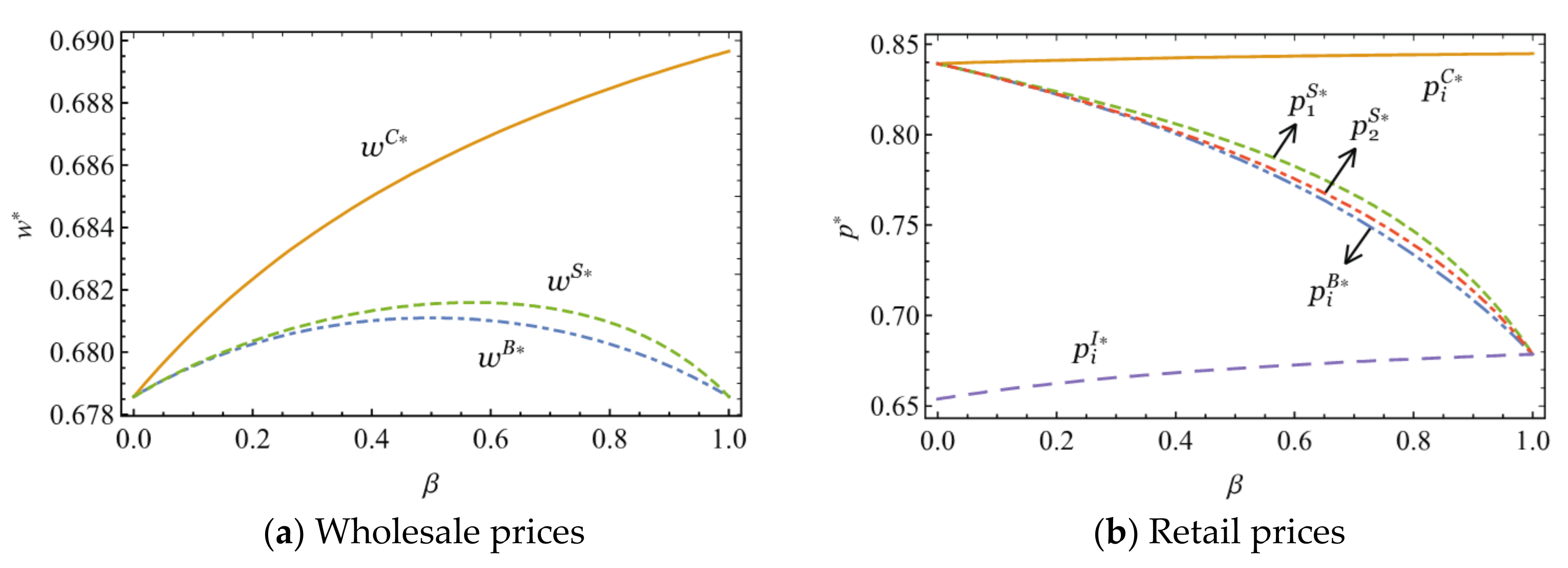
Figure 3a shows that the manufacturer would charge the highest wholesale price in the Collusion model and the lowest price in the Bertrand competition model, which confirms with the results in Proposition 1. In addition, it is observed that the optimal wholesale price is increasing with in the Collusion configuration while exhibiting concavity behavior (i.e., first increasing and then decreasing) with in the Stackelberg and Bertrand competition configurations. This can be explained by the fact that in the Collusion case, the manufacturer can increase its revenue by lowering the wholesale price, with an increase in . However, in the Stackelberg and Bertrand competition cases, the manufacturer may choose to increase the wholesale price to improve the profit margin when is low, and to reduce the wholesale price when is moderate or high. From Figure 3b, we find that the optimal retail prices increase with in the centralized and Collusion models, and decrease with in the Stackelberg and Bertrand competition models, indicating that when the retailers form an alliance (i.e., Model I and Model C), they have more incentives to raise the prices as the degree of competition increases.
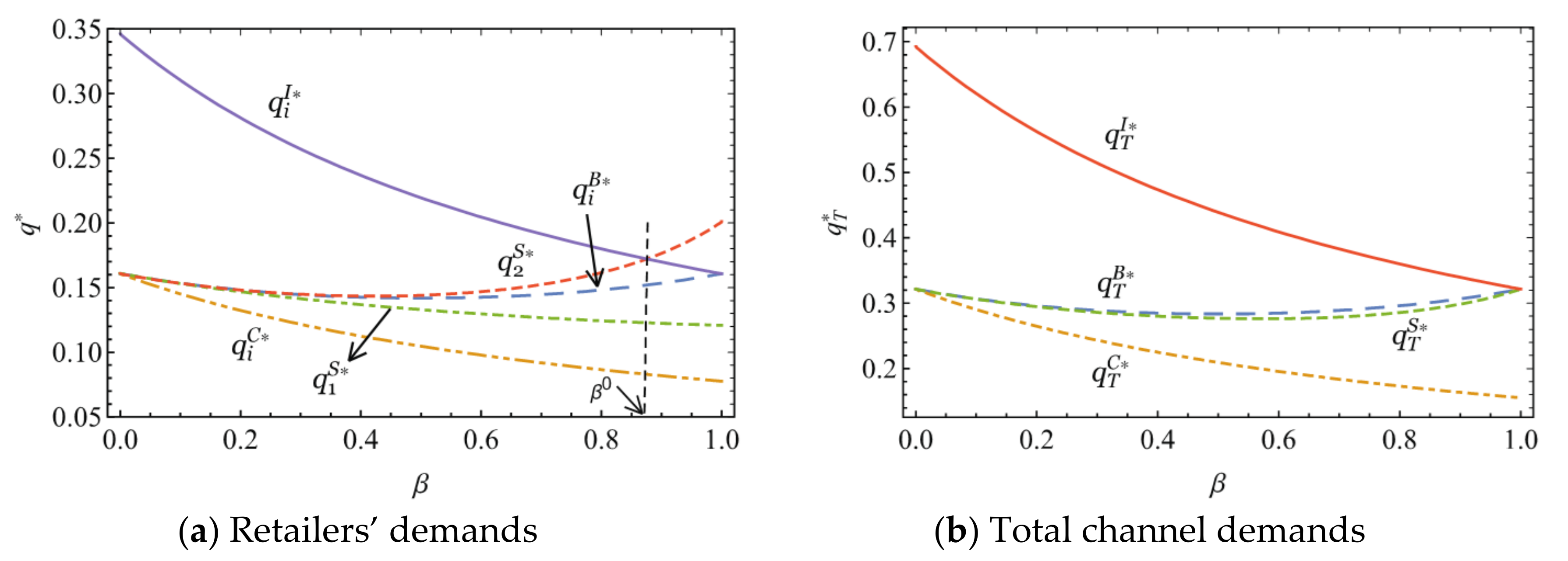
Figure 4 investigates the impact of on the equilibrium demands of Retailer 1 and Retailer 2. We see that in the Collusion and centralized models, the demands decrease with due to the increasing retail prices (see Figure 3b). For the two retailers in the Bertrand model and Retailer 2 in the Stackelberg model, notice that the demands first decrease and then increase with . From the perspective of the total demand, it decreases with in the centralized and Collusion models, and it first decreases and then increases with in the Bertrand and Stackelberg models. The managerial insights for the results are as follows. The fiercer competition between the retailers does not necessarily result in a lower demand (e.g., in the Bertrand model). In addition, the second-move retailer in the Stackelberg model would respond to increase the demand because is sufficiently high, which confirms the second-move advantage for the retailer in the CLSC with competing retailers.
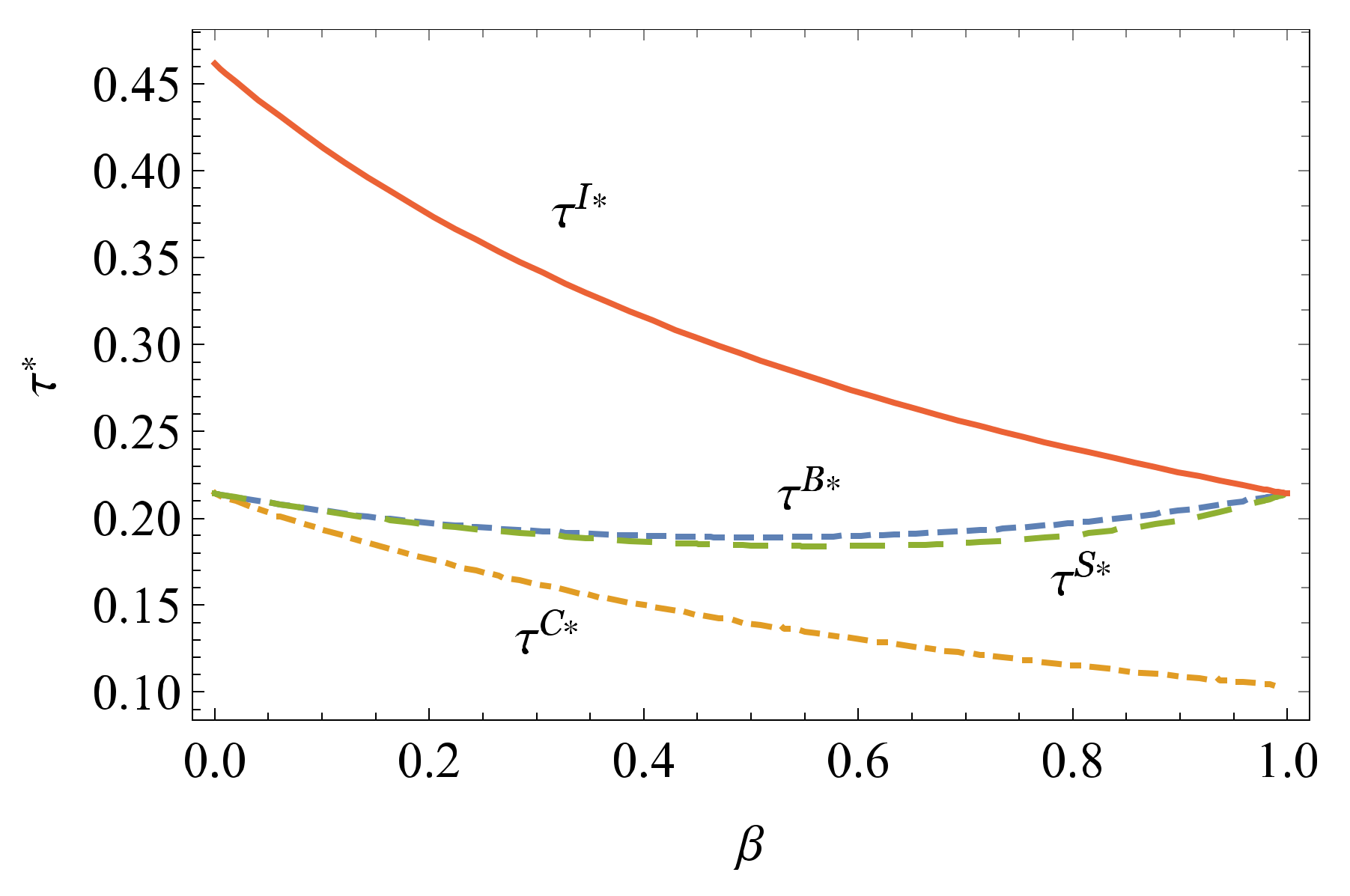
Figure 5 examines the impact of on the equilibrium return rates (i.e., , where ). First, we find that the centralized model attains the highest return rate; in the decentralized models, the return rate is higher in the Bertrand competition case and lower in the Collusion case. Second, it is seen that and are decreasing with due to the decreased demands from the higher (see Figure 4b), whereas and are of the similar behaviors as their corresponding market demand shapes.
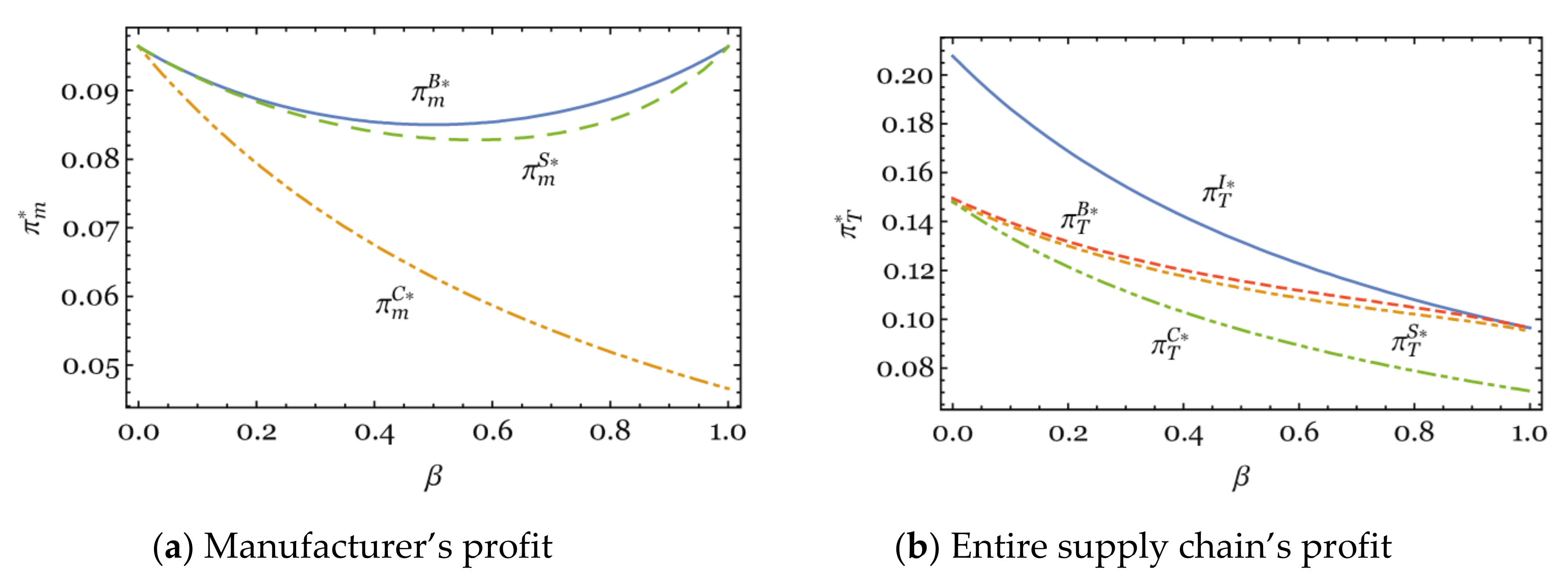
Figure 6 analyzes the impact of retailer competition intensity (i.e., ) on the manufacturer’s and supply chain system’s profits. It is observed that the manufacturer obtains the lowest profit in the Collusion model and the highest profit in the Bertrand model, which coincides with the results in Proposition 4. In addition, the manufacturer’s profit decreases with in the Collusion model, while first decreasing and then increasing in the Bertrand and Stackelberg models. For the supply chain system, it is interesting to see that the system’s profit decreases with under the three decentralized CLSC models, regardless of whether the manufacturer’s profit is monotonically related to or not. The intuition is that the retailer’s profit plays a dominant role in determining the system’s profit.
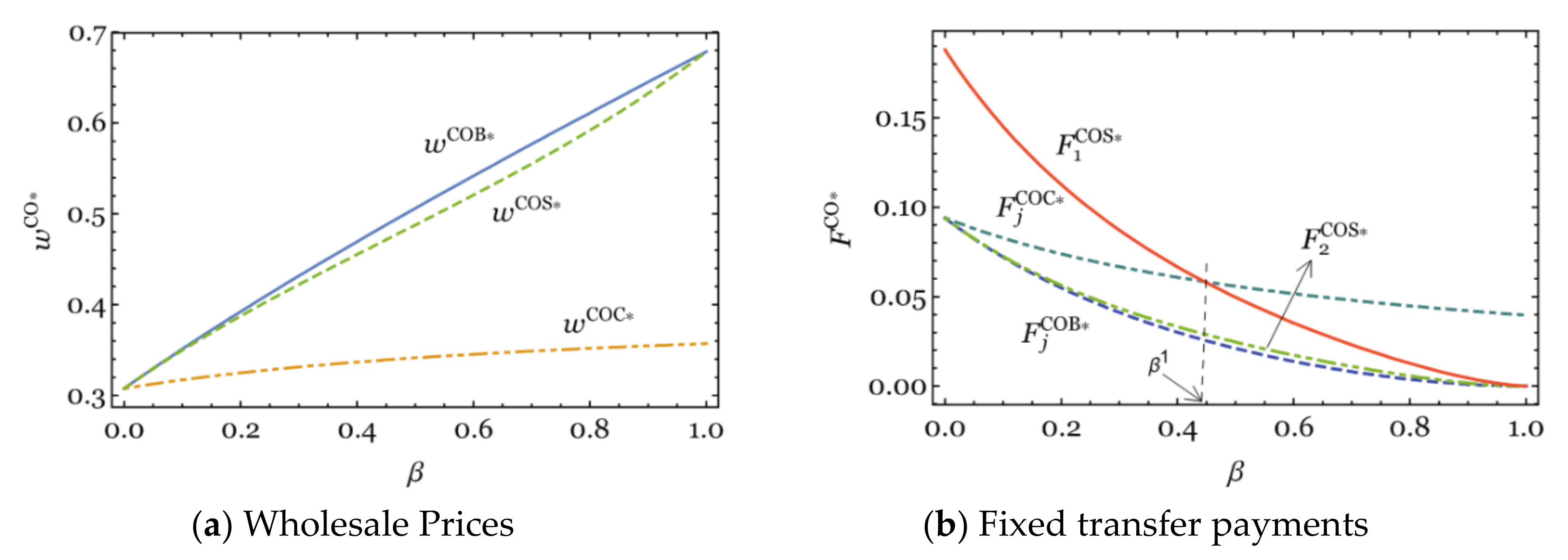
Figure 7 analyzes the impact of retailer competition intensity on the contractual parameters (i.e., the wholesale price and fixed transfer payment ). As can be seen in Figure 7a, the wholesale prices under the coordination are the highest in the Bertrand model and the lowest in the Collusion model. The result suggests that the manufacturer would increase the wholesale price in the coordination as increases, which, to some extent, can effectively mitigate the double marginalization effect of the CLSC. Figure 7b shows that the optimal fixed transfer payments under the different CLSC models decrease with , indicating that the manufacturer would cost less to achieve the CLSC coordination when the competition intensity between the two retailers increases.
8. Conclusions
In this paper, we study retailer co-opetition behavior in a CLSC consisting of a manufacturer and two competing retailers. The manufacturer sells its products through the retailers and is also responsible for collecting the used products from the consumer market. Based on the cooperative and competitive relationships between the retailers, three different retailer co-opetition modes (Bertrand competition, Stackelberg competition and collusion) have been considered.
By establishing the decentralized models of the three modes and comparing the equilibrium results, we analyze the impacts of the retailer co-opetition behavior on pricing, collecting decisions and profits in the CLSC. The results show that the Bertrand model could achieve a higher return rate compared with the other two models (i.e., Stackelberg and Collusion models); correspondingly, the manufacturer and the supply chain system can also attain higher profit in this competition model. In contrast, the retailers’ profit under different models hinges on their competition intensity and the manufacturer’s relative remanufacturing efficiency. In addition, we find that all the three decentralized CLSC models cannot achieve the optimal efficiency as in the centralized model. Hence, we design the modified two-part tariff contract to coordinate CLSC models under different channel settings. Specifically, we find that the contractual wholesale price is the highest, while the fixed transfer payment is the lowest in the Bertrand competition model.
Our findings provide important managerial implications for manufacturers, retailers, consumers and policy makers. First, the manufacturers should incentivize the retailers to increase the competition level, through which the market demand and collection quantity are both increased. Moreover, as the channel leader, the manufacturer can voluntarily achieve CLSC coordination by designing a modified two-part tariff contract. Second, we find that the retailers should strategically adjust their competition and cooperation modes based on the market condition and the manufacturer’s relative remanufacturing efficiency because the competition does not always lead to a worse situation for them. Third, our results suggest that consumers should voluntarily return used products to the manufacturer because the remanufacturing cost saving can be reflected in the retail price, and this positive effect is maximized when retailers engage in Bertrand competition. Finally, the policy makers should set relevant policies to encourage the competition and avoid the collusion behavior between retailers, thus improving the return rate and environmental performance.
We briefly note here several limitations of this paper and provide some avenues for future research. First, we explicitly assume that the new product and remanufactured product are identical to the consumers. However, in practice, the new and remanufactured products are commonly differentiable, and consumers also have different willingness to pay for them. Hence, it would be interesting to establish alternative CLSC models by incorporating product differentiation. Second, it would be practical if we also consider the co-opetition behavior between upstream manufacturers and further investigate the impacts of manufacturer co-opetition on the pricing and collection decisions in the CLSC. Third, our study considers a two-echelon CLSC consisting of a manufacturer and two competing retailers, it would be interesting yet challenging to examine the pricing and collection decisions in the context of multi-echelon CLSCs. Finally, we have not considered the impacts of the uncertainty (e.g., demand and cost uncertainties) on the CLSC, it is worthwhile to investigate the interplay between the retailer co-opetition and cost/demand uncertainty in the CLSC, and we leave this direction for future research.
Author Contributions
Conceptualization, B.Z.; Funding acquisition, B.Z.; Methodology, X.L., G.H. and B.Z.; Supervision, J.C. and B.Z.; Validation, G.H., J.C. and K.H.; Writing—original draft, X.L.; Writing—review & editing, G.H., J.C., B.Z. and K.H. All authors have read and agreed to the published version of the manuscript.
Funding
This research was supported in part by the National Natural Science Foundation of China (72101208), the Natural Science Foundation of Hubei Province (2019CFB120), the Fundamental Research Funds for the Central Universities (2662020JGPYG14, BC2021119), the Philosophy and Social Science Project of Hubei Province (20G032), and Provincial Innovation and Entrepreneurship Training Program for Undergraduate (S202110504139).
Institutional Review Board Statement
Not applicable.
Informed Consent Statement
Not applicable.
Data Availability Statement
The authors confirm that this research is original, free of plagiarism and adheres to COPE’s Code of Conduct and Best Practice Guidelines.
Conflicts of Interest
All authors declare no conflict of interest in this paper.
Appendix A. The Derivations of the Four CLSC Models
For notational convenience, recall that we defined , , , , in Section 3.
The derivation of Model I:
According to Equation (5), we obtain the Hessian Matrix as follows:
Let denote the leading principal minor of the matrix . Then the corresponding determinants are , ,. To ensure is negative definite, the condition (i.e.,) needs to satisfied. Then, the first-order conditions of the supply chain are as follows:
Jointly solving the above equations, we derive the equilibrium outcomes of Model I:
Moreover, the optimal profit can then be calculated.
The derivation of Model B:
According to Equations (6) and (7), , hence is concave in and is concave in . The first-order conditions result in the retailers’ best response functions:
Then, the manufacturer’s objective function, conditional on the retailers’ best response functions, is given by Equation (8). The Hessian Matrix of the manufacturer is as follows:
Note that when the condition is satisfied, is jointly concave in and . Then, the simultaneous first-order conditions result in the manufacturer’s optimal decisions:
Then, the optimal retail prices and , optimal profits of channel members and supply chain are obtained, which are shown in Table 2.
The derivation of Model S:
Because is concave in , Retailer 2′s best response function is . Plugging into the Retailer 1′s objective function yields Equation (9). The second-order partial derivative is , is concave in and the first-order condition results in . Then, the manufacturer’s objective function is given in Equation (15); the Hessian Matrix is given as follows:
It can be verified that when the condition is satisfied, is jointly concave in and and . Then, the simultaneous first-order conditions result in the manufacturer’s optimal decisions:
Then, the optimal retail prices and , optimal profits of channel members and supply chain are obtained, which are shown in Table 2.
The derivation of Model C:
According to Equation (11), the Hessian Matrix of is given as follows:
is jointly concave in and . The first-order conditions result in . Then, according to the manufacturer’s objective function, which is given in Equation (12), the Hessian Matrix of the manufacturer is given by
When the condition is satisfied, is jointly concave in and . The first-order conditions result in the manufacturer’s optimal decisions:
Then, the optimal retail prices and , optimal profits of channel members and supply chain are obtained, which are shown in Table 2.
Appendix B. Proofs of Lemmas and Propositions
Proof of Lemma 1.
In the Model I, to ensure the optimal return rate , the condition needs to be satisfied. Furthermore, note that also can guarantee the concavity of the manufacturer’s objective functions in Model B, Model S and Model C. □
Proof of Lemma 2.
From Table 2, we have , because , ; in addition,
.
Then, Lemma 2 is proved. □
Proof of Lemma 3.
Figure A1.
Effects of and on .

Figure A1 shows that is always positive, hence . In addition,
We can verify that is always positive, hence, .
In summary, . In a similar way, we can prove , where . □
Proof of Proposition 1.
We have
Then, . Proposition 1 is proved. □
Proof of Proposition 2.
We have
hence, . In a similar way, we can prove .
Then, Proposition 2 is proved. □
Proof of Proposition 3.
Section 5 (Pages 16–17) has shown the detailed derivation proofs for Proposition 3; we omit the proof here. □
Proof of Proposition 4.
In the Bertrand competition model (Model B), to achieve CLSC coordination, the best response function of the retail price in Equation (5) needs to satisfy , where . Hence, we have
Under the contract, retailers obtain reservation profit, i.e., where . Hence,
similarly, we obtain . After we obtain the optimal contract , the equilibrium outcomes and profits can be derived.
In a similar way, we can prove the optimal contracts under the Collusion and Stackelberg models. □
Proof of Proposition 5.
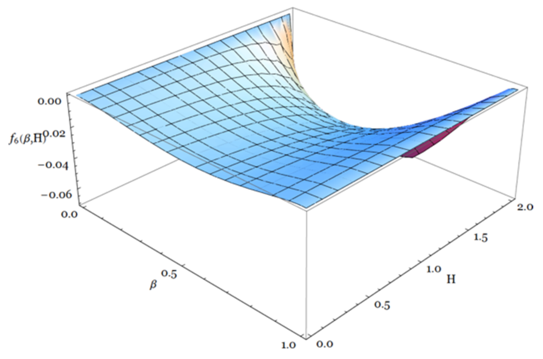
We have
Let , which is depicted in Figure A2. Hence, , . In a similar way, we can prove when and when . Then, Proposition 5 is proved. □
Figure A2.
Effects of and on .

References
- Wu, C.H.; Kao, Y.J. Cooperation regarding technology development in a closed-loop supply chain. Eur. J. Oper. Res. 2018, 267, 523–539. [Google Scholar] [CrossRef]
- Gaur, J.; Subramoniam, R.; Govindan, K.; Huisingh, D. Closed-loop supply chain management: From conceptual to an action oriented framework on core acquisition. J. Clean. Prod. 2017, 167, 1415–1424. [Google Scholar] [CrossRef]
- Polat, L.O.; Gungor, A. WEEE closed-loop supply chain network management considering the damage levels of returned products. Environ. Sci. Pollut. Res. 2021, 28, 7786–7804. [Google Scholar] [CrossRef] [PubMed]
- Savaskan, R.C.; Bhattacharya, S.; Van Wassenhove, L.N. Closed-loop supply chain models with product remanufacturing. Manag. Sci. 2004, 50, 239–252. [Google Scholar] [CrossRef] [Green Version]
- Atasu, A.; Toktay, L.B.; Van Wassenhove, L.N. How collection cost structure drives a manufacturer’s reverse channel choice. Prod. Oper. Manag. 2013, 22, 1089–1102. [Google Scholar] [CrossRef]
- Choi, T.M.; Li, Y.; Xu, L. Channel leadership, performance and coordination in closed loop supply chains. Int. J. Prod. Econ. 2013, 146, 371–380. [Google Scholar] [CrossRef]
- Zheng, B.; Chu, J.; Jin, L. Recycling channel selection and coordination in dual sales channel closed-loop supply chains. Appl. Math. Model. 2021, 95, 484–502. [Google Scholar] [CrossRef]
- Savaskan, R.C.; Van Wassenhove, L.N. Reverse channel design: The case of competing retailers. Manag. Sci. 2006, 52, iv-154. [Google Scholar] [CrossRef] [Green Version]
- Wei, J.; Zhao, J. Pricing decisions with retail competition in a fuzzy closed-loop supply chain. Expert Syst. Appl. 2011, 38, 11209–11216. [Google Scholar] [CrossRef]
- Wu, X.; Zhou, Y. The optimal reverse channel choice under supply chain competition. Eur. J. Oper. Res. 2017, 259, 63–66. [Google Scholar] [CrossRef]
- Wang, Q.; Hong, X.; Gong, Y.; Chen, W.A. Collusion or Not: The optimal choice of competing retailers in a closed-loop supply chain. Int. J. Prod. Econ. 2020, 225, 107580. [Google Scholar] [CrossRef]
- Choi, S.C. Price competition in a duopoly common retailer channel. J. Retail. 1996, 72, 117–134. [Google Scholar] [CrossRef]
- Padmanabhan, V.; Png, I.P.L. Manufacturer’s return policies and retail competition. Mark. Sci. 1997, 16, 81–94. [Google Scholar] [CrossRef]
- Chiang, W.K.; Chhajed, D.; Hess, J.D. Direct marketing, indirect profits: A strategic analysis of dual-channel supply-chain design. Manag. Sci. 2003, 49, v-142. [Google Scholar] [CrossRef] [Green Version]
- Hsiao, L.; Chen, Y.J. Strategic motive for introducing internet channels in a supply chain. Prod. Oper. Manag. 2014, 23, 36–47. [Google Scholar] [CrossRef]
- Zhou, J.H.; Zhao, R.J. Dual-channel signaling strategy with channel competition. Syst. Eng.-Theory Pract. 2018, 38, 414–428. [Google Scholar]
- Modak, N.M.; Kelle, P. Managing a dual-channel supply chain under price and delivery-time dependent stochastic demand. Eur. J. Oper. Res. 2019, 272, 147–161. [Google Scholar] [CrossRef]
- Li, J.; Yi, L.; Shi, V.; Chen, X. Supplier encroachment strategy in the presence of retail strategic inventory: Centralization or decentralization? Omega 2020, 98, 102213. [Google Scholar] [CrossRef]
- Abhishek, V.; Jerath, K.; Zhang, Z.J. Agency selling or reselling? Channel structures in electronic retailing. Manag. Sci. 2015, 62, 2259–2280. [Google Scholar] [CrossRef] [Green Version]
- Tian, L.; Vakharia, A.J.; Tan, Y.R.; Xu, Y. Marketplace, Reseller, or Hybrid: Strategic Analysis of an Emerging E-Commerce Model. Prod. Oper. Manag. 2018, 27, 1595–1610. [Google Scholar] [CrossRef]
- Li, P.; Wei, H. Reseller, marketplace, or hybrid: Business models or retailers. J. Manag. Sci. China 2018, 21, 50–75. [Google Scholar]
- Xiong, Z.K.; Nie, J.J.; Xiong, Y. Vertical cooperative advertising model with competing retailers in supply chains with stochastic differential game. J. Manag. Sci. China 2010, 13, 11–22. [Google Scholar]
- Aust, G.; Buscher, U. Vertical cooperative advertising in a retailer duopoly. Comput. Ind. Eng. 2014, 72, 247–254. [Google Scholar] [CrossRef]
- Chutani, A.; Sethi, S.P. Dynamic cooperative advertising under manufacturer and retailer level competition. Eur. J. Oper. Res. 2018, 268, 635–652. [Google Scholar] [CrossRef] [Green Version]
- Hosseini-Motlagh, S.-M.; Nematollahi, M.; Johari, M.; Sarker, B.R. A collaborative model for coordination of monopolistic manufacturer’s promotional efforts and competing duopolistic retailers’ trade credits. Int. J. Prod. Econ. 2018, 204, 108–122. [Google Scholar] [CrossRef]
- Yi, Y.Y. Closed-loop supply chain game models with product remanufacturing in a duopoly retailer channel. J. Manag. Sci. China 2009, 12, 45–54. [Google Scholar]
- Li, X.J.; Ai, X.Z.; Tang, X.W. Research on collecting strategies in the closed-loop supply chain with chain to chain competition. J. Ind. Eng. Eng. Manag. 2016, 30, 90–98. [Google Scholar]
- Jena, S.K.; Sarmah, S.P. Price competition and co-operation in a duopoly closed-loop supply chain. Int. J. Prod. Econ. 2014, 156, 346–360. [Google Scholar] [CrossRef]
- Wang, N.; He, Q.; Jiang, B. Hybrid closed-loop supply chains with competition in recycling and product markets. Int. J. Prod. Econ. 2019, 217, 246–258. [Google Scholar] [CrossRef]
- Shi, C.D.; Guo, F.L.; Wu, Z.J. On closed-loop supply chain coordination with loss-averse retailer. Syst. Eng.-Theory Pract. 2011, 31, 1668–1673. [Google Scholar]
- Xiong, Z.K.; Shen, C.R.; Peng, Z.Q. Closed-loop supply chain coordination research with remanufacturing under patent protection. J. Manag. Sci. China 2011, 14, 76–85. [Google Scholar]
- Heydari, J.; Govindan, K.; Jafari, A. Reverse and closed loop supply chain coordination by considering government role. Transp. Res. Part D Transp. Environ. 2017, 52, 379–398. [Google Scholar] [CrossRef]
- Panda, S.; Modak, N.M.; Cárdenas-Barrón, L.E. Coordinating a socially responsible closed-loop supply chain with product recycling. Int. J. Prod. Econ. 2017, 188, 11–21. [Google Scholar] [CrossRef]
- Zhang, P.; Xiong, Y.; Xiong, Z.; Yan, W. Designing contracts for a closed-loop supply chain under information asymmetry. Oper. Res. Lett. 2014, 42, 150–155. [Google Scholar] [CrossRef]
- De Giovanni, P. Closed-loop supply chain coordination through incentives with asymmetric information. Ann. Oper. Res. 2017, 253, 133–167. [Google Scholar] [CrossRef]
- Zheng, B.; Yang, C.; Yang, J.; Zhang, M. Dual-channel closed loop supply chains: Forward channel competition, power structures and coordination. Int. J. Prod. Res. 2017, 55, 3510–3527. [Google Scholar] [CrossRef]
- Yi, Y.Y.; Yuan, J. Pricing coordination of closed-loop supply chain in channel conflicts environment. J. Manag. Sci. China 2012, 15, 54–65. [Google Scholar]
- Xie, J.; Liang, L.; Liu, L.; Ieromonachou, P. Coordination contracts of dual-channel with cooperation advertising in closed-loop supply chains. Int. J. Prod. Econ. 2017, 183, 528–538. [Google Scholar] [CrossRef]
- Taleizadeh, A.A.; Sane-Zerang, E.; Choi, T.M. The effect of marketing effort on dual-channel closed-loop supply chain systems. IEEE Trans. Syst. Man Cybern. Syst. 2018, 48, 265–276. [Google Scholar] [CrossRef]
- Zhang, Z.; Liu, S.; Niu, B. Coordination mechanism of dual-channel closed-loop supply chains considering product quality and return. J. Clean. Prod. 2020, 248, 119273. [Google Scholar] [CrossRef]
- Liu, M.L.; Li, Z.H.; Anwar, S.; Zhang, Y. Supply chain carbon emission reductions and coordination when consumers have a strong preference for low-carbon products. Environ. Sci. Pollut. Res. 2021, 28, 19969–19983. [Google Scholar] [CrossRef] [PubMed]
- Yang, L.; Hu, Y.; Huang, L. Collecting mode selection in a remanufacturing supply chain under cap-and-trade regulation. Eur. J. Oper. Res. 2020, 287, 480–496. [Google Scholar] [CrossRef]
- Bhuniya, S.; Pareek, S.; Sarkar, B. A supply chain model with service level constraints and strategies under uncertainty. Alex. Eng. J. 2021, 60, 6035–6052. [Google Scholar] [CrossRef]
- Cai, G.G. Channel selection and coordination in dual-channel supply chains. J. Retail. 2010, 86, 22–36. [Google Scholar] [CrossRef]
- Zheng, B.; Yu, N.; Jin, L.; Xia, H. Effects of power structure on manufacturer encroachment in a closed-loop supply chain. Comput. Ind. Eng. 2019, 137, 106062. [Google Scholar] [CrossRef]
Figure 1.
CLSC Models with Retailer Co-opetition.

Figure 2.
Retailers’ profit in different co-opetition configurations.

Figure 3.
Effects of on wholesale prices and retail prices .

Figure 4.
Effects of on optimal demands and .

Figure 5.
Effects of on return rates .

Figure 6.
Effects of on the manufacturer’s and supply chain system’s profit.

Figure 7.
Effects of on wholesale price and fixed transfer payments .


Table 1.
Comparisons between our study and the related literature.
| Research Paper | Product Collection and Remanufacturing | Manufacturer-Collecting Mode | Retailer Competition | Retailer Cooperation | CLSC Coordination |
|---|---|---|---|---|---|
| Savaskan et al. [4] | √ | √ | √ | ||
| Atasu et al. [5] | √ | √ | |||
| Choi et al. [6] | √ | √ | |||
| Hosseini-Motlagh et al. [25] | √ | √ | |||
| Wei and Zhao [9] | √ | √ | |||
| Savaskan and Van Wassenhove [8] | √ | √ | √ | √ | |
| Wang et al. [11] | √ | √ | √ | ||
| Heydari et al. [32] | √ | √ | √ | ||
| Panda and Modak [33] | √ | √ | √ | ||
| Zheng et al. [36] | √ | √ | |||
| Taleizadeh et al. [39] | √ | √ | √ | ||
| Zhang et al. [40] | √ | √ | √ | ||
| Liu et al. [41] | √ | √ | |||
| Our Work | √ | √ | √ | √ | √ |
Table 2.
Notation.
| Notation | Definition |
|---|---|
| Decision variables | |
| Wholesale price | |
| Return rate | |
| Nondecision variables | |
| Unit manufacturing cost of the new product | |
| Unit manufacturing cost of the remanufactured product | |
| The degree of competition between retailers | |
| Scaling parameter of the collection cost function | |
| Manufacturer’s profit | |
| Retailer’s profit | |
| Total supply chain’s profit | |
Table 3.
Equilibrium outcomes for centralized and three decentralized CLSC models.
| Equilibrium | Model I | Model B | Model S | Model C |
|---|---|---|---|---|
| N/A | ||||
| N/A | ||||
| N/A | ||||
| N/A | ||||
where:
Table 4.
Optimal contractual parameters under the three retailer co-opetition models.
| Equilibrium | Model B | Model S | Model C |
|---|---|---|---|
where: .
Publisher’s Note: MDPI stays neutral with regard to jurisdictional claims in published maps and institutional affiliations. |
© 2021 by the authors. Licensee MDPI, Basel, Switzerland. This article is an open access article distributed under the terms and conditions of the Creative Commons Attribution (CC BY) license (https://creativecommons.org/licenses/by/4.0/).
Share and Cite
MDPI and ACS Style
Li, X.; Huang, G.; Chu, J.; Zheng, B.; Huang, K. How Retailer Co-Opetition Impacts Pricing, Collecting and Coordination in a Closed-Loop Supply Chain. Sustainability 2021, 13, 10025. https://0-doi-org.brum.beds.ac.uk/10.3390/su131810025
AMA Style
Li X, Huang G, Chu J, Zheng B, Huang K. How Retailer Co-Opetition Impacts Pricing, Collecting and Coordination in a Closed-Loop Supply Chain. Sustainability. 2021; 13(18):10025. https://0-doi-org.brum.beds.ac.uk/10.3390/su131810025
Chicago/Turabian StyleLi, Xinyi, Guoxuan Huang, Jie Chu, Benrong Zheng, and Kai Huang. 2021. "How Retailer Co-Opetition Impacts Pricing, Collecting and Coordination in a Closed-Loop Supply Chain" Sustainability 13, no. 18: 10025. https://0-doi-org.brum.beds.ac.uk/10.3390/su131810025
Note that from the first issue of 2016, this journal uses article numbers instead of page numbers. See further details here.