Bus Load Forecasting Method of Power System Based on VMD and Bi-LSTM

Abstract

The effective prediction of bus load can provide an important basis for power system dispatching and planning and energy consumption to promote environmental sustainable development. A bus load forecasting method based on variational modal decomposition (VMD) and bidirectional long short-term memory (Bi-LSTM) network was proposed in this article. Firstly, the bus load series was decomposed into a group of relatively stable subsequence components by VMD to reduce the interaction between different trend information. Then, a time series prediction model based on Bi-LSTM was constructed for each sub sequence, and Bayesian theory was used to optimize the sub sequence-related hyperparameters and judge whether the sequence uses Bi-LSTM to improve the prediction accuracy of a single model. Finally, the bus load prediction value was obtained by superimposing the prediction results of each subsequence. The example results show that compared with the traditional prediction algorithm, the proposed method can better track the change trend of bus load, and has higher prediction accuracy and stability.

1. Introduction

With the development of energy environment, the proportion of power consumption on the user side in energy consumption is gradually increasing. The large-scale introduction of distributed generation and the diversification of user behavior characteristics pose new challenges to power dispatching planning. Because the power on the user side is mostly collected from the bus side, accurate prediction of bus load is of great reference significance to power planning. The bus load can be predicted by exploring the internal connection and development law between the load influencing factors and the bus load. Accurate load forecasting can be applied to many fields such as power system planning, market transactions, dispatching, etc., and serves as an important basis for the work of related departments. Electric energy consumption has become one of the most important modes of energy consumption in the world. The accurate prediction of electric energy consumption can also predict the future energy development trend, provide a basis for the development of renewable energy, and help the sustainable development of humans and the environment.

In recent years, the research on the theory of bus load forecasting has become increasingly mature, and its forecasting methods can be divided into three categories: statistical forecasting methods, intelligent forecasting methods, and combined forecasting methods. The statistical forecasting algorithm analyzes the time series based on the implicit time dependence and recursive relationship between the bus loads at different times, and then obtains the short-term bus load forecast values, including time series models, gray models, etc. However, the time series model has a suitable prediction effect when the relationship between load and time is linear or exponential, but the relationship between bus load and time is irregular and does not have obvious linear or exponential relationship; thus, the application scenarios have certain limitations. The intelligent prediction method realizes prediction by extracting the features of the data. Typical representatives are Deep Neural Network (DNN) [1], Support Vector Machine (SVM) [2], long and short-term memory (LSTM) Network [3,4,5], DeepAR [6], N-BEATS [7], Transformer [8], etc. These methods have the ability to model the nonlinear load process, can better adapt to nonlinear spikes and more accurately model the data characteristics of the load, and have better forecasting accuracy. They have become the main research direction of short-term bus load forecasting in recent years.

With the increasing application of data preprocessing theories such as wavelet transform, empirical mode decomposition (EMD) [9,10], ensemble empirical mode decomposition (EEMD) [11], and variational mode decomposition (VMD) [12,13], in view of the nonlinear and non-stationary characteristics of the load sequence, the data preprocessing method is used to decompose the original sequence, and each sub-sequence is predicted separately, and the prediction result is obtained by superimposing and reconstructing. With the progress of data preprocessing methods, bus load forecasting has more processing methods, and the combined forecasting method has been developed. Combination forecasting methods can be divided into two categories. One is to weight and synthesize the forecast results of different forecasting methods to obtain the combined forecast. The forecast results are easily affected by weight distribution. The other is based on the nonlinearity of the bus load sequence non-stationary characteristics, using signal processing methods such as wavelet transform, EMD, and VMD to decompose the original sequence, separately model each sub-sequence component, and reconstruct its prediction results through superposition to obtain the combined prediction results that meet the accuracy requirements. Reference [14] uses EMD to decompose the bus load for multi-step prediction, which has achieved ideal prediction results, but EMD is prone to mode aliasing and cannot choose the number of decomposed components. VMD can find the optimal solution of the natural modal function model through repeated iterations within a limited number of times, which can effectively avoid modal aliasing and improve robustness. Reference [15] proposed four hybrid models based on four decomposition methods, EMD, VMD, wavelet packet transform, and intrinsic time-scale decomposition to forecast agricultural commodity futures prices. The results showed that VMD contributed the most in improving the forecasting ability.

In intelligent prediction methods, the forecasting model based on LSTM in the field of deep learning has great prediction performance. Reference [16] improved the multi-level gated LSTM prediction model to effectively improve the accuracy of bus load prediction. However, the hyperparameters of LSTM are artificially set before the machine learning model starts the learning process, rather than parameters such as weights and biases obtained by training. The choice of hyperparameters plays a vital role in the improvement of model performance. Therefore, it is necessary to carry out parameter adjustment work according to different application scenarios. Hyperparameter optimization methods mainly include grid search method, random search method, Bayesian optimization algorithm, and so on. Among them, the grid search method is an exhaustive search method that traverses the hyperparameter space. It has the disadvantages of being time-consuming and low efficiency when searching in the high-dimensional space. The random search algorithm avoids the above to a certain extent through sparse and simple sampling. However, it still has the disadvantage of not being able to use prior knowledge to select the next set of hyperparameters. The basic idea of Bayesian optimization algorithm is to use prior knowledge to approximate the posterior distribution of the unknown objective function and then adjust the hyperparameters, which significantly improve the efficiency and accuracy of search in high-dimensional space. The data preprocessing method is selected for noise reduction preprocessing before bus load curve prediction in order to obtain more stable prediction results. In reference [17], the bidirectional long-term and short-term memory (Bi-LSTM) network is used to predict the bus load sequence, which effectively improves the learning ability of the network to historical data. However, with the combination prediction model dividing the complete sequence into multiple subsequences, not all sequences are suitable for bidirectional training. Therefore, it is necessary to use the optimization method to select the Bi-LSTM.

Based on this, a bus load forecasting method based on VMD and Bayesian Optimization Bi-LSTM is proposed in this paper. Firstly, VMD is used to stabilize the original bus load series, which is decomposed into a group of subsequence components with different frequencies. Then, the LSTM neural network prediction model of each subsequence component is constructed, the network related super parameters are optimized by Bayesian theory, and whether Bi-LSTM is used is judged to improve the prediction accuracy of a single model. Finally, the prediction results of each subsequence are superimposed to obtain the predicted value of bus load. In the second part of this paper, we expound the theoretical part of the proposed method and compare and verify the method through an example in the third part. The example results show that compared with the traditional algorithm, the prediction model constructed in this paper has a significant improvement in the accuracy of single-step prediction and multi-step prediction, and can better track the change trend of bus load.

The rest of the paper is organized as follows. Section 2 introduces the theories of methods that are used in the bus load forecasting method of power system, which includes VMD, LSTM, BiLSTM, and Bayesian optimization method, and establishes the VMD-BiLSTM combined prediction model. There is a case study in Section 3 to test the model and compare the model proposed in this paper with SVM, LSTM, Bayesian-LSTM, Bayesian-BiLSTM, and VMD-BiLSTM methods to prove its effectiveness. The conclusion and future studies are presented in Section 4.

2. Theoretical Framework

Here, we mainly explain the theoretical framework of the bus load forecasting in this article.

2.1. Variational Mode Decomposition

2.1.1. Construction of Variational Mode Decomposition Function

Variational modal decomposition (VMD) is an adaptive signal processing method proposed by Dragomiretskiy, which can be effectively applied to the smoothing processing of nonlinear and non-stationary time series [13]. It iteratively searches for the optimal solution of the variational mode, continuously updates each mode function and center frequency, and obtains a number of Intrinsic Mode Functions (IMF) with a certain bandwidth.

In the process of VMD, each natural mode is a finite bandwidth with a center frequency, so the variational problem can be defined as seeking k natural mode functions u_k(t) and making the bandwidth of each mode is the smallest, and the sum of each mode is equal to the input signal f. The specific construction steps are as follows:

(1) Through the Hilbert transform, the analytical signal of the modal function u_k(t) is obtained:

$$[\delta \left(t\right)+\frac{j}{\pi t}]\ast u_k\left(t\right)$$

(1)

Among them, δ(t) is the Dirichlet function, ∗ is the convolution symbol.

(2) Perform frequency mixing on the analytical signal to transform the frequency spectrum of each mode to the fundamental frequency band:

$$\left[\left(\delta \left(t\right)+\frac{j}{\pi t}\right)\ast u_k\left(t\right)\right]e^{-j{\omega }_{k}t}$$

(2)

(3) The constraints of the optimized variational model are:

$$\left\{\begin{array}{c}\min \left\{{\displaystyle \sum _{k=1}^K{‖{\partial }_t\left[\left(\delta \left(t\right)+\frac{j}{\pi t}\right)\ast u_k\left(t\right)\right]e^{-j{\omega }_{k}t}‖}_2^2}\right.\\ s.t.{\displaystyle \sum _{k=1}^K{u}_k\left(t\right)=X\left(t\right)}\end{array}\right.$$

(3)

In the formula, K is the number of IMFs, {u_k} = {u₁, u₂,..., u_k} is IMFs, and {ω_k} = {ω₁, ω₂, ..., ω_k} is the center frequency of u_k.

2.1.2. Solution of Variational Mode Decomposition Function

(1) Using the quadratic penalty factor α and the Lagrangian multiplication operator λ (t), the constrained problem is turned into a non-constrained problem.

Extended Lagrangian function expression:

$$\begin{array}{l}L\left(\left\{u_k\right\},\left\{{\omega }_k\right\},\lambda \right)={\displaystyle \sum _{k=1}^K{‖{\partial }_t\left[\left(\delta \left(t\right)+\frac{j}{\pi t}\right)\ast u_k\left(t\right)\right]e^{-j{\omega }_{k}t}‖}_2^2}\\ +{‖X\left(t\right)-{\displaystyle \sum _{k=1}^K{u}_k\left(t\right)}‖}_2^2+〈\lambda \left(t\right),X\left(t\right)-{\displaystyle \sum _{k=1}^K{u}_k\left(t\right)}〉\end{array}$$

(4)

(2) Initialize ${\widehat{u}}_k^1$, ${\omega }_k$, ${\widehat{\lambda }}^1$:

Iteratively update ${\widehat{u}}_k$, ${\omega }_k$, ${\widehat{\lambda }}^n$ under the condition of $\omega \ge 0$:

$$u_k^{n+1}\left(\omega \right)=\frac{\widehat{f}\left(\omega \right)-{\displaystyle \sum _{i\ne k}{\widehat{u}}_i^{n+1}\left(\omega \right)+\frac{{\widehat{\lambda }}^n\left(\omega \right)}{2}}}{1+2\alpha {\left(\omega -{\omega }_k^n\right)}^2}$$

(5)

$$u_k^{n+1}\left(\omega \right)=\frac{{\displaystyle {\int }_0^{\infty }\omega {\left|{\widehat{u}}_k^{n+1}\left(\omega \right)\right|}^{2}d\omega }}{{\displaystyle {\int }_0^{\infty }{\left|{\widehat{u}}_k^{n+1}\left(\omega \right)\right|}^{2}d\omega }}$$

(6)

$${\widehat{\lambda }}^{n+1}\left(\omega \right)={\widehat{\lambda }}^n\left(\omega \right)+\left(\widehat{f}\left(\omega \right)-{\displaystyle \sum _k{\widehat{u}}_k^{n+1}\left(\omega \right)}\right)$$

(7)

Until ${\displaystyle {\sum }_k{‖{\widehat{u}}_k^{n+1}-{\widehat{u}}_k^n‖}_2^2/{‖{\widehat{u}}_k^n‖}_2^2}<\epsilon$.

By using the VMD, different scales or trend components can be decomposed from the bus load sequence step by step to form a series of sub-sequence components with different time scales. The sub-sequences have stronger stationarity than the original series, and regularity help to improve forecast accuracy.

2.2. Long Short-Term Memory Neural Network

2.2.1. LSTM Operation Rules

The long and short-term memory (LSTM) network is a special modified version of the cyclic neural network. While retaining the cyclic feedback mechanism, the topology of the LSTM network controls the accumulation speed of information by introducing a gating unit, selectively adding new information, and selectively forgetting. The previously accumulated information solves the long-term dependence problem in sequence modeling.

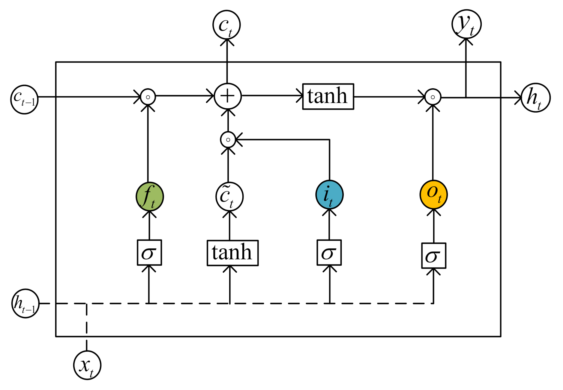
Compared with ordinary RNN, LSTM neural network is also composed of an input layer, output layer, and hidden layer, but its hidden layer is replaced by ordinary neurons with memory modules containing gating mechanism. Its internal structure is shown in the Figure 1.

The memory unit c_t is the core component of the LSTM memory module. It is realized by controlling the forget gate, input gate, and output gate. It contains the long-term memory information of the sequence. The hidden layer state h_t contains the short-term memory information of the sequence, which is updated faster than memory unit update speed [16].

Suppose a total of k time steps of the input vector sequence are divided into x₁, x₂, ..., x_k according to the input time sequence, and the t-th time step is taken for analysis.

The LSTM operation rules are as follows:

(1) Update the output of the forget gate, select the historical information that the memory unit needs to keep, and control the degree of influence of c_t−1 on c_t:

$$f_t=\sigma (W_f{x}_t+U_f{h}_{t-1}+b_f)$$

(8)

(2) Update the two parts of the output of the input gate, select the current input information that the memory unit needs to retain, and control the degree of influence of x_t on c_t:

$$f_t=\sigma (W_f{x}_t+U_f{h}_{t-1}+b_f)$$

(9)

$${\tilde{c}}_t=\tanh (W_c{x}_t+U_c{h}_{t-1}+b_c)$$

(10)

(3) Update the cell status according to the input gate and forget gate:

$$c_t=f_t\circ c_{t-1}+i_t\circ c_t\prime$$

(11)

(4) Update the output gate output, select the output information that the memory unit needs to retain, and control the degree of influence of c_t on h_t:

$$o_t=\sigma (W_o{x}_t+U_o{h}_{t-1}+b_o)$$

(12)

$$h_t=o_t\circ \tanh (c_t)$$

(13)

(5) Update the forecast output at the current moment:

$${\widehat{y}}_t=\sigma \left(V{h}_t+c\right)$$

(14)

Among them, f_t, i_t, and o_t represent the calculation results of the forget gate, input gate, and output gate at time t; W_f, Wi, and Wo represent the weight matrix of the forget gate, input gate, and output gate, respectively; b_f, b_i, and b_o represent the weight matrix of the forget gate, input gate, and output gate, respectively. The bias term of the forget gate, input gate, and output gate; o is the dot product symbol of the matrix element; σ(x) is the Sigmoid activation function of each gate:

$$\sigma \left(x\right)=\frac{1}{1+e^{-1}}$$

(15)

Its value range is (0, 1). Through the conversion of Sigmoid function, the input can be converted into probability values, so it is widely used as the activation function of artificial neural network transmission.

When x_t is input to the network, it will be processed by a tanh neural layer and three gates at the same time as the hidden layer vector h_t−1 of the previous time step. The tanh function is a hyperbolic tangent activation function, and its expression is:

$$\tanh \left(x\right)=\frac{\sinh \left(x\right)}{\cosh \left(x\right)}=\frac{e^{2x}-1}{e^{2x}+1}$$

(16)

Its value range is (−1, 1), the output is centered at the origin, and the convergence speed is faster than that of Sigmoid. It is usually used as the activation function of the output gate.

The tanh layer will create a new candidate state vector c_t′. The forgetting gate f_t determines what information to discard and retain from the cell state c_t−1 of the previous time step. The input gate it determines how to update the candidate state vector. After the cell state is updated, the output gate o_t decides how to filter the new state vector c_t into output information h_t.

2.2.2. Training Process of LSTM

The training algorithm of LSTM neural network mainly includes two categories: back propagation algorithm over time and real-time cyclic learning algorithm. The concept of backpropagation algorithm is clear and it has advantages in computational efficiency. This paper selects this method to train LSTM neural network.

The back propagation method expands the LSTM into a deep feedforward neural network in time sequence, and then further calculates the relevant parameter gradients according to the error back propagation algorithm of the feedforward network, and trains the model [18]. The LSTM network sequence expansion diagram is shown in Figure 2.

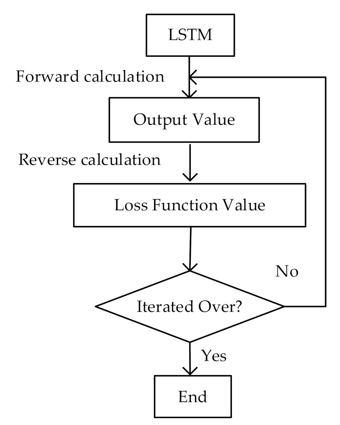
The specific training steps are as follows in Figure 3.

(1) Forward calculation of the output value of the LSTM memory module.

The c_t and h_t of the current time step are calculated by the gating mechanism of LSTM and are retained for the calculation of the next time step. When the calculation of the last step is completed, the hidden layer vector h_k will be used as the output and the prediction corresponding to this set of sequences’ value (tag value) to compare.

(2) Reverse calculation of the error item value of each memory module, including two reverse propagation directions in chronological order and at network level.

Calculate the loss function value according to the comparison result of step 1, and select the square sum error function as the loss function of LSTM; the expression is:

$$L=\frac{1}{2}{\displaystyle \sum _{i\in outputs}{\left({\widehat{y}}_i-y_i\right)}^2}$$

(17)

(3) According to the corresponding error term, calculate the gradient of each weight, and the gradient descent method iterates the parameters including W, U, V, c_t, and h_t:

$${\widehat{\theta }}_j={\theta }_j-\alpha \frac{\partial }{\partial {\theta }_j}L\left({\theta }_j\right)$$

(18)

Through the gating mechanism and perfect parameter update rules, LSTM realizes the selection and screening of the input information flow, and improves the processing ability of the recurrent neural network for long sequences.

The back-propagation algorithm can compare the predicted value with the real value by using the error function after the forward calculation, and then optimize the network parameters. Therefore, the back-propagation algorithm can back calculate and optimize many parameters of LSTM. The cyclic learning algorithm can deal with some sequence problems, but it has serious long-term dependence problems after multi-stage propagation—the gradient tends to disappear or explode, and it is difficult to continue to optimize within the number of iterations in many cases. However, the introduction of gating mechanism in LSTM solves the gradient disappearance problem and performs well in sequence processing.

2.2.3. Bidirectional LSTM

The bidirectional long and short-term memory (Bi-LSTM) network is derived from the bidirectional cyclic neural network [19]. Its main feature is to increase the learning function of the neural network for future information, thereby overcoming the defect that the unidirectional LSTM network can only process historical information. The Bi-LSTM mainly splits the ordinary LSTM into two directions, but the two LSTMs are connected to the same output layer. Such a structure can provide complete upper and lower sequence information for the input sequence of the output layer. Using a Bi-LSTM network to model bus load forecasting is to input historical data into a forward LSTM network and a reverse LSTM network at the same time, so as to capture a complete time series global information. The Bi-LSTM neural network structure diagram is as follows in Figure 4.

Because the bus load has certain regularity and planning, the joint grasp of historical and future information can better learn the characteristics and laws of the load curve.

The update formula of the back-to-forward cycle neural network layer is:

$$h_{1,t}=f\left(W_{h_1,t}{x}_t+W_{h_1}{h}_{1,t-1}+b_{h_1}\right)$$

(19)

The update formula of the looping neural network layer from front to back is:

$$h_{2,t}=f\left(W_{h_2,t}{x}_t+W_{h_2}{h}_{2,t+1}+b_{h_2}\right)$$

(20)

The two layers of recurrent neural networks are superimposed and input to the hidden layer:

$$y_t=g\left(U_{h_1}{h}_{1,t}+U_{h_2}{h}_{2,t}+b_y\right)$$

(21)

Among them, h₁, t, and h₂, t are the hidden units of the front pass layer and the back pass layer at time t, respectively; y_t is the model output at time t; f(*), g(*) are optional activation functions; W_h1,t, W_h2, t, W_h1, W_h2, U_h1, and U_h2 are the weight matrices of the corresponding objects; and b_h1, b_h2, and b_y are the bias terms of the corresponding objects.

2.3. Bayesian Optimization of LSTM

2.3.1. Bayesian Optimization Theory

Gaussian Regression Process

In the feasible region, uniformly select points that obey the multi-dimensional normal distribution as candidate solutions to establish a Gaussian regression model [20]:

$$\left[\begin{array}{c}{y}_1\\ ⋮\\ y_n\end{array}\right]\sim N\left(0,\left[\begin{array}{ccc}k\left(x_1,x_1\right)& \cdots & k\left(x_1,x_n\right)\\ ⋮& & ⋮\\ k\left(x_n,x_1\right)& \cdots & k\left(x_n,x_n\right)\end{array}\right]\right)$$

(22)

Among them, K is the covariance matrix, x is the input value, and y is the response output value.

Through the training set, the updated value y* is obtained according to the posterior formula:

$$P\left(y_{\ast }\left|y\sim N\left(K_{\ast }{K}^{-1}y,K_{\ast \ast }-K^{-1}{K}_{\ast }^T\right)\right.\right)$$

(23)

Among them, K_∗ is the covariance of the training set, and K_∗∗ is the covariance of the newly added sample.

Update the Gaussian regression model according to the updated value:

$$\left[\begin{array}{c}y\\ y_{\ast }\end{array}\right]\sim N\left(0,\left[\begin{array}{cc}K& K_{\ast }^T\\ K_{\ast }& K_{\ast \ast }\end{array}\right]\right)$$

(24)

The Gaussian regression model considers the relationship between y_N and y_N+1 and establishes input and output functions to provide a search basis for parameter optimization.

Acquisition Function Process

On the basis of the Gaussian regression model, it is necessary to use the collection function to solve the optimal solution of the function. This paper selects the expectation improvement method to use the mathematical expectation to solve the optimal solution.

$$x_{n+1}=\arg \max E{I}_n\left(x\right)$$

(25)

$$E{I}_n\left(x\right)=E_n\left[{\left[f\left(x\right)-f_n^{\ast }\right]}^{+}\right]$$

(26)

$$=\left(\mu -f_n^{\ast }\right)\left(1-\varphi \left(\frac{f_n^{\ast }-\mu }{\sigma }\right)\right)+\sigma \phi \left(\frac{f_n^{\ast }-\mu }{\sigma }\right)$$

(27)

Among them, ϕ(x) is the probability density of the normal distribution, φ(x) is the standard normal distribution about x, μ is the mean value of the input value x, and σ is the variance of the input value x.

The expected value is used for parameter optimization, and the next optimal value is effectively sought within a certain range, so as to find the optimal parameter within the number of iterations [20].

2.3.2. Hyperparameter Optimization of LSTM

The hyperparameters of the LSTM neural network used for bus load prediction can be divided into two categories: structural hyperparameters and training hyperparameters. The structural hyperparameters mainly include the number of hidden neurons in the network, etc [21]. The number of hidden layer neurons determines the expressive ability of the network, but also determines whether the network is over-fitting and the network is time-consuming. Reasonable hidden layer neurons help improve the performance of the network’s predictive ability. The use of the bidirectional long-term memory network improves the network’s ability to learn historical data, but it also leads to slow network prediction and different effects. Choosing different curves to predict whether to use a Bi-LSTM can save prediction time while ensuring prediction accuracy [22].

The training hyperparameters of the LSTM neural network mainly include learning rate, L2 regularization parameters, etc. A suitable initial learning rate helps to significantly improve the iterative convergence speed and prediction accuracy of deep learning models. L2 regularization parameters are additional items of the network loss function and can prevent the over-fitting problem to a certain extent.

In summary, this paper will use Bayesian optimization algorithm to optimize and debug the number of hidden layer neurons of LSTM neural network, whether to use Bi-LSTM, initial learning rate, and L2 regularization parameters.

2.4. VMD-Bi-LSTM Combined Prediction Model

The power system bus load itself has fluctuating characteristics and is affected by distributed power dispatch and user-side behavior characteristics. Its curve has a certain degree of non-linear and non-stationary characteristics. The use of conventional learning forecasting methods to improve the forecasting accuracy is relatively limited. Considering the outstanding advantages of variational modal decomposition technology in sequence smoothing processing and the excellent performance of LSTM networks in time series data modeling, this paper proposes a VMD-Bi-LSTM combined forecasting model. The specific modeling process is as follows, as shown in the Figure 5.

(1) In view of the non-stationary characteristics of the bus load sequence, the VMD method is used to decompose, and each IMF component and residual component are obtained;

(2) Normalize each sub-sequence component separately, and divide the training sample and the test sample according to the same ratio;

(3) Construct an LSTM neural network prediction model for each sub-sequence component, and use Bayesian optimization algorithm to optimize the hyperparameters of a single model to obtain the most suitable hyperparameter combination for decomposing the sequence and determine whether to use Bi-LSTM in sub-sequences;

(4) Train the prediction model after hyperparameter optimization, use the trained prediction model to perform multi-step extension prediction, and superimpose the reconstruction to obtain the multi-step prediction value of bus load;

(5) Compared with actual data, the multi-step prediction performance of the prediction model is evaluated by calculating error indicators.

3. Case Study

Here, we analyze the example of the method proposed in this paper. The example takes the bus load data of Canberra, Australia, from 16 January to 22 January 2016 as the data set, including 270 time steps (30 min as a time step). The first 244 time steps of the data are used as the training sequence and the last 36 time steps are used as the verification sequence.

3.1. Temporal Data Decomposition

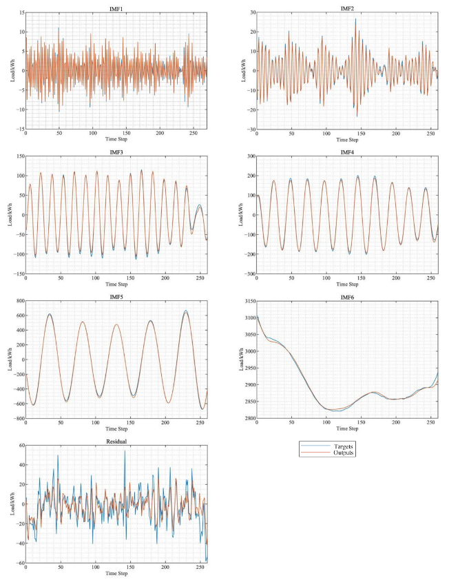
The original bus load sequence is decomposed byVMD, and six groups of IMF components and one group of residual components are separated step by step. The decomposition results are shown in Figure 6.

Decomposing the bus load sequence through variational modal decomposition shows that the natural modal function consists of multiple sub-sequences with small amplitude and stable frequency. Although the frequency of the remainder is relatively unstable, the amplitude is small, which affects the overall bus load. The forecast trend change of the load has less impact.

3.2. Hyperparameter Optinization of VMD-LSTM

On the basis of smoothing the original sequence, it is necessary to construct the LSTM network prediction model of the sub-sequence components, and to optimize the related structure hyperparameters and training hyperparameters. The hyperparameter results obtained by using Bayesian optimization algorithm in this paper are shown in the

Table 1. Hyperparameters of each subsequence.

Sequence	Number of Units	Using Bi-LSTM Layer	Initial Learning Rate	L2 Regularization
IMF 1	197	1	0.01	0.0013
IMF 2	73	2	0.011	0.00018
IMF 3	66	1	0.011	0.000021
IMF 4	64	2	0.016	0.0024
IMF 5	199	1	0.01	1.16
IMF 6	140	1	0.021	0.00018
Residual	130	1	0.01	0.00097

.

3.3. Model Evaluation Index

In order to visually analyze the predicted error value, the curve correlation coefficient is introduced to evaluate the shape difference between the predicted curve and the real curve, and the root mean square error (RMSE) is introduced to visually analyze the deviation between the observed value and the true value. The accuracy is analyzed, and the standard error is selected as the criterion for predicting the dispersion level.

In order to evaluate the forecasting effect of the proposed bus load forecasting method, the RMSE, NRMSE, standard error, and correlation coefficient are selected as the overall forecasting results evaluation index of the short-term bus load forecasting method.

$$e_{RMSE}=\sqrt{\frac{1}{n}{{\displaystyle \sum _{i=1}^n\left(y_i-{\widehat{y}}_i\right)}}^2}$$

(28)

$$e_{NRMSE}=\sqrt{\frac{RMSE}{mean\left({\displaystyle \sum _{i=1}^n{y}_i}\right)}}$$

(29)

$$e_{STD}=\sqrt{\frac{{\displaystyle \sum _{i=1}^n{\left(y_i-{\widehat{y}}_i\right)}^2}}{n}}$$

(30)

$$\rho \left(A,B\right)=\frac{1}{N-1}{\displaystyle \sum _{i=1}^N\left(\frac{\overline{A_i-{\mu }_A}}{{\sigma }_A}\right)\left(\frac{B_i-{\mu }_B}{{\sigma }_B}\right)}$$

(31)

where σ_A and σ_B are the standard deviation of dataset A and dataset B, respectively, and the standard deviation formula is as follows:

$${\sigma }_x=\sqrt{\frac{{\displaystyle \sum _{i=1}^n{\left(x_i-\overline{x}\right)}^2}}{n-1}}$$

(32)

where y_i is the true value of bus load and ${\widehat{y}}_i$ is the predicted value of bus load. The correlation coefficient r is used to characterize the accuracy of the prediction curve and the calibration curve. The closer the correlation coefficient is to 1, the higher the prediction accuracy.

3.4. Model Evaluation Index

After optimizing the Bayesian parameters of each sub-sequence of the bus load, the long and short-term memory network is trained, and the next time step is predicted in Figure 7, and the single-step prediction results of each sub-sequence component are integrated into the historical monitoring data. The new input sequence of the single-step forecasting model can realize the multi-step rolling forecast of each component, which can realize the rolling forecast load value for a period of time in the future. The rolling prediction method is used to predict multiple time steps in the future, and the prediction results are shown in Figure 8.

The multi-step prediction results of bus load can be obtained by superimposing the predicted values of each subsequence, and the error analysis of each subsequence is carried out by using the prediction evaluation index. The error results are shown in

Table 2. Performance comparison of multi-step prediction.

Sequence	Time Step	eRMSE	r	eNRMSE	eSTD
IMF 1	12	0.8909	0.9917	7.6779	0.9299
	24	0.7262	0.9904	−39.3426	0.7265
	36	0.6631	0.9899	−33.9655	0.6387
IMF 2	12	1.1507	0.9941	−0.7562	1.0931
	24	1.1929	0.9877	−2.3908	1.2184
	36	1.1635	0.9834	−2.5087	1.1713
IMF 3	12	7.9527	0.9904	−0.5446	2.9920
	24	6.7540	0.9882	−0.7751	4.2085
	36	7.7266	0.9840	−4.8082	7.6166
IMF 4	12	5.0755	0.9999	0.0630	1.5155
	24	8.7905	0.9987	2.8258	5.2502
	36	14.6416	0.9869	2.2186	14.6664
IMF 5	12	15.7076	0.9999	0.2571	8.4288
	24	15.2865	0.9997	−0.0559	9.7277
	36	15.3647	0.9996	−0.0740	10.4295
IMF 6	12	1.3635	0.9521	0.000472	0.8233
	24	7.6753	0.9585	0.0026	5.9782
	36	20.2677	0.992	0.0069	14.6026
Residual	12	11.4701	0.6938	9.4522	11.9700
	24	17.4227	0.6755	−1.5639	15.2513
	36	15.9639	0.6827	−1.3800	15.3315

. From the training prediction results and multi-step prediction results, it can be seen that the e_RMSE of IMF6, which accounts for a large proportion of the original sequence of bus load, is 1.3635 and e_STD is 0.8233 in the next 12 time steps, with small prediction error. With the increase in prediction time steps, the prediction e_RMSE in the next 36 time steps will increase to 20.2677, e_STD and e_NRMSE will also increase accordingly, but the r will increase from 0.9521 to 0.992. The shape of the prediction curve will gradually stabilize and be closer to the shape of the original curve. With the increase in time steps, the prediction accuracy will decline, but the prediction curve will gradually remain stable; the shape gradually approaches the original curve, which has suitable prediction stability.

The prediction e_NRMSE of other subsequences is lower than 16, the r is higher than 0.98, the prediction error is small, and the prediction shape remains suitable. The prediction results of a single stable natural mode function subsequence meet expectations.

The decomposition remainder of bus load has many burrs and unstable frequency, so the prediction correlation coefficient is low. However, due to its small amplitude, its prediction error is also small, and its impact on the overall prediction result of bus load is relatively small.

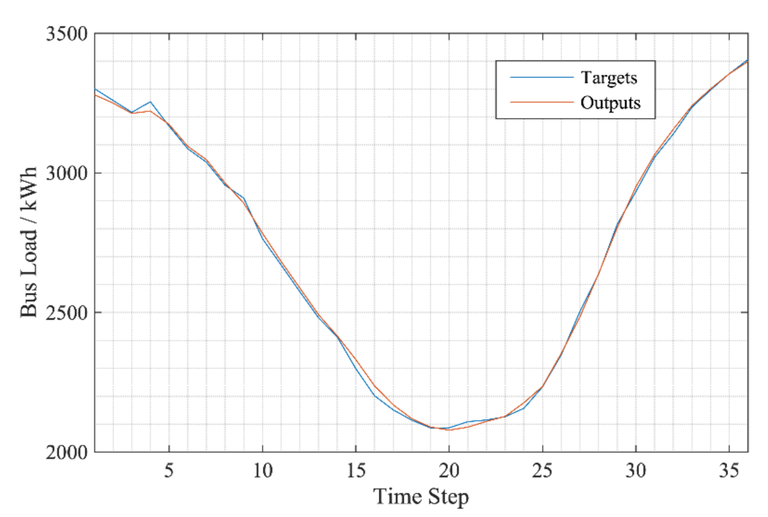
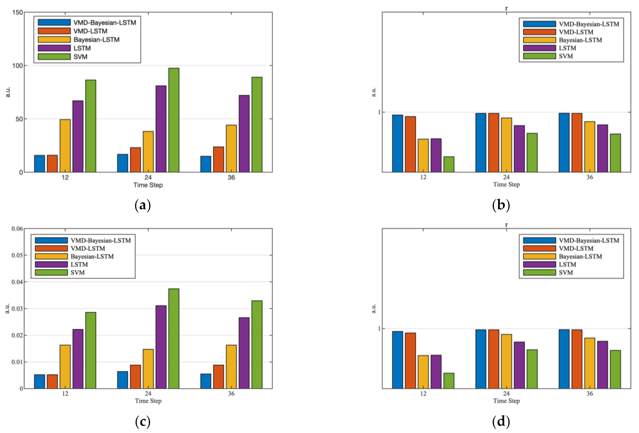
The multi-step prediction results of each subsequence and remainder are superimposed to obtain the multi-step prediction curve of bus load, as shown in Figure 9. The prediction curve fits with the real curve and has accurate prediction results. In order to verify the prediction performance of the proposed method, different models in various cases are selected for comparative analysis. The SVM that uses radial basis function as kernel function for prediction is compared with LSTM to verify the advantages of LSTM in time series prediction. The VMD-Bayesian-BiLSTM model is compared with EEMD-Bayesian-BiLSTM model and EMD-Bayesian-BiLSTM to verify the advantages of VMD in short-term combination forecasting. The VMD-LSTM combined prediction model and LSTM model are selected for prediction to verify the prediction accuracy and stability of the combined prediction model. The VMD-Bayesian-LSTM model is compared with VMD-LSTM model, and the Bayesian-BiLSTM model is compared with the Bayesian-LSTM model and LSTM to verify the improvement effect of Bayesian optimization theory on LSTM prediction accuracy and the necessity to consider the applicability of BiLSTM in sequence prediction. The comparison results are shown in

Table 3. Performance comparison of different models.

Title 1	Time Step	eRMSE	r	eNRMSE	eSTD
VMD-Bayesian-BiLSTM	12	15.7524	0.9986	0.0052	16.4296
	24	16.6947	0.9994	0.0064	16.6392
	36	14.9219	0.9995	0.0055	14.8022
EEMD-Bayesian-BiLSTM	12	19.6386	0.9963	0.0073	16.4825
	24	22.3739	0.9971	0.0088	17.9276
	36	26.8462	0.9951	0.0091	21.9372
EMD-Bayesian-BiLSTM	12	21.8372	0.9968	0.0083	17.8362
	24	25.8376	0.9946	0.0096	19.8372
	36	28.3826	0.9938	0.0105	23.8261
VMD-BiLSTM	12	15.8235	0.9978	0.0052	16.4784
	24	22.9478	0.9974	0.0073	20.4936
	36	23.7018	0.9968	0.0088	20.9806
Bayesian-BiLSTM	12	25.6357	0.9965	0.0092	21.9365
	24	30.6387	0.9956	0.0105	25.3794
	36	32.7487	0.9947	0.0124	28.3748
Bayesian-LSTM	12	49.3128	0.9865	0.0163	43.5910
	24	38.2263	0.9971	0.0147	35.6199
	36	44.1296	0.9953	0.0163	44.7550
LSTM	12	66.9500	0.9867	0.0222	40.1171
	24	80.9277	0.9933	0.0311	53.9405
	36	71.9871	0.9937	0.0266	55.8161
SVM	12	86.4025	0.9777	0.0286	51.8872
	24	97.3993	0.9894	0.0374	67.1863
	36	89.0407	0.9891	0.0329	71.4600

and Figure 10.

The comparison of different models shows that the prediction accuracy of each time step of LSTM is greatly improved compared with SVM. After decomposing the bus load sequence, the e_RMSE, r and other indices of VMD-LSTM are greatly improved on the basis of the LSTM model, which greatly improves the prediction accuracy and stability. The comparison of VMD-Bayesian-BiLSTM and EEMD-Bayesian-BiLSTM and the comparison of VMD-Bayesian-BiLSTM and EMD-Bayesian-BiLSTM shows that the prediction error of the prediction model considering VMD in multiple time steps is lower than that of EMD and EEMD. With the proposal of Bayesian optimization theory, the e_RMSE of 36 time steps of combined prediction is reduced from 23.9219 to 14.9219, the e_NRMSE is reduced from 0.0088 to 0.0055, the e_STD is reduced from 20.9806 to 14.8022, and the results of LSTM are also greatly improved after Bayesian optimization. The results of the Bayesian-BiLSTM model are improved compared with those without considering Bi-LSTM. The comparison of various data shown in Figure 10 verifies that the VMD-LSTM combined prediction model based on Bayesian optimization proposed in this paper has more accurate prediction results and more stable multi-step prediction results.

In order to verify the applicability of the model proposed in this paper, this paper randomly selects two groups of 270 time step data sets in the bus load data set in Canberra, Australia, in 2016, which are divided into data set 2 and data set 3 for verification. In order to eliminate the regional influence, three groups of 270 time step data sets are randomly selected from the 2014 Beijing bus load data set, namely data set 4, data set 5, and data set 6, and their errors are tested in

Table 4. Test of different data sets.

Title 1	Time Step	eRMSE	r	eNRMSE	eSTD
Data set 1	12	15.7524	0.9986	0.0052	16.4296
	24	16.6947	0.9994	0.0064	16.6392
	36	14.9219	0.9995	0.0055	14.8022
Data set 2	12	16.8362	0.9993	0.0058	16.4784
	24	17.9378	0.9987	0.0078	17.9387
	36	17.9373	0.9989	0.0083	17.9272
Data set 3	12	15.9327	0.9991	0.0055	16.9365
	24	16.9372	0.9989	0.0067	18.3794
	36	18.8372	0.9988	0.0093	19.3748
Data set 4	12	17.3128	0.9995	0.0163	18.5910
	24	18.2263	0.9988	0.0147	19.6199
	36	19.1296	0.9985	0.0163	21.7550
Data set 5	12	17.8362	0.9993	0.0087	18.8362
	24	19.8367	0.9983	0.0093	20.9837
	36	21.8272	0.9969	0.0128	22.9472
Data set 6	12	18.8367	0.9991	0.0115	19.8362
	24	18.9272	0.9992	0.0134	20.9372
	36	20.8367	0.9983	0.0176	21.9272
Average Value	12	17.0845	0.9992	0.0088	17.8513
	24	18.0933	0.9989	0.0097	19.0830
	36	18.9149	0.9985	0.0116	19.7889

.

It can be seen from Table 4 that through the test of multiple groups of randomly selected data in the same time step, the error value is always controlled in a low range, and the average error of six groups of data has suitable prediction results. This shows that the proposed method has appropriate prediction stability and adaptability.

4. Conclusions and Future Studies

Aiming at the current research hotspot in the field of deep learning, this paper studies the bus load forecasting, establishes the bus load forecasting method based on VMD-BiLSTM, and draws the following conclusions:

(1) The VMD method is used to deal with the non-stationary characteristics of bus load series and reduce the interaction between different time scale information, which is conducive to further mining the characteristics of original series and improving the prediction performance of the model;

(2) The cyclic network structure and gating mechanism of LSTM neural network are used to capture the temporal correlation of each sub sequence component, so as to track the change trend of bus load more effectively. Compared with other models, the VMD-LSTM combined prediction model has a significant improvement in multi-step prediction accuracy;

(3) Bayesian optimization algorithm is used to optimize the super parameter combination of LSTM neural network to overcome the adverse effect of empirical selection on the improvement of model prediction performance;

(4) Bayesian optimization considers the applicability of the sequence to the bidirectional neural network. While using the Bi-LSTM network to enhance the training ability, considering the applicability of the sequence, the prediction performance of the network has been optimized and improved.

This method has certain feasibility in the field of bus load forecasting, can be applied in the direction of energy consumption forecasting and power production planning, and is conducive to the planning and development of clean energy in the future and the sustainable development of energy.

The model proposed in this paper has achieved suitable results in short-term prediction, but it is uncertain whether it can ensure the prediction accuracy and stability in long-term prediction when the data support is sufficient, and whether it is adaptable in other areas. Due to time constraints, this paper does not compare it with ETS, ARIMA, and Thet to reflect the optimization performance. In the future, this proposed model can be implemented in different areas to validate its effectiveness and compared to alternative approaches and stronger baselines. Moreover, by taking a new variety of data input for sustainability studies, the model can be implemented for carbon emission forecasting. The author will study and optimize the excellent prediction methods in the field of machine learning in order to establish an accurate prediction model that can be applied in the field of sustainability.

References

- Deutsch, J.; He, D. Using Deep Learning-Based Approach to Predict Remaining Useful Life of Rotating Components. IEEE Trans. Syst. Man Cybern. Syst. 2017, 48, 11–20. [Google Scholar] [CrossRef]
- Zhao, P.; Dai, Y. Power load forecasting of SVM based on real-time price and weighted grey relational projection algorithm. Power Syst. Technol. 2020, 44, 1325–1332. [Google Scholar]
- Zang, H.; Xu, R.; Cheng, L.; Ding, T.; Liu, L.; Wei, Z.; Sun, G. Residential load forecasting based on LSTM fusing self-attention mechanism with pooling. Energy 2021, 229, 120682. [Google Scholar] [CrossRef]
- Memarzadeh, G.; Keynia, F. Short-term electricity load and price forecasting by a new optimal LSTM-NN based prediction algorithm. Electr. Power Syst. Res. 2020, 192, 106995. [Google Scholar] [CrossRef]
- Ning, J.; Hao, S.; Zeng, A.; Chen, B.; Tang, Y. Research on Multi-Timescale Coordinated Method for Source-Grid-Load with Uncertain Renewable Energy Considering Demand Response. Sustainability 2021, 13, 3400. [Google Scholar] [CrossRef]
- Salinas, D.; Flunkert, V.; Gasthaus, J.; Januschowski, T. DeepAR: Probabilistic forecasting with autoregressive recurrent networks. Int. J. Forecast. 2019, 36, 1181–1191. [Google Scholar] [CrossRef]
- Oreshkin, B.N.; Carpov, D.; Chapados, N.; Bengio, Y. N-BEATS: Neural Basis Expansion Analysis for Interpretable Time Series Forecasting. In Proceedings of the ICLR 2020, Addis Ababa, Ethiopia, 30 April 2020. [Google Scholar]
- Li, S.; Jin, X.; Xuan, Y.; Zhou, X.; Chen, W.; Wang, Y.; Yan, X. Enhancing the Locality and Breaking the Memory Bottleneck of Transformer on Time Series Forecasting. In Proceedings of the NeurlPS 2019, Vancouver, Canada, 8–14 December 2019. [Google Scholar]
- Zheng, J.; Su, M.; Ying, W.; Tong, J.; Pan, Z. Improved uniform phase empirical mode decomposition and its application in machinery fault diagnosis. Measurement 2021, 179, 109425. [Google Scholar] [CrossRef]
- Wang, J.; Athanasopoulos, G.J.; Hyndman, R.; Wang, S. Crude oil price forecasting based on internet concern using an extreme learning machine. Int. J. Forecast. 2018, 34, 665–677. [Google Scholar] [CrossRef]
- Lin, G.; Lin, A.; Cao, J. Multidimensional KNN algorithm based on EEMD and complexity measures in financial time series forecasting. Expert Syst. Appl. 2021, 168, 114443. [Google Scholar] [CrossRef]
- Zhang, Z.; Hong, W. Application of variational mode decomposition and chaotic grey wolf optimizer with support vector regression for forecasting electric loads. Knowl. Based Syst. 2021, 228, 107297. [Google Scholar] [CrossRef]
- Zhu, Q.; Zhang, F.; Liu, S.; Wu, Y.; Wang, L. A hybrid VMD–BiGRU model for rubber futures time series forecasting. Appl. Soft Comput. 2019, 84, 105739. [Google Scholar] [CrossRef]
- Liu, Y.; Xu, Z.; Dong, W.; Li, Z.; Gao, S. Concentration prediction of dissolved gases in transformer oil based on empirical mode decomposition and long short-term memory neural networks. J. Chin. Electr. Eng. Sci. 2019, 39, 3998–4008. [Google Scholar]
- Wang, C.; Yue, S.; Wei, S.; Lv, J. Performance analysis of four decomposition-ensemble models for one-day-ahead agricultural commodity futures price forecasting. Algorithms. 2017, 10, 108. [Google Scholar] [CrossRef]
- Zhao, Y.; Wang, X.; Jiang, C.; Zhang, J.; Zhou, Z. A novel short-term electricity price forecasting method based on correlation analysis with the maximal information coefficient and modified multi-hierachy gated LSTM. J. Chin. Electr. Eng. Sci. 2021, 41, 135–146. [Google Scholar]
- Zhen, H.; Niu, D.; Yu, M.; Wang, K.; Liang, Y.; Xu, X. A Hybrid Deep Learning Model and Comparison for Wind Power Forecasting Considering Temporal-Spatial Feature Extraction. Sustainability 2020, 12, 9490. [Google Scholar] [CrossRef]
- Kraft, E.; Keles, D.; Fichtner, W. Modeling of frequency containment reserve prices with econometrics and artificial intelligence. J. Forecast. 2020, 39, 1179–1197. [Google Scholar] [CrossRef] [Green Version]
- Mughees, N.; Mohsin, S.; Mughees, A.; Mughees, A. Deep sequence to sequence Bi-LSTM neural networks for day-ahead peak load forecasting. Expert Syst. Appl. 2021, 175, 0957–4174. [Google Scholar] [CrossRef]
- Han, Y.; Lam, J.C.; Li, V.O.; Reiner, D. A Bayesian LSTM model to evaluate the effects of air pollution control regulations in Beijing, China. Environ. Sci. Policy 2020, 115, 26–34. [Google Scholar] [CrossRef]
- Jamilloux, Y.; Romain-Scelle, N.; Rabilloud, M.; Morel, C.; Kodjikian, L.; Maucort-Boulch, D.; Bielefeld, P.; Sève, P. Development and Validation of a Bayesian Network for Supporting the Etiological Diagnosis of Uveitis. J. Clin. Med. 2021, 10, 3398. [Google Scholar] [CrossRef] [PubMed]
- Wu, K.; Wu, J.; Feng, L.; Yang, B.; Liang, R.; Yang, S.; Zhao, R. An attention-based CNN-LSTM-BiLSTM model for short-term electric load forecasting in integrated energy system. Int. Trans. Electr. Energy Syst. 2021, 31, e12637. [Google Scholar] [CrossRef]
Figure 1.
Internal structure of LSTM.
Figure 2.
Sequence structure diagram of LSTM.
Figure 3.
Training steps of LSTM.
Figure 4.
Bi-LSTM Neural Network Structure Diagram.
Figure 5.
Flowchart of VMD-BiLSTM combined prediction.
Figure 6.
(a) Original sequence and IMFs; (b) IMFs and residual.
Figure 7.
Subsequence training prediction results.
Figure 8.
Subsequence multi-step prediction results.
Figure 9.
Prediction results of VMD-BiLSTM.
Figure 10.
(a) Comparison of eRMSE; (b) comparison of r; (c) comparison of eNRMSE; (d) comparison of eSTD.