Absolute Contribution of the Non-Uniform Spatial Distribution of Atmospheric CO₂ to Net Primary Production through CO₂-Radiative Forcing

Abstract

Atmospheric concentrations of CO₂ are the most important driver of the Earth’s climate and ecosystems through CO₂-radiative forcing, fueling the surface temperature and latent heat flux on half-century timescales. We used FGOALS-s2 coupled with AVIM2 to estimate the response of net primary production (NPP) to spatial variations in CO₂ during the time period 1956–2005. We investigated how the induced variations in surface temperature and soil moisture influence NPP and the feedback of the oceans and sea ice on changes in NPP. The spatial variations in the concentrations of CO₂ resulted in a decrease in NPP from 1956 to 2005 when we included ocean and sea ice dynamics, but a slight increase in NPP without ocean and sea ice dynamics. One of the reasons is that the positive feedback of sea temperature to the surface temperature leads to a significant decrease in tropical NPP. Globally, the non-uniform spatial distribution of CO₂ absolutely contributed about 14.3% ± 2.2% to the terrestrial NPP when we included ocean and sea ice dynamics or about 11.5% ± 1.1% without ocean and sea ice dynamics. Our findings suggest that more attention should be paid to the response of NPP to spatial variations in atmospheric CO₂ through CO₂-radiative forcing, particularly at low latitudes, to better constrain the predicted carbon flux under current and future conditions. We also highlight the fundamental importance of changes in soil moisture in determining the pattern, response and magnitude of NPP to the non-uniform spatial distribution of CO₂ under a warming climate.

1. Introduction

Atmospheric CO₂ concentrations are one of the most important drivers of climate in earth system models [1,2]. It can affect the global average surface temperature, the global water cycle, global sea-levels, the loss of Arctic sea ice and the atmospheric vapor pressure deficit through radiative forcing [3,4,5]. Changes in CO₂ concentrations indirectly affect the growth of land plants and the productivity of terrestrial vegetation (gross primary production) [6]—for example, the gross primary production of terrestrial vegetation decreased after the late 1990s as a result of the increased vapor pressure deficit [5].

There is large uncertainty in the magnitude and spatial distribution of the radiative effect of atmospheric CO₂ concentration (±20%) based on multi-model simulations [7,8]. These models come from the fifth stage of the coupled model comparison project (CMIP5) [9] using the uniformity of atmospheric CO₂ concentration without spatial varying. Although the spatial heterogeneity of atmospheric CO₂ concentrations varies widely on a regional scale [10,11], the contribution of spatially non-uniform CO₂ to the Earth’s climate and the terrestrial carbon cycle through CO₂-radiative forcing is largely unknown [12].

Several studies have reported the impacts of varying atmospheric CO₂ concentrations directly through CO₂-radiative forcing on climate state [13,14]. Furthermore, it can also disturb the carbon balance [15] and accumulation of carbon on land [16]. For instance, the variations in surface temperature, precipitation and soil moisture [17] influence the rate of photosynthesis and limit net primary production (NPP) and soil respiration [15]. Thus, changes in the Earth’s climate through CO₂-radiative forcing therefore constrain the processes of the carbon cycle [2].

However, predictions of the rise in temperature under historical conditions remain highly uncertain, ranging from about 0.4 to 1.3 °C, mainly due to historical radiative forcing of greenhouse gases [18]. One of the uncertainties results from the lack of a clear understanding about the feedback of spatial variations in atmospheric CO₂ and the lack of reliable measurements of this process in the field. Modeling approaches are therefore vital to constrain climate variables and the carbon fluxes resulting from the spatial varying of CO₂ concentration.

On the other hand, most conventional methodologies do not consider the influence of spatial varying of CO₂ concentrations on the Earth’s climate system and biogeochemical cycles. We would focus to quantify the response of terrestrial NPP to the spatial varying of CO₂ concentration through CO₂-radiative forcing. To further assess the significance of the non-uniform spatial distribution of CO₂ on NPP, we compared simulations with fully coupled atmosphere–land–ocean–sea ice components (simulation A) and coupled atmosphere–land components (simulation B) in the Flexible Global Ocean–Atmosphere–Land System Model Spectral Version 2 (FGOALS-s2) [19] coupled with the Atmosphere–Vegetation Interaction Model (AVIM) [20]. Specifically, we evaluated NPP in FGOALS-AVIM with the implementation of these two different simulations forced by a uniform or non-uniform spatial distribution of atmospheric CO₂ with or without active ocean and sea ice during the time period 1956–2005. We addressed three principal questions: (1) how much does the climate-driven feedback caused by the non-uniform spatial distribution of CO₂ through CO₂-raiative forcing affect climate variables and NPP; (2) how does the estimated NPP with and without ocean and sea ice dynamics differ as a result of the non-uniform spatial distribution of CO₂ through the radiative forcing associated with spatial variations in the climate variables; and (3) what are the implications of a non-uniform spatial distribution of CO₂ on the global NPP during the time period 1956–2005.

2. Methods and Simulations

The Student’s t-test used in this study is used to estimate of the statistical significance between the variables from different simulations, which are calculated as follows:

$${\mathrm{t}}_{\mathrm{i}}=\frac{ \overline{{\mathrm{x}}_{\mathrm{i}}}-\overline{{\mathrm{y}}_{\mathrm{i}}} }{{\mathrm{S}}_{\mathrm{Pi}}\sqrt{\frac{1}{{\mathrm{n}}_1}+\frac{1}{{\mathrm{n}}_2}}}$$

(1)

where $\overline{{\mathrm{x}}_{\mathrm{i}}}$ or $\overline{{\mathrm{y}}_{\mathrm{i}}}$ is the averaged NPP from simulations with spatial varying of CO₂ concentration or without spatial varying of CO₂ concentration of the i-th grid cell during 1956−2005, ${\mathrm{S}}_{\mathrm{Pi}}$ is the weighted average of the standard deviations of NPP from the two simulations during the same period in the i-th grid cell. ${\mathrm{n}}_1$ or ${\mathrm{n}}_2$ is the equivalent sample sizes of two simulations.

Based on the absolute contribution of each region (each grid cell or PFT) to global NPP, we further classify global NPP into different categories (Figure 1). To this end, we adopted an index to score each geographic location based on consistency. The magnitude of the absolute change in local NPP flux relative to the global NPP under CO₂ uniform distribution was calculated as the following, which was also estimated by [21]:

$${\mathrm{C}}_{\mathrm{j}}=\frac{{{\displaystyle \sum }}_{\mathrm{t}=1}^{\mathrm{n}}|\Delta {\mathrm{NPP}}_{\mathrm{jt}}|}{{{\displaystyle \sum }}_{\mathrm{t}=1}^{\mathrm{n}}{\mathrm{NPP}}_{\mathrm{t}}}$$

(2)

where |ΔNPP_jt| is the absolute change in NPP caused by the non-uniform spatial distribution of CO₂ relative to a uniform spatial distribution of CO₂ through CO₂-radiative forcing for the jth region at the tth time (units: g C yr⁻¹) and NPP_t is the NPP for the tth time period using forcing by a uniform spatial distribution of CO₂ for the whole terrestrial ecosystem. C_j is the contribution of a non-uniform spatial distribution CO₂ through CO₂-radiative forcing for the jth region relative to the global NPP using forcing by a uniform spatial distribution of CO₂.

FGOALS that we used here participated in the CMIP6 and was used as an assessment tool in the 6th Assessment Report of the Intergovernmental Panel on Climate Change. It is a fully coupled earth system model and is composed of four separate models simultaneously simulating the Earth’s atmosphere (SAMIL2), oceans (LICOM2), land surface (AVIM) and sea ice (CSIM). FGOALS includes one central coupler component (CPL6). It has an interactive carbon cycle model in the land component and an ecosystem–biogeochemical module in the ocean component. The simulated atmospheric CO₂ concentrations are fully coupled to the land CO₂ fluxes and are used directly to compute radiative forcing. The release of methane from the melting of permafrost potentially has a huge impact on warming, but FGOALS-AVIM currently has only very simple carbon permafrost models and no release of marine methane is included.

We used FGLOAL-AVIM at a resolution of (2.81° × 1.66°) [22]. This version of FGOALS has previously been used to assess the effects of CO₂-radiative forcing on the total cloud fraction, temperature and water vapor under different abruptly quadrupling CO₂ concentrations [23]. Evaluation of the mean summer evapotranspiration and mean annual runoff in the Lake Baikal basin [24], and major global biogeochemical fluxes and pool sizes of carbon [25,26,27,28].

Time series of the atmospheric CO₂ concentrations (i.e., fossil fuel burning, cement manufacturing and gas flaring in oilfields) from CMIP6 are available from 1850 to 2014 at a monthly resolution. The atmospheric CO₂ variable from CMIP6 only considers spatial variations in terms of latitude rather than longitude. We therefore used the Open-Data Inventory for Anthropogenic Carbon dioxide (ODIAC) [29] at a resolution of (1° × 1°) to establish a quantitative relationship between the carbon emissions in each pixel and the latitudinally averaged carbon emissions to fully reflect the spatial heterogeneity of atmospheric CO₂ and to describe the impact of anthropogenic carbon emissions on its spatial distribution in the atmosphere. We assumed that this quantitative relationship is also applicable to the relationship between the atmospheric CO₂ variable of each pixel and the latitudinally averaged atmospheric CO₂ from CMIP6. The CO₂ variable was produced by fully considering the spatial heterogeneity, which reflected the effect of anthropogenic carbon emissions. The CO₂ variables for 1850–2005 were generated by re-gridding from a spatial resolution of (1° × 1°) to (2.81° × 1.66°). The CO₂ variable was then used as input data for our model.

To quantify the effects of a non-uniform spatial distribution of CO₂ on the carbon flux through CO₂-radiative forcing, we carried out two different simulations using FGOALS-AVIM with one of the two different components used to estimate NPP. We ran each experiment for a simulated 156 years from 1850 to 2005 (

Table 1. Forcing data for simulations.

Simulation	CO2 Forcing	Component
A1	Spatial and temporal variations	Fully coupled atmosphere–land–ocean–sea ice
B1	Only temporal variations	Fully coupled atmosphere–land–ocean–sea ice
A2	Spatial and temporal variations	Only atmosphere–land coupling
B2	Only temporal variations	Only atmosphere–land coupling

). Simulation A1 includes the non-uniform space–time-varying atmospheric concentrations of CO₂ based on the active atmosphere–land–ocean–sea ice components. Simulation A2 fixes only one atmospheric CO₂ level at the global scale with only the time-varying atmospheric concentrations of CO₂ without the spatial variations described by [30] and fully considers the interactions of the atmosphere–land–ocean–sea ice components. Simulation B1 uses the non-uniform time–space-varying atmospheric concentrations of CO₂ and the coupled atmosphere–land interactions without ocean and sea ice dynamics. Simulation B2 uses the uniform time-varying atmospheric concentrations of CO₂ and the coupled atmosphere–land interactions without ocean and sea ice dynamics.

The difference in the land NPP between simulations A1 and A2 or simulations B1 and B2 represents the effect of the non-uniform spatial distribution of atmospheric concentrations of CO₂. It is well known that physiological forcing is a robust driver influencing terrestrial plants and the accumulation of carbon on land [17,31], but we did not consider physiological forcing in the land component, in which atmospheric concentrations of CO₂ were fixed at the current level of ~355 ppmv.

Simulated NPP from TRENDY used in this study can be freely downloaded from TRENDY|Dynamic Global Vegetation Model Projects (ceh.ac.uk) (see

Table 2. Datasets used in this study.

Variable	Project	Period	Website	Ref.
NPP	TRENDY	1956–2005	TRENDY|Dynamic Global Vegetation Model Projects (ceh.ac.uk)	[32]
CO2 emission	ODIAC	1980–2014	https://db.cger.nies.go.jp/dataset/ODIAC/DL_odiac_v1.7.html (accessed on 19 August 2019).	[29]

). The selected models mainly include CLM4C, CLM4CN, LPJ, LPJGUESS, OCN, SDGVM, TRIFFID and CABLE. The natural response of NPP across the terrestrial ecosystem is one of our focuses. Thus, S2 experiment from TRENDY was chosen, which did not include the impact of land use. For more detailed information about TRENDY simulation protocol could be seen in [32,33]. Previous studies have proved that results of TRENDY perform well and are also widely used to estimate the global carbon budget [6]. Compared with the observed data, TRENDY reproduced variations in carbon fluxes of the terrestrial ecosystem to a certain extent [34,35].

3. Results

Under historical conditions from 1956 to 2005, NPP from simulations A1, A2, B1, and B2 was estimated. The spatial distribution of PFT is shown in Figure 1. In the following results, at the PFT level, the changes in NPP caused by the non-uniform distribution of CO₂ would be given.

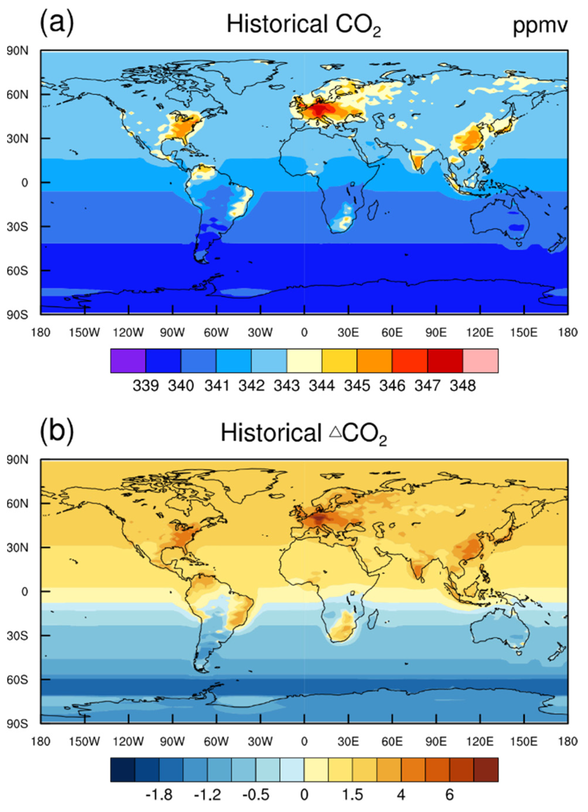
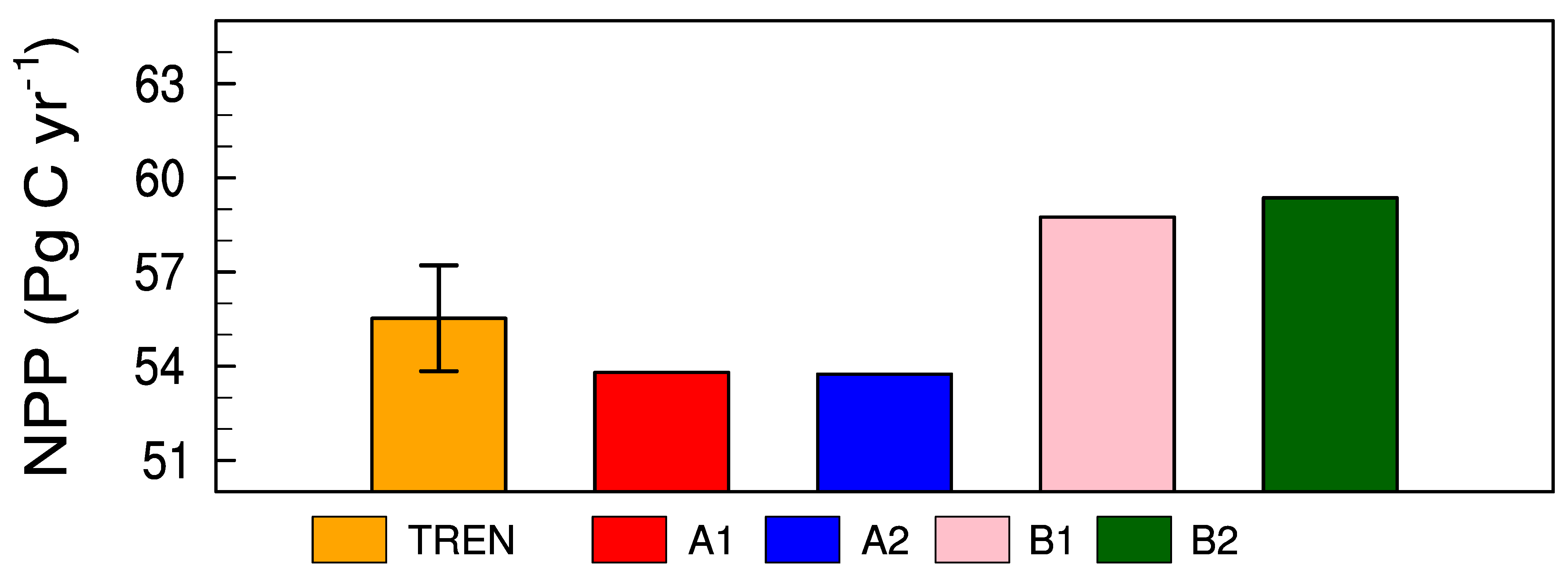
3.1. Estimates of CO₂ Concentrations and NPP

There was a large spatial heterogeneity in atmospheric concentrations of CO₂ between the northern and southern hemispheres in the time period 1956–2005. The non-uniform spatial distribution of CO₂ was lower in Australia, most of Africa and southern South America, but higher in southern Europe, the eastern USA and southeast Asia. During the same time period, simulations A1 and B1 were driven by the same CO₂-radiative forcing and simulations A2 and B2 were enforced by the same CO₂ data. The spatial variations in CO₂ ranged between 339 and 351 ppmv (Figure 2a). Greater differences between simulations A1 and A2 or B1 and B2 were mainly located in southern Europe, the eastern USA and southeast Asia (Figure 2b).

The NPP was estimated for simulations A1, A2, B1 and B2 during the time period 2000–2005 under current conditions. This period was chosen so that our results were comparable with NPP data from the TRENDY datasets. The TRENDY dataset consists of an ensemble of seven process-based terrestrial ecosystem model simulations [36]. We selected experiment S2 without land use changes and fires and including CLM4C, CLM4CN, LPJ, LPJ-GUESS, OCN, SDGVM and TRIFFID [37] from 1901 to 2010.

Our estimated land NPP for the four simulations of 51.39–56.47 Pg C yr⁻¹ was lower than the estimates of about 70 Pg C yr⁻¹ of [38], but higher than the 41 Pg C yr⁻¹ estimated by [39]. The estimated NPPs of the four simulations were closer to the observed estimate of about 56.02 Pg C yr⁻¹ of [40]. Globally, the mean annual NPP in the historical period from CMIP5 was about 62.6 Pg C yr⁻¹ [41], whereas it was 55.53 ± 1.69 Pg C yr⁻¹ from the TRENDY dataset. The mean annual NPP in the historical period simulated by FGOALS-AVIM was 53.80 ± 2.54, 53.75 ± 2.95, 58.75 ± 1.46 and 59.36 ± 2.73 Pg C yr⁻¹ from simulations A1, A2, B1 and B2, respectively (Figure 3).

3.2. Estimates of Climatic Variables under Present Conditions

Over the simulation period 1956–2005, the non-uniform spatial distribution of CO₂ through CO₂-radiative forcing resulted in a global increase in low cloudiness of about 0.002% ± 0.005% (Figure 4a), a net solar flux of 0.52 ± 0.55 W m⁻² including the atmosphere–land–ocean–sea ice dynamics (Figure 4e) and a terrestrial latent heat flux of 0.36 ± 0.97 W m⁻² at the global scale (Figure 4c). At the global scale, the climate variables varied considerably among the different components in response to the non-uniform spatial distribution of CO₂ through CO₂-radiative forcing. During the time period 1956–2005, the non-uniform spatial distribution of CO₂ through CO₂-radiative forcing based on only atmosphere and land interactions caused an increase in the net solar flux of about 0.45 ± 0.31 W m⁻² and a decrease in global low cloudiness of 0.001% ± 0.003%, especially over the ocean (Figure 4b;

Table 3. Response of variables to CO₂-radiative forcing as a result of the non-uniform spatial distribution of CO₂.

Variable	Range	A1–A2	B1–B2
CO2	Global	−0.0007 ± 0.0037
Precipitation (mm yr−1)	Land	6.77 ± 21.45	−9.26 ± 14.72
	Ocean	5.89 ± 14.15	−9.58 ± 9.92
Surface temperature (°C)	Land	0.57 ± 0.45	0.02 ± 0.05
	Ocean	0.45 ± 0.38	0.07 ± 0.08
Latent heat flux (W m−2)	Land	0.59 ± 1.23	−0.64 ± 0.93
	Ocean	0.38 ± 0.80
Sensible heat flux (W m−2)	Land	−0.29 ± 0.46
	Ocean	−0.20 ± 0.42
Net radiation flux at Earth’s surface (W m−2)	Land	0.79 ± 0.69
	Ocean	0.59 ± 0.63
Soil evaporation (kg m−2 yr−1)	Land	3.99 ± 7.52
Vegetation evaporation (kg m−2 yr−1)	Land	0.43 ± 4.90
Soil transpiration (kg m−2 yr−1)	Land	1.91 ± 5.70
Surface runoff	Land	3.00 ± 6.18
Soil moisture (kg m−2)	Land	0.03 ± 0.04

). By contrast, the simulated global latent heat flux based on atmosphere and land interactions decreased by about −0.64 ± 0.93 W m⁻² (Figure 4d).

To further analyze the causes of the differences in the estimated NPP resulting from the non-uniform spatial distribution of CO₂ through CO₂-radiatvie forcing, we estimated the changes in the vital variables (e.g., surface temperature, precipitation, evapotranspiration and soil moisture in the different components) for the historical time period 1956–2005. Non-uniform CO₂ from simulations fully coupled atmosphere–land–ocean–sea ice components caused an increase in surface temperature ranging from 0.57 ± 0.45 °C in the terrestrial ecosystem, where it from simulations only coupled atmosphere and land without active ocean and sea ice components led to less increased surface temperature of 0.02 ± 0.05 °C. The changes in the surface temperature at the regional level correspond well to the changes in the non-uniform spatial distribution of CO₂ considering only the atmosphere–land interactions (Figure 5b). The responses of the surface temperature in tropical regions to the non-uniform spatial distribution of CO₂ through CO₂-radiative forcing based on the fully coupled atmosphere–land–ocean–sea ice components were up to >0.2 °C, especially in the Amazon basin, central Africa and tropical Asia. By contrast, the simulations with only the atmosphere–land interactions simulated a small increase or even decrease in these regions.

In the time period 1956–2005, precipitation over the land surface increased in most of the northern hemisphere, but not in southern Europe, the eastern USA and southeast Asia. This was a response to the non-uniform spatial distribution of CO₂ through CO₂-radiative forcing (Figure 5c) compared with the uniform spatial distribution of CO₂ in the same period. The simulated increase in precipitation influenced by non-uniform spatial distribution of CO₂ considering the full atmosphere–land–ocean–sea ice interactions was much greater than that which considered only atmosphere–land interactions, apart from in the Amazon basin and tropical Asia. This was a result of the larger increase in the net radiation flux from surface warming and latent heat flux over land, especially in the northern hemisphere.

Correspondingly, the responses of the simulated change in evapotranspiration by the two differently coupled components differed considerably in both the direction and magnitude of change for most terrestrial ecosystems (Figure 5d,e). The two different components predicted an increase in evapotranspiration affected by the non-uniform spatial distribution of CO₂ through CO₂-radiative forcing relative to the uniform spatial distribution of CO₂ for most land surfaces. The simulated response of evapotranspiration to changes in the non-uniform spatial distribution of CO₂ differed at the regional scale. For example, evapotranspiration north of 50° N in the northern hemisphere was predicted to increase as a response to the uniform spatial distribution of CO₂ through CO₂-radiative forcing based on the fully coupled atmosphere–land–ocean–sea ice model, but to decrease in southern Europe, the eastern USA and southeast Asia. By contrast, evapotranspiration influenced by the non-uniform spatial distribution of CO₂ considering only the atmosphere–land interactions showed a much greater increase than the fully coupled atmosphere–land–ocean–sea ice interactions at low latitudes and in the eastern USA.

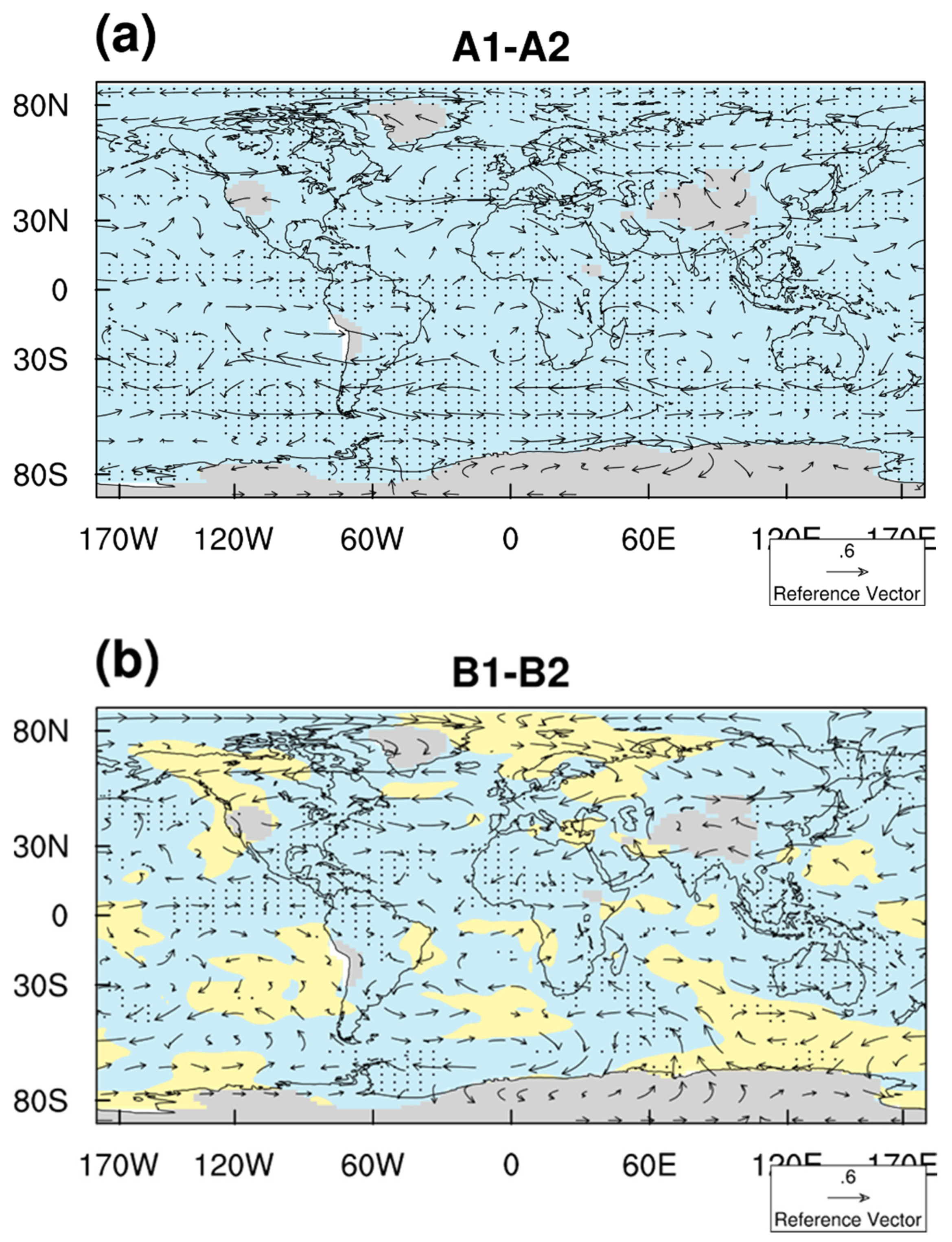
3.3. Responses of NPP to Spatial Varying of CO₂ Concentrations through Radiative Forcing

To quantify the impact of the non-uniform spatial distribution of CO₂ on NPP, we simulated the NPP for the time period 1956–2005 with or without the uniform spatial distribution of CO₂ after 1850. Specifically, we ran FGOALS-AVIM with CO₂ held at the same value at the global level for each land grid point in simulation A2 or B2 and compared the results with the non-uniform spatial distribution of CO₂ for each land grid point in simulation A1 or B1 for the time period 1956–2005.

We estimated that the decrease in NPP caused by the non-uniform spatial distribution of CO₂ through CO₂-radiative forcing during the time period 1956–2005 was −3.39 ± 12.33 g C m⁻² yr⁻¹ or about −0.5 ± 1.88 Pg C yr⁻¹ for the fully coupled atmosphere–land–ocean–sea ice components (simulation A1 minus A2). The increase was about 0.88 ± 8.86 g C m⁻² yr⁻¹ or 0.1 ± 1.35 Pg C yr⁻¹ when considering only atmosphere–land interactions (Figure 6a,b).

The fully coupled atmosphere–land–ocean–sea ice components estimated a decrease in NPP caused by the non-uniform spatial distribution of CO₂ through CO₂-radiative forcing for terrestrial ecosystems (Figure 6a), whereas the coupled active atmosphere–land components predicted an increase (Figure 6b). The mechanism contributing to the estimated change in NPP was similar between the two simulations. With the simulated decrease in soil moisture (Figure 6c), the model based on the fully coupled atmosphere–land–ocean–sea ice components estimated a decrease in NPP for southern Europe, the eastern USA, southeast Asia, the Amazon basin and central Africa (Figure 6a). However, the simulation considering only the atmosphere–land interaction estimated an increase in soil moisture (Figure 4d) for the eastern USA, the Amazon basin and central Africa (Figure 6d). The estimated increase in NPP for these regions using only the active atmosphere–land components was attributed to the relatively higher increase in NPP (Figure 6b).

We used the present vegetation cover for the period of the 1990s based on the plant functional types (PFTs) of the International Geosphere Biosphere Program (IGBP) data [42]. At the PFT-level, the NPP simulated by simulations A due to spatial varying in CO₂ concentrations were reduced for EBF, DBF, C4 and crop, but increased for tundra. The variations in NPP simulated from simulations A and B were feeble for ENF. Globally, the changes of annual NPP from 1956 to 2005 resulting from varying in CO₂ concentrations was ~−0.5 Pg C yr⁻¹ from simulations A or estimates of ~0.1 Pg C yr⁻¹ from simulations B (Supplementary Materials Figure S1).

The non-uniformity of CO₂ leads to substantial changes in surface temperature and water fluxes, and the changes caused by non-uniformity of CO₂ in NPP depend on changes in surface temperature and soil moisture, rather than the impact of CO₂, which may lead to changes in the spatial distribution of NPP (Figure 7). Figure 7b,e show how much change in NPP is locally related to changes in surface temperature, especially in the tropics and the Southern Hemisphere. Obviously, these two variables are significantly correlated, which indicates that changes in surface temperature can explain the changes in NPP in these regions. For example, considering that the fully coupled land-atmosphere-ocean-ice interaction, rising surface temperature leads to negative changes of NPP in tropics due to non-uniform CO₂. On the contrary, in most terrestrial ecosystems, there is a significantly positive correlation between soil moisture and local NPP (p < 0.05) (Figure 7c,f). Therefore, our results indicate that the competition between the impacts of surface temperature and soil moisture on NPP is one of the mechanisms leading to changes in NPP in the tropics.

Although the absolute change in CO₂ at the global scale was estimated to be only about 0.3%, the model based on coupled components A1 minus A2 or B1 minus B2 estimated an additional change in NPP caused by the non-uniform spatial distribution of CO₂ by 14.26% or 11.51% during the time period 1956–2005 (Figure 8). This reflects that the impact of CO₂ heterogeneity on carbon cycle was amplified by the climate effect. In addition, the difference between the two different coupled components probably reflects the contribution of the ocean and sea ice to the climate system. With global warming caused by the non-uniform spatial distribution of CO₂ through CO₂-radiative forcing, the model based on the fully coupled components A1 minus A2 estimated absolute variations in NPP caused by the non-uniform spatial distribution of CO₂ relative to the global NPP driven by a uniform spatial distribution of CO₂ ranging from 0.97 to 1.53% for C3 and from 2.92 to 4.03% for crops. The simulation with only atmosphere–land interactions ranged from 1.76 to 2.23% for C3 and from 2.56 to 3.32% for crops. For different PFTs (e.g., crops), the absolute changes in CO₂ from 0.05 to 0.10% were estimated to be higher than those for other PFTs. The impact of the non-uniform spatial distribution of CO₂ was largest for deciduous broadleaf forest, for which simulation A1 minus A2 estimated higher absolute changes in NPP from 2.53 to 4.65% for evergreen broadleaf forest due to the non-uniform spatial distribution of CO₂, compared with simulation B1 minus B2 from 1.93 to 3.05%. For crops, both simulations A1 minus A2 and B1 minus B2 estimated high absolute changes ranging from 2.56 to 3.32%.

4. Discussion

At present, few studies have considered effect of radiative forcing of spatial varying of CO₂ concentrations in the atmosphere on NPP. Our results showed that the non-uniform spatial distribution of CO₂ through CO₂-radiative forcing has important implications for carbon fluxes. We estimated that the non-uniform spatial distribution of CO₂ contributed to a decrease in NPP, although most other studies have not considered this. The CMIP5 provides an ensemble mean annual NPP of 62.6 Pg C yr⁻¹ over the time period 1995–2004 [41]. However, this analysis did not consider the feedbacks from the non-uniform spatial distribution of CO₂ to the Earth’s climate system. Our analysis showed an effect of the non-uniform spatial distribution of CO₂ on NPP without considering land use of up to 14.26 ± 2.22% of the NPP simulated by a fully coupled model. This highlights the tremendous leverage of a non-uniform spatial distribution of CO₂ on the global carbon cycle and we recommend a more substantial focus on understanding this process in the biosphere through the influence of the climate system based on coupled models that include dynamical sea ice and ocean components.

In the past 30 years, there has been an increase in NPP at the global scale, which is likely driven by CO₂ fertilization [34,35]. However, the increase in CO₂ radiative forcing limits this positive effect [1]. The exact impact of spatial varying in CO₂ concentration on the carbon cycle through radiative forcing is not yet fully understood. Our study illuminates that from 1956 to 2005, the spatial varying in the CO₂ concentration resulted in a reduction of NPP, which mainly occurred in the tropics and the middle-latitudes of the Northern Hemisphere. Nevertheless, as shown in Figure 7, a relationship between variations in CO₂ concentration and NPP could not pass a significant level. It might result due to not considering the impact of CO₂ fertilization. On the contrary, spatial varying in CO₂ concentration through the radiation effect influences temperature, precipitation and soil moisture, which ultimately affects NPP. The northern hemisphere accounts for nearly 68% of the global area, which has a higher CO₂ concentration than the globally averaged level. Higher temperature has a negative impact on NPP in tropics and mid-latitudes of the Northern Hemisphere [33,38,43,44]. In addition, considering ocean feedback, an increase in temperature could reduce NPP in these regions. Conversely, when the ocean feedback is shielded, increases in temperature is slight in tropics. At the same time, in this condition, the increase in the soil moisture would offset the negative impact of warming in tropics.

To estimate the contribution of the ocean and sea ice influenced by the spatial varying of CO₂ concentrations through CO₂-radiative forcing to the terrestrial NPP, we carried out simulations B1 and B2, in which the effect of CO₂-radiative forcing was assessed using fixed the sea surface temperature (SST) in 1980. The additional increase in SST was estimated to be 0.45 ± 0.38 °C using the fully coupled model, compared with 0.07 ± 0.08 °C based on only the coupled active atmosphere–land components. This can be understood by the positive feedback from a greater increase in the SST (Figure 9a) to surface temperature from simulations A1 minus A2 relative to from simulations B1minus B2 without varying SST. The response of NPP in low-latitudes of terrestrial ecosystem to changes in surface temperature might be asymmetric. This may also lead to asymmetric NPP changes related to SST changes. For example, in some tropical terrestrial regions, increased SST has a negative impact on NPP under warmer changes [45]. Therefore, more detailed quantification is needed to understand the asymmetric response of NPP to SST changes.

The spatial response of soil moisture differed widely, although the SST had a key influence soil moisture [46]. Under warmer conditions, a non-uniform spatial distribution of CO₂ decreased soil moisture across the eastern USA, southern Europe and southeast Asia in the fully coupled model. This is consistent with previous research [47], which showed that an increased SST in the tropics would increase the depletion of soil moisture in the eastern USA, southern Europe, southeast Asia and the tropics.

At high latitudes (e.g., the Arctic), the decrease in the area of ice as a result of the non-uniform spatial distribution of CO₂ through CO₂-radiative forcing is >2% (Figure 9b). An additional increase in precipitation has been shown in most of this region. This change can be explained by emergent positive feedbacks between the increasing area of melted ice and the increased water vapor at high latitudes in the fully coupled model. Recent studies have found that a decrease in Arctic sea ice has an important role in the Earth’s climate and ecosystems [48]. Specifically, stronger warming results in an increased loss of sea ice, which, in turn, simulates more melting through a reduced albedo [48]. Ice-loss feedback could amplify changes in the Earth’s climate at high latitudes [48,49]. We estimated larger increases in surface temperature and precipitation for tundra regions using the fully coupled model including sea ice dynamics than the model without sea ice dynamics. There is a positive feedback from an increase in melted sea ice in a warmer and wetter climate, which enhances the NPP by the non-uniform spatial distribution of CO₂ through CO₂-radiative forcing in the tundra regions.

This finding is consistent with a previous study of CO₂-radiative forcing and has important implications for our understanding of the changes in carbon flux associated with climate change [50]. Changes in the non-uniform spatial distribution of CO₂ concentrations influenced changes in the heat budget (Figure 4), then continued to regulate the spatial distribution of surface climate variables. Changes in the atmospheric circulation (Figure 10) introduced by the non-uniform spatial distribution of CO₂ also could influence the water balance and, in turn, affect soil moisture. Therefore, the patterns and responses of the water budget at the regional scales triggered by the non-uniform spatial distribution of CO₂ determine the patterns and responses in NPP. In particular, near-global increases in specific humidity do not mean that this increase necessarily results in an increase in precipitation. The simulation using the fully coupled model estimated that weaker westerlies reduced the input of humid air from the Atlantic Ocean to southern Europe, which reduced precipitation and then increased the depletion of soil moisture. The eastward radial circulation in the eastern USA was strengthened. Such a circulation pattern does not favor precipitation. The eastward radial circulation was also enhanced in East Asia and suppressed the monsoon from the Eastern Pacific Ocean, limiting precipitation and inducing droughts.

CO₂-physiological forcing could also have significant impact on the spatial variation of NPP [51]. However, it was not included in our results, because our main focus is on the impacts of CO₂ radiative forcing on NPP. For terrestrial processes, atmospheric CO₂ was uniformly applied to all PFTs at a fixed level of 355 ppmv. The impact of a spatial variation in CO₂ concentrations was masked in our analysis. Results may be different if we include a variation in the spatiotemporal distribution of atmospheric CO₂ through CO₂-physiological forcing in the land component. This needs further investigation.

5. Conclusions

This study investigated the regulations of spatial varying in atmospheric CO₂ concentration through radiative forcing to annual NPP. The results implied that soil moisture resulting from spatial varying in CO₂ concentration dominates the changes of annual NPP, and the increased SST substantially reduced NPP in tropics. As a consequence, spatial varying of atmospheric CO₂ concentration did change the spatial pattern of NPP under the historical conditions from 1956 to 2005. In addition, our results showed the current offline terrestrial models only considering land and atmosphere interactions did not reproduce the feedback of ocean and sea ice to changes in NPP. In general, this study represented the key role of spatial varying in CO₂ concentration in regulating variations in NPP.

References

1. Friedlingstein, P.; Meinshausen, M.; Arora, V.K.; Jones, C.D.; Anav, A.; Liddicoat, S.K.; Knutti, R. Uncertainties in CMIP5 Climate Projections due to Carbon Cycle Feedbacks. J. Clim. 2013, 27, 511–526. [Google Scholar] [CrossRef] [Green Version]
2. Friedlingstein, P. Carbon cycle feedbacks and future climate change. Philos. Trans. R. Soc. A Math. Phys. Eng. Sci. 2015, 373, 20140421. [Google Scholar] [CrossRef] [PubMed] [Green Version]
3. Govindasamy, B.; Caldeira, K. Geoengineering Earth’s radiation balance to mitigate CO2-induced climate change. Geophys. Res. Lett. 2000, 27, 2141–2144. [Google Scholar] [CrossRef]
4. Etminan, M.; Myhre, G.; Highwood, E.J.; Shine, K.P. Radiative forcing of carbon dioxide, methane, and nitrous oxide: A significant revision of the methane radiative forcing. Geophys. Res. Lett. 2016, 43, 12614–12623. [Google Scholar] [CrossRef]
5. Yuan, W.; Zheng, Y.; Piao, S.; Ciais, P.; Lombardozzi, D.; Wang, Y.; Ryu, Y.; Chen, G.; Dong, W.; Hu, Z.; et al. Increased atmospheric vapor pressure deficit reduces global vegetation growth. Sci. Adv. 2019, 5, eaax1396. [Google Scholar] [CrossRef] [PubMed] [Green Version]
6. Schimel, D.; Stephens, B.B.; Fisher, J.B. Effect of increasing CO2 on the terrestrial carbon cycle. Proc. Natl. Acad. Sci. USA 2015, 112, 436–441. [Google Scholar] [CrossRef] [PubMed] [Green Version]
7. Huang, Y.; Xia, Y.; Tan, X. On the pattern of CO2 radiative forcing and poleward energy transport. J. Geophys. Res. Atmos. 2017, 122, 10578–10593. [Google Scholar] [CrossRef] [Green Version]
8. Myhre, G.; Shindell, D.; Bréon, F.-M.; Collins, W.; Fuglestvedt, J.; Huang, J.; Koch, D.; Lamarque, J.-F.; Lee, D.; Mendoza, B.; et al. Anthropogenic and Natural Radiative Forcing. In Climate Change 2013: The Physical Science Basis. Contribution of Working Group I to the Fifth Assessment Report of the Intergovernmental Panel on Climate Change; Cambridge University Press: Cambridge, UK, 2013. [Google Scholar]
9. Taylor, K.E.; Stouffer, R.J.; Meehl, G.A. An overview of CMIP5 and the Experiment Design. Bull. Am. Meteorol. Soc. 2011, 93, 485–498. [Google Scholar] [CrossRef] [Green Version]
10. Nassar, R.; Napier-Linton, L.; Gurney, K.R.; Andres, R.; Oda, T.; Vogel, F.; Deng, F. Improving the temporal and spatial distribution of CO2 emissions from global fossil fuel emission data sets. J. Geophys. Res. Atmos. 2013, 118, 917–933. [Google Scholar] [CrossRef]
11. Falahatkar, S.; Mousavi, S.M.; Farajzadeh, M. Spatial and temporal distribution of carbon dioxide gas using GOSAT data over IRAN. Environ. Monit. Assess. 2017, 189, 627. [Google Scholar] [CrossRef]
12. Wang, Y.; Feng, J.; Dan, L.; Lin, S.; Tian, J. The impact of uniform and nonuniform CO2 concentrations on global climatic change. Theor. Appl. Climatol. 2019, 139, 45–55. [Google Scholar] [CrossRef]
13. Friedlingstein, P.; Cox, P.; Betts, R.; Bopp, L.; von Bloh, W.; Brovkin, V.; Cadule, P.; Doney, S.; Eby, M.; Fung, I.; et al. Climate–Carbon Cycle Feedback Analysis: Results from the C4MIP Model Intercomparison. J. Clim. 2006, 19, 3337–3353. [Google Scholar] [CrossRef]
14. Ramaswamy, V.; Collins, W.; Haywood, J.; Lean, J.; Mahowald, N.; Myhre, G.; Naik, V.; Shine, K.P.; Soden, B.; Stenchikov, G.; et al. Radiative Forcing of Climate: The Historical Evolution of the Radiative Forcing Concept, the Forcing Agents and their Quantification, and Applications. AMS Meteorol. Monogr. 2019, 59, 14.1–14.101. [Google Scholar] [CrossRef]
15. Ballantyne, A.; Smith, W.; Anderegg, W.; Kauppi, P.; Sarmiento, J.; Tans, P.; Shevliakova, E.; Pan, Y.; Poulter, B.; Anav, A.; et al. Accelerating net terrestrial carbon uptake during the warming hiatus due to reduced respiration. Nat. Clim. Chang. 2017, 7, 148–152. [Google Scholar] [CrossRef]
16. Cox, P.; Pearson, D.; Booth, B.; Friedlingstein, P.; Huntingford, C.; Jones, C.; Luke, C. Sensitivity of tropical carbon to climate change constrained by carbon dioxide variability. Nature 2013, 494, 341–344. [Google Scholar] [CrossRef] [PubMed]
17. Peng, J.; Dan, L.; Dong, W. Are there interactive effects of physiological and radiative forcing produced by increased CO2 concentration on changes of land hydrological cycle? Glob. Planet. Chang. 2014, 112, 64–78. [Google Scholar] [CrossRef] [Green Version]
18. IPCC. Climate Change 2014: Synthesis Report. In Contribution of Working Groups I, II and III to the Fifth Assessment Report of the Intergovernmental Panel on Climate Change; IPCC: Geneva, Switzerland, 2014; p. 151. [Google Scholar]
19. Zhou, T.; Song, F.; Chen, X. Historical evolution of global and regional surface air temperature simulated by FGOALS-s2 and FGOALS-g2: How reliable are the model results? Adv. Atmos. Sci. 2013, 30, 638–657. [Google Scholar] [CrossRef]
20. Dan, L.; Cao, F.; Gao, R. The improvement of a regional climate model by coupling a land surface model with eco-physiological processes: A case study in 1998. Clim. Chang. 2015, 129, 457–470. [Google Scholar] [CrossRef] [Green Version]
21. Ahlström, A.; Raupach, M.R.; Schurgers, G.; Smith, B.; Arneth, A.; Jung, M.; Reichstein, M.; Canadell, J.G.; Friedlingstein, P.; Jain, A.K.; et al. The dominant role of semi-arid ecosystems in the trend and variability of the land CO2 sink. Science 2015, 348, 895–899. [Google Scholar] [CrossRef] [Green Version]
22. Bao, Q.; Lin, P.; Zhou, T.; Liu, Y.; Yu, Y.; Wu, G.; He, B.; He, J.; Li, L.; Li, J.; et al. The Flexible Global Ocean-Atmosphere-Land system model, Spectral Version 2: FGOALS-s2. Adv. Atmos. Sci. 2013, 30, 561–576. [Google Scholar] [CrossRef]
23. Grise, K.M.; Polvani, L.M. Understanding the Time Scales of the Tropospheric Circulation Response to Abrupt CO2 Forcing in the Southern Hemisphere: Seasonality and the Role of the Stratosphere. J. Clim. 2017, 30, 8497–8515. [Google Scholar] [CrossRef]
24. Törnqvist, R.; Jarsjö, J.; Pietroń, J.; Bring, A.; Rogberg, P.; Asokan, S.M.; Destouni, G. Evolution of the hydro-climate system in the Lake Baikal basin. J. Hydrol. 2014, 519, 1953–1962. [Google Scholar] [CrossRef] [Green Version]
25. Ji, J.; Hu, Y. A simple land surface process model for use in climate study. J. Meteorol. Res. 1989, 3, 342–351. [Google Scholar]
26. Ji, J.; Huang, M.; Li, K. Prediction of carbon exchanges between China terrestrial ecosystem and atmosphere in 21st century. Sci. China Ser. D-Earth Sci. 2008, 51, 885–898. [Google Scholar] [CrossRef]
27. Wang, J.; Bao, Q.; Zeng, N.; Liu, Y.; Wu, G.; Ji, D. Earth System Model FGOALS-s2: Coupling a dynamic global vegetation and terrestrial carbon model with the physical climate system model. Adv. Atmos. Sci. 2013, 30, 1549–1559. [Google Scholar] [CrossRef]
28. Peng, J.; Dan, L. The Response of the Terrestrial Carbon Cycle Simulated by FGOALS-AVIM to Rising CO2. In Flexible Global Ocean-Atmosphere-Land System Model; Springer: Berlin/Heidelberg, Germany, 2014; pp. 393–403. [Google Scholar]
29. Oda, T.; Maksyutov, S.; Andres, R.J. The Open-source Data Inventory for Anthropogenic CO2, version 2016 (ODIAC2016): A global monthly fossil fuel CO2 gridded emissions data product for tracer transport simulations and surface flux inversions. Earth Syst. Sci. Data 2018, 10, 87–107. [Google Scholar] [CrossRef] [Green Version]
30. Peng, J.; Wang, Y.; Houlton, B.Z.; Dan, L.; Pak, B.; Tang, X. Global Carbon Sequestration Is Highly Sensitive to Model-Based Formulations of Nitrogen Fixation. Glob. Biogeochem. Cycles 2020, 34, e2019GB006296. [Google Scholar] [CrossRef]
31. Peng, J.; Dan, L. Impacts of CO2 concentration and climate change on the terrestrial carbon flux using six global climate-carbon coupled models. Ecol. Model. 2015, 304, 69–83. [Google Scholar] [CrossRef]
32. Peng, J.; Dan, L.; Yang, F.; Tang, X.; Wang, D. Global and regional estimation of carbon uptake using CMIP6 ESM compared with TRENDY ensembles at the centennial scale. J. Geophys. Res. Atmos. 2012, 126, e2021JD035135. [Google Scholar] [CrossRef]
33. Peng, J.; Peng, J.; Dan, L.; Ying, K.; Yang, S.; Tang, X.; Yang, F. China’s Interannual Variability of Net Primary Production Is Dominated by the Central China Region. J. Geophys. Res. Atmos. 2021, 126, e2020JD033362. [Google Scholar] [CrossRef]
34. Sitch, S.; Friedlingstein, P.; Gruber, N.; Jones, S.D.; Murray-Tortarolo, G.; Ahlström, A.; Doney, S.C.; Graven, H.; Heinze, C.; Huntingford, C.; et al. Recent trends and drivers of regional sources and sinks of carbon dioxide. Biogeosciences 2015, 12, 653–679. [Google Scholar] [CrossRef] [Green Version]
35. Friedlingstein, P.; Friedlingstein, P.; O’sullivan, M.; Jones, M.W.; Andrew, R.M.; Hauck, J.; Olsen, A.; Peters, G.P.; Peters, W.; Pongratz, J.; et al. Global Carbon Budget 2020. Earth Syst. Sci. Data 2020, 12, 3269–3340. [Google Scholar] [CrossRef]
36. Zhang, X.; Rayner, P.; Wang, Y.; Silver, J.D.; Lu, X.; Pak, B.; Zheng, X. Linear and nonlinear effects of dominant drivers on the trends in global and regional land carbon uptake: 1959 to 2013. Geophys. Res. Lett. 2016, 43, 1607–1614. [Google Scholar] [CrossRef] [Green Version]
37. Piao, S.; Sitch, S.; Ciais, P.; Friedlingstein, P.; Peylin, P.; Wang, X.; Ahlström, A.; Anav, A.; Canadell, J.; Cong, N.; et al. Evaluation of terrestrial carbon cycle models for their response to climate variability and to CO2 trends. Glob. Chang. Biol. 2013, 19, 2117–2132. [Google Scholar] [CrossRef] [Green Version]
38. Piao, S.; Ciais, P.; Friedlingstein, P.; de Noblet-Ducoudré, N.; Cadule, P.; Viovy, N.; Wang, T. Spatiotemporal patterns of terrestrial carbon cycle during the 20th century. Glob. Biogeochem. Cycles 2009, 23. [Google Scholar] [CrossRef]
39. Thornton, P.; Zimmermann, N. An Improved Canopy Integration Scheme for a Land Surface Model with Prognostic Canopy Structure. J. Clim. 2007, 20, 3902–3923. [Google Scholar] [CrossRef]
40. Zhao, M.; Heinsch, F.A.; Nemani, R.R.; Running, S.W. Improvements of the MODIS terrestrial gross and net pri-mary pro-duction global data set. Remote Sens. Environ. 2005, 95, 164–176. [Google Scholar] [CrossRef]
41. Wieder, W.; Cleveland, C.C.; Smith, W.; Todd-Brown, K. Future productivity and carbon storage limited by terrestrial nutrient availability. Nat. Geosci. 2015, 8, 441–444. [Google Scholar] [CrossRef]
42. Loveland, T.R.; Reed, B.C.; Brown, J.F.; Ohlen, D.O.; Zhu, Z.; Yang, L.W.M.J.; Merchant, J.W. Development of a global land characteristics database and IGBP DISCover from 1 km AVHRR data. Int. J. Remote Sens. 2000, 21, 1303–1330. [Google Scholar] [CrossRef]
43. Fernández-Martínez, M.; Sardans, J.; Chevallier, F.; Ciais, P.; Obersteiner, M.; Vicca, S.; Canadell, J.G.; Bastos, A.; Friedlingstein, P.; Sitch, S.; et al. Global trends in carbon sinks and their relationships with CO2 and temperature. Nat. Clim. Chang. 2019, 9, 73–79. [Google Scholar] [CrossRef] [Green Version]
44. Piao, S.; Wang, X.; Park, T.; Chen, C.; Lian, X.; He, Y.; Bjerke, J.; Chen, A.; Ciais, P.; Tømmervik, H.; et al. Characteristics, drivers and feedbacks of global greening. Nat. Rev. Earth Environ. 2020, 1, 14–27. [Google Scholar] [CrossRef]
45. Kim, I.-W.; Stuecker, M.F.; Timmermann, A.; Zeller, E.; Kug, J.-S.; Park, S.-W.; Kim, J.-S. Tropical Indo-Pacific SST influences on vegetation variability in eastern Africa. Sci. Rep. 2021, 11, 10462. [Google Scholar] [CrossRef] [PubMed]
46. Mei, R.; Wang, G. Impact of Sea Surface Temperature and Soil Moisture on Summer Precipitation in the United States Based on Observational Data. J. Hydrometeorol. 2011, 12, 1086–1099. [Google Scholar] [CrossRef]
47. Dai, A. Increasing drought under global warming in observations and models. Nat. Clim. Chang. 2013, 3, 52–58. [Google Scholar] [CrossRef]
48. Meier, W.N.; Hovelsrud, G.K.; Van Oort, B.E.; Key, J.R.; Kovacs, K.M.; Michel, C.; Haas, C.; Granskog, M.; Gerland, S.; Perovich, D.K.; et al. Arctic sea ice in transformation: A review of recent observed changes and impacts on biology and human activity. Rev. Geophys. 2014, 52, 185–217. [Google Scholar] [CrossRef]
49. Dai, A.; Luo, D.; Song, M.; Liu, J. Arctic amplification is caused by sea-ice loss under increasing CO2. Nat. Commun. 2019, 10, 121. [Google Scholar] [CrossRef] [Green Version]
50. Cao, L.; Bala, G.; Caldeira, K.; Nemani, R.; Ban-Weiss, G. Importance of carbon dioxide physiological forcing to future cli-mate change. Proc. Natl. Acad. Sci. USA 2010, 107, 9513–9518. [Google Scholar] [CrossRef] [Green Version]
51. Swann, A.L.S.; Hoffman, F.M.; Koven, C.D.; Randerson, J.T. Plant responses to increasing CO2 reduce estimates of climate impacts on drought severity. Proc. Natl. Acad. Sci. USA 2016, 113, 10019–10024. [Google Scholar] [CrossRef] [Green Version]
Figure 1. Geographical distribution of the 10 plant function types in FGOALS-AVIM. ENF, evergreen needle leaf forest; EBF, evergreen broadleaf forest; DBF, deciduous broadleaf forest.
Sustainability 13 10897 g001
Figure 2. (a) Spatial variation in the mean annual atmospheric CO2 concentrations during the time period 1956-2005 estimated by FGOALS-AVIM. (b) Mean annual changes in CO2 concentrations during the time period 1956–2005 estimated by simulation A1 relative to A2 or simulation B1 relative to B2.
Sustainability 13 10897 g002
Figure 3. From 1956 to 2005, comparison of different estimates of net primary production based on the TRENDY ensemble (TREN, orange bar) taking into consideration the spatial heterogeneity of atmospheric CO2 concentrations in the fully coupled atmosphere–land–ocean–sea ice components of FGOALS-AVIM (A1, red bar), the fully coupled atmosphere–land–ocean–sea ice components of FGOALS-AVIM without the spatial heterogeneity of atmospheric CO2 concentrations (A2, blue bar), the spatial heterogeneity of atmospheric CO2 concentrations with only atmosphere–land coupling in FGOALS-AVIM (B1, prink bar) and only atmosphere–land coupling without the spatial heterogeneity of atmospheric CO2 concentrations (B2, green bar).
Sustainability 13 10897 g003
Figure 4. (a,b) Response of the mean annual low cloudiness to the spatial heterogeneity of CO2 concentrations over the time period 1956–2005 estimated from simulation A1 or B1 relative to A2 or B2, respectively. (c,d) Spatial changes in the mean annual net solar flux at the Earth’s surface estimated from simulation A1 or B1 relative to A2 or B2, respectively. (e,f) Spatial changes in the mean annual latent heat flux estimated from simulation A1 or B1 relative to A2 or B2, respectively.
Sustainability 13 10897 g004
Figure 5. (a,b) Response of the mean annual surface temperature to the spatial heterogeneity of CO2 concentrations over the time period 1956–2005 estimated from simulation A1 or B1 relative to A2 or B2, respectively. (c,d) Spatial changes in precipitation estimated from simulation A1 or B1 relative to A2 or B2, respectively. (e,f) Spatial changes in the mean evapotranspiration estimated from simulation A1 or B1 relative to A2 or B2, respectively.
Sustainability 13 10897 g005
Figure 6. (a,b) Response of the mean net primary production to the spatial heterogeneity of CO2 concentrations over the time period 1956–2005 estimated from simulation A1 or B1 relative to A2 or B2, respectively. (c,d) Spatial changes in soil moisture estimated from simulation A1 minus A2 or B1 minus B2, respectively.
Sustainability 13 10897 g006
Figure 7. (ac) Linear correlation coefficients of changes in CO2 concentrations, the surface temperature (TS), soil moisture (MRSO) to NPP over the time period 1956–2005 estimated from simulation A1 relative to A2, respectively. (df) Linear correlation coefficients of changes in CO2 concentrations, the surface temperature (TS), soil moisture (MRSO) to NPP over the time period 1956–2005 estimated from simulation B1 relative to B2, respectively. Dotted areas are areas with statistically significant changes at the 5% level using Student’s t-test.
Sustainability 13 10897 g007
Figure 8. Changes in (a) CO2 concentrations (units: %) and (b) net primary production (NPP) (units: %) over the time period 1956–2005 from simulation A1 or B1 relative to A2 or B2 as estimated using FGOALS-AVIM over different plant function types. ENF, evergreen needle leaf forest; EBF, evergreen broadleaf forest; DBF, deciduous broadleaf forest; C, C4; Cr, crop; Gl, global. Error bar are ±SD calculated from model simulations over the same time period.
Sustainability 13 10897 g008
Figure 9. Modeled patterns for zonal changes in (a) ocean temperature with depth (units: °C) and (b) the fraction of ice area (units: %) in the time period 1956–2005 in FGOALS-AVIM simulation A1 relative to A2.
Sustainability 13 10897 g009
Figure 10. (a,b) Spatial changes in the mean specific humidity (units: g kg−1) and 850 hPa winds (vectors; m s−1) over the time period 1956–2005 estimated using FGOALS-AVIM from simulation A1 or B1 relative to A2 or B2, respectively. Dotted areas are areas with statistically significant changes at the 5% level using Student’s t-test.
Sustainability 13 10897 g010