
Different Geothermal Power Cycle Configurations Cost Estimation Models


Department of Industrial Engineering, University of Florence, 50134 Firenze, Italy
*
Author to whom correspondence should be addressed.
Sustainability 2021, 13(20), 11133; https://0-doi-org.brum.beds.ac.uk/10.3390/su132011133
Submission received: 21 August 2021
/
Revised: 4 October 2021
/
Accepted: 7 October 2021
/
Published: 9 October 2021
(This article belongs to the Special Issue Sustainable Geothermal Energy)
Abstract
:An economic assessment of different geothermal power cycle configurations to generate cost models is conducted in this study. The thermodynamic and exergoeconomic modeling of the cycles is performed in MATLAB coupled to Refprop. The models were derived based on robust multivariable regression to minimize the residuals by using the genetic algorithm. The cross-validation approach is applied to determine a dataset to examine the model in the training phase for validation and reduce the overfitting problem. The generated cost models are the total cost rate, the plant’s total cost, and power generation cost. The cost models and the relevant coefficients are generated based on the most compatibilities and lower error. The results showed that one of the most influential factors on the ORC cycle is the working fluid type, which significantly affects the final economic results. Other parameters that considerably impact economic models results, of all configurations, are geothermal fluid pressure and temperature and inlet pressure of turbine. Rising the geothermal fluid mass flow rate has a remarkable impact on cost models as the capacity and size of equipment increases. The generated cost models in this study can estimate the mentioned cost parameters with an acceptable deviation and provide a fast way to predict the total cost of the power plants.
1. Introduction
Probably one of the most vital parts of designing a power plant is determining the execution of the project. The cost estimation of a project defines whether the stakeholders and industries progress with the project. Power plant cost estimating is one of the most critical steps in project management. A cost assessment builds the baseline of the project cost at diverse stages of the project’s development. A cost estimation at a particular step of project development expresses a prediction based on available data. In the cost estimation process, there may generally be some uncertainties that can affect the decision of industries. However, the accuracy of cost model estimation can improve using more reliable data and optimization methods. Every power plant project needs a more accurate cost estimation to help investors decide about the investment amount. Every project manager is dependent on realistic cost assessments to allow for successful cost management. Budgeting and cost control is very critical but also challenging under uncertainty. Uncertainty means we do not have all the information about the future, and the suspicions we make today may come out differently as the project progresses [1].
There are downsides to imprecise approximations as they could be overestimated or underestimated; they have adverse effects either way. By correct guesstimates, investors can make sure that the allocated resources can support a specific project. The up-front estimation of the investment costs of a new plant is a challenging task, iterating as the design evolves to increased detail. Underestimation of capital costs occurs mainly due to incomplete listing of all the equipment needed in the process [2]. Applying the whole procedure of exergoeconomic assessment of power plants could be time-consuming and complex, especially for some researchers who want to reach the final results as soon as possible. Then, introducing a fast cost model to predict the economic parameters of the cycle could be helpful. The costs of the major equipment items are generally estimated from publicly available equipment cost correlations, which have been established for many commonly used industrial equipment. For ORC systems, the major equipment items are the main components: the evaporator, expander and generator, condenser, and pump. Because there is little information about the component costs of existing ORC systems, most researchers use publicly available correlations for standard equipment items. The application of geothermal energy and its potential in power generation has been considered by some researchers [3,4,5]. One of the most valuable tools for researchers is the exergy concept that could be implemented to assess geothermal power cycles more precisely to find the critical exergy destruction points [6,7]. This practical tool leads to an increase in the exergetic efficiency of geothermal power plants. El Haj Assad et al. [8] performed an energy and exergy assessment and numerical study of different geothermal power cycles. Dincer and Rosen [9] conducted energy and exergy analysis performance for different renewable energies such as geothermal, solar, and so on.
Some researchers have carried out several studies in order to generate cost models for different equipment or projects. Williams [10] estimated heat exchanger costs by comparing equipment pieces of the same model. Hamilton et al. [11] presented a practice of cost estimation comprised of information and quality. For cost evaluation, they divided the project into three steps: concept, development, and execution. Max et al. [12] conducted equipment sizing and cost estimations for process equipment based on computer-aided design and optimization. They analyzed ten different methods in cost evaluation. Yang [13] proposed a generic method to combine correlations between cost factors within the cost estimating process. The presented method checks correlation feasibility first to see if it requires any adjustment or not. Turton et al. [2] introduced cost correlations of several chemical process devices based on different equipment types, materials, and pressure ranges. Caputo and Pelagagge [14] compared parametric function and artificial neural networks to calculate the cost of large and complex-shaped pressure vessels.
Blankenship and Mansure [15] employed the Sandia National Laboratory database to normalize costs for geothermal wells, based on data for thirty-three wells, and generated the cost correlation of geothermal wells as an exponential function of depth. Ogayar and Vidal [16] developed a series of correlations to estimate the cost of a small hydro-power plant’s electro-mechanical equipment using basic parameters such as power and head. Feng and Rangaiah [17] compared five capital cost estimation programs for several types of equipment. They investigated seven case studies relevant to the petroleum refining, petrochemical, and biopharmaceutical processes. Brotherson et al. [18] tried to identify the best practice in capital cost assessment through interviews with leading corporations and financial advisors. Additionally, their study outlined the varieties of practice with the capital pricing model application, the discussions in favor of diverse approaches, and the practical indications of differing choices. Gunduz and Sahin [19] developed two cost estimation models to evaluate hydroelectric power plant project costs by implementing neural networks and multiple regression assessments in the early project planes. Symister [20] performed capital cost estimations for chemical processing using Aspen capital cost estimator for different equipment types in his thesis.
Caputo et al. [21] expanded an analytical-generative cost estimation procedure by promoting a mathematical model for shell and tube heat exchangers. Torp and Klakegg [1] identified some practical challenges with cost estimation under uncertainty for the decommissioning of the Barsebäck nuclear power plant. They demonstrated some practical solutions for cost estimation and uncertainty investigation in complex projects. Luyben [22] presented a simple method to estimate compressor costs using Aspen. However, he did not implement an optimization method. Gul and Aslanoglu [23] made a numerical study of wells’ drilling and testing cost to predict the drilling cost. They applied the drilling data of twenty wells to estimate the drilling cost trend. Amorim Jr et al. [24] reviewed the previous statistical methodology to estimate the cost of prospective wells. They used a database from an onshore field in Brazil to show the advantages of their approach to developing new drillings. Malhan and Mittal [25] applied a polynomial regression model base to generate cost correlations for the main components in micro hydropower plants. Shamoushaki et al. [26] generated cost models of equipment purchasing for several geothermal power plant components such as pumps, compressors, heat exchangers, air coolers, and pressure vessels. Their proposed cost models were derived based on robust multivariable regression to minimize the residuals using the genetic algorithm. Shamoushaki et al. [27] proposed cost and time models for geothermal well drilling in different world regions. The presented drilling cost models were generated based on the well depth and the number of wells. They also compared various drilling cost portions such as equipment, material, construction, design and project management, insurance and certification, and contingency expenses of different world regions.
The cost models for estimating the total cost rate, plant’s total cost, and power generation cost for different geothermal configurations are generated in this study. The thermodynamic and exergoeconomic modeling of all systems is performed in a MATLAB environment, coupled to Refprop 9.1 (NIST, Gaithersburg, MD, USA) [28]. The most updated equipment costs are applied to generate these models, which are related to the 2020 database that has been presented by Shamoushaki et al. [26]. Other applied cost correlations are updated based on the CEPCI index to consider the inflation rate [29]. The cost data are collected and calculated based on changing the main operational parameters of the cycle and considering their impact on the economic results. The optimization method is applied to reduce the uncertainty and deviations of coefficients and statistical measurements. The generated cost models in this study are able to estimate the mentioned cost parameters with an acceptable deviation and provide a fast way to predict them. This kind of study has not been evaluated before and could be a helpful tool for other researchers and industries to have a fast approximation.
2. Modeling Process
2.1. Energy and Exergy Modeling
The system modeling of the cycles is performed based on the first and second laws of thermodynamic. The mathematical modeling is expanded in MATLAB using Refprop 9.1 [28]. The considered system is modeled under steady-state conditions. Mass and energy balance equations applied for all configurations’ evaluation are as follows:
In the above equations, in and out refer to inlet and outlet, respectively. , , and are mass flow rate kg/s, specific enthalpy kJ/kg, heat transfer, and work, respectively kW. In this study, the kinetic, chemical and potential are presumed ignorable, and just physical exergy are considered in analyzing these systems. The exergy balance equations are written as below [30]:
Here, is the specific exergy of each stream kJ/kg. , and are the exergy of heat transfer, work, and exergy destruction of each component kW, respectively. The same procedure has been performed for all considered configurations. The comprehensive considerations, configurations and equations of the geothermal cycles have been presented by DiPippo [31].
2.2. Exergoeconomic Modeling
Exergoeconomic is a powerful tool that has been created by combining the exergy and economic concepts. The Specific Exergy Costing (SPECO) approach is applied for the exergoeconomic assessment of the cycles [32]. For exergoeconomic modeling of this system, cost balance and auxiliary equations are applied in all evaluated cycles. The equation of cost balance for whole equipment is as [30]:
In this equation, is unit cost rate of heat transfer $/s, is unit cost rate of work $/s and is capital cost rate. and are the inlet and outlet cost units $/s, respectively. The total cost rate of the cycle is the sum of capital investments (CI) and operating and maintenance (O&M) cost, then [30]:
In this equation, , and are investment cost of the kth component ($), maintenance factor, and annual plant working hours (which is considered 7446 h [33]), respectively. is capital recovery factor that its formula has been presented in ref [30]. The purchasing cost correlations and their constant values are brought in Table 1. Here, is the interest rate, which is considered 10% [34], and n is the power plant’s lifetime that is supposed to be 30 years. In the exergoeconomic evaluation, by introducing each component product and fuel, the product and fuel cost of components can be calculated. Moreover, the cost rate related to exergy destruction can be obtained by multiplying specific fuel cost and exergy destruction of each piece of equipment [30].
Here, and are the specific cost of product and fuel $/kJ, respectively. is exergy destruction cost rate of the kth component $/s.
The purchasing cost estimation has a direct impact on the cost models and prediction. Implementing the most accurate and updated equations can reduce errors. The thermodynamic and exergoeconomic analyses of different power plant configurations are carried out by many researchers [34,35,36,37,38,39,40]. After completing the system modeling from energy, exergy, and exergoeconomic points of view, the following economic parameters are calculated [41]:
In the above equations, is total plant cost which is the sum of direct and indirect costs of the power plant such as equipment cost, insurance, O&M, etc., and is total capital investment ($). The applied purchasing equipment cost equations are presented in Table 1. In this table, the unit for power is kW, for the area is m2, for mass flow rate is kg/s and for the intensity of the water flow () is m3/s.
2.3. Methodology
The cost estimation process has common characteristics. The most common features are levels of outline, demands, and methods used. Cost estimation can be applied to any project. It may include consideration of project type (power plant construction, building, etc.), definition level (amount of information available), estimation methods (parametric, definitive). The cost evaluation range (lower and upper ranges) could be defined by assessing each cost factor’s lower and upper spine independently. In the primary steps of establishing and assessing a project, attempts should be directed towards building a better design basis than concentrating on utilizing more detailed estimating methods. A parametric model could be a helpful instrument for developing preliminary conceptual estimates when there is little scientific data to implement a basis for using more precise estimating purposes. A parametric estimation involves cost estimating relations and other cost estimating functions that provide logical and repeatable relationships between independent variables. Capacity and equipment factors are simple examples of parametric estimates; however, sophisticated parametric models typically involve several independent variables. Parametric estimating relies on collecting and analyzing previous project cost data to develop the cost estimating relationships.
In this study, different geothermal configurations are evaluated to generate the economic models based on the net power, area of heat exchangers, and intensity of the water flow of the cooling tower as dependent variables. The considered configurations are simple ORC, single flash, double flash, regenerative ORC, and flash-binary cycles. The schematic diagram of evaluated power cycles can be found in [31]. To obtain the cost data to generate the models, the thermodynamic and exergoeconomic modeling of the power cycles are performed. The cost models presented for binary cycles are generated based on the net power and area. For the flash cycles, three different options are presented for cost models prediction based on different dependent variables. One option is based on the area and net power, the second is based on the area and water flow of the cooling tower, and the third, net work and water flow. The sensitivity assessment showed that these parameters have more significant direct impacts on economic parameters.
Step 1—Primary design: The different geothermal configurations have been designed and selected at the first step. For ORC cycles, different working fluids are chosen to apply in system modeling. The main input parameters to apply in system modeling are selected based on the cycle’s specifications. The input parameters applied in thermodynamic modeling for all cycles are presented in Table 2. The value of these parameters has been presented in Appendix A section (Table A1). Three different economic parameters are considered to estimate according to these variables. These parameters are the total cost rate, the plant’s total cost, and the power generation cost. The total cost rate includes the cost rate related to capital and exergy destruction costs.
Step 2—Thermodynamic modeling: The second step is thermodynamic modeling of all configurations. In this part, the thermodynamic properties of all streams (pressure, temperature, enthalpy, entropy, and mass flow rate) are calculated. By completing the energy and exergy modeling and applying mass and energy balance equations, all equipments’ heat and power capacity and the net power of cycles are calculated. The heat exchangers’ area is calculated using thermodynamic values of each point, and log mean temperature difference (LMTD) definition. For ORC cycles, the modeling is performed according to different main operational parameters such as geothermal temperature and pressure, turbine inlet pressure, condensation temperature, and equipment efficiencies. Additionally, the assessment is performed for different ORC working fluids as the impact of each working fluid on the exergetic and economic performance of the power plants is different. However, for flash cycles, the only working fluid is water. Additionally, based on exergy definition and exergy balance equations for each component, the exergy of each stream, exergy destruction, and efficiency of each component have been calculated.
Step 3—Exergoeconomic modeling: The results obtained from the previous step are applied for exergoeconomic modeling. The most updated purchasing cost model presented by Shamoushaki et al. is applied to calculate the equipment cost. These cost models are generated based on the equipment cost related to the 2020 database. In addition, to estimate the purchasing cost of some of the equipment such as the turbine, expansion valve, and cooling tower, other cost correlations are applied. For these components, the CEPCI factor is applied to consider the inflation rate. The cost of each stream has been calculated using cost balance and auxiliary equations. In addition, exergies and costs of fuel and product have been defined for each piece of equipment. At the end of this step, the economic parameters (three considered parameters) have been obtained, which are implemented for cost model generations. These parameters significantly depend on the design variables and suppose which apply in cycle modeling. Some limitations are defined for operational parameters in modeling and running the cycles’ programming to avoid deviated results.
Step 4—Data collection and lookup table generation: After running code for different operational conditions, the obtained cost data from exergoeconomic assessment are collected as a lookup table to generate the cost models (statistical data in Table 3). By changing the input parameters of each cycle and other relevant parameters, the program has been run iteratively, and output economic results have been put in these lookup tables. The lookup table is produced for each configuration separately. However, to reduce the deviation and data scattering issues, some approaches are applied as the next step.
Step 5—Optimization and model generation: The cross-validation approach is used to examine the collected dataset to decrease the errors. Then, applying the curve fitting process, the most compatible and fitted lines are generated base on the available data. However, a genetic algorithm is implemented to optimize the generated cost correlations and models to minimize the residuals. Finally, the cost models are generated based on the dependent variables. These parameters depend on the input variables values adopted for the simulation of the cycles.
2.4. Optimization
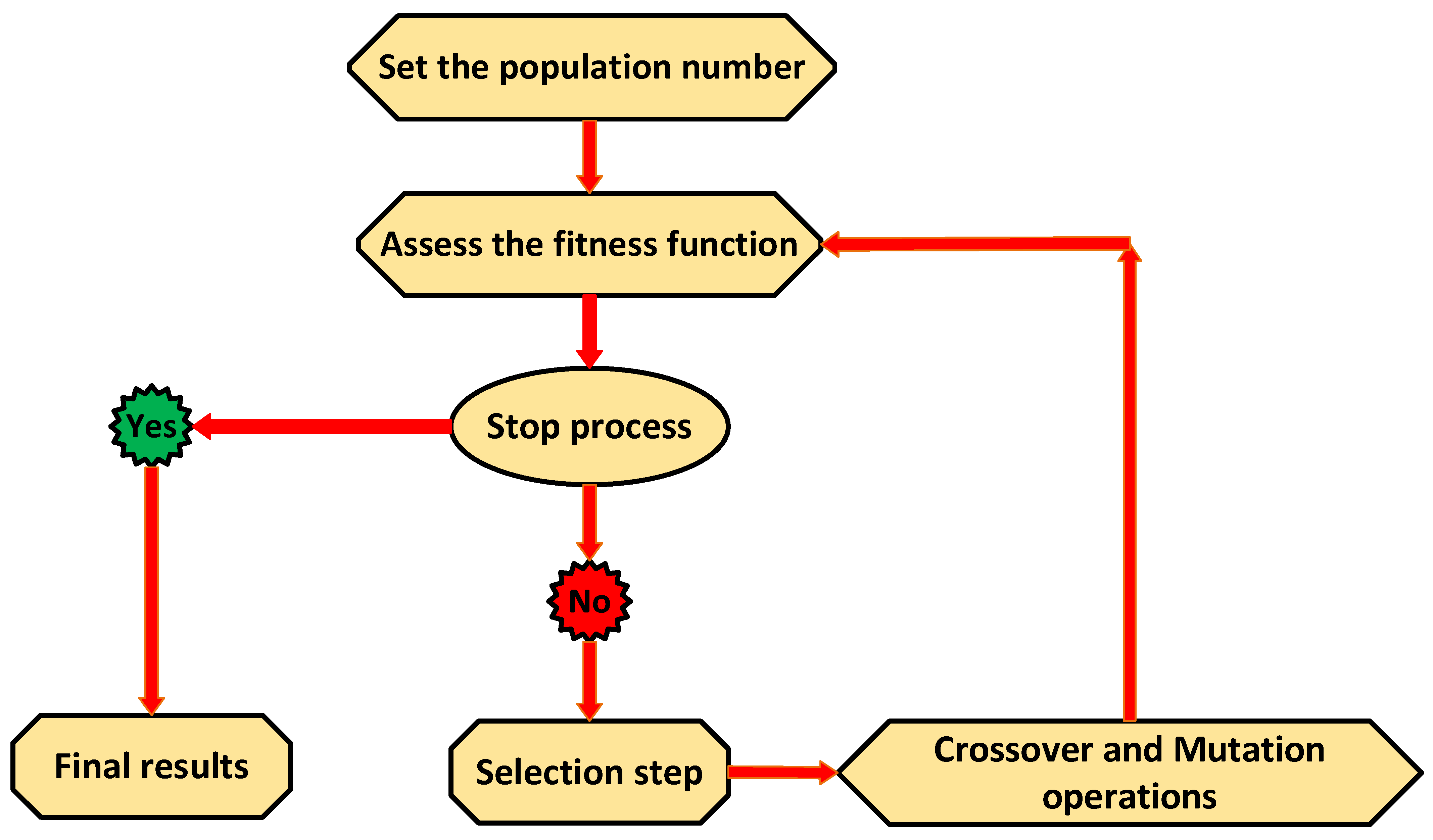
The optimization problems are obtaining responses or responses on a set of possible possibilities to optimize the criterion or criteria of the problem [46]. Genetic algorithms are randomized search algorithms promoted to imitate the mechanics of natural determination and natural genetics [47]. A genetic algorithm is applied to minimizing the independent errors [48]. The considered objective function is as follows [26,48]:
Here, and are calculated as calculated and reference values, respectively. There is no restriction of correlation form and coefficient number in this minimization method [26,48]. The optimization process convergence is obtained within the 5000 iteration limitation. There is no restriction of correlation form and coefficient number in this minimization method [48]. The selected population is different for each configuration, and the generation was considered 300. The mutation and crossover fraction factors were considered to be 0.2 and 0.8, respectively. The genetic algorithm was chosen because of its particular advantages: agreeable convergence rate, suitability for a wide diversity of optimization problems, wide solution space searchability, and facility in determining global optimums and avoiding trapping in local optimal [26]. The flowchart of the genetic algorithm is shown in Figure 1.
2.5. Cross-Validation Approach
When data has been feeding into a machine learning algorithm, the algorithm utilizes the data to distinguish patterns and discover how to reach a more reliable solution. Many algorithms have performance metrics that can be applied to evaluate how robust the model’s learning of the data. Nevertheless, one of the best methods for assessing performance is to run identified data through the trained model and see how it works compared to the known value of the objective variable. Cross-validation avoids overfitting risk by assessing the model’s performance on an independent dataset. Meantime, it improves the confidence that the influences obtained in specific research will be replicated, instantiating a simulated replication of the original research [49].
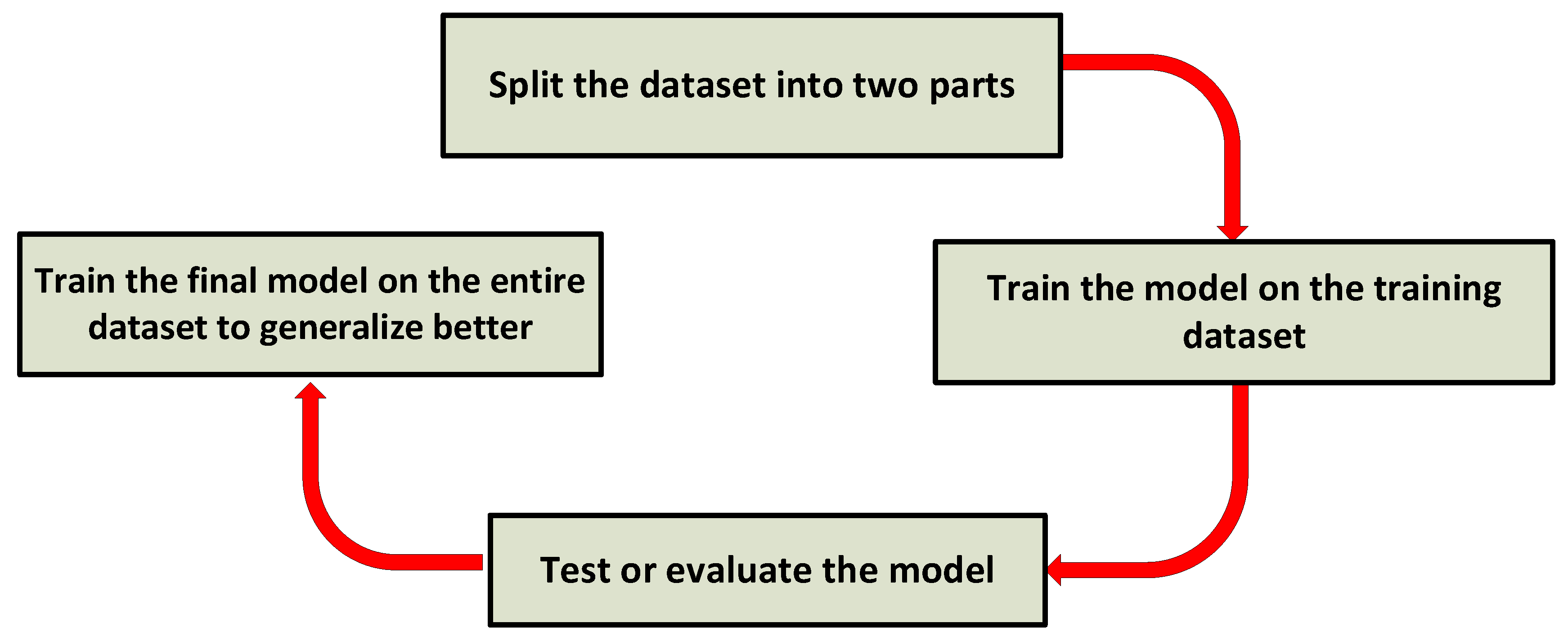
A common option for evaluating machine learning models is cross-validation. Cross-validation is a valuable method to evaluate how the results of a statistical examination could be generalized to an independent dataset. The main aim of the cross-validation approach is to determine a dataset to examine the model in the training phase for validation. This approach should be performed to reduce some problems such as overfitting. In this study, hold-out cross-validation is applied. The available data is divided into training and test/validation parts in the hold-out method to get the most optimal model. The model should be trained on the training dataset and assess on the test/validation dataset. The model evaluation techniques should be applied to validate the dataset to calculate the errors. The flowchart are shown in Figure 2. The flowchart of each cycle modeling is illustrated in Figure 3.
3. Results
After applying the curve fitting tool and optimizing the generated models and coefficients to reduce the errors, the most compatible correlation is obtained. It has been tried to generate the most reliable cost models according to the available cost results; however, the deviation in different models and parameters is different. Among the evaluated configurations, the regenerative ORC cycle had the highest deviation and scattered points. Additionally, among considered cost parameters, power generation cost had the highest deviation, so that for ORC cycles, these deviation is higher than flash cycles. The average tolerance of cost estimation of whole models is around 20%. This tolerance for ORC cycles mainly depends on working conditions and main operational parameters and the effect of working fluid on the main working condition and parameters of the system. However, this tolerance for flash cycles is less than ORCs as the working fluid is the same for all of them.
The hold-out validation can have different percentages of data being held out for examination [50]. In this study, 20% of all data are separated to validate other 80% cost data. It has been done to investigate how much the remained cost data (20%) are close to the generated fitting line. The statistical values of cost parameters and relevant design variables are presented in Table 3. The generated cost models and relevant coefficients for all considered configurations are brought in Table 4, Table 5 and Table 6. The R-square value related to each correlation is presented too that for all configurations expect regenerative ORC is higher than 90%. The cost data showed that these data are more scattered for regenerative ORC, increasing the error probability in model estimations. For flash cycles, three options are proposed, estimation of the cost models based on heat exchanger’s area and net power, heat exchanger’s area and volumetric flow of cooling tower fluid and net power, and cooling tower fluid’s volumetric flow. The cooling tower plays the main role in flash cycles’ total cost, and the only area value is related to the condenser. This parameter is considered separately as a design variable. The examination of cost models showed that all three offered options for flash cycles estimated the cost models with little difference.
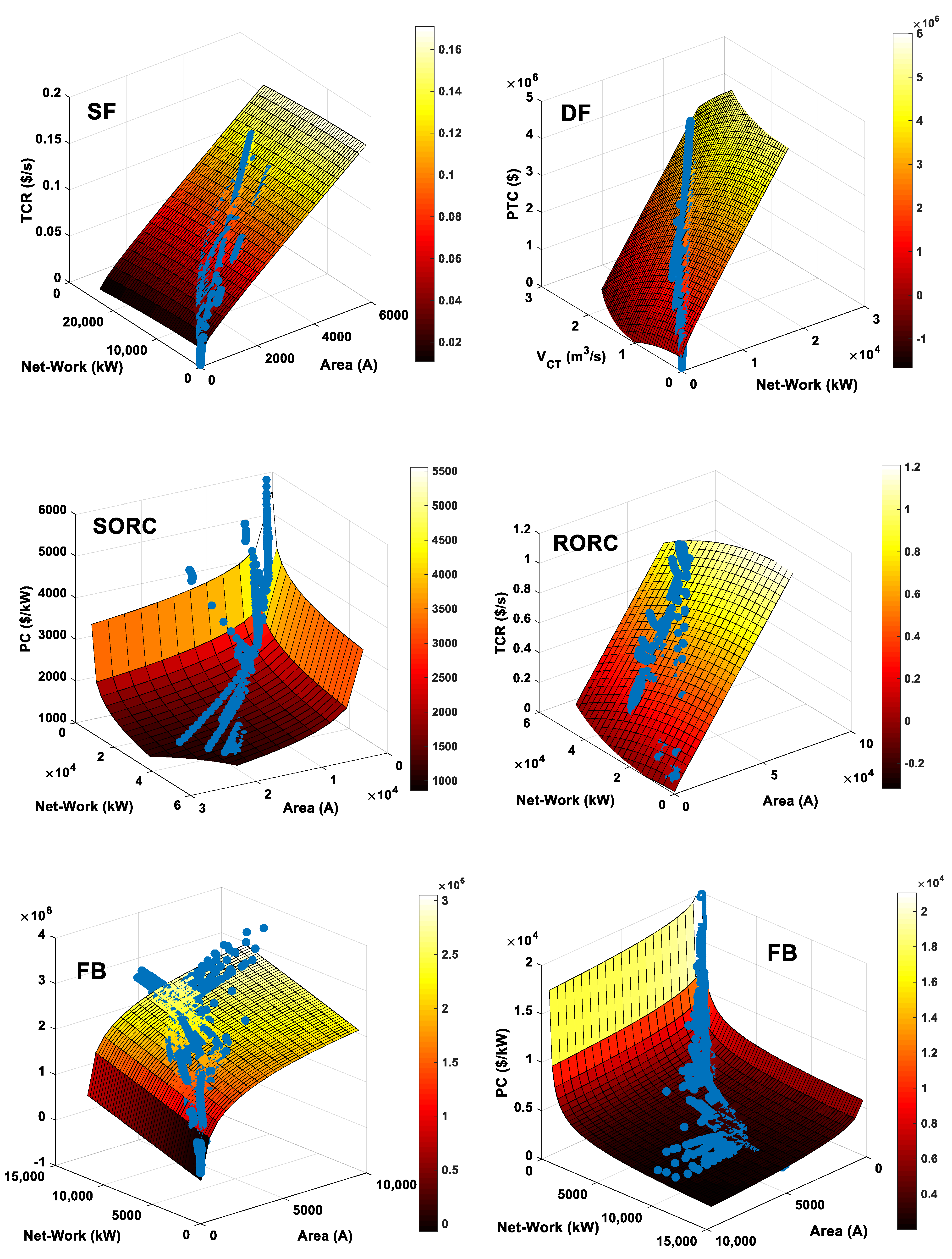
In addition, the fitting diagrams with some data for different configurations are shown in Figure 4. This fitting validation is performed using the remained examination data to determine how much the presented fitting model matches the data. According to the results obtained, the generated fitting surfaces present good compatibility with cost data. The proposed cost models in this study have several advantages. First, the generated models are related to the 2020 database (the most updated cost correlation applied), which means they are the most recently updated models for estimating the power plant cost. Most significantly, the benefit of this work is in applying optimization methods after generating the cost correlations and relevant coefficients. These models are presented for the different geothermal power cycles.
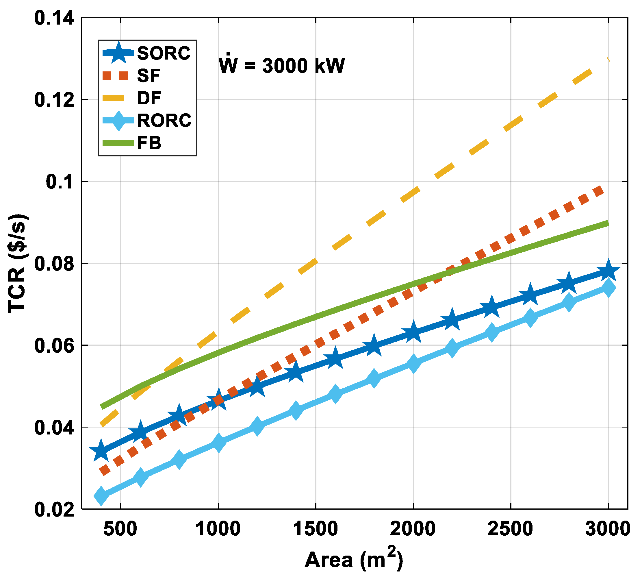
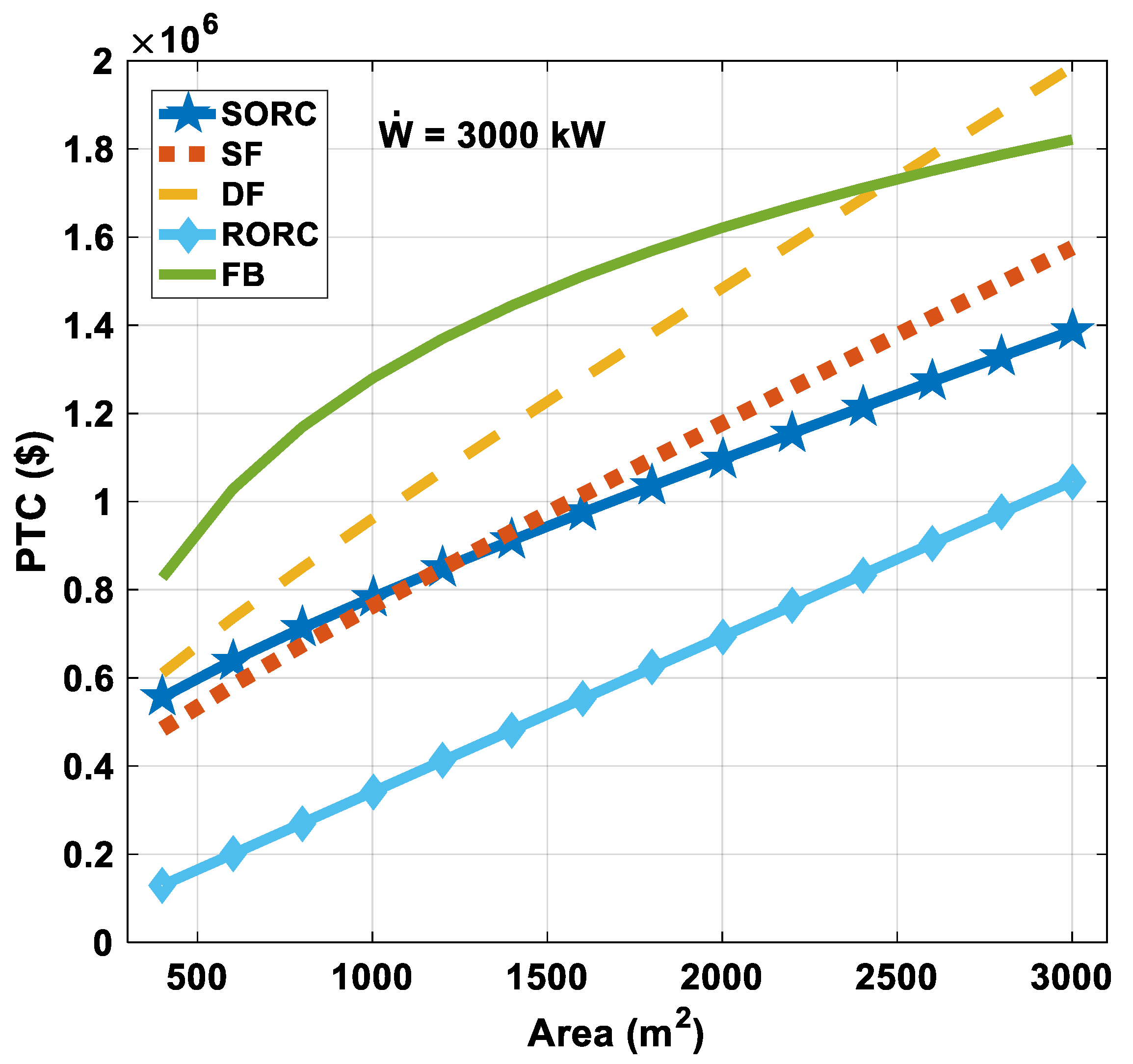
Additionally, the trends of cost models of different configurations for net power of 3000 kW based on the total area of heat exchangers variations are illustrated in Figure 5 and Figure 6. According to the results, increasing the total cost rate of double flash has occurred with the highest rate than others. Single flash has the second growing rate after double flash. Furthermore, the changing pattern of the single flash and simple ORC cycles for 400 to 3000 square meters stands close. The regenerative ORC has the lowest plant total cost among the cycles, mainly due to reduced condenser area by adding a regenerator and consequently a condenser with lower capacity. These trends present the differences in cost models based on just one dependent variable (heat exchanger’s area); however, estimating both dependent variables more accurately should be applied with cost models.
In order to validate the modeling, the obtained results were compared with other studies that showed good compatibility of our model with them which are presented in Table 7. In a parametric study [51], it has been proved that the maximum power of a single flash cycle could be obtained when the working temperature of the separator is the mean of condenser and geofluid temperatures. The present study has investigated that the optimal energy or exergy point is not necessarily economically viable.
4. Discussion
This study considers several operational parameters and main elements that may impact the selected cost functions. It has been concluded that two main parameters (net power and heat exchangers’ area) have the most significant impact on the economic results as they directly affect the equipment purchasing costs. Net power arising from the turbine, pump, compressor, etc., and heat exchangers area is one of the main parameters in determining equipment capacity. Then, these two factors play the most vital role in the economic evaluation of the power plant. In addition, for flash cycle cases, it has been found that cooling towers could be another dominant element in final cost assessments. In addition to the two previous options, this element has been considered for generating cost models. The cost models in this study have been divided and presented based on the different geothermal plants and configurations to reduce the deviation of their application. That is why it has been avoided to present just a single cost correlation for all configurations. The generated economic models and their relevant coefficient is calibrated carefully by two practical approaches. The methodology and model presented in this study followed an optimization method to reach the maximum reliability of model compatibility with data. The cross-validation approach, in addition to the optimization algorithm, has enhanced the capability of the generated models. Researchers could assess these configurations based on the first and second thermodynamic laws and quickly implement the generated economic models to find the results without spending too much time on exergo-economic modeling and writing code in the programming software. The studied geothermal cycles are the most common configurations. These economic models could be applied for the geothermal cycle integrating with other systems by adding the obtained economic results from the ORC or flash part of the system with other coupled systems.
5. Conclusions
The present study derived the models based on robust multivariable regression to minimize the residuals using the genetic algorithm. The cross-validation approach is applied to determine a dataset to examine the model in the training phase for validation and reduce the overfitting problem. According to the results obtained, the deviation in various models and parameters is different. Among the evaluated configurations, the regenerative ORC cycle had the highest deviation and scattered points. One of the main influential factors on economic results in ORC cycles is the working fluid type. Based on the model generation results, the working fluid could affect economic results significantly. In addition, as the critical pressure and temperature of various working fluids differ widely, the input parameters for thermodynamic modeling should be compatible with those values. Another effective parameter is the thermodynamic properties of the geothermal fluid, and after that, turbine inlet pressure and temperature were the most dominant parameter on the final obtained results. These elements lead to more deviation for the ORC cycle than flash technology. Additionally, among considered cost parameters, power generation cost had the highest deviation, so that for ORC cycles, these deviation is higher than flash cycles. Power cost can be affected by several parameters such as net generated power and equipment costs, leading to considerable changes in power generation cost. Among these cycles, flash-binary has the most significant power cost reduction with increasing the electricity generation capacity of the cycle. However, increasing the power generation capacity increases the investment cost at a higher rate than other cycles for the double flash cycle. The generated cost models are related to the 2020 database (the most updated cost correlation applied), which means they are the most recently updated models for estimating the power plant cost. Most significantly, the benefit of this work is in applying optimization methods after generating the cost correlations and relevant coefficients. The generated models are the robust cost models that can help researchers and stakeholders to estimate the economic parameters of the geothermal power plants.
Future recommendation: According to the results obtained in the present study, it is recommended that researchers should make a normalized balance between the power production and capacity of the equipment. This can be achieved by optimizing the process, selecting critical design variables such as the inlet and outlet condition of the heat exchanger, and selecting an excellent working fluid (for ORC) compatible with the economic performance of the cycle.
Author Contributions
Conceptualization, M.S., L.T. and P.H.N.; methodology, M.S., L.T. and P.H.N.; software, M.S.; validation, P.H.N. and L.T.; formal analysis, M.S.; investigation, M.S.; data curation, P.H.N. and L.T.; writing—original draft preparation, M.S.; writing—review and editing, P.H.N. and L.T.; supervision, G.M. and D.F.; project administration, G.M. and D.F. All authors have read and agreed to the published version of the manuscript.
Funding
This research received no external funding.
Institutional Review Board Statement
Not applicable.
Informed Consent Statement
Not applicable.
Data Availability Statement
Not applicable.
Conflicts of Interest
The authors declare no conflict of interest.
Appendix A

Table A1.
Main input values related to the cycles’ simulations.
| Parameter | Unit | Cycle Type | ||||
|---|---|---|---|---|---|---|
| SORC | SF | DF | RORC | FB | ||
| Ambient temperature | K | 298 | 298 | 298 | 298 | 298 |
| Ambient pressure | kpa | 101.3 | 101.3 | 101.3 | 101.3 | 101.3 |
| Production well temperature | K | 453 | 230 | 230 | 453 | 230 |
| Production well pressure | kpa | 1000 | 2800 | 2800 | 1000 | 2800 |
| Geofluid mass flow rate | kg/s | 50 | 50 | 50 | 50 | 50 |
| Production well temperature | K | 363 | 363 | 323 | 363 | 333 |
| Turbine isentropic efficiencies | % | 80 | 80 | 80 | 80 | 80 |
| Pump isentropic efficiencies | % | 85 | 85 | 85 | 85 | 85 |
| Regenerator isentropic efficiencies | % | - | - | - | 80 | 80 |
| Inlet pressure of ORC turbine | kpa | 3130 | - | - | 3130 | - |
| Pressure after HP EV | kpa | - | 276 | 665 | - | 400 |
| Pressure after LP EV | kpa | - | - | 96 | - | - |
| Heat transfer coefficients of HXs | kW/m2K | 1.1 | 1.1 | 1.1 | 1.1 | 1.1 |
| Pinch point of HXs | K | 10 | 10 | 10 | 10 | 10 |
| Quality of pump inlet fluid | - | 0 | - | - | 0 | 0 |
| Inlet cold fluid temperature of condenser | K | 298 | 298 | 298 | 298 | 298 |
| Outlet cold fluid temperature of condenser | K | 308 | 308 | 308 | 308 | 308 |
| ORC working fluid | - | R1233ZD | - | - | R1233ZD | R1233ZD |
Nomenclature
| Area of heat exchanger, m2 | |
| Specific exergy cost, $/kJ | |
| Cost rate associated with exergy transfer, $/s | |
| Chemical Engineering Plant Cost Index | |
| Condenser | |
| Capital Recovery Factor | |
| Double Flash | |
| Specific exergy, kJ/kg | |
| Exergy rate, kW | |
| Expansion valve | |
| Evaporator | |
| Flash-Binary | |
| Generator | |
| Specific enthalpy, kJ/kg | |
| Heat exchanger | |
| Rate of interest | |
| logarithmic mean temperature difference | |
| Mass flow rate, kg/s | |
| Annual plant operation hours | |
| Organic Rankine cycle | |
| Pump | |
| Power cost, $/ kW | |
| Plant Total Cost, ($) | |
| Heat transfer rate, kW | |
| Regenerator | |
| Regenerative ORC | |
| Specific entropy, kJ/Kgk | |
| Separator | |
| Single Flash | |
| Simple ORC | |
| Temperature, (K) | |
| Total capital investment, ($) | |
| Total Cost Rate, $/s | |
| Heat transfer coefficient, W/Km2 | |
| Intensity of the flow, m3/s | |
| Power, kW | |
| Capital cost of components, ($) | |
| Capital cost rate of components, $/s | |
| Greek Symbols | |
| Maintenance factor | |
| Efficiency, | |
| Subscripts | |
| Cooling Tower | |
| Destruction | |
| Exit | |
| Fuel | |
| Inlet | |
| Product | |
| Ambient | |
References
- Torp, O.; Klakegg, O.J. Challenges in cost estimation under uncertainty—A case study of the decommissioning of Barsebäck Nuclear Power Plant. Adm. Sci. 2016, 6, 14. [Google Scholar] [CrossRef] [Green Version]
- Turton, R.; Bailie, R.C.; Whiting, W.B.; Shaeiwitz, J.A. Analysis, Synthesis and Design of Chemical Processes; Pearson Education: London, UK, 2008. [Google Scholar]
- Ahmadi, A.; El Haj Assad, M.; Jamali, D.H.; Kumar, R.; Li, Z.X.; Salameh, T.; Al-Shabi, M.; Ehyaei, M.A. Applications of geothermal organic Rankine Cycle for electricity production. J. Clean. Prod. 2020, 274, 122950. [Google Scholar] [CrossRef]
- Leveni, M.; Cozzolino, R. Energy, exergy, and cost comparison of Goswami cycle and cascade organic Rankine cycle/absorption chiller system for geothermal application. Energy Convers. Manag. 2021, 227, 113598. [Google Scholar] [CrossRef]
- Loni, R.; Mahian, O.; Najafi, G.; Sahin, A.Z.; Rajaee, F.; Kasaeian, A.; Mehrpooya, M.; Bellos, E.; le Roux, W.G. A critical review of power generation using geothermal-driven organic Rankine cycle. Therm. Sci. Eng. Prog. 2021, 25, 101028. [Google Scholar] [CrossRef]
- Rudiyanto, B.; Bahthiyar, M.A.; Pambudi, N.A.; Hijriawan, M. An update of second law analysis and optimization of a single-flash geothermal power plant in Dieng, Indonesia. Geothermics 2021, 96, 102212. [Google Scholar] [CrossRef]
- Cao, Y.; Ehyaei, M.A. Energy, exergy, exergoenvironmental, and economic assessments of the multigeneration system powered by geothermal energy. J. Clean. Prod. 2021, 313, 127823. [Google Scholar] [CrossRef]
- El Haj Assad, M.; Khosravi, A.; Nazari, M.A.; Rosen, M.A. Chapter 10—Geothermal power plants. In Design and Performance Optimization of Renewable Energy Systems; Assad, M.E.H., Rosen, M.A., Eds.; Academic Press: Cambridge, MA, USA, 2021; pp. 147–162. [Google Scholar]
- Dincer, I.; Rosen, M.A. Chapter 11—Exergy analyses of renewable energy systems. In Exergy, 3rd ed.; Dincer, I., Rosen, M.A., Eds.; Elsevier: Amsterdam, The Netherlands, 2021; pp. 241–324. [Google Scholar]
- Williams, R. Six-tenths factor aids in approximating costs. Chem. Eng. 1947, 54, 124–125. [Google Scholar]
- Hamilton, A.C.; Westney, R.E. Cost estimating best practices. AACE Int. Trans. 2002, ES21. Available online: http://0-search-ebscohost-com.brum.beds.ac.uk/login.aspx?direct=true&db=buh&AN=7197098&site=ehost-live (accessed on 18 April 2021).
- Max, S.P.; Klaus, D.T.; Ronald, E.W. Plant Design and Economics for Chemical Engineers; McGraw-Hill Companies: New York, NY, USA, 2003. [Google Scholar]
- Yang, I.-T. Simulation-based estimation for correlated cost elements. Int. J. Proj. Manag. 2005, 23, 275–282. [Google Scholar] [CrossRef]
- Caputo, A.C.; Pelagagge, P.M. Parametric and neural methods for cost estimation of process vessels. Int. J. Prod. Econ. 2008, 112, 934–954. [Google Scholar] [CrossRef]
- Blankenship, D.A.; Mansure, A. Geothermal Well Cost Analyses 2008; Sandia National Lab. (SNL-NM): Albuquerque, NM, USA, 2008. [Google Scholar]
- Ogayar, B.; Vidal, P. Cost determination of the electro-mechanical equipment of a small hydro-power plant. Renew. Energy 2009, 34, 6–13. [Google Scholar] [CrossRef]
- Feng, Y.; Rangaiah, G.P. Evaluating capital cost estimation programs. Chem. Eng. 2011, 118, 22–29. [Google Scholar]
- Brotherson, W.T.; Eades, K.M.; Harris, R.S.; Higgins, R.C. ‘Best Practices’ in Estimating the Cost of Capital: An Update. J. Appl. Financ. (Former. Financ. Pract. Educ.) 2013, 23. Available online: https://ssrn.com/abstract=2686738 (accessed on 15 May 2021).
- Gunduz, M.; Sahin, H.B. An early cost estimation model for hydroelectric power plant projects using neural networks and multiple regression analysis. J. Civ. Eng. Manag. 2015, 21, 470–477. [Google Scholar] [CrossRef]
- Symister, O.J. An Analysis of Capital Cost Estimation Techniques for Chemical Processing. Master’s Thesis, Florida Institute of Technology, Melbourne, FL, USA, May 2016. [Google Scholar]
- Caputo, A.C.; Pelagagge, P.M.; Salini, P. Manufacturing cost model for heat exchangers optimization. Appl. Therm. Eng. 2016, 94, 513–533. [Google Scholar] [CrossRef]
- Luyben, W.L. Capital cost of compressors for conceptual design. Chem. Eng. Process. Process. Intensif. 2018, 126, 206–209. [Google Scholar] [CrossRef]
- Gul, S.; Aslanoglu, V. Drilling and Well Completion Cost Analysis of Geothermal Wells in Turkey. In Proceedings of the 43rd Workshop on Geothermal Reservoir Engineering, Stanford, CA, USA, 12–14 February 2018. [Google Scholar]
- Amorim, D.S., Jr.; Santos, O.L.A.; de Azevedo, R.C. A statistical solution for cost estimation in oil well drilling. REM-Int. Eng. J. 2019, 72, 675–683. [Google Scholar] [CrossRef]
- Malhan, P.; Mittal, M. Evaluation of different statistical techniques for developing cost correlations of micro hydro power plants. Sustain. Energy Technol. Assess. 2021, 43, 100904. [Google Scholar]
- Shamoushaki, M.; Niknam, P.H.; Talluri, L.; Manfrida, G.; Fiaschi, D. Development of Cost Correlations for the Economic Assessment of Power Plant Equipment. Energies 2021, 14, 2665. [Google Scholar] [CrossRef]
- Shamoushaki, M.; Fiaschi, D.; Manfrida, G.; Niknam, P.H.; Talluri, L. Feasibility study and economic analysis of geothermal well drilling. Int. J. Environ. Stud. 2021, 1–15. [Google Scholar] [CrossRef]
- NIST Standard Reference Database 23. NIST Thermodynamic and Transport Properties of Refrigerants and Refrigerant Mixtures REFPROP, 2013; Version 9.1; NIST: Gaithersburg, MD, USA, 2013. [Google Scholar]
- Chemical Engineering Plant Cost Index. Available online: https://www.chemengonline.com/pci-home (accessed on 22 July 2021).
- Bejan, A.; Tsatsaronis, G.; Moran, M. Thermal Design and Optimization; John Wiley and Sons. Inc.: New York, NY, USA, 1996. [Google Scholar]
- DiPippo, R. Geothermal Power Plants: Principles, Applications, Case Studies and Environmental Impact; Butterworth-Heinemann: Oxford, UK, 2012. [Google Scholar]
- Lazzaretto, A.; Tsatsaronis, G. SPECO: A systematic and general methodology for calculating efficiencies and costs in thermal systems. Energy 2006, 31, 1257–1289. [Google Scholar] [CrossRef]
- Boyaghchi, F.A.; Chavoshi, M. Multi-criteria optimization of a micro solar-geothermal CCHP system applying water/CuO nanofluid based on exergy, exergoeconomic and exergoenvironmental concepts. Appl. Therm. Eng. 2017, 112, 660–675. [Google Scholar] [CrossRef]
- Fiaschi, D.; Manfrida, G.; Rogai, E.; Talluri, L. Exergoeconomic analysis and comparison between ORC and Kalina cycles to exploit low and medium-high temperature heat from two different geothermal sites. Energy Convers. Manag. 2017, 154, 503–516. [Google Scholar] [CrossRef]
- Shamoushaki, M.; Ehyaei, M.; Ghanatir, F. Exergy, economic and environmental analysis and multi-objective optimization of a SOFC-GT power plant. Energy 2017, 134, 515–531. [Google Scholar] [CrossRef]
- Shamoushaki, M.; Ehyaei, M.A. Exergy, economic and environmental (3E) analysis of a gas turbine power plant and optimization by MOPSO algorithm. Therm. Sci. 2018, 22, 2641–2651. [Google Scholar] [CrossRef] [Green Version]
- Akrami, E.; Chitsaz, A.; Nami, H.; Mahmoudi, S. Energetic and exergoeconomic assessment of a multi-generation energy system based on indirect use of geothermal energy. Energy 2017, 124, 625–639. [Google Scholar] [CrossRef]
- Ehyaei, M.; Ahmadi, A.; Assad, M.E.H.; Rosen, M.A. Investigation of an integrated system combining an Organic Rankine Cycle and absorption chiller driven by geothermal energy: Energy, exergy, and economic analyses and optimization. J. Clean. Prod. 2020, 258, 120780. [Google Scholar] [CrossRef]
- Fiaschi, D.; Manfrida, G.; Mendecka, B.; Shamoushaki, M.; Talluri, L. Exergy and Exergo-Environmental Analysis of an ORC for a Geothermal Application. E3S Web Conf. 2021, 238, 01011. [Google Scholar] [CrossRef]
- Mohammadkhani, F.; Shokati, N.; Mahmoudi, S.; Yari, M.; Rosen, M. Exergoeconomic assessment and parametric study of a Gas Turbine-Modular Helium Reactor combined with two Organic Rankine Cycles. Energy 2014, 65, 533–543. [Google Scholar] [CrossRef]
- Shamoushaki, M.; Ghanatir, F.; Ehyaei, M.; Ahmadi, A. Exergy and exergoeconomic analysis and multi-objective optimisation of gas turbine power plant by evolutionary algorithms. Case study: Aliabad Katoul power plant. Int. J. Exergy 2017, 22, 279–307. [Google Scholar] [CrossRef]
- Zoghi, M.; Habibi, H.; Chitsaz, A.; Javaherdeh, K.; Ayazpour, M. Exergoeconomic analysis of a novel trigeneration system based on organic quadrilateral cycle integrated with cascade absorption-compression system for waste heat recovery. Energy Convers. Manag. 2019, 198, 111818. [Google Scholar] [CrossRef]
- Nourani, Z.; Naserbegi, A.; Tayyebi, S.; Aghaie, M. Thermodynamic evaluation of hybrid cooling towers based on ambient temperature. Therm. Sci. Eng. Prog. 2019, 14, 100406. [Google Scholar] [CrossRef]
- Mosaffa, A.; Farshi, L.G.; Ferreira, C.I.; Rosen, M. Exergoeconomic and environmental analyses of CO2/NH3 cascade refrigeration systems equipped with different types of flash tank intercoolers. Energy Convers. Manag. 2016, 117, 442–453. [Google Scholar] [CrossRef] [Green Version]
- Ghasemian, E.; Ehyaei, M. Evaluation and optimization of organic Rankine cycle (ORC) with algorithms NSGA-II, MOPSO, and MOEA for eight coolant fluids. Int. J. Energy Environ. Eng. 2018, 9, 39–57. [Google Scholar] [CrossRef] [Green Version]
- Shamoushaki, M.; Ehyaei, M. Optimization of gas turbine power plant by evoloutionary algorithm; considering exergy, economic and environmental aspects. J. Therm. Eng. 2020, 6, 180–200. [Google Scholar] [CrossRef]
- Roetzel, W.; Luo, X.; Chen, D. Optimal design of heat exchanger networks. In Design and Operation of Heat Exchangers and Their Networks; Elsevier: Amsterdam, The Netherlands, 2019; pp. 231–318. [Google Scholar]
- Niknam, P.H.; Talluri, L.; Fiaschi, D.; Manfrida, G. Improved Solubility Model for Pure Gas and Binary Mixture of CO2-H2S in Water: A Geothermal Case Study with Total Reinjection. Energies 2020, 13, 2883. [Google Scholar] [CrossRef]
- Koul, A.; Becchio, C.; Cavallo, A. Cross-validation approaches for replicability in psychology. Front. Psychol. 2018, 9, 1117. [Google Scholar] [CrossRef] [PubMed]
- Yadav, S.; Shukla, S. Analysis of k-fold cross-validation over hold-out validation on colossal datasets for quality classification. In Proceedings of the 2016 IEEE 6th International conference on advanced computing (IACC), Bhimavaram, India, 27–28 February 2016; IEEE: Piscataway, NJ, USA, 2016; pp. 78–83. [Google Scholar]
- Assad, M.E.H.; Aryanfar, Y.; Radman, S.; Yousef, B.; Pakatchian, M. Energy and exergy analyses of single flash geothermal power plant at optimum separator temperature. Int. J. Low Carbon. Technol. 2021. [Google Scholar] [CrossRef]
- Shokati, N.; Ranjbar, F.; Yari, M. Comparative and parametric study of double flash and single flash/ORC combined cycles based on exergoeconomic criteria. Appl. Therm. Eng. 2015, 91, 479–495. [Google Scholar] [CrossRef]
- Zare, V. A comparative exergoeconomic analysis of different ORC configurations for binary geothermal power plants. Energy Convers. Manag. 2015, 105, 127–138. [Google Scholar] [CrossRef]
- Mohammadzadeh Bina, S.; Jalilinasrabady, S.; Fujii, H. Exergoeconomic analysis and optimization of single and double flash cycles for Sabalan geothermal power plant. Geothermics 2018, 72, 74–82. [Google Scholar] [CrossRef]
Figure 1.
Flowchart of the genetic algorithm.

Figure 2.
Flowchart of cross-validation process.

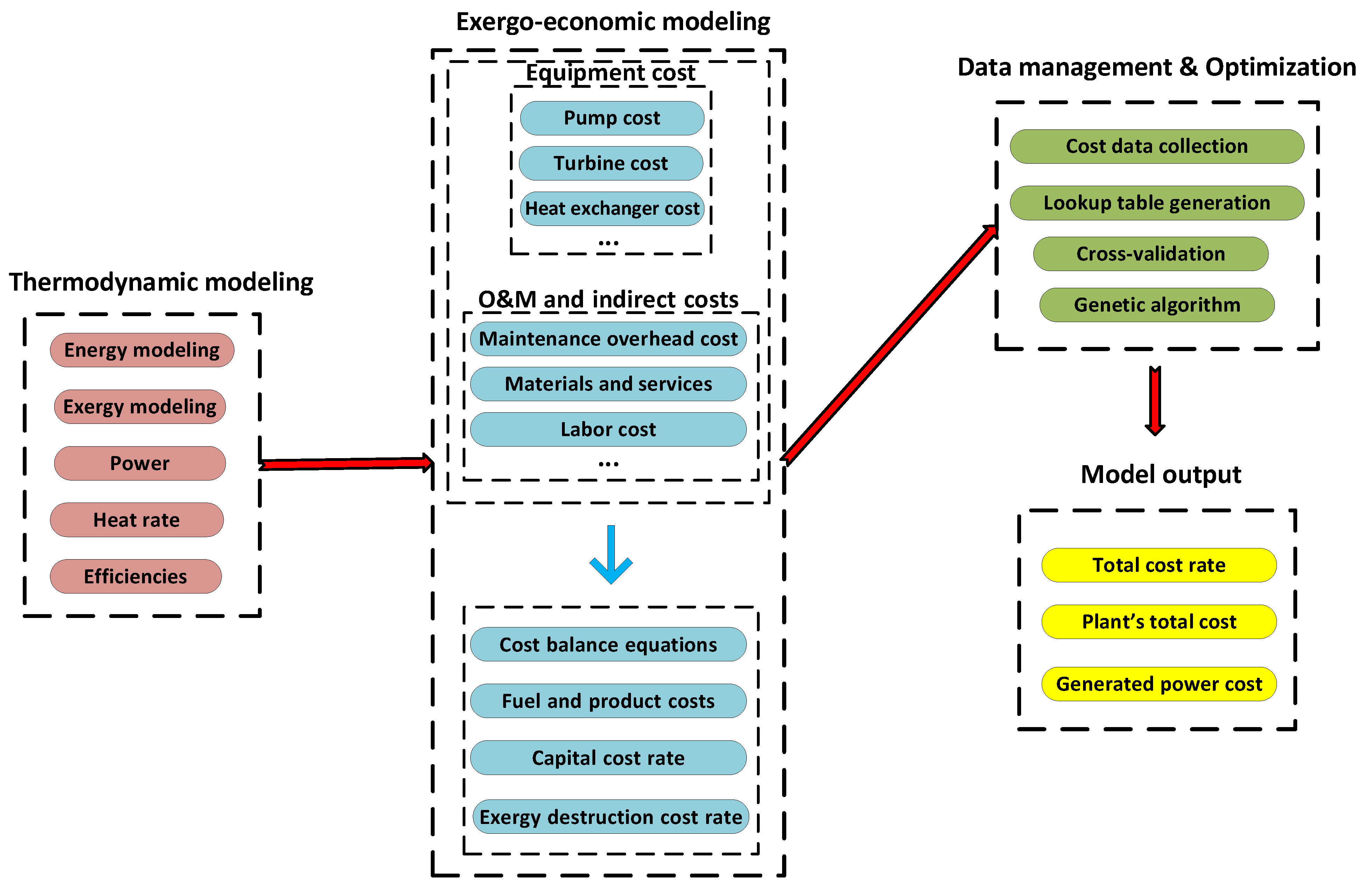
Figure 3.
Flowchart of cycles modeling.

Figure 4.
Fitting graphs with some data for different configurations.

Figure 5.
TCR trend against heat exchanger area at net power of 3000 kW.

Figure 6.
PTC trend against heat exchanger area at net power of 3000 kW.

Table 1.
The equipment purchasing cost correlations.
| Component | Cost Correlation | Coefficients | Ref. |
|---|---|---|---|
| Pump | [26] | ||
| Turbine | [2] | ||
| HEs | [26] | ||
| EV | - | [42] | |
| Cond | [26] | ||
| CT | [43] | ||
| Sep | - | [44] | |
| Gen | - | [45] |
Table 2.
Input parameters applied in thermodynamic modeling.
| Parameter | SORC | SF | DF | RORC | FB |
|---|---|---|---|---|---|
| Ambient temperature | ✔ | ✔ | ✔ | ✔ | ✔ |
| Ambient pressure | ✔ | ✔ | ✔ | ✔ | ✔ |
| Turbine Inlet pressure | ✔ | ✔ | ✔ | ✔ | ✔ |
| Quality of pump inlet | ✔ | ✔ | ✔ | ||
| Working fluid selection | ✔ | ✔ | ✔ | ||
| EV pressure ratio | ✔ | ✔ | ✔ | ||
| PW pressure | ✔ | ✔ | ✔ | ✔ | ✔ |
| PW temperature | ✔ | ✔ | ✔ | ✔ | ✔ |
| Efficiency of turbine | ✔ | ✔ | ✔ | ✔ | ✔ |
| Efficiency of pump | ✔ | ✔ | ✔ | ||
| Geofluid mass flow rate | ✔ | ✔ | ✔ | ✔ | ✔ |
| Cold fluid temperature of condenser | ✔ | ✔ | ✔ | ✔ | ✔ |
Table 3.
Statistical parameters of all considered configurations.
| Cycle Type | Parameter | Number of Data | Mean | Median | Standard Deviation | Confidence Interval |
|---|---|---|---|---|---|---|
| SORC | Area (m2) | 3550 | 4274.2 | 3991.9 | 3808.6 | 2.9% |
| Net work (kW) | 3550 | 8525.1 | 6855.8 | 6848.4 | 2.6% | |
| TCR (S/s) | 3550 | 0.0910 | 0.0878 | 0.0463 | 1.7% | |
| PTC ($) | 3550 | 1,664,026.5 | 1,627,391.4 | 936,843.8 | 1.9% | |
| PC (S/kW) | 3550 | 2465.4 | 2405.5 | 896.6 | 1.2% | |
| SF | Area (m2) | 1550 | 1164.9 | 699.5 | 1280.1 | 5.5% |
| Net work (kW) | 1550 | 2407.1 | 1594.1 | 2499.2 | 5.2% | |
| VCT (m3/s) | 1550 | 0.279 | 0.168 | 0.307 | 5.5% | |
| TCR (S/s) | 1550 | 0.0474 | 0.0384 | 0.0356 | 3.7% | |
| PTC ($) | 1550 | 751,877.5 | 713,788.4 | 556,478.1 | 3.7% | |
| PC (S/kW) | 1550 | 8912.9 | 4563.6 | 7482.8 | 4.2% | |
| DF | Area (m2) | 2750 | 2606.5 | 2220.2 | 2307 | 3.3% |
| Net work (kW) | 2750 | 5378.2 | 4445.7 | 4994.5 | 3.5% | |
| VCT (m3/s) | 2750 | 0.6252 | 0.5326 | 0.5534 | 3.3% | |
| TCR (S/s) | 2750 | 0.1068 | 0.1057 | 0.0699 | 2.4% | |
| PTC ($) | 2750 | 1,615,940.5 | 1,664,920.2 | 1,079,097.1 | 2.5% | |
| PC (S/kW) | 2750 | 7550.4 | 4155.4 | 6276.1 | 3.1% | |
| RORC | Area (m2) | 4115 | 16,775.1 | 12,158.6 | 13,312.2 | 2.4% |
| Net work (kW) | 4115 | 16,596.7 | 12,972.1 | 12,368.1 | 2.3% | |
| TCR (S/s) | 4115 | 0.2519 | 0.1696 | 0.2279 | 2.8% | |
| PTC ($) | 4115 | 5,094,807.1 | 3,375,450.1 | 4,794,940.1 | 2.9% | |
| PC (S/kW) | 4115 | 3182.9 | 3002.1 | 1144.2 | 1.1% | |
| FB | Area (m2) | 7450 | 1730.9 | 1327.8 | 1578.1 | 2.1% |
| Net work (kW) | 7450 | 3700.1 | 2716.9 | 3487.1 | 2.1% | |
| TCR (S/s) | 7450 | 0.0690 | 0.0669 | 0.0346 | 1.1% | |
| PTC ($) | 7450 | 1,364,011.6 | 1,350,956.2 | 762,586 | 1.3% | |
| PC (S/kW) | 7450 | 7563 | 5512.5 | 5513.2 | 1.7% |
Table 4.
Total Cost Rate model (TCR) for all configurations.
| Cycle | Correlation | ||||
|---|---|---|---|---|---|
| SORC | |||||
| SF | |||||
| DF | |||||
| RORC | |||||
| FB |
Table 5.
Plant total cost models (PTC) for all configurations.
| Cycle | Correlation | ||||
|---|---|---|---|---|---|
| SORC | |||||
| SF | |||||
| DF | |||||
| RORC | |||||
| FB |
Table 6.
Power cost (PC) for all configurations.
| Cycle | Correlation | ||||
|---|---|---|---|---|---|
| SORC | |||||
| SF | |||||
| DF | |||||
| RORC | |||||
| FB |
| Parameter | Unit | Geothermal Cycle Type | Ref Value | Present Study | |
|---|---|---|---|---|---|
| TCR | $/s | DF | 0.008 | 0.0078 | −2.5 |
| TCR | $/s | FB | 0.0181 | 0.0201 | +11 |
| TCR | $/s | FB | 0.0215 | 0.0236 | +9.7 |
| PC | $/ kW | SORC | 1687 | 1723 | +2.1 |
| PC | $/ kW | SORC | 1341 | 1399 | +4.3 |
| PC | $/ kW | RORC | 1847 | 1957 | +5.9 |
| PC | $/ kW | RORC | 1615 | 1711 | +5.9 |
| PTC | $ | SF | 3.27 × 10⁶ | 3.02 × 10⁶ | −7.6 |
| PTC | $ | DF | 9.97 × 10⁶ | 1.04 × 10⁷ | +4.3 |
Publisher’s Note: MDPI stays neutral with regard to jurisdictional claims in published maps and institutional affiliations. |
© 2021 by the authors. Licensee MDPI, Basel, Switzerland. This article is an open access article distributed under the terms and conditions of the Creative Commons Attribution (CC BY) license (https://creativecommons.org/licenses/by/4.0/).
Share and Cite
MDPI and ACS Style
Shamoushaki, M.; Manfrida, G.; Talluri, L.; Niknam, P.H.; Fiaschi, D. Different Geothermal Power Cycle Configurations Cost Estimation Models. Sustainability 2021, 13, 11133. https://0-doi-org.brum.beds.ac.uk/10.3390/su132011133
AMA Style
Shamoushaki M, Manfrida G, Talluri L, Niknam PH, Fiaschi D. Different Geothermal Power Cycle Configurations Cost Estimation Models. Sustainability. 2021; 13(20):11133. https://0-doi-org.brum.beds.ac.uk/10.3390/su132011133
Chicago/Turabian StyleShamoushaki, Moein, Giampaolo Manfrida, Lorenzo Talluri, Pouriya H. Niknam, and Daniele Fiaschi. 2021. "Different Geothermal Power Cycle Configurations Cost Estimation Models" Sustainability 13, no. 20: 11133. https://0-doi-org.brum.beds.ac.uk/10.3390/su132011133
Note that from the first issue of 2016, this journal uses article numbers instead of page numbers. See further details here.