An Optimization-Based System Dynamics Simulation for Sustainable Policy Design in WEEE Management Systems

Abstract

The increase in the use of electrical and electronic devices worldwide has created a rapid growth of waste of electrical and electronic equipment (WEEE). The current paper presents an optimization-based simulation (OBS) approach that allows the design of sustainable WEEE management system policies. The proposed OBS approach integrates a system dynamics (SD) model and a mixed-integer nonlinear programming (MINLP) model to improve the representation and performance of the WEEE processes considering their operative and strategic interdependence. The SD component elicits the complexity of the WEEE generation process. Complementarily, the MINLP model periodically optimizes key variables of the WEEE management system. Computational results in a case study based on WEEE from Colombian mobile phones illustrates how an approach solely based on SD simulation is unable to capture the operative-strategic nature of the system and perform optimal parameter updates. By contrast, the OBS approach of this paper outperforms an exclusive SD analysis both in the economic and environmental performance of the system. It obtains 33% more profits and 65% more environmental benefits. Moreover, for this case study, the model suggests that the cornerstone of the WEEE management system for increasing its performance is the replacement rate.

1. Introduction

Worldwide, there is an increasing trend toward the massive consumption of all electrical and electronic equipment (EEE) such as cell phones, tablets, smart televisions and computers [1]. The increase in EEE consumption has been accelerated by several factors such as international trade conditions, decreasing cost of products, the rise of social media and continuous technological innovations [1,2,3]. As a consequence, the EEE life cycles are shorter, the generation of waste of electrical and electronic equipment (WEEE) has increased over the past years, and it is expected that it will increase even more in the foreseeable future [1,4,5,6,7]. In 2016, estimations suggest that global WEEE exceeded 44 Megatons (Mt); however, by 2019, the amount was surpassing a value of nearly 53.6 Mt worldwide and is projected to reach 74.7 Mt by 2030 [2,8]. In China alone, it is expected that the growth of obsolete electronic devices would average 18% per year, where the growth rate of some items like air conditioners would increase at rates of near 40% annually [5,9].

While several (developed) countries have improved their WEEE management systems, WEEE management remains a challenge for almost all countries since only 20% of the total global WEEE is currently recycled [3,4,10,11]. The main difficulty lies in the establishment of a fully functional and integrated disposal management system that is able to process and benefit from the WEEE recovered [12,13]. In emerging countries, the lack of suited WEEE management systems is especially pressing because environmental and human health impacts are directly linked to the exposure of WEEE toxic materials [14,15,16,17]. Additionally, the WEEE recycling industry brings opportunities for new sources of employment and development [4,6,18].

To establish an integrated WEEE management system, it is necessary to consider its main stages: (i) product acquisition/gate keeping, (ii) collection, (iii) inspection and sorting and (iv) disposition [19]. Each of these stages are subject to be optimized in their design and performance [20]. That is why much of the literature on WEEE management systems has focused mainly on the optimization of one or two stages of the whole process [5,19,21,22]. However, there is the need of approaches that are able to address the coordination of these four stages in a scheme of integration capable of guaranteeing future and systemic performance [5,19,21,22]. Optimization techniques are ideal when the context of the problem is static, linear and deterministic, but as the modeling of the system incorporates time and nonlinear behavior, optimization techniques face limitations.

Given their capacity for eliciting complex systems nature, simulation techniques such as Discrete-Event Simulation (DES), System Dynamics (SD) and Agent-Based Simulation (ABS) are among the most used quantitative approaches. They are designed to understand the interaction between policy and behavior [23]. DES and ABS approaches are more commonly implemented to address problems whose nature is operative and detail-oriented [24]. Conversely, SD allows a strategic/tactical approach which is ideal for modeling the interaction of components in large systems [4,5,19,25]. Thus, all of them have been widely applied to improve the performance of either one or several WEEE management processes. However, the main use of SD and ABS simulation techniques is for the analysis of the process of generation and acquisition [26,27], while DES models are mainly used for modeling the processes of collection and disposition [28]. Overall, these methodologies are able to incorporate the stochastic and dynamic nature of the WEEE management systems and also target the analysis considering either the strategic or the operative nature of the problem [29,30].

In modeling the interaction of the four aforementioned process, most of the literature uses SD as a primary methodology given its versatility to elicit complex and large systems [25]. This is mainly due to the fact that SD modeling is well-suited for eliciting the effects of delays and feedbacks in the performance of interrelated variables describing complex behavior [23]. The works by [31,32] can be taken as examples of this. The first study analyzes the long-term behavior of a closed-loop supply chain with recycling activities under scenarios of ecological motivations and technological innovations. The second work evaluates the impact of regulations, activities, and practices on closed-loop supply chains measuring their environmental and economic performance. In analyzing the WEEE management dynamics in specific geographical contexts, the work by [33] uses SD to evaluate the impact of Chinese policies to promote WEEE recycling, while the work by [34] pursues a similar analysis in Latin America. In addressing WEEE management problems, SD has been used to model the whole system from an aggregated perspective [4,5,19,25]. This approach conveys a holistic analysis of the integration of the WEEE management system stages. As a result, the SD approach provides future performance scenarios of waste recovery and profit, given the policy decisions and the system structure [4,5,19,25,35].

In addition to the use of SD as a tool for operative or strategic planning, there is a recurrent topic of contributions addressing strategies to improve the recovery of WEEE. Consider, for instance, the work by [5], which assesses the role of the informal sector as a main contributor in the process of collection of used electric and electronic devices in India. The work by [36] uses an SD approach to explore the formalization of Brazilian waste pickers as a strategy for social empowerment and WEEE recolection. Similarly, the work by [37] develops a novel approach on the use of SD to determine policies for used mobile phone recycling in China. In the same context, [38] introduces an SD methodology to study the effects of retailer-led recycling of WEEE. The contribution by [4] introduces a mobile phone case study which explores the main determining factors influencing electronic waste generation in Colombia. A recent contribution addresses the mitigation of lead pollution due to recycling in India [25].

All these aforementioned contributions illustrate how the use of SD methodology is well established as a suited approach for guiding policy and strategy in WEEE management systems. However, there is the need of a new set of hybrid simulation models with the purpose of exploding the SD reach even further [39]. This is because SD as a methodology has some limitations that prevent the capture of WEE management systems’ more realistic behavior. The simulation approach rests upon the use of constants. It models state or decision variables whose change is assumed to be constant over the time horizon of interest [23]. This assumption constrains the use of SD to an aggregated representation of the WEEE managing systems, since tactical and operative processes require frequent updates of state and decisions variables. This updates need to convey the changes in products, process and market constrains [24]. Then, the use of SD to understand the behavior of the WEEE managing systems over time is prone to provide an unrealistic representation of the real behavior as the time horizon of interest is larger. Thus, by using an SD modeling, there is a limitation in capturing how operative and tactical decisions in the short run affect the overall performance of the system in the long run [24].

The WEEE management systems literature presents few examples of the integration of simulation and optimization as an approach to overcome the limitations of both methodologies. Consider, for instance, the work by [35], which implements an ABS model seeking to maximize the profit of a remanufacturing company. Similarly, [40] developed a DES simulation-based optimization model to determine the best locations for the collection centers and recycling plants for managing WEEE. The integration of SD and optimization for the improvement of WEEE management systems does not have examples that have been reported in the literature. However, the combination of both methodologies has been implemented in different fields as a complementary approach for policy analysis and systems design [41]. Dangerfield and Roberts [42] used optimization in SD as an approach to accomplish two main tasks: optimization to fit data and policy optimization to improve systems performance. In consequence, such efforts to integrate SD and optimization had produced a group of applications in several fields: coal industry [43], energy consumption [44] and water supply [45]. Our study argues that given the widespread use of SD in the improvement of WEEE management systems, there is a need to develop more research illustrating the possibilities that optimization brings to the SD models and thus to the study of WEEE management systems. Therefore, an optimization-based simulation (OBS) approach is proposed as an approach able to overcome the limitations/assumptions that SD operates on. The purpose of the present research is to illustrate how such integration provides a more comprehensive and realistic approach for improving WEEE management performance.

This paper is organized as follows. Section 2 describes the proposed OBS approach. Section 3 describes the experimental validation of the proposed approach and the results of the Colombian mobile phone supply chain case study. Finally, Section 4 presents the conclusions of this work and outlines some opportunities for further research.

2. Optimization-Based Simulation for WEEE Management

This section describes the proposed methodology integrating SD and optimization under an optimization-based simulation approach (OBS with iterative refinement [46]). This is contrary to classical SD models, where system parameters are fixed in advance and remain constant during the entire simulation horizon. In order to accommodate changing conditions, OBS with iterative refinement models solve an optimization problem periodically to refine parameters and improve system performance. In the SD literature, this approach is also known as policy optimization [42]. Optimization techniques that are embedded within SD models with this aim often include heuristic and metaheuristic methods [47]. In contrast, we rely on an exact method for this iterative refinement. Following an OBS with iterative refinement approach, with SD it is possible to better represent the complexity (e.g., variable interactions, feedbacks and delays) of the WEEE generation process. At the same time, using the optimization periodically, the WEEE management system adjusts the repurchase price, flows, processing capacities and cost of WEEE processing.

2.1. Reverse Logistics Process

A description of the reverse logistics (RL) stages is necessary before introducing in detail the proposed OBS approach [48,49]. Following [21,50], we include the following stages of the RL process in the proposed OBS model:

• Acquisition: is the inflow of the system, which consists of consolidating and repurchasing used products, components or materials.
• Collection: is the process that moves products from the acquisition points to inspection/sorting facilities.
• Inspection and sorting: consists of evaluating the general appearance and condition of the products. After inspection, the returned goods go to either the processing stage or are diverted to an export process for treatment and disposition abroad [3].
• Processing: includes different practices such as renovation through the repair and/or replacement of damaged parts, disassembly for cannibalization through the use of its components in different products, recycling for obtaining raw materials such as gold, silver, etc., and finally, elimination/deactivation for the proper final disposal of probably hazardous materials.
• Disposition: is the final reintroduction of the products in an appropriated channel or market depending on the previous treatment. These markets include the following: remanufactured markets for second-hand products, component markets resulting from cannibalization and recycled materials markets. If there are no more possibilities of waste profiting, disposal is the final option.

2.2. System Dynamics Model

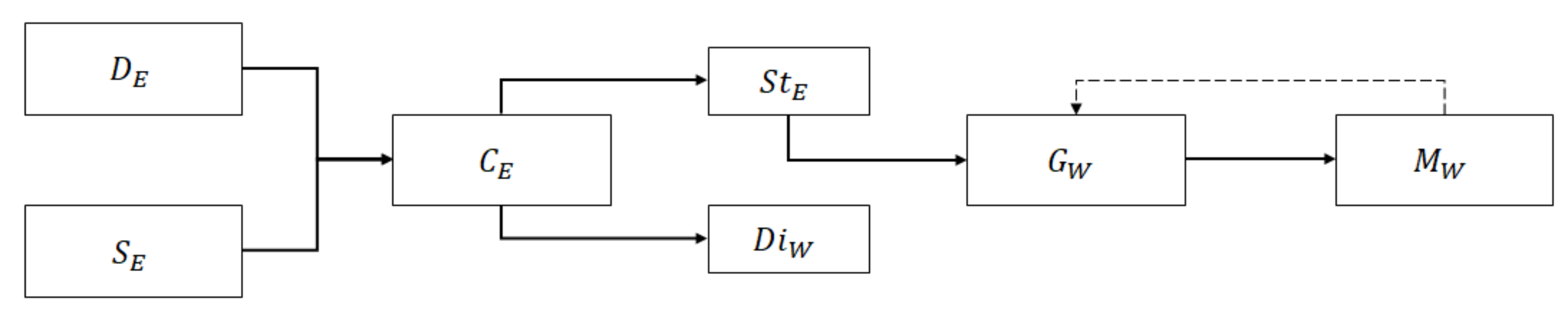
Figure 1 shows an aggregated representation of the flows and stocks structure of the EEE generation process and WEEE management system. For reference, Appendix A.1 presents all nomenclature of the SD model.

In the WEEE management system, the market behavior depends on the flow of equipment and the interaction of supply ($S_E$) and demand ($D_E$) of EEE (units). The circulation of EEE in the market ($C_E$) represents the equipment in use. When the equipment leaves circulation, it enters a transitional storage level ($S{t}_E$) or a final stage for disposition, corresponding to the disposal process ($D{i}_W$). Meanwhile, the output of the storage level depends on the rate of user waste, and this increases the level of WEEE units generated ($G_W$). Finally, the acquisition of WEEE allows for the transition from $G_W$ to the WEEE management level ($M_W$). Once WEEE enters the management level, its processing is performed following the different stages of the RL process described in Section 2.1. It is at this level where the optimization model defines key operation parameters periodically.

Equation (1) corresponds to the demand of EEE, namely, the number of people who purchase the equipment (Equation (2)). The flow $pch\left(t\right)$ is equivalent to the amount of EEE sold per person per week.

$$\begin{array}{}\hfill \mathrm{(1)}& \hfill D_E\left(t\right)& =& {\int }_{t_0}^t\left[pch\left(t\right)\right]d\left(t\right)+D_E\left(t_0\right)\hfill \hfill \mathrm{(2)}& \hfill pch\left(t\right)& =& \frac{sl\left(t\right)}{pper}\hfill \end{array}$$

The marketing of new and second-hand equipment ($mkn\left(t\right)$ and $mks\left(t\right)$, respectively) increases the supply of EEE ($S_E\left(t\right)$) (Equation (3)) and decreases it by its sales ($sl\left(t\right)$). Equation (4) represents the flow of new EEE, a stock that is subject to the rate of supply growth ($rsg$). Equation (5) shows how the flow of second-hand EEE is determined by the arrival of remanufactured equipment ($rm\left(t\right)$) thanks to the recovery management of WEEE.

$$\begin{array}{}\hfill \mathrm{(3)}& \hfill S_E\left(t\right)& =& {\int }_{t_0}^t\left[mkn\left(t\right)+mks\left(t\right)-sl\left(t\right)\right]d\left(t\right)+S_E\left(t_0\right)\hfill \hfill \mathrm{(4)}& \hfill mkn\left(t\right)& =& S_E\left(t\right)\ast rsg\hfill \hfill \mathrm{(5)}& \hfill mks\left(t\right)& =& rm\left(t\right)\hfill \end{array}$$

The flow $sl\left(t\right)$ represents the amount of equipment available to be sold ($eqa\left(t\right)$) (Equation (6)), whose value is the minimum quantity between the supply ($S_E\left(t\right)$) and the equipment demanded by new customers (Equation (7)). Equations (8) and (9) explain how the new demand of EEE ($nd\left(t\right)$) depends on the number of customers ($ctm\left(t\right)$) and their growth rate ($rcg$). The average amount of EEE per person ($pper$) multiplies the resulting value to express it in units.

$$\begin{array}{}\hfill \mathrm{(6)}& \hfill sl\left(t\right)& =& eqa\left(t\right)\hfill \hfill \mathrm{(7)}& \hfill eqa\left(t\right)& =& MIN(S_E\left(t\right);nd\left(t\right))\hfill \hfill \mathrm{(8)}& \hfill nd\left(t\right)& =& ctm\left(t\right)\ast pper\hfill \hfill \mathrm{(9)}& \hfill ctm\left(t\right)& =& D_E\left(t\right)\ast rcg\hfill \end{array}$$

The circulation of EEE ($C_E\left(t\right)$) (Equation (10)) increases due to sales of new equipment and decreases by the following two flows: first, the flow of disposal ($di\left(t\right)$) that depends on a disposal rate ($rd$) (Equation (11)), and second, the disposition flow of WEEE ($dw\left(t\right)$), which is subject to the previous level of storage (Equation (12)).

$$\begin{array}{}\hfill \mathrm{(10)}& \hfill C_E\left(t\right)& =& {\int }_{t_0}^t\left[sl\left(t\right)-di\left(t\right)-dw\left(t\right)\right]d\left(t\right)+C_E\left(t_0\right)\hfill \hfill \mathrm{(11)}& \hfill di\left(t\right)& =& C_E\left(t\right)\ast rd\hfill \hfill \mathrm{(12)}& \hfill dw\left(t\right)& =& MIN(C_E\left(t\right);out\left(t\right))\hfill \end{array}$$

The storage level in Equation (13) ($S{t}_E\left(t\right)$) increases by the amount of equipment replaced ($rpl\left(t\right)$, as defined in Equation (14), and decreases by the output of the accumulated EEE ($out\left(t\right)$, as defined in Equation (18). The replacement of equipment depends on two variables: the frequency of equipment replacement ($tm$) and the rate of unit replacement according to customer behavior ($rr\left(t\right)$) (Equation (14)). Equation (15) indicates that the replacement rate varies due to the purchase price ($epp$). This effect is represented by the GRAPH function (Equation (16)) that explains the average purchase price fluctuations ($pp\left(t\right)$) with respect to the initial average price of new EEE ($pne$) (Equation (17)) at the beginning of the simulation.

$$\begin{array}{}\hfill \mathrm{(13)}& \hfill S{t}_E\left(t\right)& =& {\int }_{t_0}^t\left[rpl\left(t\right)-out\left(t\right)\right]d\left(t\right)+S{t}_E\left(t_0\right)\hfill \hfill \mathrm{(14)}& \hfill rpl\left(t\right)& =& \frac{C_E\left(t\right)}{tm}\ast rr\left(t\right)\hfill \hfill \mathrm{(15)}& \hfill rr\left(t\right)& =& vrr\ast epp\left(t\right)\hfill \hfill \mathrm{(16)}& \hfill epp\left(t\right)& =& GRAPH\left[fp\left(t\right);t_0;\Delta t;(e{r}_1;e{r}_2;\dots e{r}_6)\right]\hfill \hfill \mathrm{(17)}& \hfill fp\left(t\right)& =& \frac{pp\left(t\right)}{pne}\hfill \end{array}$$

The EEE output of the storage level ($out\left(t\right)$) depends on the potential disposal rate (Equation (18)). This rate varies according to the effect of the economic incentive (Equation (19)). This is modeled using a GRAPH function (Equation (20)). Equation (21) describes the main argument of Equation (20) in terms of the ratio of the repurchase price ($pr$) (fixed periodically by the optimization model (25)–(57)) and the average purchase price ($pp\left(t\right)$).

$$\begin{array}{}\hfill \mathrm{(18)}& \hfill out\left(t\right)& =& S{t}_E\left(t\right)\ast rdi\left(t\right)\hfill \hfill \mathrm{(19)}& \hfill rdi\left(t\right)& =& vrdi\ast ei\left(t\right)\hfill \hfill \mathrm{(20)}& \hfill ei\left(t\right)& =& GRAPH\left[fi\left(t\right);t_0;\Delta t;(e{i}_1;e{i}_2;\dots e{i}_6)\right]\hfill \hfill \mathrm{(21)}& \hfill fi\left(t\right)& =& \frac{pr}{pp\left(t\right)}\hfill \end{array}$$

Equation (22) corresponds to the generation of WEEE ($G_W\left(t\right)$), which increases by the WEEE disposition flow ($dw\left(t\right)$) and decreases by the acquisition flow ($aq\left(t\right)$), and this is the first stage of WEEE management. The acquisition decision depends on the acquisition rate ($ra$) (Equation (23)) as an input from the optimization model.

$$\begin{array}{}\hfill \mathrm{(22)}& \hfill G_W\left(t\right)& =& {\int }_{t_0}^t\left[dw\left(t\right)-aq\left(t\right)\right]d\left(t\right)+G_W\left(t_0\right)\hfill \hfill \mathrm{(23)}& \hfill aq\left(t\right)& =& G_W\left(t\right)\ast ra\hfill \end{array}$$

Finally, Equation (24) represents WEEE stock, which increases by the acquisition of WEEE ($aq\left(t\right)$) and decreases thanks to each stage of the RL process denoted by $ciepd\left(t\right)$.

$$\begin{array}{ccc}\hfill M_W\left(t\right)& =& {\int }_{t_0}^t\left[aq\left(t\right)-ciepd\left(t\right)\right]d\left(t\right)+M_W\left(t_0\right)\hfill \end{array}$$

(24)

At this point, the optimization model determines all the decisions inside the WEEE management systems (repurchase price, acquired WEEE, export, processing and disposition flows and processing capacities). Figure 2 shows the detailed RL process performed at the $M_W$ level.

2.3. Optimization Model

The optimization model used for the iterative refinement of the SD model is a mixed-integer nonlinear program (MINLP). The decision variables (represented in grey in Figure 2) of the MINLP cover the different stages of the RL process. Meanwhile, the WEEE generation process is represented according to the structure of the SD model as depicted in Figure 1.

In the acquisition stage, the model makes three main decisions. The first one determines the repurchase price ($pr$). The second one is the amount of WEEE generated (q), which depends on the repurchase price as stated in Equation (16). The third decision is the amount of WEEE that enters the management system (x), which determines the acquisition rate ($ra$) in the SD model. Following [51], we use a piecewise linear approximation to model the WEEE generation process (i.e., to connect different repurchase price values (P) with their corresponding WEEE generation quantities (Q) in a nonlinear fashion).

Table 1. Example of the piecewise linear approximation for the WEEE generation process.

Point	$\mathit{pr}$	q	Weight $\left({\mathit{\lambda }}_{\mathit{l}}\right)$	Intervals $\left(\mathit{l}\right)$	$\left({\mathit{b}}_{\mathit{l}}\right)$
0	0	466	${\lambda }_1$	1	$b_1$
1	50	530	${\lambda }_2$	1 and 2	$b_1,b_2$
2	100	597	${\lambda }_3$	2 and 3	$b_2,b_3$
3	150	641	${\lambda }_4$	3 and 4	$b_3,b_4$
4	200	670	${\lambda }_5$	4 and 5	$b_4,b_5$
5	250	701	${\lambda }_6$	5	$b_5$

presents an example of different P values and their effect on Q. In this piecewise linear approximation, we use binary variables ($b_l$) to select a single segment of it. ${\lambda }_l$ corresponds to the weights of the extreme points of each segment in the convex combination that defines the linear interpolation used to determine the values $pr$ and q. This piecewise modeling option gives the flexibility to represent different customer behaviors that will be explored in the scenarios analyzed with the model.

Once WEEE enters the system and becomes part of the collection stage flow (x), the first decision of the RL process is to split it into two variables: WEEE sent to the inspection and sorting process ($v_f$) and WEEE exported to be treated in another country ($v_{ex}$). After inspection and sorting, the WEEE splits again into the different processing options ($k\in TR=\{elimination/deactivation,recycling,disassembly,renovation\}$) represented with variables ($y_k,k\in TR$). In this stage, we assume a lexicographic order of the different processing options. This means that the decision making process has to assign the processing options in the aforementioned order based on increasing quality. That is, lower-quality WEEE cannot be processed with an upper-quality process. For instance, WEEE suitable for cannibalization (through the disassembly process) can also be treated for recycling or elimination. On the other hand, WEEE suitable for recycling can be treated in its own process or alternatively through elimination/deactivation. Finally, after the processing option or the export phase, the resulting (valorized) materials go to the corresponding alternative markets ($w_m$) for disposition according to set m$\in C=\{export,disposal,recycledmaterials,component,second-handproducts\}$.

Additionally, the MINLP model also decides on the technologies used for the different RL processes. This decision determines for each stage of the process the available capacity, the fixed costs and the avoided environmental burden [52,53]. To model these technology-choice decisions, we use binary variables for each stage of the RL process (with $z{r}_i$ for collection, $z{f}_i$ for inspection and sorting, $ze{x}_i$ for exports and $z{p}_i^k$ for the k-th treatment alternative). Here, index i indicates the available options for each RL process. For ease of reference, Appendix A.2 presents the sets, parameters and decision variables of the MINLP model.

2.3.1. Objective Function

The main goal of the optimization model is to maximize the total profit (Equation (25)). This equation comprises four main components. The first one is the income obtained by the sales of the valorized waste ($w_m$) in each market at price $I_m$. The second one is a quadratic term that represent the cost of the repurchase of WEEE. The third component represents the variable costs of the RL process that depend on the quantities that are either exported at unitary cost $Cex$ or processed through the different treatment options at unitary cost $C{p}_k$. Finally, the last component sums up the fixed costs of the different processes determined by the technological choices (z variables) and their corresponding cost ($G{r}_i,G{f}_i,Ge{x}_i,G{t}_i^k$).

$$\begin{array}{cc}\hfill maxprofit& =\left(\sum _{m\in C}{I}_m\ast w_m\right)\hfill \\ & -(pr\ast x)\hfill \\ & -(Cex\ast v_{ex})-\left(\sum _{k\in TR}C{p}_k\ast y_k\right)\hfill \\ \hfill & -\left(\sum _{i\in T{E}_r}G{r}_i\ast z{r}_i\right)-\left(\sum _{i\in T{E}_f}G{f}_i\ast z{f}_i\right)\hfill \\ \hfill & -\left(\sum _{i\in T{E}_{ex}}Ge{x}_i\ast ze{x}_i\right)-\left(\sum _{i\in T{E}_k}\sum _{k\in TR}G{p}_i^k\ast z{p}_i^k\right)\hfill \end{array}$$

(25)

2.3.2. Constraints

The optimization model considers the following constraints to describe the WEEE generation and acquisition process: the flows inside the RL process and the capacity of the WEEE management system.

WEEE generation process. The piecewise linear approximation that relates the repurchase price and the generation of WEEE variables is given in Equations (26)–(32). The structure of these equations follows the approach described by [51]. Equation (26) ensures the choice of a single interval in the approximation. Equation (27) indicates that the point obtained is a convex combination of the extreme points of the interval. Equations (28)–(30) show the relations between the values of the variables ${\lambda }_l$ and $b_l$ using a type-2 special ordered set (SOS2) [51]. This is to calculate the convex combination where only two consecutive extreme points (in the same interval) are activated.

Finally, Equations (31) and (32) establish the values of the repurchase price and WEEE generation, respectively, using the linear combination of the extreme points of the selected interval.

$$\begin{array}{}\hfill \mathrm{(26)}& \hfill \sum _{l\in PL}{b}_l& =& 1\hfill \hfill \mathrm{(27)}& \hfill \sum _{l\in PL}{\lambda }_l& =& 1\hfill \hfill \mathrm{(28)}& \hfill {\lambda }_0& \le & b_1\hfill \hfill \mathrm{(29)}& \hfill {\lambda }_l& \le & b_{l-1}+b_l,forl=2\dots \left|PL\right|-1\hfill \hfill \mathrm{(30)}& \hfill {\lambda }_{\left|PL\right|}& \le & b_{\left|PL\right|}\hfill \hfill \mathrm{(31)}& \hfill pr& =& \sum _{l\in PL}{\lambda }_l\ast P_l\hfill \hfill \mathrm{(32)}& \hfill q& =& \sum _{l\in PL}{\lambda }_l\ast Q_l\hfill \end{array}$$

Acquisition process. Two conditions must be met at this point. The amount of WEEE acquired cannot exceed the amount of WEEE generated (Equation (33)). Additionally, a minimum acquisition amount is considered in Equation (34). In this equation, $Mr$ represents a minimum percentage of the WEEE generated to ensure an inflow into the WEEE management system.

$$\begin{array}{}\hfill \mathrm{(33)}& \hfill x& \le & q\hfill \hfill \mathrm{(34)}& \hfill x& \ge & Mr\ast q\hfill \end{array}$$

Balance constraints. This set of constraints ensures that the flow of elements is continuous through the RL process. Equation (35) indicates the collection flow splitting into inspection/sorting and export processes. Likewise, Equation (36) indicates that after inspection, the flow of WEEE is split into the different processing options.

$$\begin{array}{}\hfill \mathrm{(35)}& \hfill x& =& v_f+v_{ex}\hfill \hfill \mathrm{(36)}& \hfill v_f& =& \sum _{k\in TR}{y}_k\hfill \end{array}$$

WEEE state constraints. These constraints define the appropriate processing alternatives according to the initial status of the WEEE determined after inspection and sorting, and consequently, its ideal market alternative. To model the WEEE entering status, we use parameters $S{p}_k$ to express the percentage of WEEE entering the system that is suitable for the treatment option k ($k\in TR$, i.e., the options of the RL processing stage). Equations (37) and (38) indicate the amount of WEEE that can enter each processing option according to their initial status. Particularly, Equation (39) ensures the amount of WEEE that has to be eliminated because no other option is available given its initial status (that is, the percentage of WEEE with status $S{p}_{disposal}$). Finally, Equation (40) determines the amount of materials available in each market ($m\in C$) after treated with the different processes ($k\in TR$). In this last equation, we resort to parameter $S{c}_{k,m}$ to represent the percentage of WEEE suitable for market m after process k. In a special case, the amount of WEEE that is directly exported and does not enter the internal RL process is given in Equation (41).

$$\begin{array}{}\hfill \mathrm{(37)}& \hfill y_k& \le & v_f\sum _{k^{\prime }\in k:k^{\prime }\le k}S{p}_k;\forall k\in TR\hfill \hfill \mathrm{(38)}& \hfill \sum _{k^{\prime }\in TR:k^{\prime }\le k}{y}_k& \le & v_f\sum _{k^{\prime }\in TR:k^{\prime }\le k}S{p}_k;\forall k\in TR\hfill \hfill \mathrm{(39)}& \hfill y_k& \ge & v_f\ast S{p}_k;k=disposal\hfill \hfill \mathrm{(40)}& \hfill w_m& =& \sum _{k\in TR}{y}_k\ast S{c}_{k,m};\forall m\in C\backslash \left\{export\right\}\hfill \hfill \mathrm{(41)}& \hfill w_{ex}& =& v_{ex}\hfill \end{array}$$

Capacity constraints. Equations (42)–(49) define (respectively) the capacities of the different stages of the RL process according to the selected technologies. In these constraints, available capacities are represented by the following parameters: $H{r}_i$ for collection, $H{f}_i$ for inspection and sorting, $He{x}_i$ for export and $H{p}_i^k$ for the treatments of the processing stage.

$$\begin{array}{}\hfill \mathrm{(42)}& \hfill \sum _{i\in T{E}_r}z{r}_i& =& 1\hfill \hfill \mathrm{(43)}& \hfill x& \le & \sum _{i\in T{E}_r}H{r}_i\ast z{r}_i\hfill \hfill \mathrm{(44)}& \hfill \sum _{i\in T{E}_f}z{f}_i& =& 1\hfill \hfill \mathrm{(45)}& \hfill v_f& \le & \sum _{i\in T{E}_f}H{f}_i\ast z{f}_i\hfill \hfill \mathrm{(46)}& \hfill \sum _{i\in T{E}_{ex}}ze{x}_i& =& 1\hfill \hfill \mathrm{(47)}& \hfill v_{ex}& \le & \sum _{i\in T{E}_{ex}}He{x}_i\ast ze{x}_i\hfill \hfill \mathrm{(48)}& \hfill \sum _{i\in T{E}_k}z{p}_i^k& =& 1;\forall k\in TR\hfill \hfill \mathrm{(49)}& \hfill y_k& \le & \sum _{i\in T{E}_t}H{p}_i^k\ast z{p}_i^k;\forall k\in TR\hfill \end{array}$$

Market demand. Finally, at the disposition stage, the amount of valorized material that goes to each market is limited by its demand (Equation (50)).

$$\begin{array}{ccc}\hfill w_m& \le & D_m;\forall m\in C\hfill \end{array}$$

(50)

Variable domain constraints. Constraints (51) to (57) define the decision variables and their domains.

$$\begin{array}{}\hfill \mathrm{(51)}& \hfill pr,q,x,v_f,v_{ex}& \ge & 0\hfill \hfill \mathrm{(52)}& \hfill y_k& \ge & 0,k\in TR\hfill \hfill \mathrm{(53)}& \hfill w_m& \ge & 0,m\in C\hfill \hfill \mathrm{(54)}& \hfill {\lambda }_l& \ge & 0,l\in PL\hfill \hfill \mathrm{(55)}& \hfill b_l& \in & \{0,1\},l\in PL\hfill \hfill \mathrm{(56)}& \hfill z{r}_i,z{f}_i,ze{x}_i,& \in & \{0,1\},i=1,\dots ,O{p}_s,s\in RL\backslash \left\{TR\right\}\hfill \hfill \mathrm{(57)}& \hfill z{p}_i^k,& \in & \{0,1\},i=1,\dots ,O{p}_k,k\in TR\hfill \end{array}$$

2.3.3. Environmental Indicator (Alternative Objective Function)

To measure the environmental effect of the system, we used the Avoided Environmental Burden (AEB) indicator. Introduced by [53], the AEB is an alternative multidimensional metric to assess WEEE management systems that focuses its attention on the recovery of raw materials and the environmental benefits of recycling them. The dimensions of the AEB include cumulative energy demand, global warming potential, human toxicity potential, acidification and nutrification, among others. In our computational experiments, we explore the effect of the WEEE management system on profits if the AEB indicator is used as alternative objective function. To measure the AEB, we use the primary material extraction avoidance that comes from the different RL processes as presented by [53]. Equation (58) presents the AEB metric used in the proposed approach. Note that the AEB expression has a non-linear structure since it includes in each one of its terms the multiplication of the volume disposed in each market ($w_{ex}$ and $w_m,m\in C$), its environmental burden ($B_{ex},B_m,m\in C$), the AEB obtained ($Ae{x}_i$ and $A{p}_i^k,k\in TR$) by the (technological) option chosen for the export stage and each treatment process ($ze{x}_i,z{p}_i^k,k\in TR$).

$$AEB=B_{ex}\ast w_{ex}\left(\sum _{i\in T{E}_{ex}}Ae{x}_i\ast ze{x}_i\right)+\sum _{m\in C}{B}_m\ast w_m\left(\sum _{i\in T{E}_k}\sum _{k\in RL}A{p}_i^k\ast z{p}_i^k\right)$$

(58)

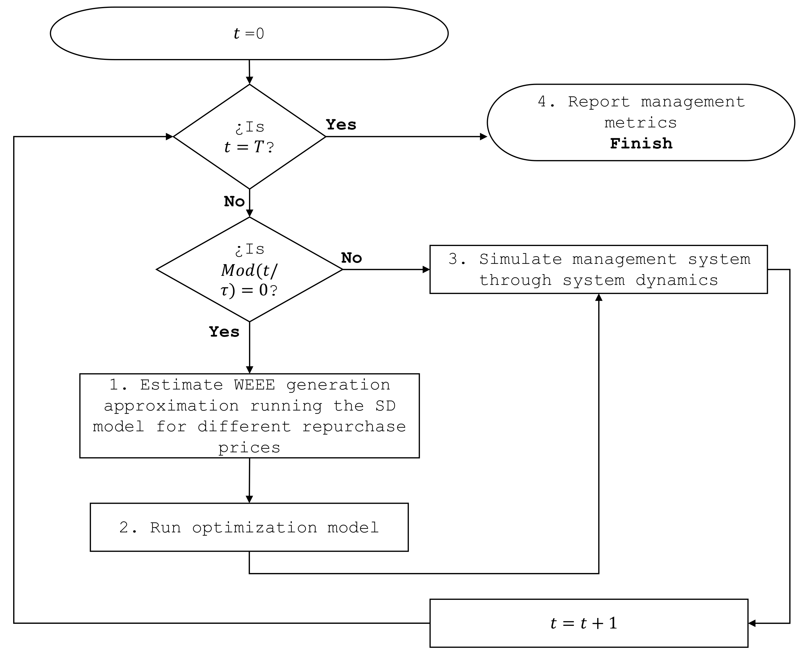
2.4. OBS Implementation

Figure 3 summarizes the implementation of the OBS approach following the procedure depicted on it. The simulation step is equivalent to one week (t), and the simulation ends when it reaches the time horizon (T). In general, the steps described in Figure 3 are:

• Estimate WEEE generation. Initially, at the beginning of each cycle, SD is used to estimate the effect of several repurchase prices and its corresponding generation of WEEE according to the dynamics of the market described in Section 2.2. This procedure updates the values used in the piecewise linear approximation of the optimization model (Equations (26)–(32)) and in the GRAPH function for the WEEE generation process of the SD model (Equation (20)). In this step, we test iteratively increasing values of $pr$ (beginning at a given value $p{p}_0$ equal to 0) and store the corresponding values of q.
• Run the optimization model. Using the previous estimates, in this step, the optimization model (of Section 2.3) chooses the optimal point for the repurchase price ($pr$) and its corresponding generation of WEEE (q). Simultaneously, the optimization model also specifies the flow entering the RL process x and the flows inside it (variables $v,y$ and w), as well as the capacities of the different stages (variables z).
• Simulate the WEEE management system. At this step, the SD model (Section 2.2) considers the output of the optimization model and uses the Euler integration method to model the interaction between flows and levels of the WEEE management system ($D_E,S_E,C_E,S{t}_E,D{i}_W,G_W$). At the WEEE generation level ($G_W$), the simulation uses again the estimates of the piecewise linear approximation ($Pl,Q_l,l\in PL$) and represents the WEEE management level ($M_W$) with the RL processes inside it. The SD model runs under these conditions for a period of $\tau$ weeks. Once the reoptimization period ($\tau$) is reached, the procedure runs step 1 for a new WEEE generation estimate and step 2 for a reoptimization of the RL process.
• Report performance metrics. Once the simulation horizon (T) is reached, four different performance metrics of the system are reported: (i) the total profit, (ii) the total AEB, (iii) the total number of units of WEEE processed by the WEEE management system and (iv) the average repurchase price.

The SD model was implemented in Excel for its connection with the optimization model. The optimization model was developed on the OpenSolver platform [54] using Couenne [55] as the non-linear optimizer under the NEOS optimization service [56]. The OBS approach was implemented through Visual Basic for Applications to automate the information transfer and to provide the end-user with a visual interface where it is possible to select the conditions of the desired experimental runs [57].

3. Results and Discussion

This section illustrates the benefits of the proposed OBS approach as a tool for policy optimization to improve the design of a WEEE management system. First, we validate the effect of embedding an optimization model inside the system dynamics model. Then, after validation, we explore different scenarios of a WEEE management system for mobile phones in Colombia with the help of the proposed approach. This case study illustrates how the OBS approach selects the conditions under which the WEEE management system can achieve optimal performance.

3.1. Case Study: Colombian Mobile Phones

As a case study, we chose mobile phones (MPs) in the Colombian context for several reasons. First, MPs are the current focus of a post-consumption policy in progress in the Colombian legislation [58]. Second, Ref. [4] addressed WEEE from MPs in the Colombian context using SD. However, in their model, they do not explicitly include the reverse logistics system and its design. They rather focus on the WEEE generation process and how different variables affect it. Particularly, they show that the high replacement dynamism of MPs can be one of the main factors determining WEEE generation of MPs in Colombia. Therefore, we analyze this variable in one of the proposed scenarios. Likewise, they propose the study of economic incentives to end-users (e.g., buy-back programs and discounts offered to customers that bring their old MPs). We analyze such mechanisms through computational experiments. The input data were collected between 2017 and 2018, and the relevant time horizon for simulation is 2018–2037.

Table 2. Description and input data for the illustrative example.

Variables	Description/Input Data	Source
Marketing of EEE	Weekly growth rate of EEE supply: 0.070%	[32,59,60]
Purchase of EEE	Weekly growth rate of EEE demand: 0.064%	[32,61]
Replacement of EEE	Potential weekly replacement rate of EEE: 0.077% Frequency of purchase of a new EEE: every 74 weeks	[62,63]
Repurchase price	Monetary incentive and willingness to dispose their EEE	[35]
Management of WEEE	RL process costs, revenues and environmental impact for each stage and market	[12,52,64,65,66]

presents a synthesis of the main input data for the model.

3.2. Optimization-Based Optimization Benefits

After the customary SD validation of the model structure, dimensional consistency and parameter assessment [67], we analyze the relevance of the OBS integration. In this regard, the usefulness of the proposed approach comes from the comparison of the outcomes in performance of two scenarios. The base case scenario only applies for Simulation. The management decisions (entering WEEE into the system, flows of elements between RL stages and technology option selection) are defined and fixed at the beginning of the simulation start time. The second scenario follows the proposed OBS approach (Simulation+Profit Maximization), and contrary to the first scenario, management decisions are updated annually according to the values provided by the optimization. Moreover, to see the effect of the economic incentive adjustment done by the optimization model (variable $pr$), in both scenarios the initial repurchase price is set to zero, but the OBS scenario is allowed to (optimally) update it.

Figure 4 shows the evolution of the weekly generation of WEEE for the SD simulation-only scenario and the proposed OBS approach scenario. This result shows how under an OBS approach, the system increases its capacity of disposing WMP. The saw-like behavior presented in Figure 4 corresponds to the periods where the parameters are updated and the operation conditions are reconfigured accordingly.

Figure 5 compares all the performance metrics of waste mobile phones (WMPs) under the base case scenario and the OBS approach under a profit maximization objective (Simulation vs. Simulation + Profit Optimization). The figure shows how the results under the OBS approach achieve better outcomes in all dimensions. The corresponding scenario has a volume of WEEE that is 36% superior, causing a positive increase in profits of 33% and an increase of 65% in AEB.

According to the above results, the OBS approach provides better performance in all the metrics when compared to the SD simulation-only scenario where the system is not allowed to react to the changing environment through the update of optimal policies. This result illustrates that making periodical optimization decisions during the simulation benefits the outcomes of both the economy and the environment.

Environmental vs. Economic Optimization Comparison

As an additional comparison, a third scenario is proposed to evaluate the operation of the system under a different objective to be maximized. While the initial OBS scenario operates the system by maximizing the economic benefits (defined in Figure 5 as profit optimization), the third scenario seeks the operation of the system considering the environmental impact as the main goal. The Simulation + Environmental optimization scenario maximizes the environmental benefits through the AEB indicator (Figure 5). The comparison between these conflicting objectives characterizes a common dilemma among environmentally conscious companies or companies considering the adoption of these values. Additionally, the purpose of this comparison is to test the economic feasibility of this kind of industry when just prioritizing an environmental goal. Moreover, it is necessary to analyze in this kind of industry, which already incorporates circular economy principles, up to what point the maximization of economic benefits yields environmental outcomes.

The results presented in Figure 5 compare the change of one policy with respect to the other. The OBS approach shows how, in order to maximize an environmental objective, the repurchase price must be increased as an incentive to drive more WEEE generation. This outcome is a result of a greater availability of waste that increases the recovery rate of reusable materials, which ultimately creates a positive effect on the environmental performance AEB. Nevertheless, such effort to collect more waste through an increase in the repurchase price decreases profits because the repurchase price to buy waste has to increase to induce disposal. Conversely, when the model maximizes economic benefits, it decreases the purchase price by almost 50% and reduces the generation of WEEE as well as the AEB performance. As a consequence, these decisions increase profits by 32%.

3.3. Scenario Analysis

Once the capacity of the OBS approach to outperform the SD simulation-only outcomes is introduced, the analysis focuses on testing different scenarios to explore the versatility of the OBS approach to determine the optimal policies for the operation of a WEEE management system. To do so, we evaluate four scenarios, among many possible, which were selected because they incorporate the key elements of the WEEE management system outlined in the Colombian WMP’s context by [4]. Thus, the first scenario analyzes the benefits of incorporating an RL process that looks for the valorization of the WEEE generated against a policy aimed at elimination. The second scenario analyzes the effect of the processing capacity on the RL process performance. The third scenario evaluates the effect of different replacement frequency of mobile phones on the performance of the system. Finally, the fourth scenario analyzes the customer expectations towards repurchase price of WEEE. These scenarios are not just revealing insights about the structure and behavior of the WEEE management system but also validating the potential of the OBS approach to deal with the complexities of the decision-making process.

3.3.1. Treatment Alternatives Scenario

This scenario analyzes the impact of the reverse logistics process on WEEE management. The results presented in Figure 6 illustrate how the RL Valorization scenario (corresponding to the Simulation + Profit maximization results) dominates an elimination alternative in all its metrics. The Elimination scenario is obtained by increasing the amount of WMPs that go to the disposal with parameter $S{p}_{disposal}$ in Equation (39). The valorization alternative yields 93% more profits, allowing a higher repurchase price. This capability induces the generation of WEEE, and consequently, a better environmental performance measured in a 127% higher AEB. On the contrary, the elimination alternative does poorly in the generation of profits and WEEE, affecting its capabilities of increasing the repurchase price and the AEB. This comparison reveals the importance of a RL process to prevent large amounts of WEEE going to landfills or incineration facilities, offering both environmental and economic benefits. Moreover, these results reinforce the importance of WEEE valorization regulation, optimized policies and programs for developing countries such as Colombia [68].

3.3.2. Processing Capacity Impact

Once the importance of the RL process has been demonstrated, we explore the effect of the available WEEE processing capacity on the performance of the system. To analyze this variable, in a shortfall capacity scenario, we halved the values of the capacities in the different stages of the RL process, and the fixed costs were reduced accordingly. Figure 7 compares this scenario against the base-case scenario (Simulation + Profit maximization results). This scenario processes 26% less WMPs, and this, in turn, results in a reduction of 39% in the profits and 43% in the AEB of the system. This scenario shows that having an RL process is not enough; it must also have enough capacity to process the generated WEEE. If not, the environmental and economic benefits of this system are not completely achieved.

3.3.3. MPs Frequency of Replacement Effect

The replacement frequency of MPs is one of the main variables determining the generation of WEEE [4]. It is defined by the time period that elapses between the moment of the cellphone purchase and the moment in which the customer decides to replace it. The model compares the performance of the system under three different frequency rates of replacement (scenarios). All three scenarios are compared under the main objective of maximizing profits. The first frequency rate of 18 months is determined as a base-case scenario, in accordance with the literature [63]. The second scenario considers a fast frequency of replacement of 6 months, and the third scenario considers a slow frequency of 24 months. Figure 8 presents the comparative results of the three scenarios.

The results presented in Figure 8 are explained by the effect of replacement frequency on WEEE generation. When the replacement frequency is 6 months, the generation is fast, and consequently, there is no need to increase the repurchase price as an incentive to promote WMP disposal. As a result, the average repurchase price of this fast replacement scenario is 58% of the base-case repurchase price. This situation produces an increase of 54% on profits and 62% on the AEB.

In contrast, the 24-month replacement frequency scenario portrays opposite results. If the generation is low, the optimization is forced to increase the purchase price for inducing WEEE disposal. However, the decrease in profits counterbalances the increase in repurchase price, placing it at an inferior level compared to the price level reached in the base-case scenario (i.e., 80% of the base-case repurchase price). The impossibility of increasing the repurchase price decreases the system capacity to induce WEEE and reduces the profits to 47% and the AEB to 57% of the base-case values.

These results are in line with the findings of [69], highlighting the importance of an optimized RL process that is capable to adapt to short product life cycles such as those of the MP industry.

3.3.4. Customer Repurchase Price Expectations

As pointed out by [69], customer behavior is a key factor in the success of WMP management systems. Previous studies in BRIC and developing countries [70,71,72] emphasize the importance of different economic incentives to promote end-user recycling of their old MPs. Therefore, in this analysis, we consider three scenarios which present different WEEE repurchase price expectations of the users. These scenarios are modeled by changing Equations (18)–(21) of the system dynamics model and Equations (26)–(32) in the optimization model.

Figure 9 presents the results of these scenarios. The first customer is one with high expectations (High behavior), willing to sell their device if the repurchase price is close enough to the original purchase price. The second one is a user whose expectations are zero, which supposes they are willing to donate their device if they need an update (Altruistic behavior). The third type is a user who is willing to sell their device at a price inferior to 50% of the original price (Moderate behavior). All three scenarios are compared under the main objective of maximizing profits.

These results illustrate how the system reacts to different customer repurchase price expectations. The first expectation has the lowest repurchase price of the three levels because the customer is willing to donate their used phone. This result has two consequences: the first one is positive because the low repurchase price increases profits by 10%, and the second one is negative because the economic incentive is not a trigger to induce more WMP recycling. Consequently, the number of WMPs processed decreases by 7.8% and the AEB by 8.9%. This is because we are assuming that this customer is completely altruistic, and the economic incentive is not the main driver to donate their device.

On the other hand, customers influenced by repurchase prices are considered among the categories of moderate and high expectation levels. The OBS approach offers the customer with high repurchase price expectations a 33% lower repurchase price compared to the price offered to the moderate expectation customer (i.e., the base-case repurchase price). This result is counter-intuitive because it is expected that the repurchase price should be higher than the price offered to the moderate customer. However, a very high repurchase price needed to foster WEEE generation reduces the profits. As a result, profits in the moderate-expectation scenario are 30% higher than those of the high-expectation scenario, and 25% more WMPs are collected. However, the altruistic behavior has even greater profits since it does not need to incur in the repurchasing cost to trigger WEEE generation.

4. Conclusions and Perspectives

This paper presents an OBS approach that allows the design of sustainable WEEE management system policies. By integrating optimization and system dynamics in the hybrid approach described in this paper, the analysis profits from the complementary strengths of each methodology. Optimization methodologies find optimal solutions in defined and limited sets of time. The simulation describes the behavior of polices over time, which are unable to optimally self-correct. The model presented here is an example of how the OBS approach could be implemented to tackle interdependent strategic and systemic problems governed by feedback and nonlinearities such as those of WEEE management systems and the circular economy.

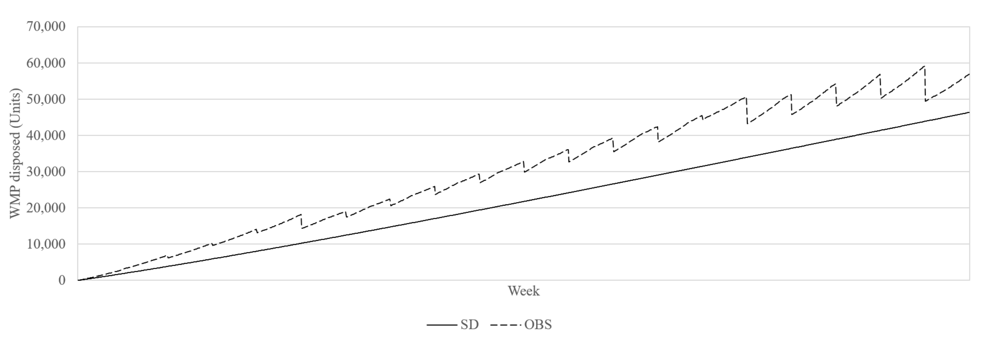
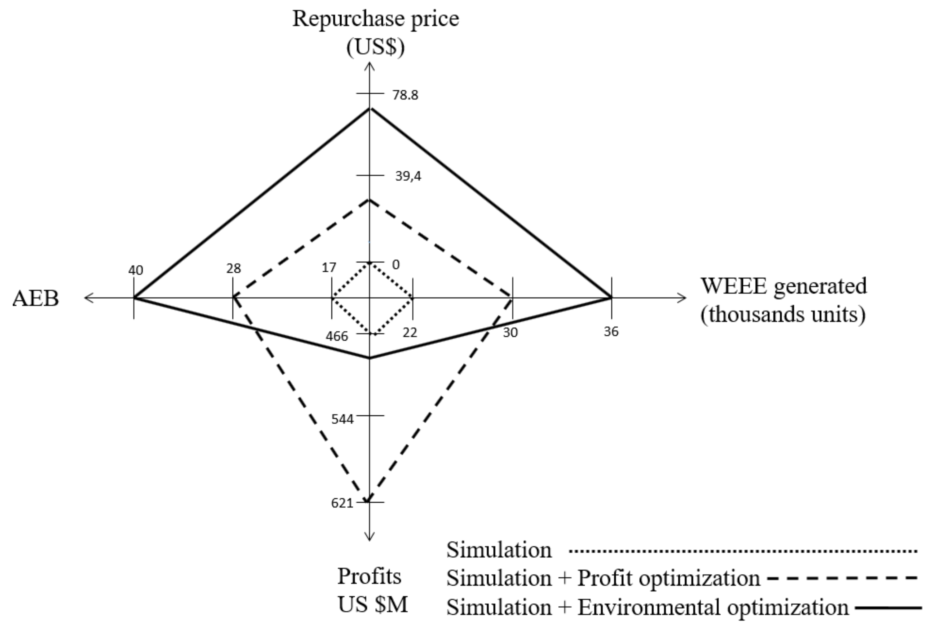
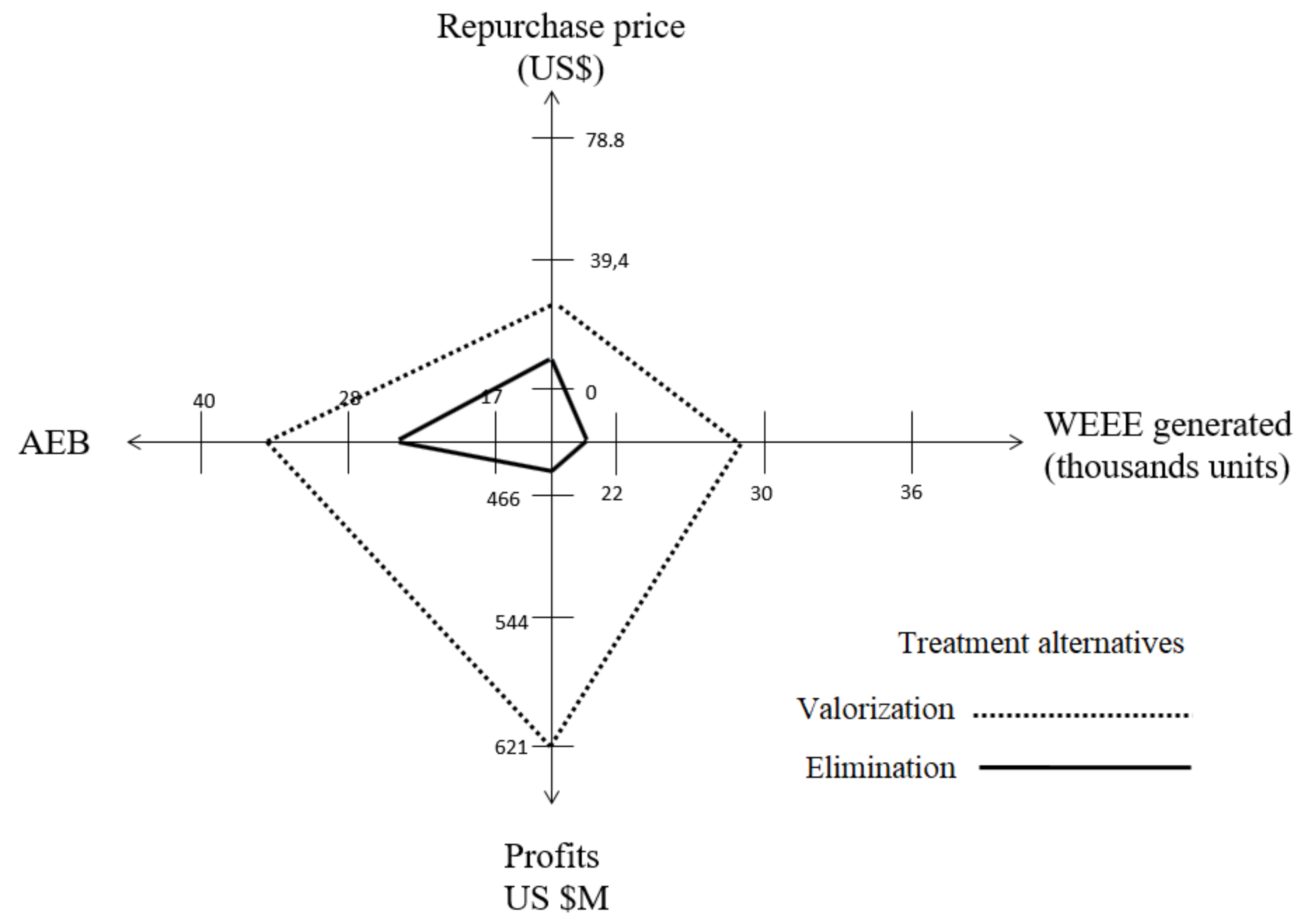
The computational results in a case study based on WEEE from Colombian mobile phones illustrates how an approach solely based on simulation (under the widely used system dynamics paradigm) is unable to capture the operative-strategic nature of the system and perform optimal parameter updates. In contrast, the OBS approach of this paper outperforms the SD approach in several dimensions. In general, it is able to obtain 33% more profits and 65% more environmental benefits mainly obtained by a 36% greater quantity of WEEE entering the system to be treated and valorized.

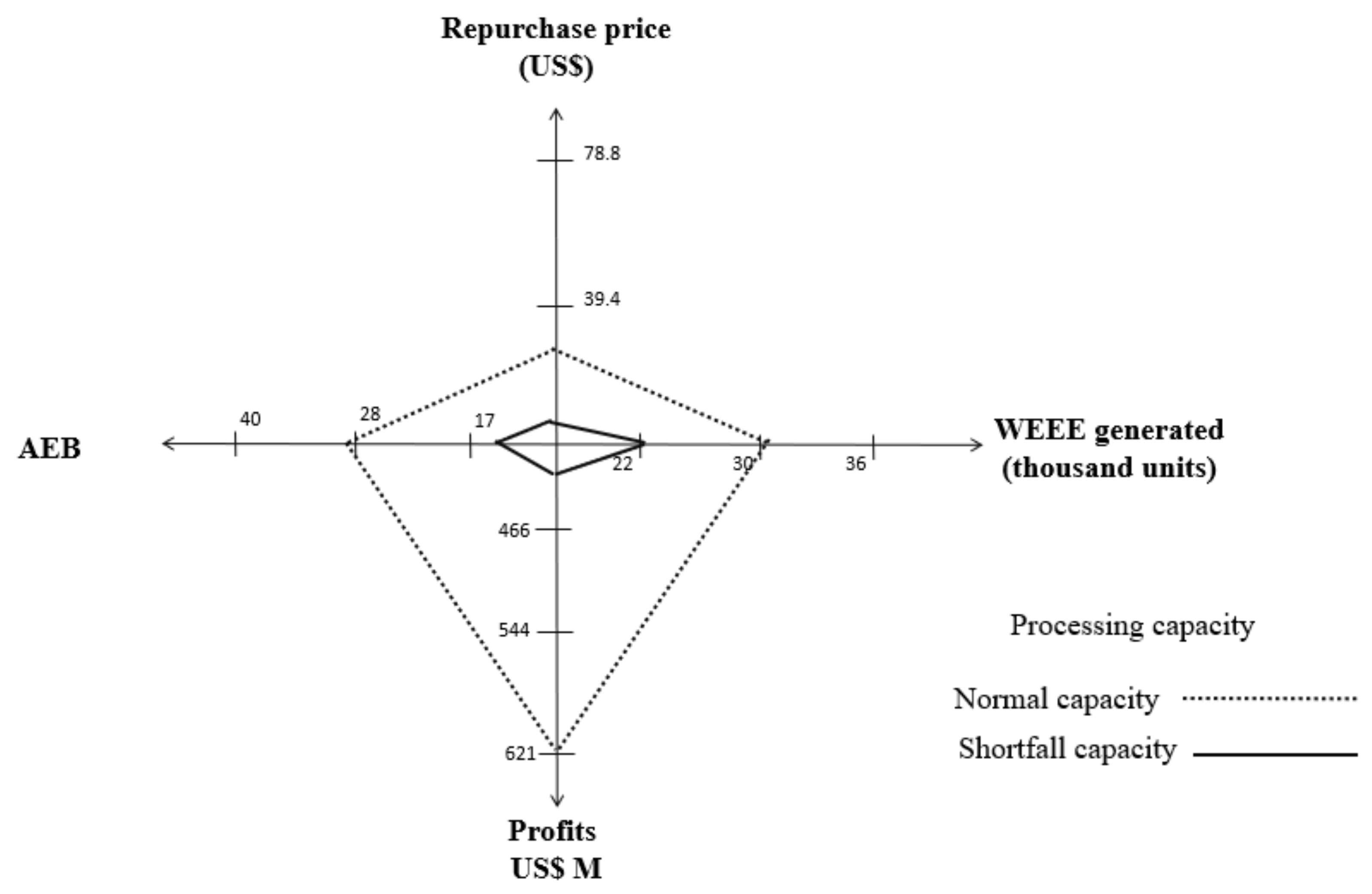
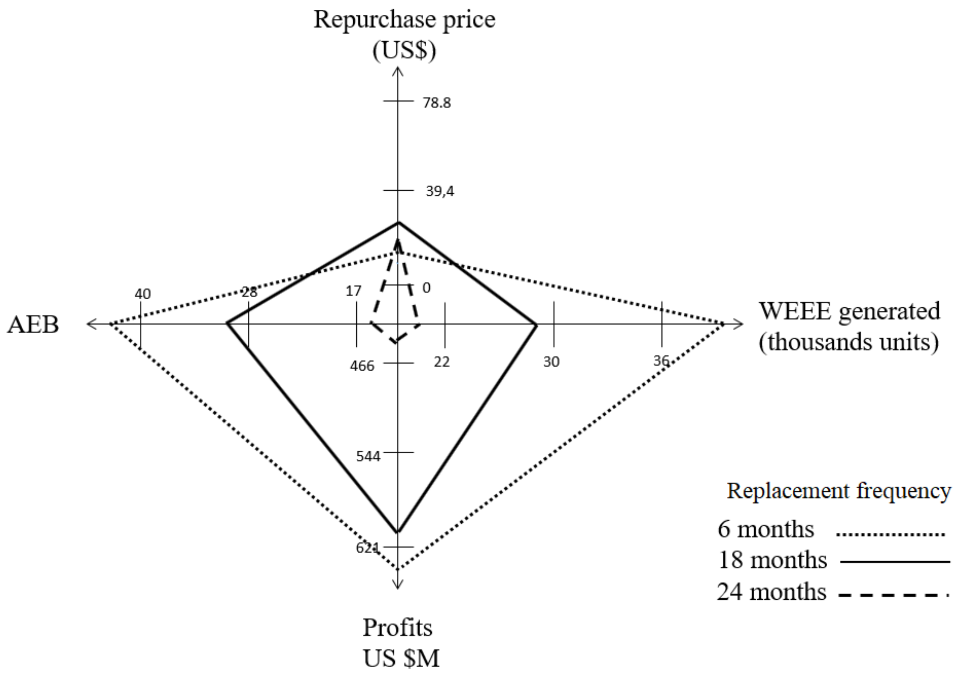
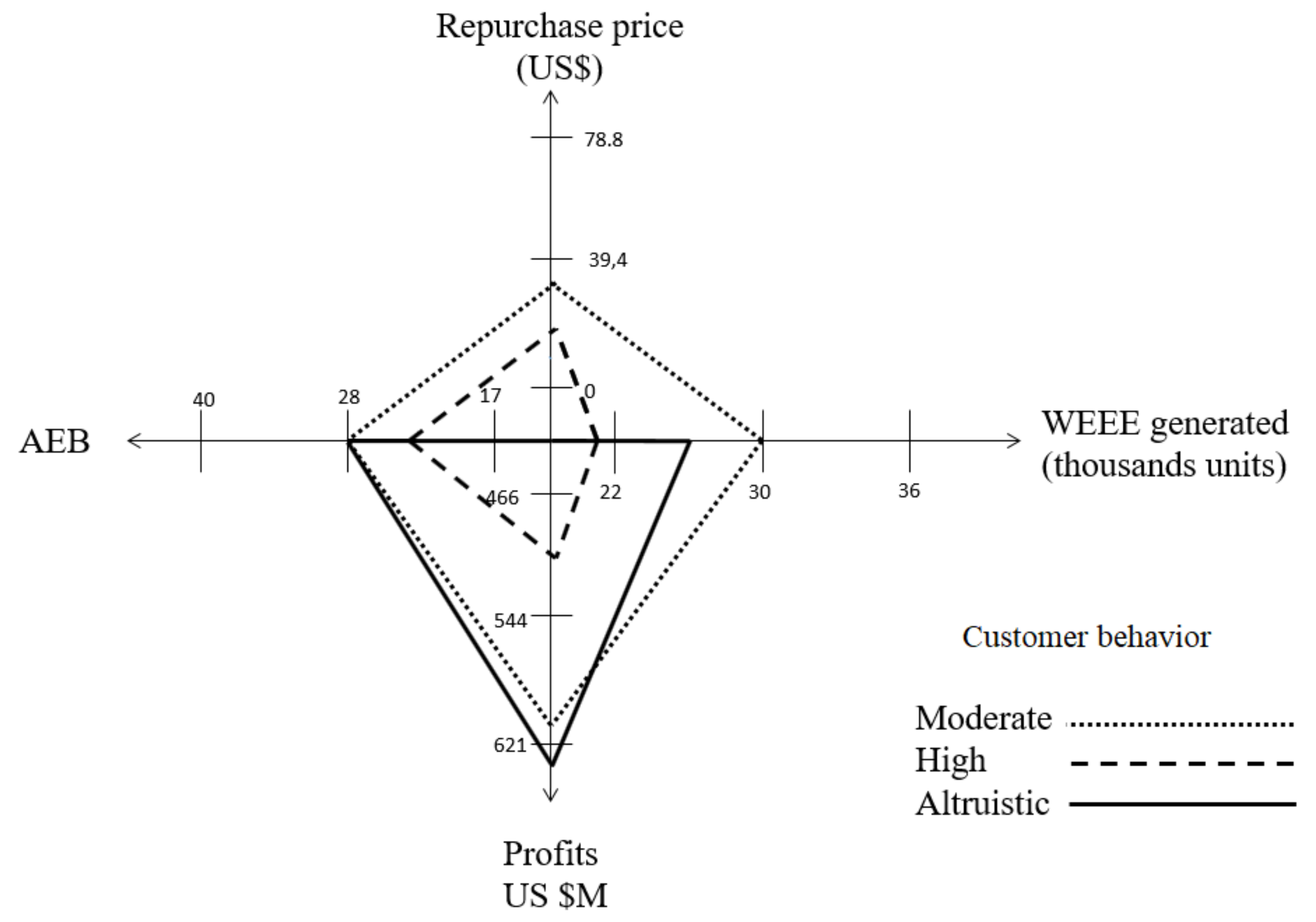
Moreover, by dynamically adjusting the repurchase price of WEEE and the structure (flows and capacities) of the reverse logistics process, the OBS is capable of positively reacting to a wide variety of scenarios with different replacement frequencies, customer expectations towards an economic incentive or different prevailing alternatives in the treatment of WEEE and processing capacities. The analysis of these scenarios allows the identification of the main drivers used in the design of optimal WEEE management system policies. The results presented here suggest that a maximization of profits can yield both economic profits and environmental savings in this kind of industry. The model suggests that the cornerstone of the WEEE management system is the replacement rate which is influenced by two main drivers: the frequency of replacement and the customer repurchase price expectations.

The OBS approach proposed in this paper can be extended in different ways. The first possible extension is considering a bi-objective model that explicitly includes the economic/environmental trade-off. This extension will need a multi-objective approach for the optimization component. Another possible extension is to include randomness into the SD model to better describe some of the system elements (e.g., WEEE generation, status and prices). Finally, the role of the informal sector (an important factor in developing economies [70,71,73]) could be added to the system dynamics model.

References

1. Cucchiella, F.; D’Adamo, I.; Lenny Koh, S.C.; Rosa, P. Recycling of WEEEs: An economic assessment of present and future e-waste streams. Renew. Sustain. Energy Rev. 2015, 51, 263–272. [Google Scholar] [CrossRef] [Green Version]
2. Mihai, F.C.; Gnoni, M.G.; Meidiana, C.; Ezeah, C.; Elia, V. Waste Electrical and Electronic Equipment (WEEE): Flows, Quantities, and Management—A Global Scenario. In Electronic Waste Management and Treatment Technology; Elsevier: Amsterdam, The Netherlands, 2019; pp. 1–34. [Google Scholar]
3. Ilankoon, I.M.S.K.; Ghorbani, Y.; Chong, M.N.; Herath, G.; Moyo, T.; Petersen, J. E-waste in the international context–A review of trade flows, regulations, hazards, waste management strategies and technologies for value recovery. Waste Manag. 2018, 82, 258–275. [Google Scholar] [CrossRef]
4. Galeano, D.A.R.; Rodríguez, S.C.B. An integrated method of environmental analysis and system dynamics for management of mobile phone waste in Colombia. J. Clean. Prod. 2021, 279, 123768. [Google Scholar] [CrossRef]
5. Ardi, R.; Leisten, R. Assessing the role of informal sector in WEEE management systems: A System Dynamics approach. Waste Manag. 2016, 57, 3–16. [Google Scholar] [CrossRef] [PubMed]
6. Kaya, M. Recovery of metals and nonmetals from electronic waste by physical and chemical recycling processes. Waste Manag. 2016, 57, 64–90. [Google Scholar] [CrossRef] [PubMed]
7. Zhang, L.; Xu, Z. A review of current progress of recycling technologies for metals from waste electrical and electronic equipment. J. Clean. Prod. 2016, 127, 19–36. [Google Scholar] [CrossRef]
8. Forti, V.; Balde, C.P.; Kuehr, R.; Bel, G. The Global E-waste Monitor 2020: Quantities, Flows and the Circular Economy Potential. United Nations University. 2020. Available online: http://ewastemonitor.info/ (accessed on 13 October 2021).
9. Zeng, X.; Duan, H.; Wang, F.; Li, J. Examining environmental management of e-waste: China’s experience and lessons. Renew. Sustain. Energy Rev. 2017, 72, 1076–1082. [Google Scholar] [CrossRef]
10. De Souza, R.G.; Clímaco, J.C.N.; Sant’Anna, A.P.; Rocha, T.B.; do Valle, R.d.A.B.; Quelhas, O.L.G. Sustainability assessment and prioritisation of e-waste management options in Brazil. Waste Manag. 2016, 57, 46–56. [Google Scholar] [CrossRef] [Green Version]
11. Salhofer, S.; Steuer, B.; Ramusch, R.; Beigl, P. WEEE management in Europe and China—A comparison. Waste Manag. 2016, 57, 27–35. [Google Scholar] [CrossRef]
12. Achillas, C.; Vlachokostas, C.; Aidonis, D.; Moussiopoulos, N.; Iakovou, E.; Banias, G. Optimising reverse logistics network to support policy-making in the case of Electrical and Electronic Equipment. Waste Manag. 2010, 30, 2592–2600. [Google Scholar] [CrossRef]
13. Achillas, C.; Vlachokostas, C.; Moussiopoulos, N.; Perkoulidis, G.; Banias, G.; Mastropavlos, M. Electronic waste management cost: A scenario-based analysis for Greece. Waste Manag. Res. 2014, 29, 963–972. [Google Scholar] [CrossRef] [PubMed]
14. Dias, P.; Machado, A.; Huda, N.; Bernardes, A.M. Waste electric and electronic equipment (WEEE) management: A study on the Brazilian recycling routes. J. Clean. Prod. 2018, 174, 7–16. [Google Scholar] [CrossRef]
15. Perkins, D.N.; Drisse, M.N.B.; Nxele, T.; Sly, P.D. E-waste: A global hazard. Ann. Glob. Health 2014, 80, 286–295. [Google Scholar] [CrossRef]
16. Temur, G.T.; Bolat, B. Evaluating efforts to build sustainable WEEE reverse logistics network design: Comparison of regulatory and non-regulatory approaches. Int. J. Sustain. Eng. 2017, 10, 358–383. [Google Scholar] [CrossRef]
17. Sepúlveda, A.; Schluep, M.; Renaud, F.G.; Streicher, M.; Kuehr, R.; Hagelüken, C.; Gerecke, A.C. A review of the environmental fate and effects of hazardous substances released from electrical and electronic equipments during recycling: Examples from China and India. Environ. Impact Assess. Rev. 2010, 30, 28–41. [Google Scholar] [CrossRef]
18. D’Adamo, I.; Ferella, F.; Gastaldi, M.; Maggiore, F.; Rosa, P.; Terzi, S. Towards sustainable recycling processes: Wasted printed circuit boards as a source of economic opportunities. Resour. Conserv. Recycl. 2019, 149, 455–467. [Google Scholar] [CrossRef]
19. Li, X.; Mu, D.; Du, J.; Cao, J.; Zhao, F. Game-based system dynamics simulation of deposit-refund scheme for electric vehicle battery recycling in China. Resour. Conserv. Recycl. 2020, 157, 104788. [Google Scholar] [CrossRef]
20. Alumur, S.A.; Nickel, S.; Saldanha-da Gama, F.; Verter, V. Multi-period reverse logistics network design. Eur. J. Oper. Res. 2012, 220, 67–78. [Google Scholar] [CrossRef]
21. Agrawal, S.; Singh, R.K.; Murtaza, Q. A literature review and perspectives in reverse logistics. Resour. Conserv. Recycl. 2015, 97, 76–92. [Google Scholar] [CrossRef]
22. Agarwal, G.; Barari, S.; Tiwari, M.K. A PSO-based optimum consumer incentive policy for WEEE incorporating reliability of components. Int. J. Prod. Res. 2012, 50, 4372–4380. [Google Scholar] [CrossRef]
23. Sterman, J.D. Business Dynamics: Systems Thinking and Modeling for a Complex World; McGraw-Hill: New York, NY, USA, 2000. [Google Scholar]
24. Topcu, A.; Benneyan, J.C.; Cullinane, T.P. A simulation-optimisation approach for reconfigurable inventory space planning in remanufacturing facilities. Int. J. Bus. Perform. Supply Chain. Model. 2013, 5, 86–114. [Google Scholar] [CrossRef]
25. Joshi, B.V.; Vipin, B.; Ramkumar, J.; Amit, R. Impact of policy instruments on lead-acid battery recycling: A system dynamics approach. Resour. Conserv. Recycl. 2021, 169, 105528. [Google Scholar] [CrossRef]
26. Matsumoto, M. Development of a simulation model for reuse businesses and case studies in Japan. J. Clean. Prod. 2010, 18, 1284–1299. [Google Scholar] [CrossRef]
27. Pandian, G.R.S.; Abdul-Kader, W. Performance evaluation of reverse logistics enterprise—An agent-based simulation approach. Int. J. Sustain. Eng. 2017, 10, 384–398. [Google Scholar] [CrossRef] [Green Version]
28. Gamberini, R.; Gebennini, E.; Manzini, R.; Ziveri, A. On the integration of planning and environmental impact assessment for a WEEE transportation network—A case study. Resour. Conserv. Recycl. 2010, 54, 937–951. [Google Scholar] [CrossRef]
29. Govindan, K.; Soleimani, H.; Kannan, D. Reverse logistics and closed-loop supply chain: A comprehensive review to explore the future. Eur. J. Oper. Res. 2015, 240, 603–626. [Google Scholar] [CrossRef] [Green Version]
30. Lahane, S.; Kant, R.; Shankar, R. Circular Supply Chain Management: A State-of-art review and future opportunities. J. Clean. Prod. 2020, 258, 120859. [Google Scholar] [CrossRef]
31. Georgiadis, P.; Besiou, M. Sustainability in electrical and electronic equipment closed-loop supply chains: A system dynamics approach. J. Clean. Prod. 2008, 16, 1665–1678. [Google Scholar] [CrossRef]
32. Georgiadis, P.; Besiou, M. Environmental and economical sustainability of WEEE closed-loop supply chains with recycling: A system dynamics analysis. Int. J. Adv. Manuf. Technol. 2010, 47, 475–493. [Google Scholar] [CrossRef]
33. Guo, Q.; Wang, E.; Nie, Y.; Shen, J. Profit or environment? A system dynamic model analysis of waste electrical and electronic equipment management system in China. J. Clean. Prod. 2018, 194, 34–42. [Google Scholar] [CrossRef] [Green Version]
34. Rodríguez-Bello, L.A.; Estupiñán-Escalante, E. The impact of waste of electrical and electronic equipment public police in Latin America: Analysis of the physical, economical, and information flow. In Handbook of Electronic Waste Management; Elsevier: Amsterdam, The Netherlands, 2020; pp. 397–419. [Google Scholar]
35. Mashhadi, A.R.; Behdad, S.; Zhuang, J. Agent Based Simulation Optimization of Waste Electrical and Electronics Equipment Recovery. J. Manuf. Sci. Eng. 2016, 138, 101007. [Google Scholar] [CrossRef] [Green Version]
36. Ghisolfi, V.; Diniz Chaves, G.d.L.; Ribeiro Siman, R.; Xavier, L.H. System dynamics applied to closed loop supply chains of desktops and laptops in Brazil: A perspective for social inclusion of waste pickers. Waste Manag. 2017, 60, 14–31. [Google Scholar] [CrossRef]
37. Yao, L.; Liu, T.; Chen, X.; Mahdi, M.; Ni, J. An integrated method of life-cycle assessment and system dynamics for waste mobile phone management and recycling in China. J. Clean. Prod. 2018, 187, 852–862. [Google Scholar] [CrossRef]
38. Xue, R.; Zhang, F.; Tian, F. A system dynamics model to evaluate effects of retailer-led recycling based on dual chains competition: A case of e-waste in China. Sustainability 2018, 10, 3391. [Google Scholar] [CrossRef] [Green Version]
39. Elia, V.; Gnoni, M.G.; Tornese, F. Designing a sustainable dynamic collection service for WEEE: An economic and environmental analysis through simulation. Waste Manag. Res. 2019, 37, 402–411. [Google Scholar] [CrossRef] [PubMed]
40. Shokohyar, S.; Mansour, S. Simulation-based optimisation of a sustainable recovery network for Waste from Electrical and Electronic Equipment (WEEE). Int. J. Comput. Integr. Manuf. 2013, 26, 487–503. [Google Scholar] [CrossRef]
41. Coyle, R.G. The use of optimization methods for policy design in a system dynamics model. Syst. Dyn. Rev. 1985, 1, 81–91. [Google Scholar] [CrossRef]
42. Dangerfield, B.; Roberts, C. An overview of strategy and tactics in system dynamics optimization. J. Oper. Res. Soc. 1996, 47, 405–423. [Google Scholar] [CrossRef]
43. Xu, J.; Li, X. Using system dynamics for simulation and optimization of one coal industry system under fuzzy environment. Expert Syst. Appl. 2011, 38, 11552–11559. [Google Scholar] [CrossRef]
44. Wu, Z.; Xu, J. Predicting and optimization of energy consumption using system dynamics-fuzzy multiple objective programming in world heritage areas. Energy 2013, 49, 19–31. [Google Scholar] [CrossRef]
45. Li, T.; Yang, S.; Tan, M. Simulation and optimization of water supply and demand balance in Shenzhen: A system dynamics approach. J. Clean. Prod. 2019, 207, 882–893. [Google Scholar] [CrossRef]
46. Figueira, G.; Almada-Lobo, B. Hybrid simulation-optimization methods: A taxonomy and discussion. Simul. Model. Pract. Theory 2014, 46, 118–134. [Google Scholar] [CrossRef] [Green Version]
47. Dangerfield, B.; Duggan, J. Optimization of system dynamics models. In System Dynamics: Theory and Applications; Springer: Berlin/Heidelberg, Germany, 2020; pp. 139–152. [Google Scholar]
48. De Brito, M.P.; Dekker, R. A framework for reverse logistics. In Reverse Logistics; Springer: Berlin/Heidelberg, Germany, 2004; pp. 3–27. [Google Scholar]
49. Islam, M.T.; Huda, N. Reverse logistics and closed-loop supply chain of Waste Electrical and Electronic Equipment (WEEE)/E-waste: A comprehensive literature review. Resour. Conserv. Recycl. 2018, 137, 48–75. [Google Scholar] [CrossRef]
50. Diaz, A.; Alvarez, M.; Gonzalez, P. Logistica Inversa y Medio Ambiente; McGraw-Hill: Madrid, Spain, 2004; p. 353. [Google Scholar]
51. Williams, H.P. Model Building in Mathematical Programming; John Wiley & Sons: Hoboken, NJ, USA, 2013. [Google Scholar]
52. Nelen, D.; Manshoven, S. A multidimensional indicator set to assess the benefits of WEEE material recycling. J. Clean. Prod. 2014, 83, 305–316. [Google Scholar] [CrossRef] [Green Version]
53. Oswald, I. Environmental Metrics for WEEE Collection and Recycling Programs. Ph.D. Thesis, Universitat Augsburg, Augsburg, Germany, 2013. [Google Scholar]
54. Mason, A.J. OpenSolver-An open source add-in to solve linear and integer progammes in Excel. In Operations Research Proceedings 2011; Springer: Berlin/Heidelberg, Germany, 2012; pp. 401–406. [Google Scholar]
55. Belotti, P. Couenne: A User’s Manual. 2009. Available online: https://www.coin-or.org/Couenne/couenne-user-manual.pdf (accessed on 13 October 2021).
56. Czyzyk, J.; Mesnier, M.P.; Moré, J.J. The NEOS Server. IEEE J. Comput. Sci. Eng. 1998, 5, 68–75. [Google Scholar] [CrossRef]
57. Seref, M.M.; Ahuja, R.K.; Winston, W.L. Developing Spreadsheet-Based Decision Support Systems; Dynamic Ideas: Charlestown, MA, USA, 2007. [Google Scholar]
58. Ministerio de Ambiente y Desarrollo Sostenible. Programa Posconsumo—Información General. Available online: https://www.minambiente.gov.co/index.php/component/content/article/28-plantilla-asuntos-ambientales-y-sectorial-y-urbana (accessed on 13 October 2021).
59. Meloan, M.; Castells, P. Country Overview: Colombia; Technical Report; GSM Association: London, UK, 2017. [Google Scholar]
60. Magalini, F.; Kuehr, R.; Baldé, C. eWaste en América Latina: Análisis Estadístico y Recomendaciones de Política Pública; Technical Report; United Nations University: Tokyo, Japan, 2015. [Google Scholar]
61. World Bank. Mobile Cellular Subscriptions (per 100 People)—Colombia. 2018. Available online: https://datos.bancomundial.org/indicator/IT.CEL.SETS.P2?locations=CO&name_desc=fals (accessed on 13 October 2021).
62. Redondo, J.M.; Ibarra-Vega, D.; Monroy, L.; Bermúdez, J. Assessment strategies for the integral management of waste electrical and electronic equipment-WEEE. Dyna 2018, 85, 319–327. [Google Scholar] [CrossRef]
63. Deloitte. Consumo Movil en Colombia; Technical Report; Deloitte Touche Tohmatsu Limited: London, UK, 2017. [Google Scholar]
64. Belmont Trading. Personal Communication: Commercial Proposal for Academic Use. 2018. Available online: https://www.belmont-trading.com/colombia/ (accessed on 13 October 2021).
65. Intex Mundi. Precious Materials Prices. 2018. Available online: https://www.indexmundi.com/es/precios-de-mercado/ (accessed on 13 October 2021).
66. Hischier, R.; Wager, P.; Gauglhofer, J. Does WEEE recycling make sense from an environmental perspective? The environmental impacts of the Swiss take-back and recycling systems for waste electrical and electronic equipment (WEEE). Environ. Impact Assess. Rev. 2015, 25, 525–539. [Google Scholar] [CrossRef]
67. Martinez-Moyano, I.J.; Richardson, G.P. Best practices in system dynamics modeling. Syst. Dyn. Rev. 2013, 29, 102–123. [Google Scholar] [CrossRef]
68. Gollakota, A.R.; Gautam, S.; Shu, C.M. Inconsistencies of e-waste management in developing nations–Facts and plausible solutions. J. Environ. Manag. 2020, 261, 110234. [Google Scholar] [CrossRef]
69. Ben Yahya, T.; Jamal, N.M.; Sundarakani, B.; Omain, S.Z. Factors Affecting Mobile Waste Recycling through RSCM: A Literature Review. Recycling 2021, 6, 30. [Google Scholar] [CrossRef]
70. Cruz-Sotelo, S.E.; Ojeda-Benítez, S.; Jauregui Sesma, J.; Velázquez-Victorica, K.I.; Santillán-Soto, N.; García-Cueto, O.R.; Alcantara Concepcion, V.; Alcántara, C. E-waste supply chain in Mexico: Challenges and opportunities for sustainable management. Sustainability 2017, 9, 503. [Google Scholar] [CrossRef] [Green Version]
71. Echegaray, F.; Hansstein, F.V. Assessing the intention-behavior gap in electronic waste recycling: The case of Brazil. J. Clean. Prod. 2017, 142, 180–190. [Google Scholar] [CrossRef]
72. Tan, Q.; Duan, H.; Liu, L.; Yang, J.; Li, J. Rethinking residential consumers’ behavior in discarding obsolete mobile phones in China. J. Clean. Prod. 2018, 195, 1228–1236. [Google Scholar] [CrossRef]
73. Arya, S.; Kumar, S. E-waste in India at a glance: Current trends, regulations, challenges and management strategies. J. Clean. Prod. 2020, 271, 122707. [Google Scholar] [CrossRef]
Figure 1. Flow and levels structure of WEEE management system.
Sustainability 13 11377 g001
Figure 2. General optimization-based simulation (OBS) framework for the RL process.
Sustainability 13 11377 g002
Figure 3. OBS implementation flowchart. T simulation time horizon, τ optimization frequency.
Sustainability 13 11377 g003
Figure 4. Comparison between system dynamics (SD) and optimization-based simulation (OBS).
Sustainability 13 11377 g004
Figure 5. Performance metrics for evaluating the pertinence of the OBS approach.
Sustainability 13 11377 g005
Figure 6. Performance metrics. Treatment alternatives scenario.
Sustainability 13 11377 g006
Figure 7. Performance metrics. Processing capacity scenario.
Sustainability 13 11377 g007
Figure 8. Performance metrics. Replacement frequency scenario.
Sustainability 13 11377 g008
Figure 9. Performance metrics. Customer expectations towards repurchase price.
Sustainability 13 11377 g009