
Frequency Stability of AC/DC Interconnected Power Systems with Wind Energy Using Arithmetic Optimization Algorithm-Based Fuzzy-PID Controller

 ,
,  ,
, 
Abstract
:1. Introduction
- i.
- Proposing a fuzzy-PID controller for stabilizing the frequency of interconnected multi-source power systems considering high wind power penetration.
- ii.
- The proposed controller parameters have been selected via a new meta-heuristic optimization technique known as AOA algorithm according to its noteworthy features. While, it is the first attempt to apply the AOA algorithm in adjusting and optimizing the frequency controller parameters, thus enhancing the stability of the power system.
- iii.
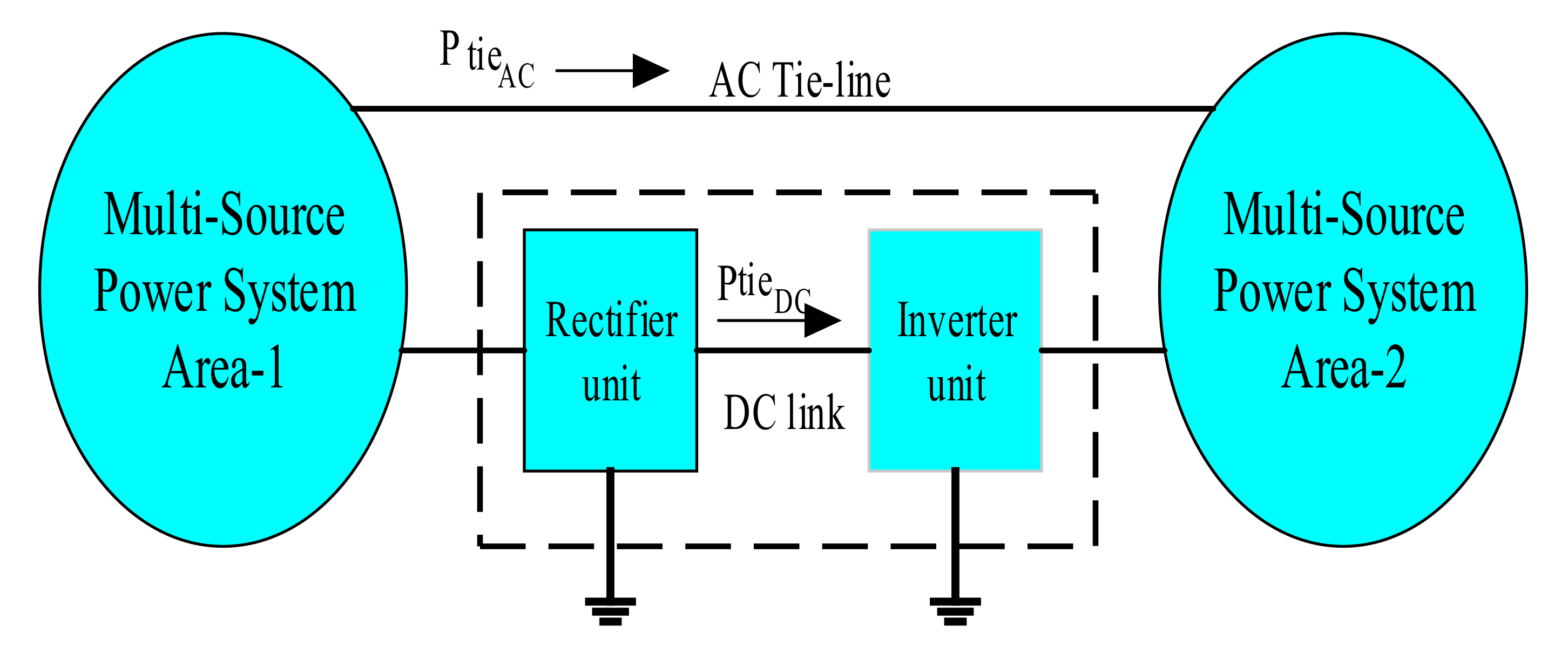
- Considering, the effect of HVDC links to eliminate the problems related to the AC links.
- iv.
- Considering load disturbance, renewable power penetration (i.e., wind power), and system parameters variations during designing the parameters of the proposed fuzzy-PID controller-based AOA algorithm.
- v.
- Comparing the performance of the AOA algorithm with other optimization algorithms such as differential evolution (DE) and teaching-learning based optimization (TLBO) for selecting the parameters of the PID controller in hybrid two-area power system.
- vi.
- Comparing the performance of the proposed control strategy with other techniques performances such as; PID controller-based differential evolution (PID-DE) [49], PID controller-based teaching-learning based optimization (PID-TLBO) [50], and fuzzy-PID controller-based a hybrid local unimodal sampling (LUS) with TLBO (Fuzzy-PID-LUS-TLBO) [50] in order to ensure the effectiveness and robustness of the proposed controller.
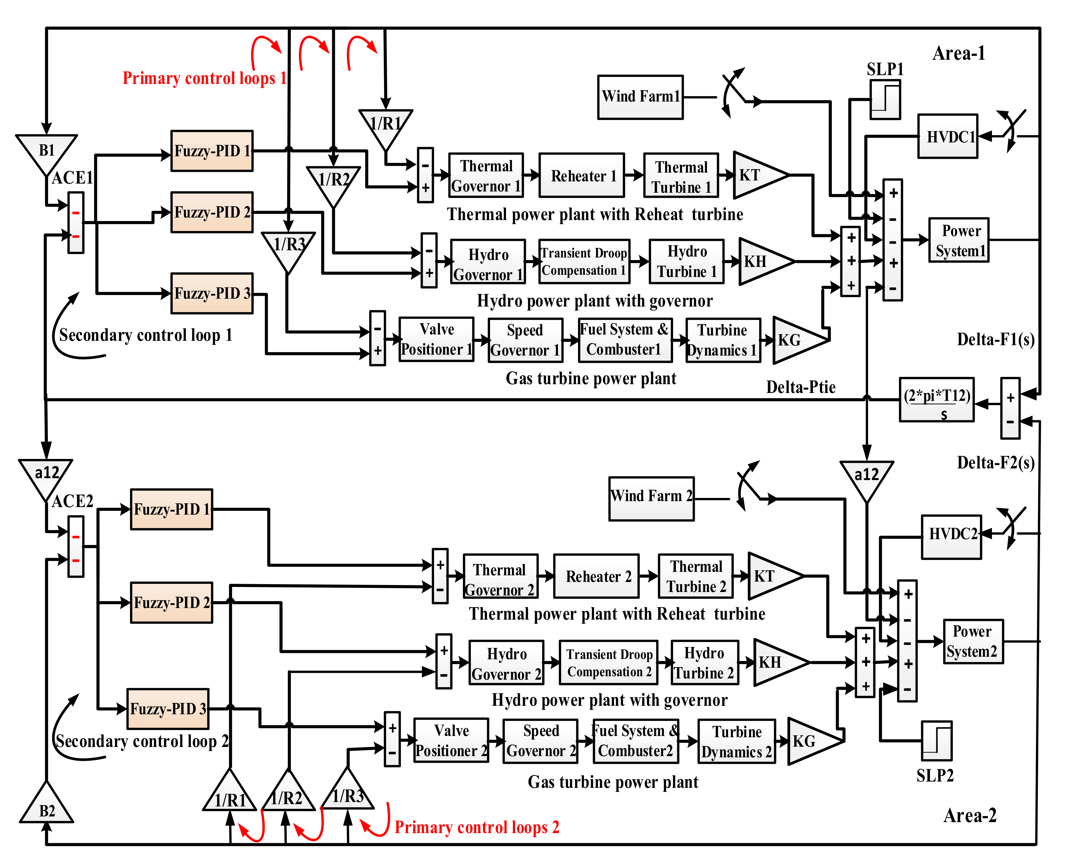
2. Modeling and Configuration of the Studied System
2.1. A dynamic Model of Two-Area Interconnected Power System
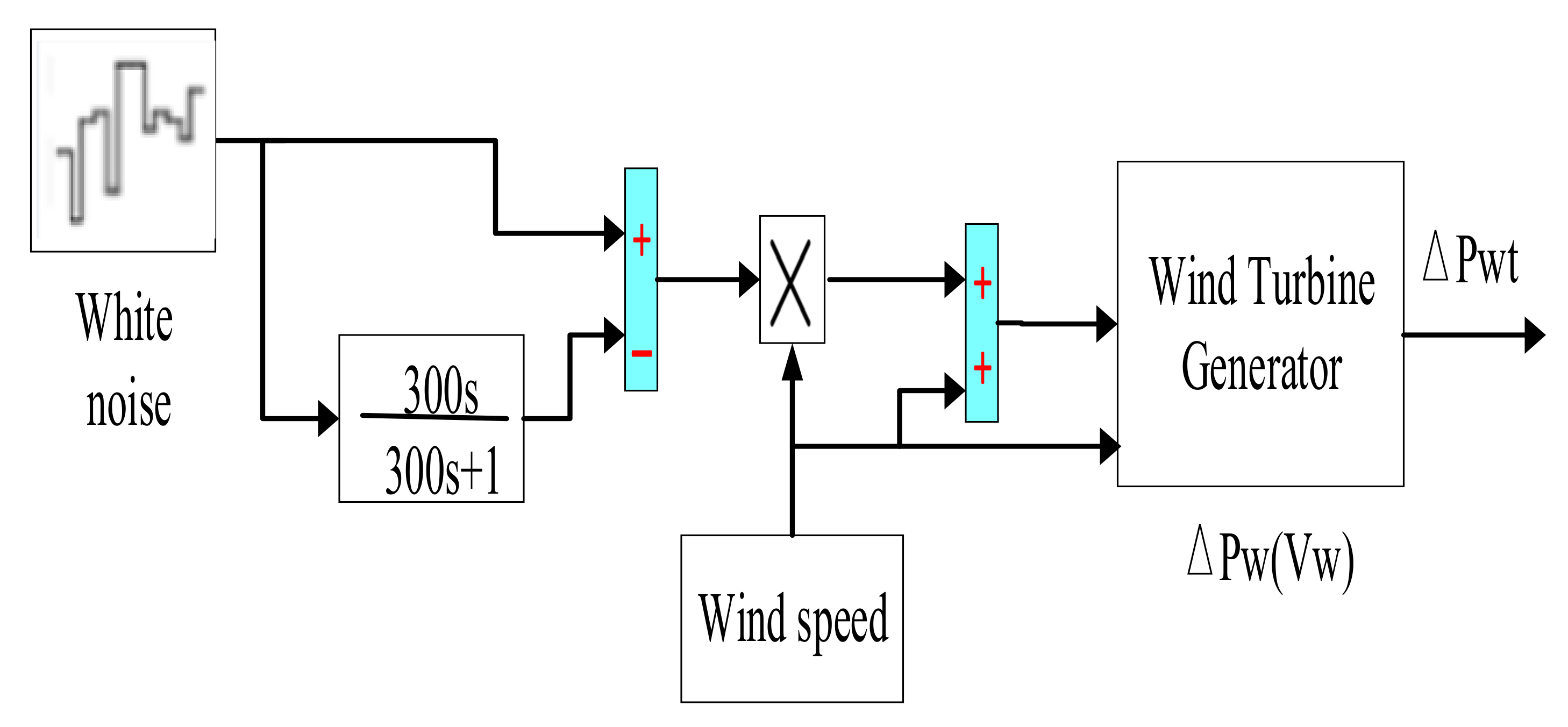
2.2. The Wind Farm Configuration
3. Control Methodology and Problem Formulation
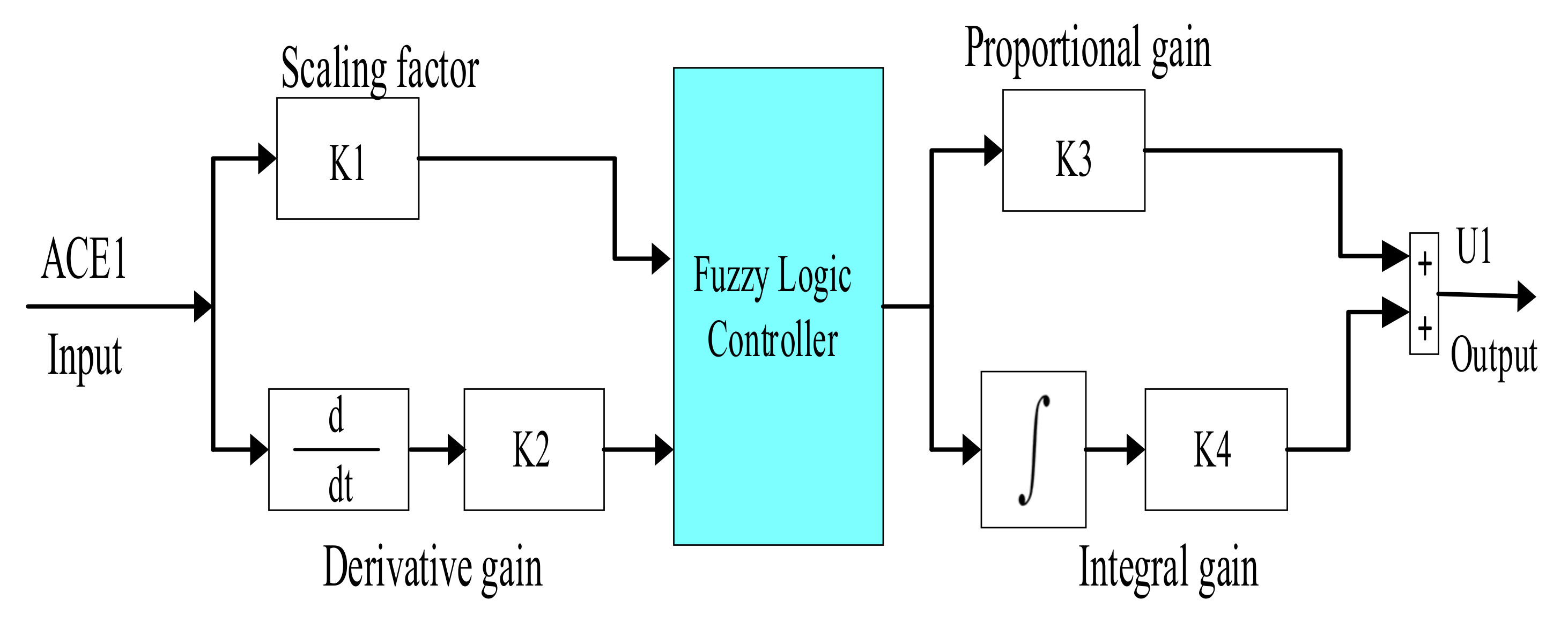
3.1. The Proposed Control Strategy
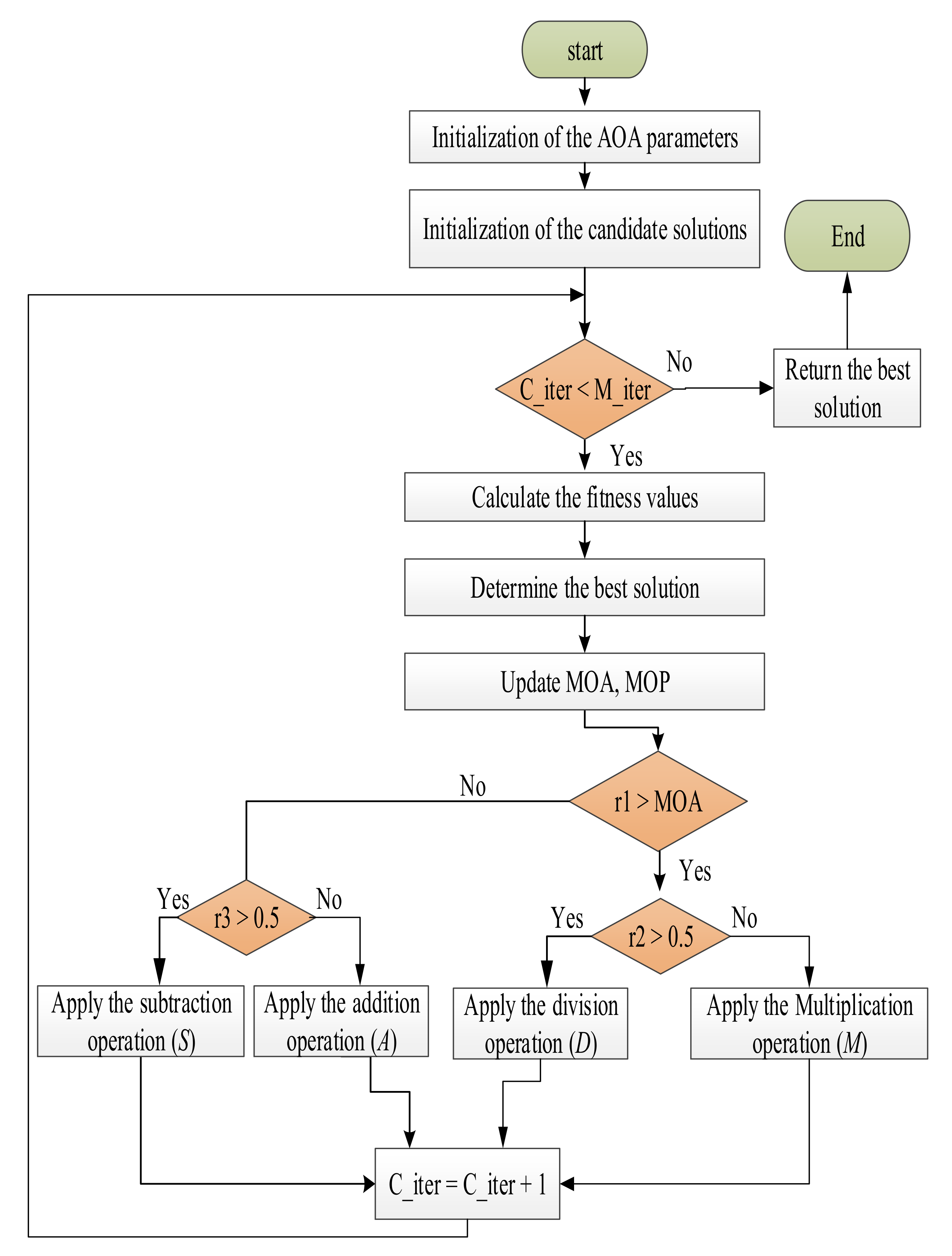
3.2. The Proposed Optimization Technique (AOA)
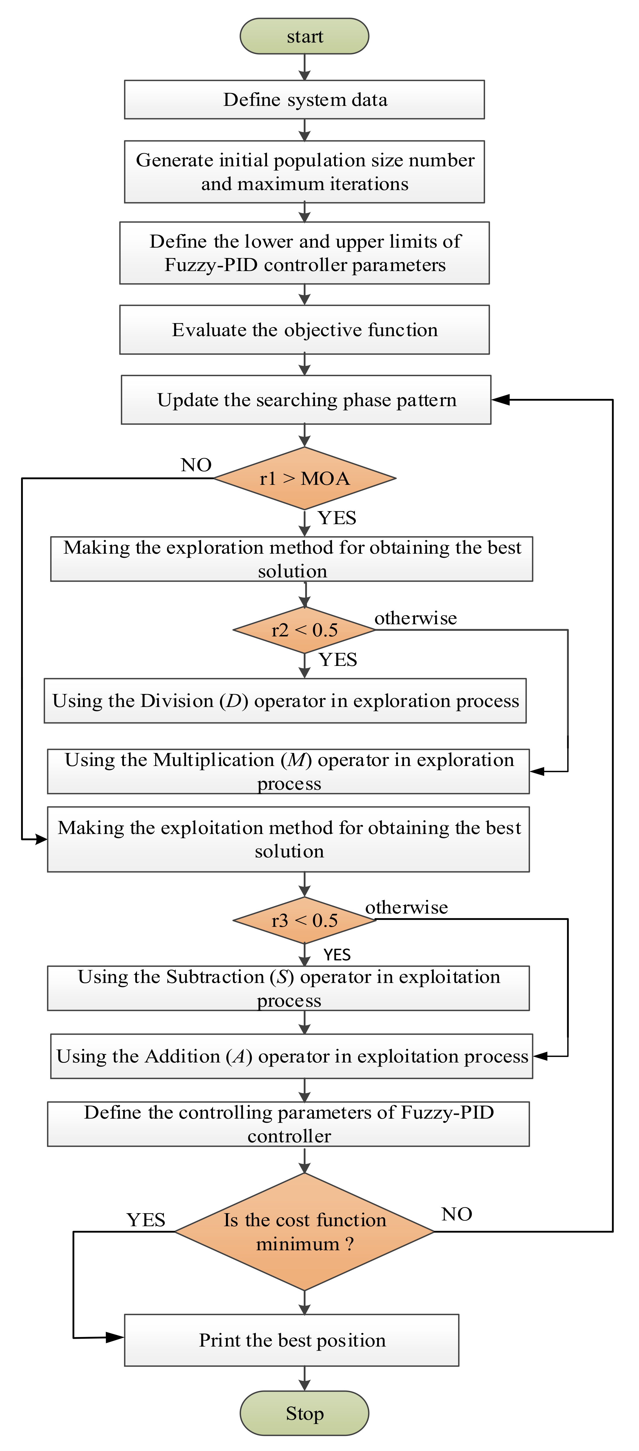
3.3. The Proposed Fuzzy-PID Control Strategy Based AOA Algorithm
4. Discussion and Simulation Results
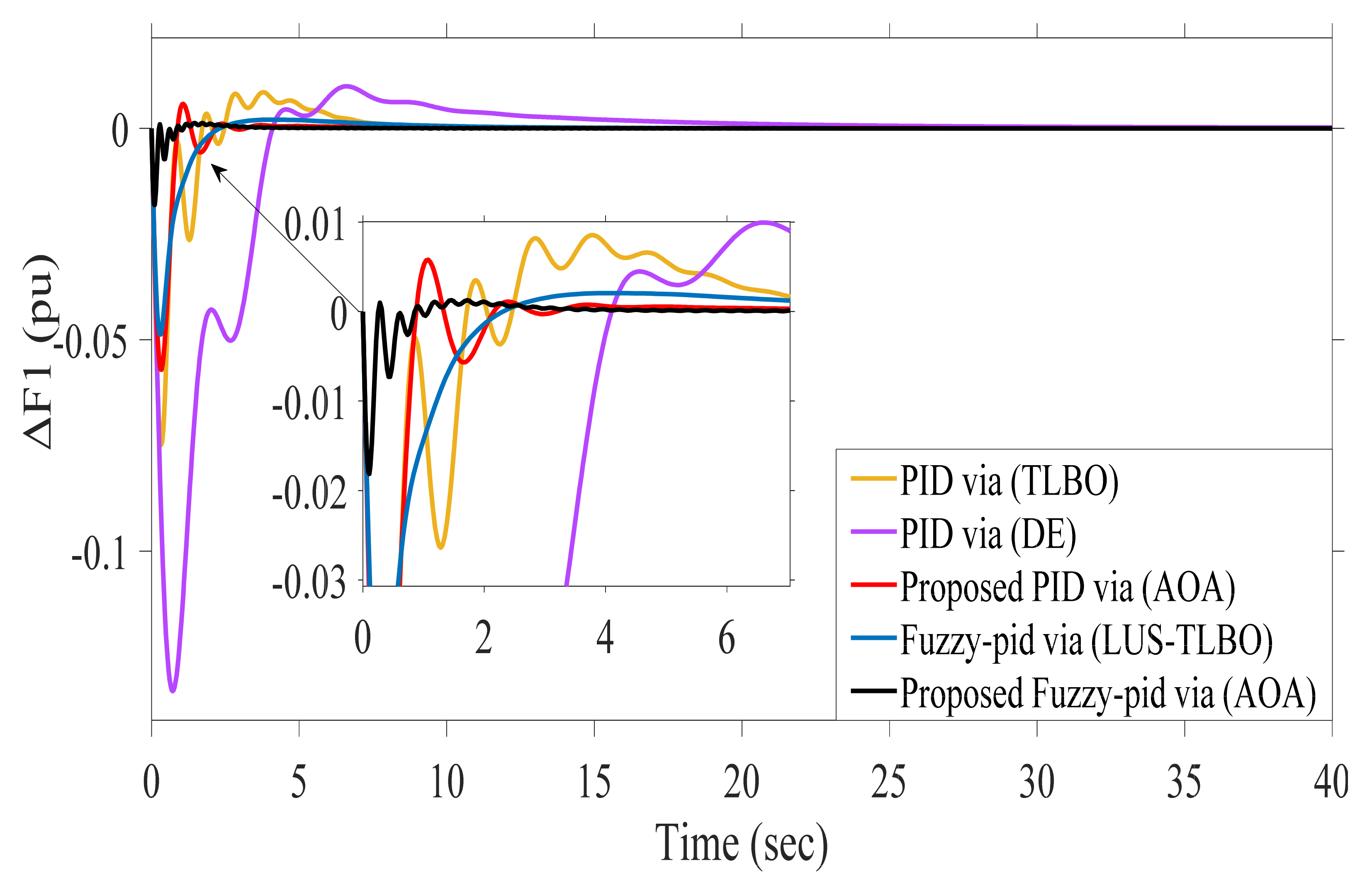
4.1. Studied Power System Performance Considering AC-Lines Connection Only
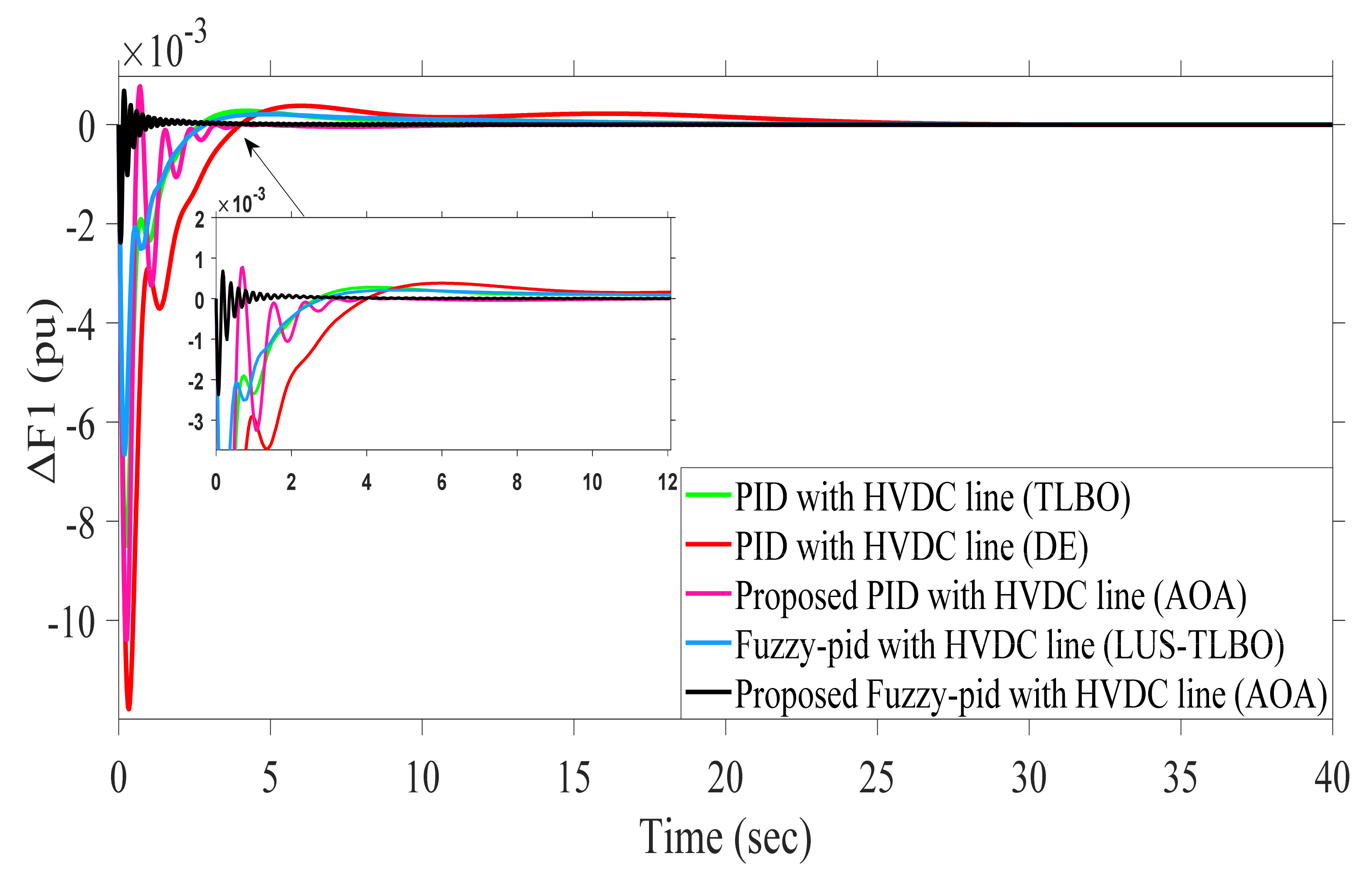
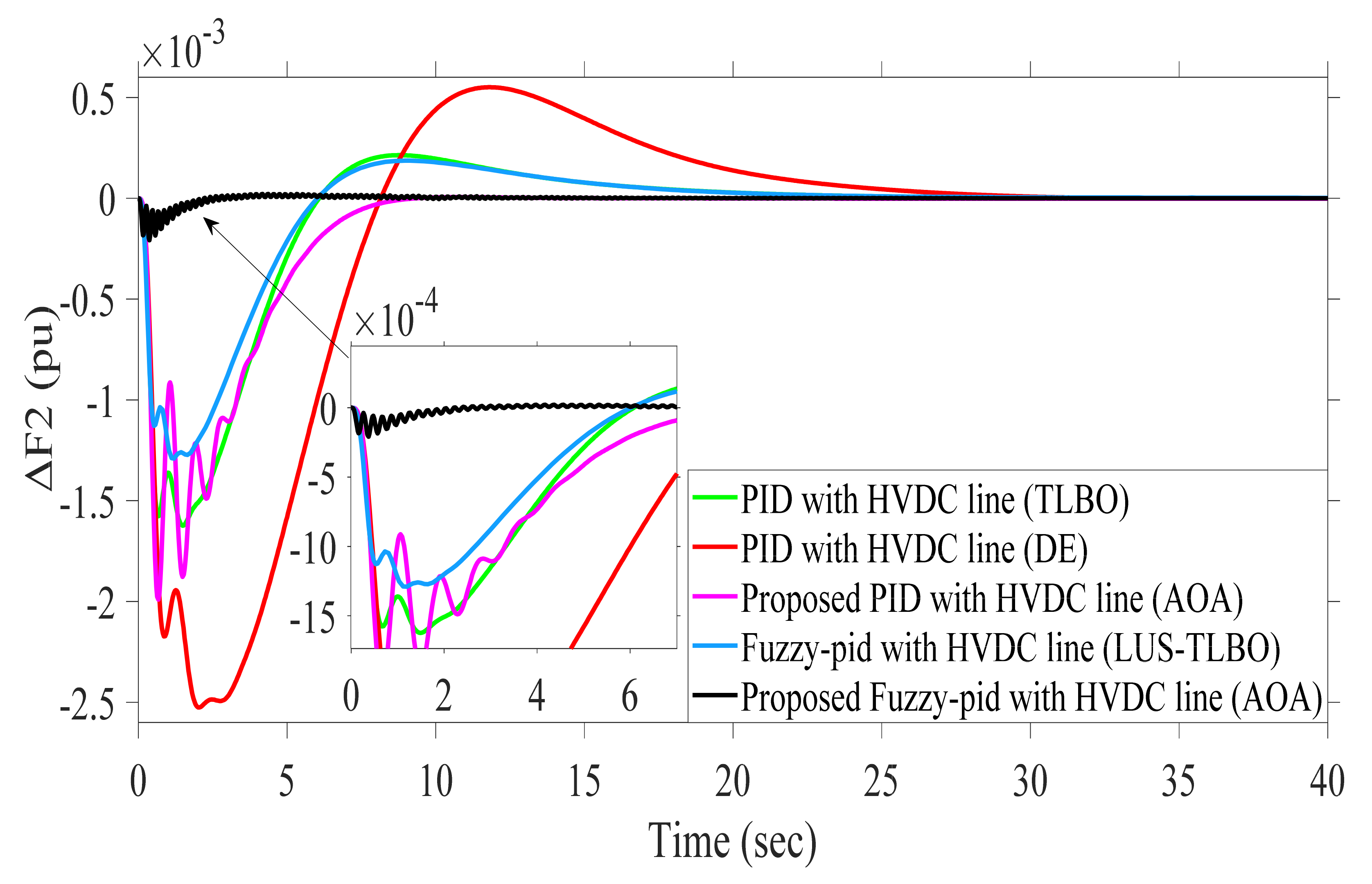
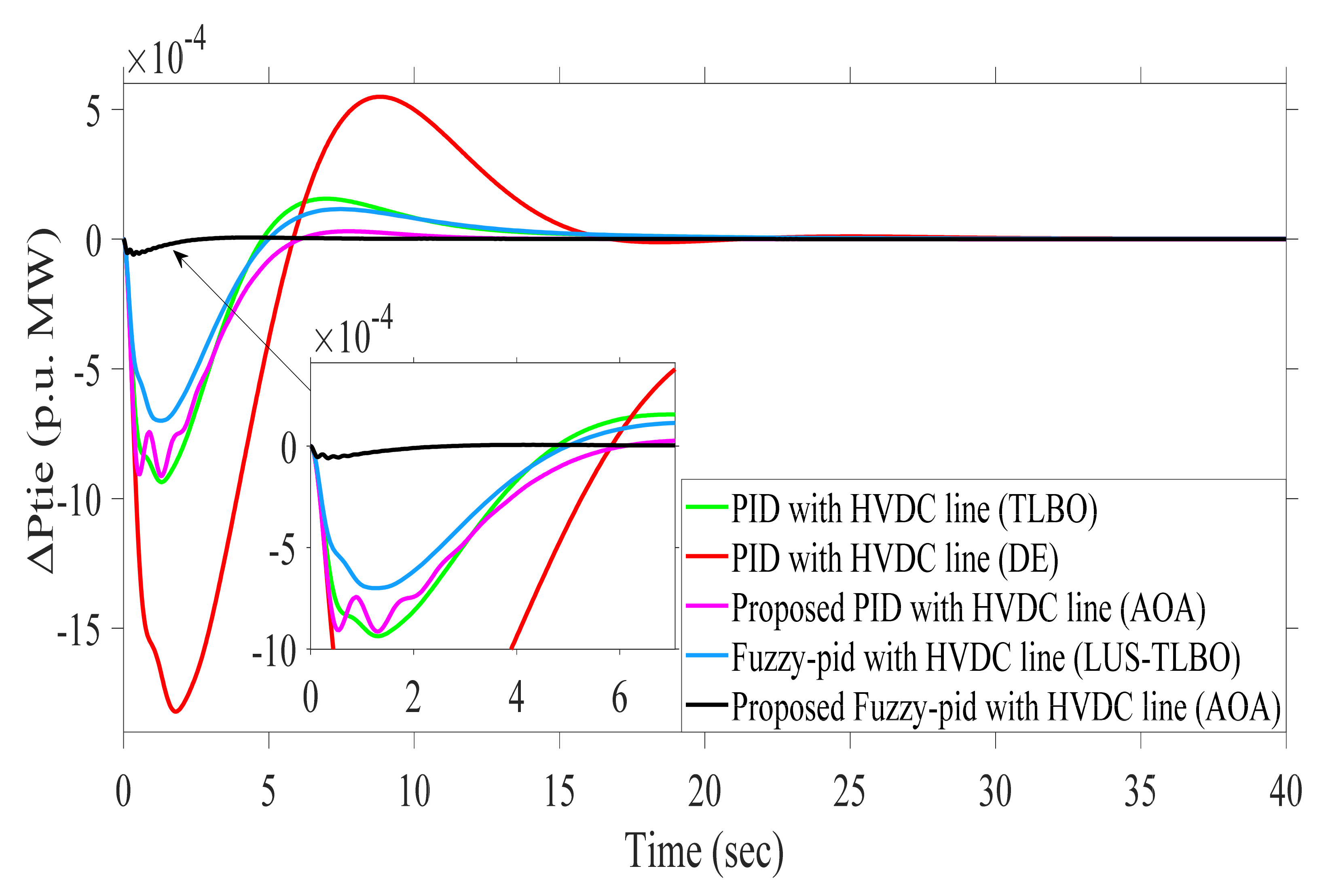
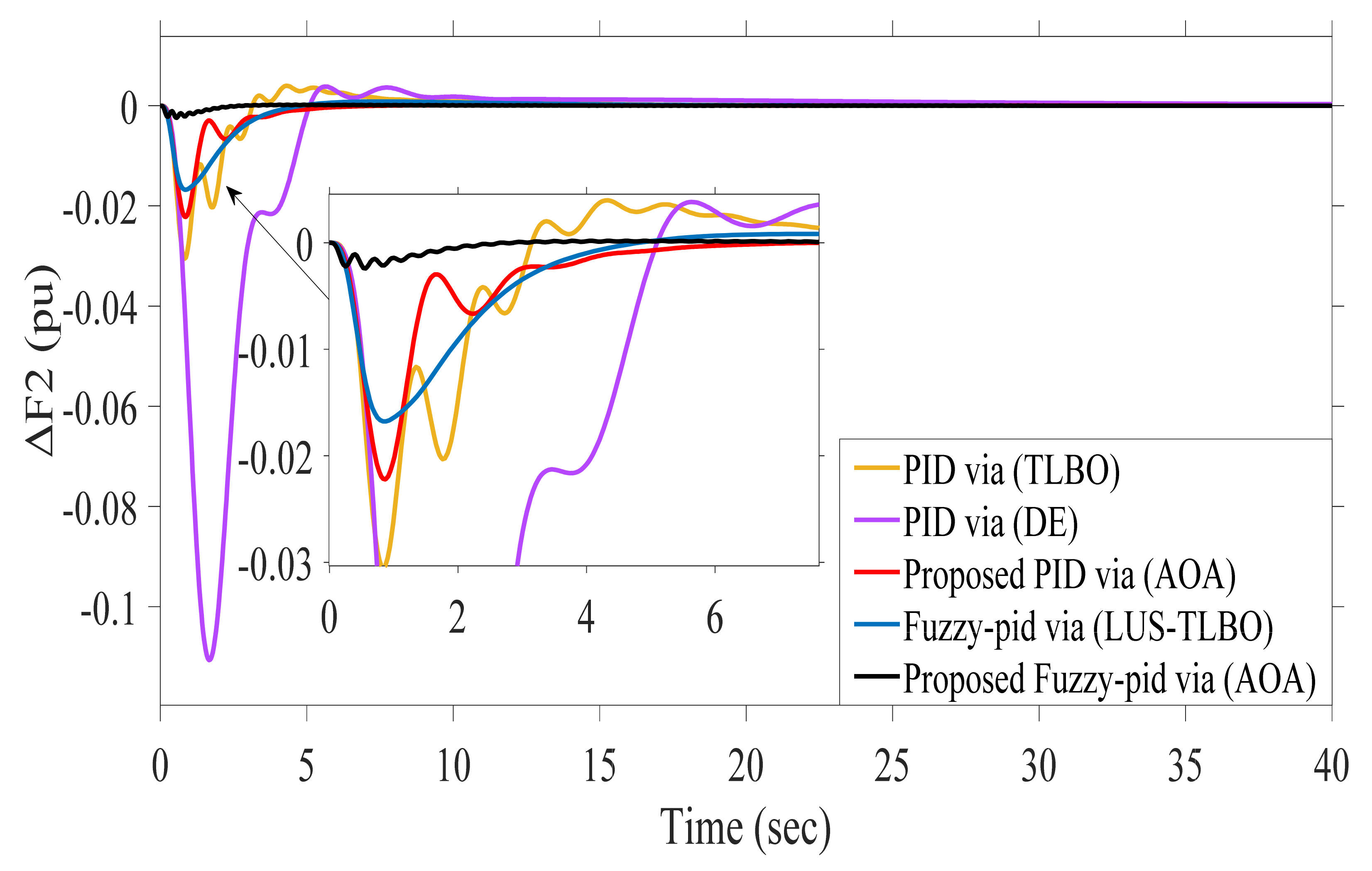
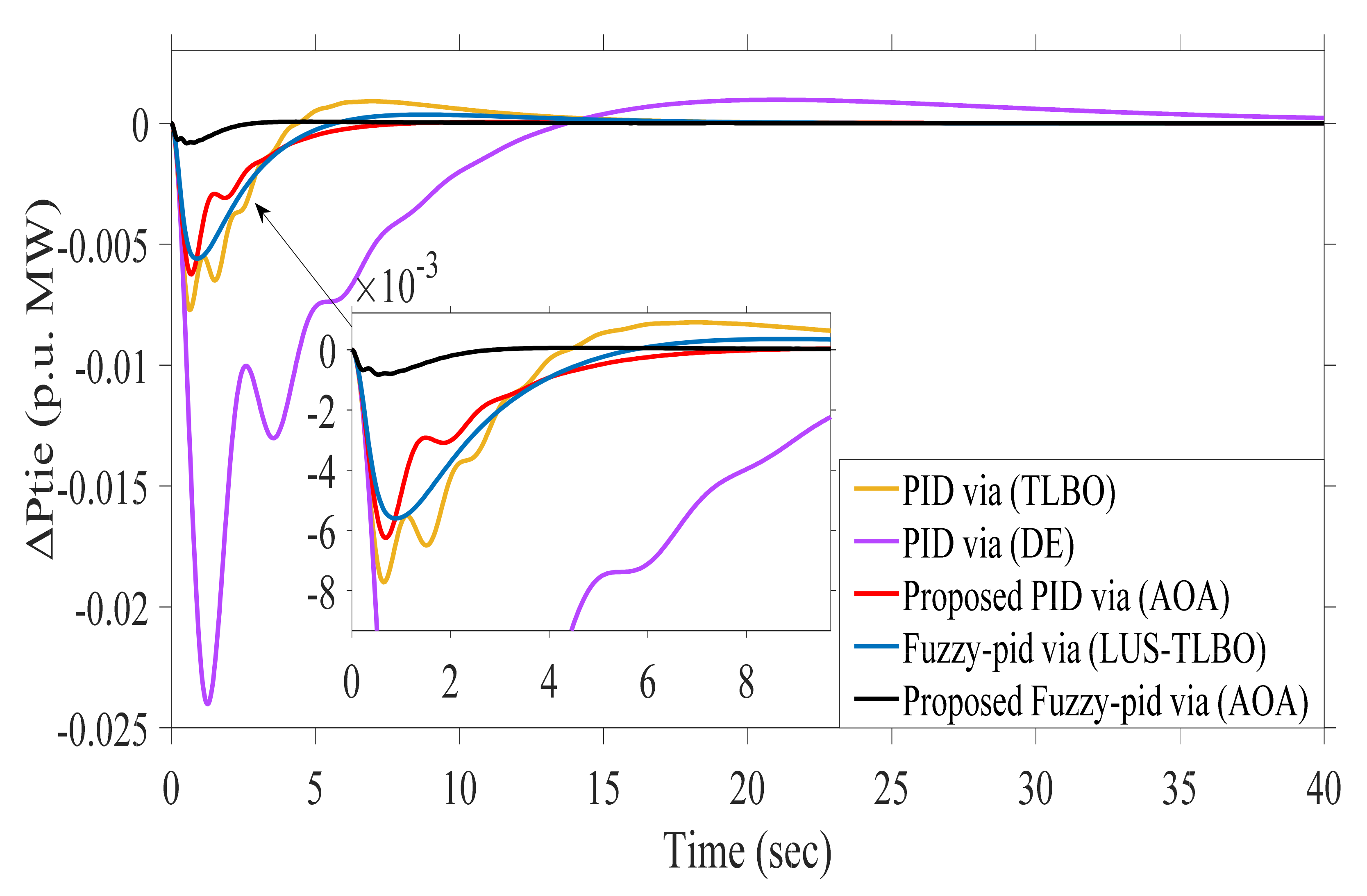
4.2. Studied Power System Performance Considering AC-DC Lines Connection
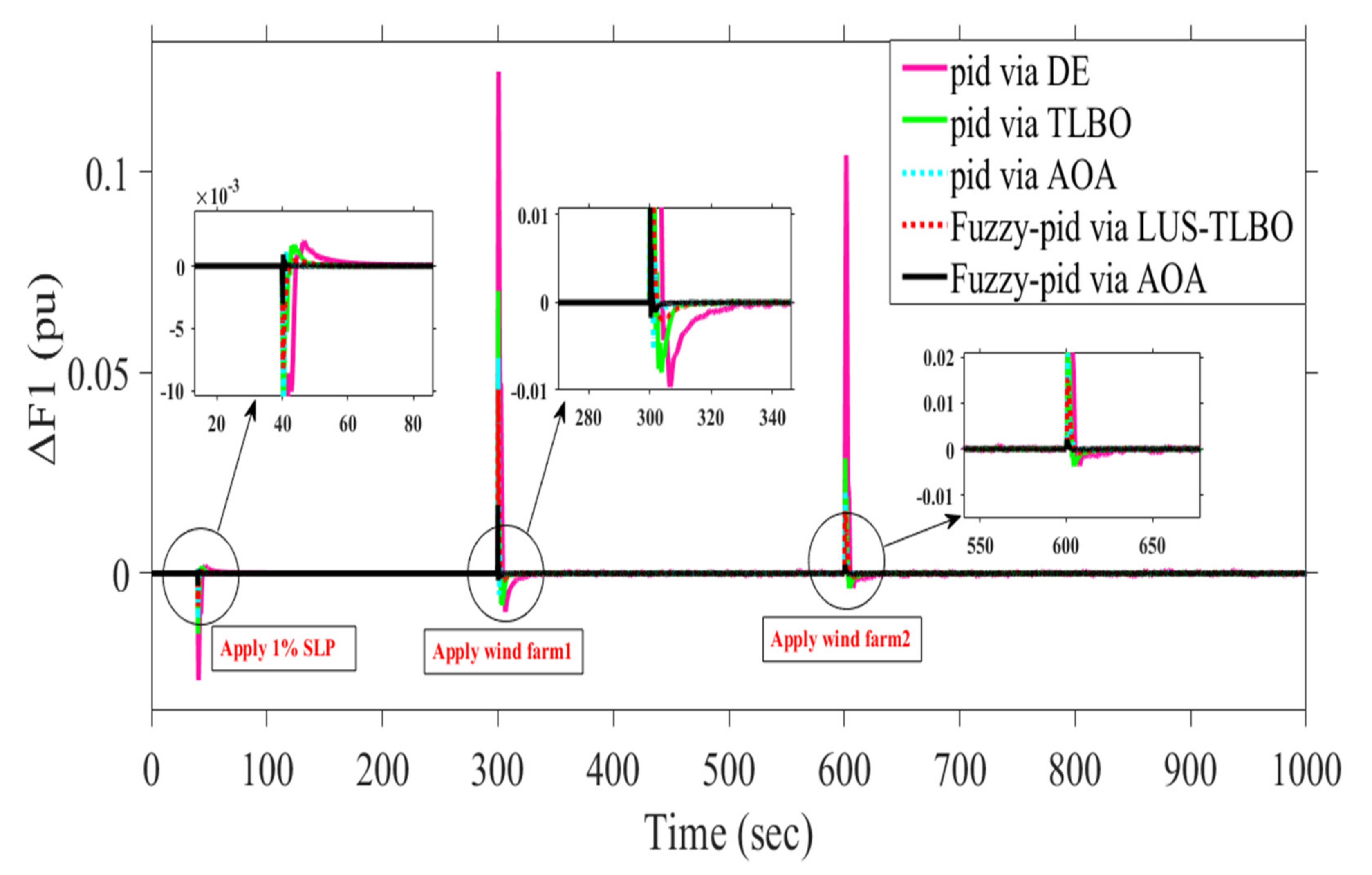
4.3. Studied Power System Performance Considering AC-DC Lines Connection in Addition to Different Load Disturbances
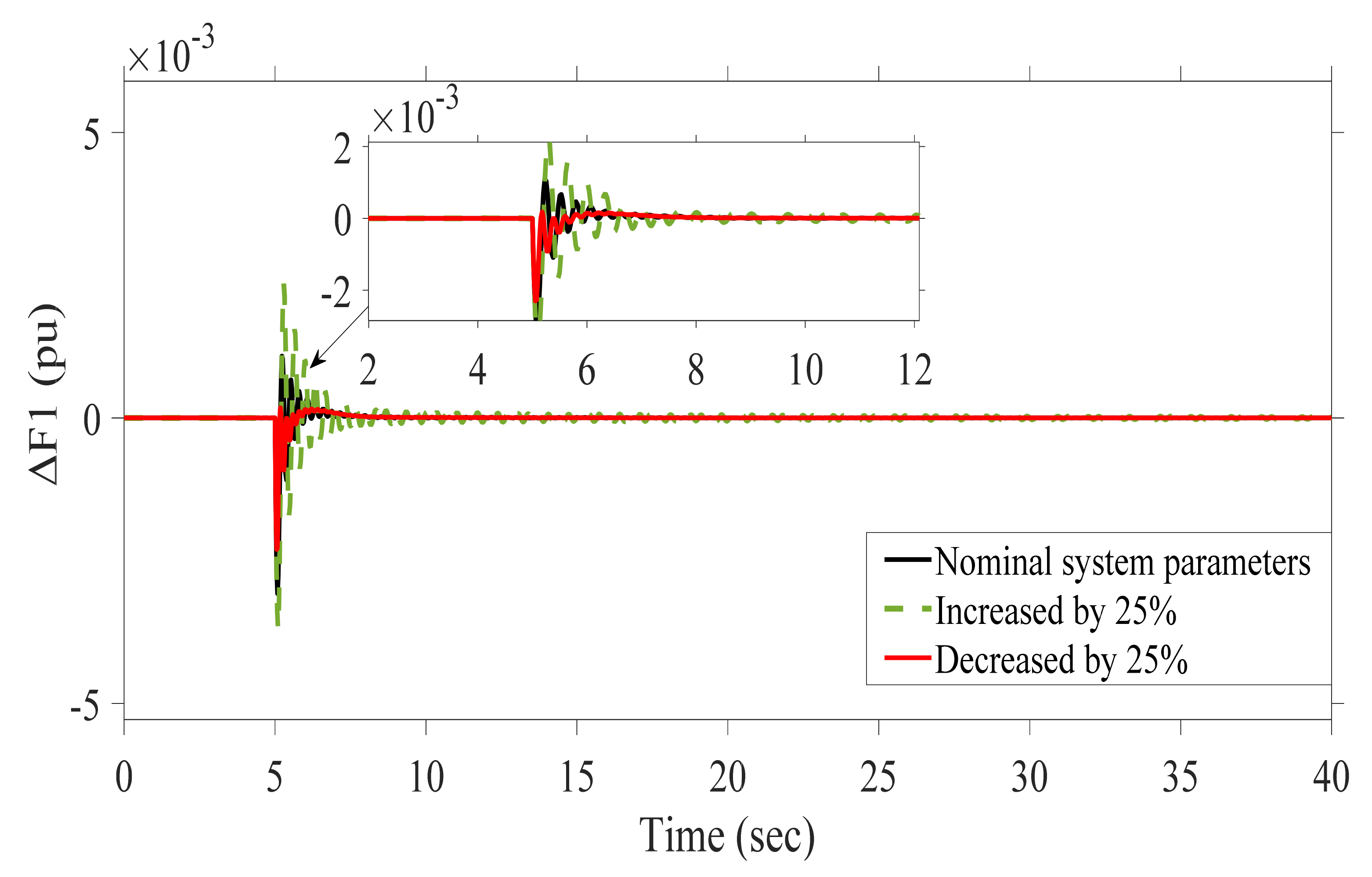
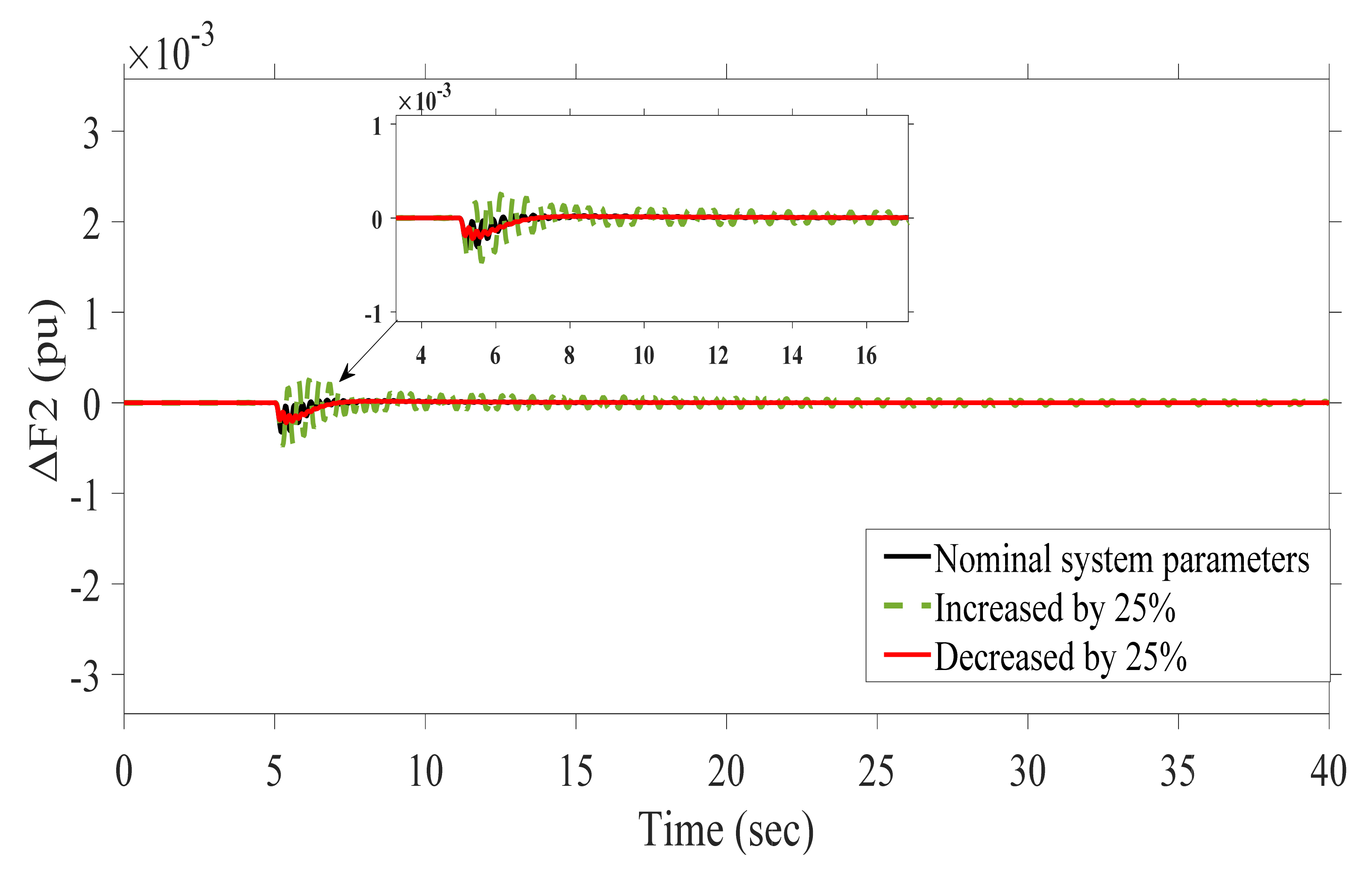
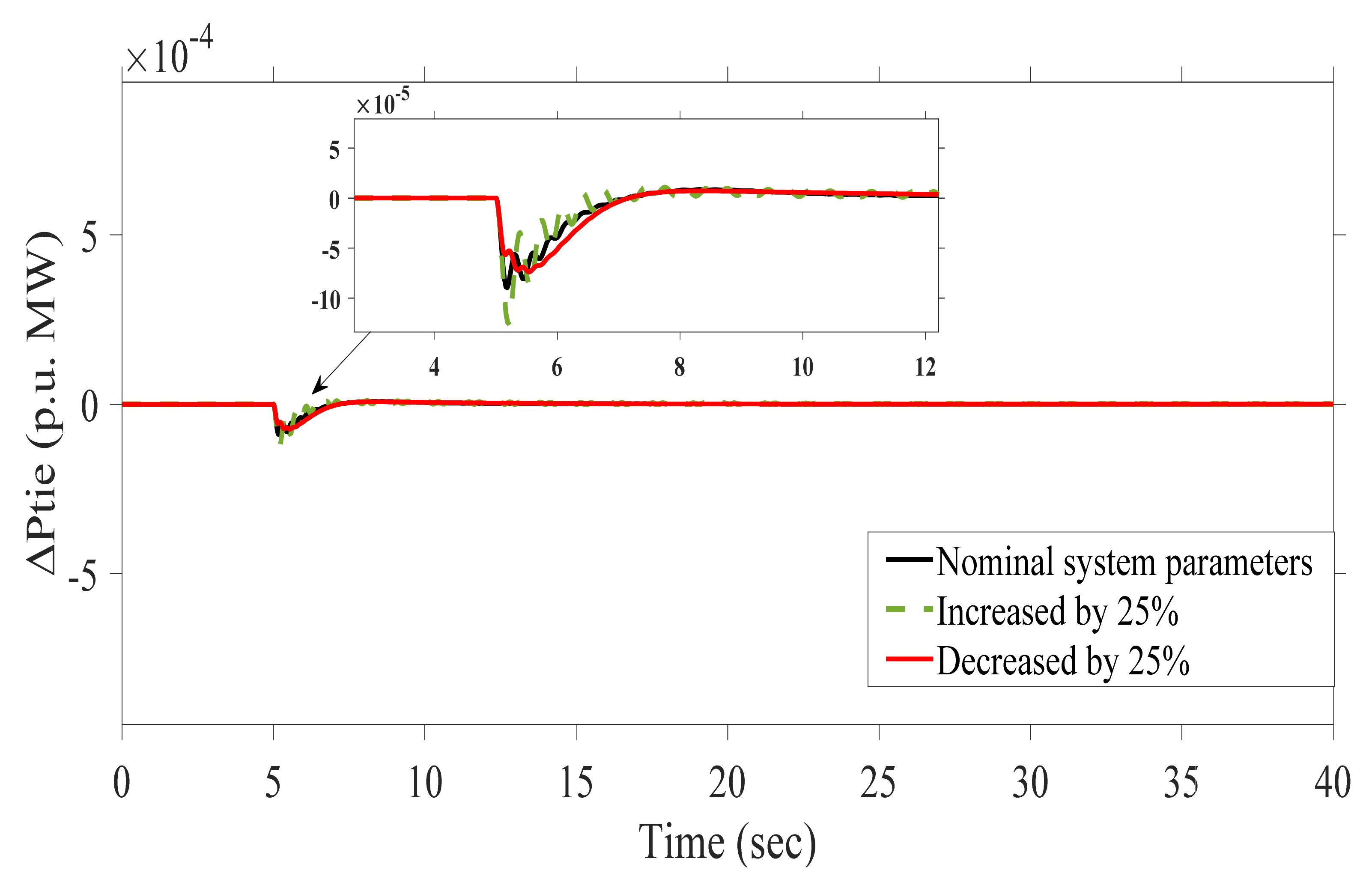
4.4. Studied Power System Performance Considering the Effect of System Parameters’ Variations
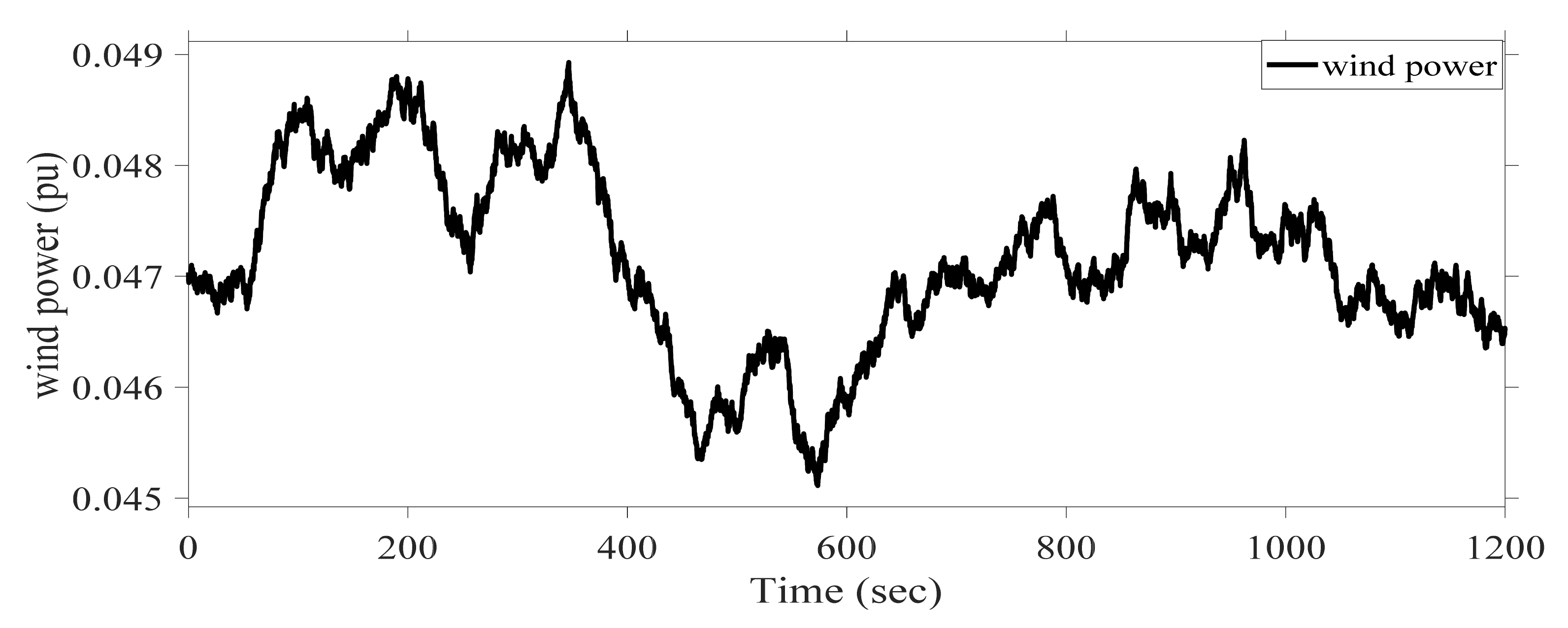
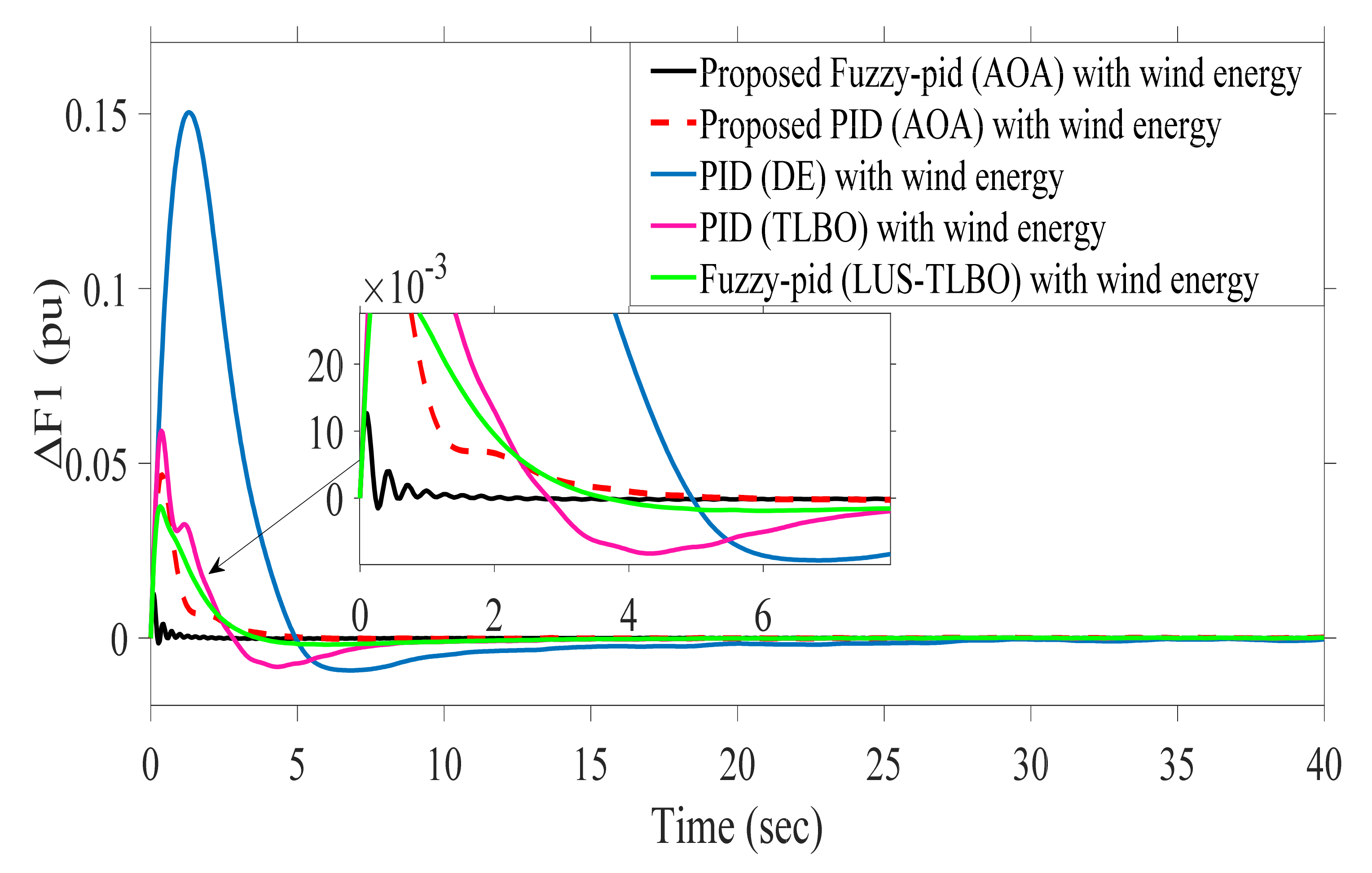
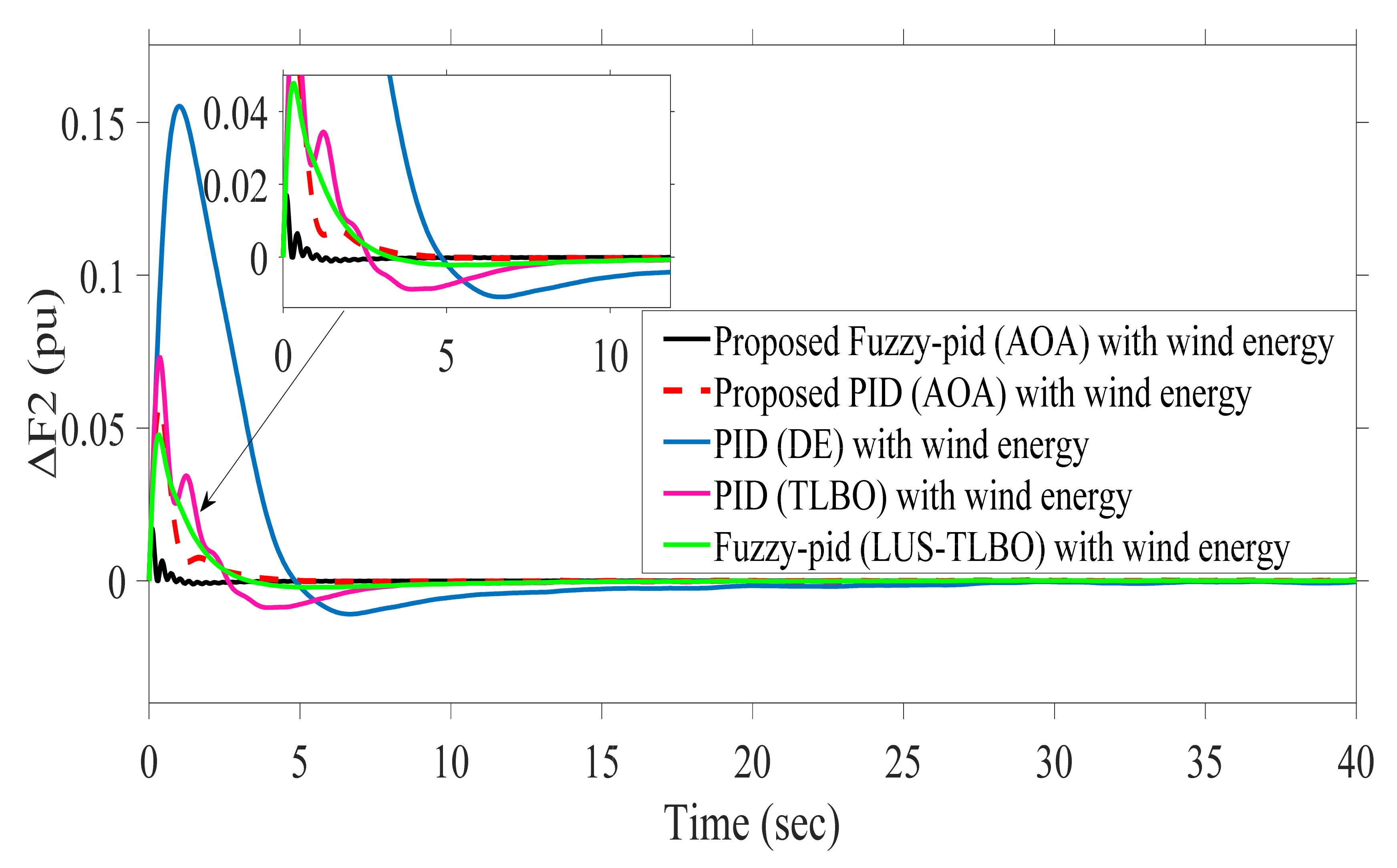
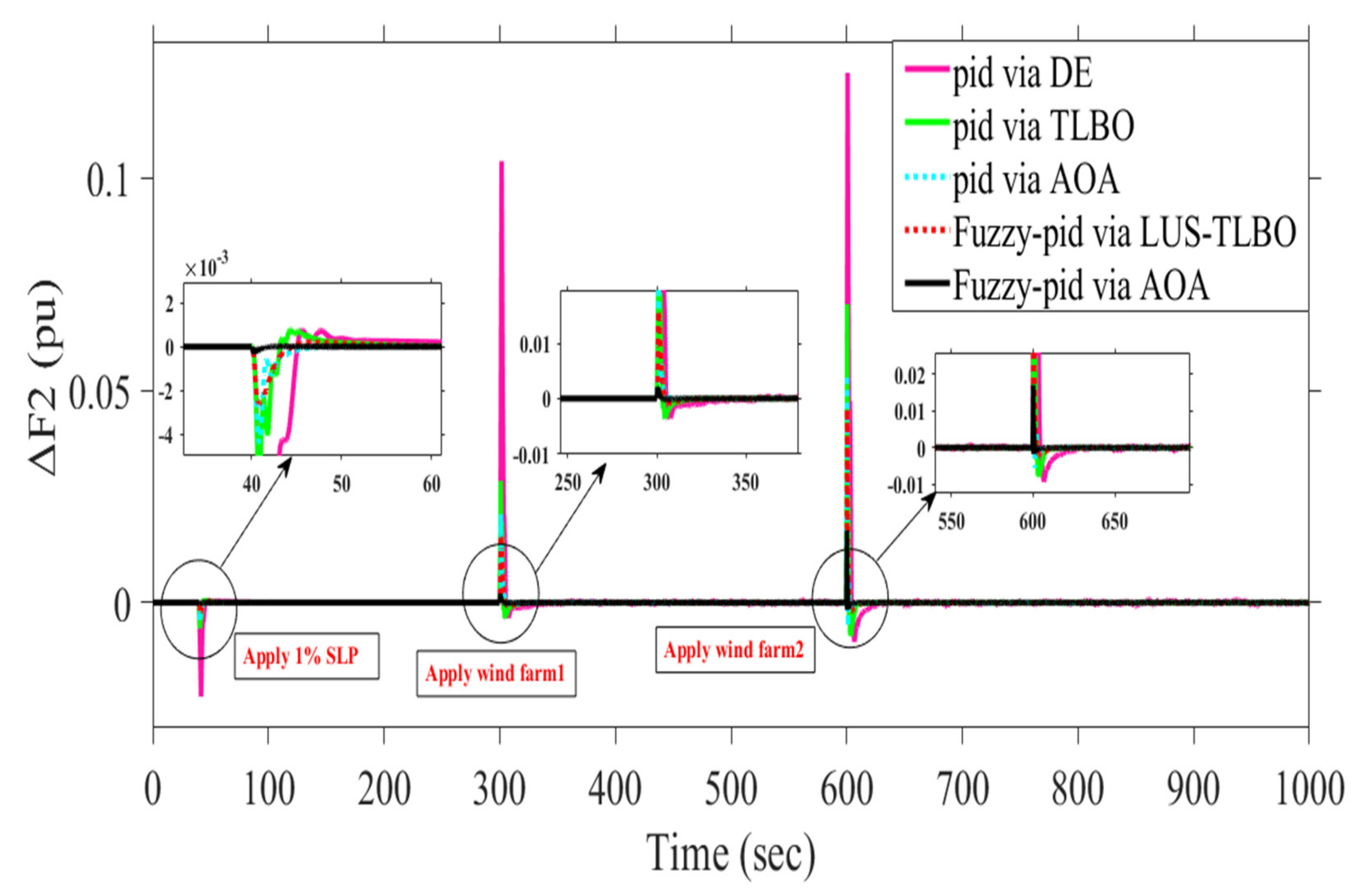
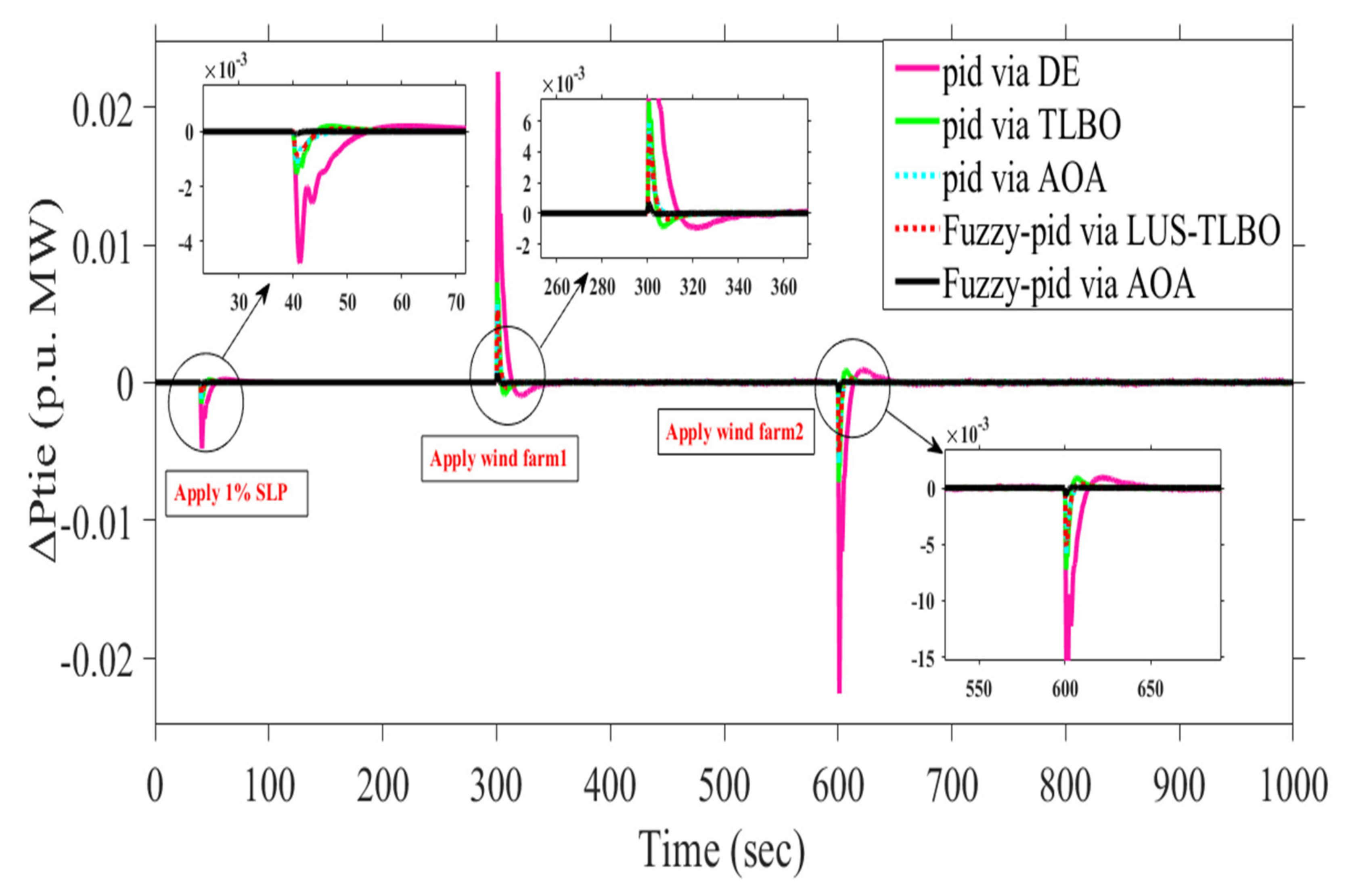
4.5. Studied Power System Performance Considering Wind Power Penetration
4.5.1. Case A
4.5.2. Case B
5. Conclusions
- The proposed fuzzy-PID controller has been implemented on the two-area interconnected multi-source power systems that include thermal, hydro, and gas power plants for tackling the LFC problem.
- The selection the of the proposed controller parameters has been made via a new meta-heuristic optimization technique, which is known as an arithmetic optimization algorithm, to get the optimal solution which leads to stabilizing the system performance. Appling HVDC link in addition to AC links to overcome the demerits of the AC tie-lines.
- Considering several challenges during designing the proposed control parameters such as (i.e., system uncertainties, different load variations, and different levels of wind power penetration).
- Applying different scenarios to validate the robustness of the proposed fuzzy-PID controller than other previous controllers.
- The proposed AOA has tuned the fuzzy-PID controller to achieve a better disturbance rejection ratio than a newly published technique namely a hybrid Local Unimodal Sampling and Teaching Learning Based Optimization using also Fuzzy-PID controller. On the other hand, PID controller-based-AOA gets more system stability than which utilized in previous research work optimized by Differential Evolution, TLBO.
- The system performance has been enhanced by 90.76% by applying the proposed fuzzy-PID controller based on the AOA algorithm in comparison with the fuzzy-PID controller based on the LUS-TLBO algorithm.
- The presence of an HVDC link in parallel with an AC link improved system performance by 95.42% when compared to using only an AC tie-line.
- According to the analysis and simulation results, the Fuzzy-PID controller based on the AOA algorithm gives better results in terms of system stability and security in comparison with other previous control techniques.
- Increasing the penetration level of renewable energy sources in the considered system.
- Applying different types of energy storage devices to study its effect on LFC problem.
- Improving of different recent optimization techniques to achieve the desired control parameters that lead to satisfied performance.
Author Contributions
Funding
Institutional Review Board Statement
Informed Consent Statement
Data Availability Statement
Acknowledgments
Conflicts of Interest
Nomenclature
| Symbols | Parameters |
| FLC | Fuzzy logic control |
| PID | Proportional-Integral-Derivative |
| AOA | Arithmetic Optimization Algorithm |
| LFC | Load Frequency Control |
| HVDC | High Voltage Direct Current |
| RESs | Renewable Energy Sources |
| CESs | Conventional Energy Sources |
| DE | Differential Evolution |
| LUS | Local Unimodal Sampling |
| TLBO | Teaching Learning-based Optimization |
| OS | overshoot |
| US | undershoot |
| SLP | Step load perturbation |
| Wind turbine output power | |
| ρ | The air density |
| The swept area by the blades of turbine | |
| The wind speed | |
| The coefficient of rotor blades | |
| – | The turbine coefficients |
| β | The pitch angle |
| The radius of rotor | |
| The rotor speed | |
| The optimum tip-speed ratio | |
| The intermittent tip-speed ratio | |
| Frequency bias factor of Area 1 | |
| Frequency bias factor of Area 2 | |
| Deviation in frequency waveform in area 1 | |
| Deviation in frequency waveform in area 2 | |
| Tie-line power exchange at area 1 | |
| Tie-line power exchange at area 2 | |
| Coefficient of synchronizing | |
| Regulation constant of thermal power plant | |
| Regulation constant of hydro power plant | |
| Regulation constant of gas turbine | |
| Control Area Capacity Ratio | |
| Participation factor for thermal unit | |
| Participation factor for hydro unit | |
| Participation factor for gas unit | |
| Gain constant of power system | |
| Time constant of power system | |
| Governor time constant | |
| Turbine Time Constant | |
| Gain of reheater steam turbine | |
| Time Constant of reheater steam turbine | |
| Speed governor time constant of hydro turbine | |
| Speed governor reset time of hydro turbine | |
| Transient droop time constant of hydro turbine speed governor | |
| Nominal string time of water in penstock | |
| Gas turbine constant of valve positioner | |
| Valve positioner of gas turbine | |
| Lag time constant of gas turbine speed governor | |
| Lead time constant of gas turbine speed governor | |
| Gas turbine combustion reaction time delay | |
| Gas turbine fuel time constant | |
| Gas turbine compressor discharge volume-time constant | |
| Gain of HVDC link | |
| Time constant of hvdc link | |
| ITAE | Integral time absolute error |
| ISE | Integral square error |
| IAE | Integral absolute error |
| Input scaling factor | |
| Derivative input gain | |
| Proportional output gain | |
| Integral output gain | |
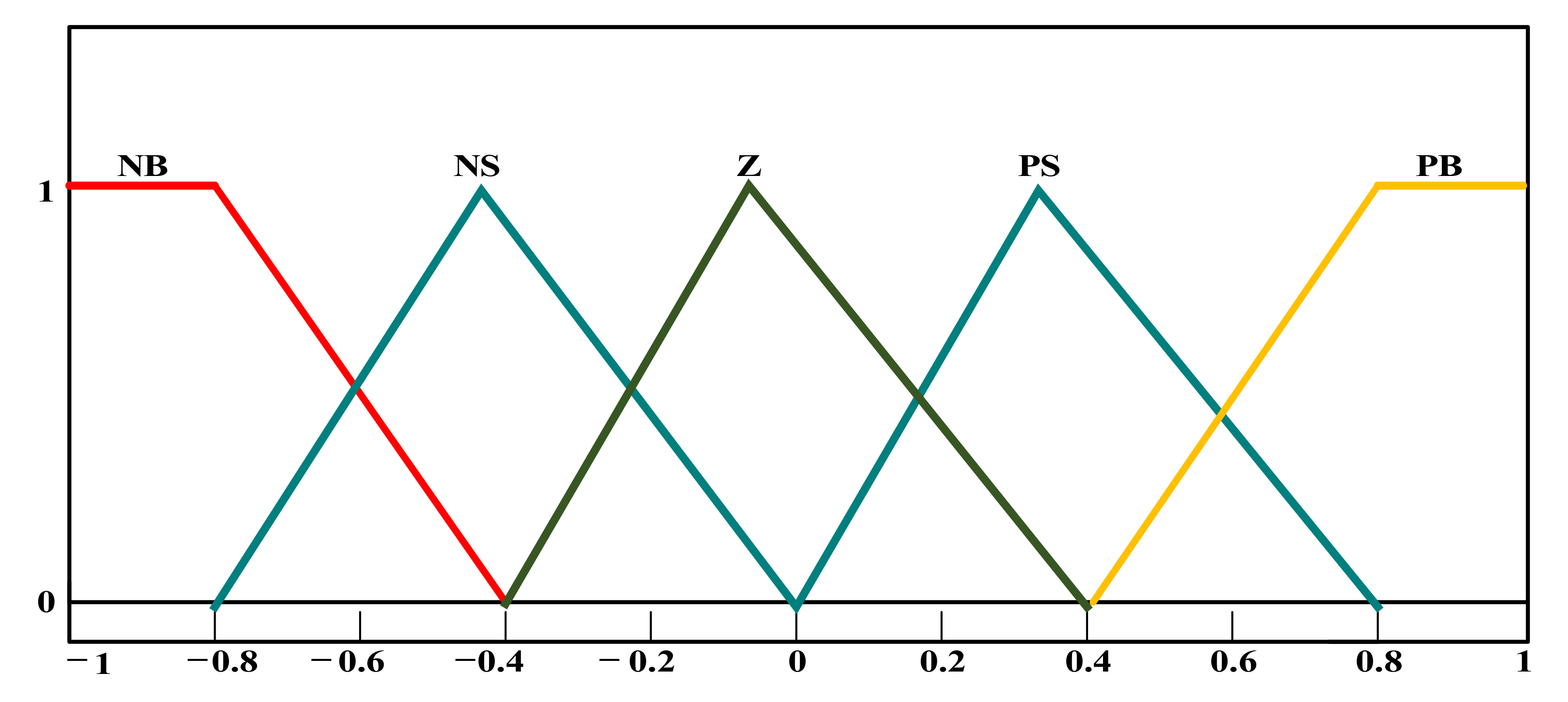
| NB | Negative big |
| NS | Negative small |
| Z | Zero |
| PB | Positive big |
| PS | Positive small |
| UB | Upper boundary value |
| LB | Lower boundary value |
Appendix A

| Control Block | Transfer Functions |
|---|---|
| Thermal Governor | |
| Reheater of Thermal Turbine | |
| Thermal Turbine | |
| Hydro Governor | |
| Transient Droop Compensation | |
| Hydro Turbine | |
| Valve Positioner of Gas Turbine | |
| Speed Governor of Gas Turbine | |
| Fuel System and Combustor | |
| Gas Turbine Dynamics | |
| Power System 1 | |
| Power System 2 | |
| HVDC 1 | |
| HVDC 2 |
References
- Mosaad, M.I.; El-Raouf, M.O.A.; Al-Ahmar, M.A.; Bendary, F.M. Optimal PI controller of DVR to enhance the performance of hybrid power system feeding a remote area in Egypt. Sustain. Cities Soc. 2019, 47, 101469. [Google Scholar] [CrossRef]
- Balu, N.J.; Lauby, M.G.; Kundur, P. Power System Stability and Control; Electrical Power Research Institute, McGraw-Hill Professional: Washington, DC, USA, 1994. [Google Scholar]
- Omer, A.M. Energy, environment and sustainable development. Renew. Sustain. Energy Rev. 2008, 12, 2265–2300. [Google Scholar] [CrossRef]
- Bilgen, S.; Kaygusuz, K.; Sari, A. Renewable Energy for a Clean and Sustainable Future. Energy Sources 2004, 26, 1119–1129. [Google Scholar] [CrossRef]
- Blaabjerg, F.; Teodorescu, R.; Liserre, M.; Timbus, A. Overview of Control and Grid Synchronization for Distributed Power Generation Systems. IEEE Trans. Ind. Electron. 2006, 53, 1398–1409. [Google Scholar] [CrossRef] [Green Version]
- Fang, J.; Li, H.; Tang, Y.; Blaabjerg, F. Distributed Power System Virtual Inertia Implemented by Grid-Connected Power Converters. IEEE Trans. Power Electron. 2017, 33, 8488–8499. [Google Scholar] [CrossRef] [Green Version]
- Bevrani, H. Robust Power System Frequency Control; Springer: Berlin/Heidelberg, Germany, 2009. [Google Scholar]
- Shahalami, S.H.; Farsi, D. Analysis of Load Frequency Control in a restructured multi-area power system with the Kalman filter and the LQR controller. AEU-Int. J. Electron. Commun. 2018, 86, 25–46. [Google Scholar] [CrossRef]
- Das, S.K.; Rahman, M.; Paul, S.K.; Armin, M.; Roy, P.N.; Paul, N. High-Performance Robust Controller Design of Plug-In Hybrid Electric Vehicle for Frequency Regulation of Smart Grid Using Linear Matrix Inequality Approach. IEEE Access 2019, 7, 116911–116924. [Google Scholar] [CrossRef]
- Liao, K.; Xu, Y. A Robust Load Frequency Control Scheme for Power Systems Based on Second-Order Sliding Mode and Extended Disturbance Observer. IEEE Trans. Ind. Inform. 2018, 14, 3076–3086. [Google Scholar] [CrossRef]
- HBevrani, H.; Feizi, M.R.; Ataee, S. Robust Frequency Control in an Islanded Microgrid: H∞ and μ-Synthesis Approaches. IEEE Trans. Smart Grid 2015, 7, 706–717. [Google Scholar] [CrossRef] [Green Version]
- Wang, Z.-Q.; Sznaier, M. Robust control design for load frequency control using/spl mu/-synthesis. In Proceedings of the SOUTHCON’94, Orlando, FL, USA, 29–31 March 1994; pp. 186–190. [Google Scholar]
- Wang, Y.; Zhou, R.; Gao, L. H/sub ∞/controller design for power system load frequency control. In Proceedings of the TENCON’93, IEEE Region 10 International Conference on Computers, Communications and Automation, Beijing, China, 19–21 October 1993. [Google Scholar]
- Ma, M.; Liu, X.; Zhang, C. LFC for multi-area interconnected power system concerning wind turbines based on DMPC. IET Gener. Transm. Distrib. 2017, 11, 2689–2696. [Google Scholar] [CrossRef]
- Khooban, M.H.; Gheisarnejad, M. A Novel Deep Reinforcement Learning Controller Based Type-II Fuzzy System: Frequency Regulation in Microgrids. IEEE Trans. Emerg. Top. Comput. Intell. 2021, 5, 689–699. [Google Scholar] [CrossRef]
- Aluko, A.O.; Dorrell, D.G.; Pillay-Carpanen, R.; Ojo, E.E. Frequency Control of Modern Multi-Area Power Systems Using Fuzzy Logic Controller. In Proceedings of the 2019 IEEE PES/IAS PowerAfrica, Abuja, Nigeria, 20–23 August 2019. [Google Scholar]
- Yang, D.; Jin, E.; You, J.; Hua, L. Dynamic Frequency Support from a DFIG-Based Wind Turbine Generator via Virtual Inertia Control. Appl. Sci. 2020, 10, 3376. [Google Scholar] [CrossRef]
- Magdy, G.; Shabib, G.; Elbaset, A.A.; Mitani, Y. Renewable power systems dynamic security using a new coordination of frequency control strategy based on virtual synchronous generator and digital frequency protection. Int. J. Electr. Power Energy Syst. 2019, 109, 351–368. [Google Scholar] [CrossRef]
- Mudi, R.K.; Pal, N.R. A self-tuning fuzzy PI controller. Fuzzy Sets Syst. 2000, 115, 327–338. [Google Scholar] [CrossRef]
- Chang, C.; Fu, W. Area load frequency control using fuzzy gain scheduling of PI controllers. Electr. Power Syst. Res. 1997, 42, 145–152. [Google Scholar] [CrossRef]
- Yesil, E.; Güzelkaya, M.; Eksin, I. Self tuning fuzzy PID type load and frequency controller. Energy Convers. Manag. 2004, 45, 377–390. [Google Scholar] [CrossRef]
- Ahmadi, S.; Talami, S.H.; Sahnesaraie, M.A.; Dini, F.; Tahernejadjozam, B.; Ashgevari, Y. FUZZY aided PID controller is optimized by GA algorithm for Load Frequency Control of Multi-Source Power Systems. In Proceedings of the 2020 IEEE 18th World Symposium on Applied Machine Intelligence and Informatics (SAMI), Herlany, Slovakia, 23–25 January 2020. [Google Scholar]
- Lal, D.K.; Barisal, A.K. Comparative performances evaluation of FACTS devices on AGC with diverse sources of energy generation and SMES. Cogent Eng. 2017, 4, 1318466. [Google Scholar] [CrossRef]
- Lal, D.K.; Barisal, A.K.; Tripathy, M. Load Frequency Control of Multi Source Multi-Area Nonlinear Power System with DE-PSO Optimized Fuzzy PID Controller in Coordination with SSSC and RFB. Int. J. Control. Autom. 2018, 11, 61–80. [Google Scholar] [CrossRef]
- Lal, D.K.; Barisal, A.K.; Tripathy, M. Load Frequency Control of Multi Area Interconnected Microgrid Power System using Grasshopper Optimization Algorithm Optimized Fuzzy PID Controller. In Proceedings of the 2018 Recent Advances on Engineering, Technology and Computational Sciences (RAETCS), Allahabad, India, 6–8 February 2018. [Google Scholar]
- Dhanasekaran, B.; Siddhan, S.; Kaliannan, J. Ant colony optimization technique tuned controller for frequency regulation of single area nuclear power generating system. Microprocess. Microsyst. 2020, 73, 102953. [Google Scholar] [CrossRef]
- Annamraju, A.; Nandiraju, S. Coordinated control of conventional power sources and PHEVs using jaya algorithm optimized PID controller for frequency control of a renewable penetrated power system. Prot. Control. Mod. Power Syst. 2019, 4, 28. [Google Scholar] [CrossRef] [Green Version]
- Magdy, G.; Shabib, G.; Elbaset, A.A.; Kerdphol, T.; Qudaih, Y.; Mitani, Y. Decentralized optimal LFC for a real hybrid power system considering renewable energy sources. J. Eng. Sci. Technol. 2019, 14, 682–697. [Google Scholar]
- Khamari, D.; Kumbhakar, B.; Patra, S.; Laxmi, D.A.; Panigrahi, S. Load Frequency Control of a Single Area Power System using Firefly Algorithm. Int. J. Eng. Res. 2020, V9. [Google Scholar] [CrossRef]
- Khadanga, R.K.; Kumar, A.; Panda, S. A hybrid shuffled frog-leaping and pattern search algorithm for load frequency controller design of a two-area system composing of PV grid and thermal generator. Int. J. Numer. Model. Electron. Netw. Devices Fields 2020, 33, e2694. [Google Scholar] [CrossRef]
- Elkasem, A.H.A.; Kamel, S.; Rashad, A.; Jurado, F. Optimal Performance of DFIG Integrated with Different Power System Areas Using Multi-Objective Genetic Algorithm. In Proceedings of the 2018 Twentieth International Middle East Power Systems Conference (MEPCON), Cairo, Egypt, 18–20 December 2018; pp. 672–678. [Google Scholar]
- Elkasem, A.H.A.; Kamel, S.; Korashy, A.; Nasrat, L. Load Frequency Control Design of Two Area Interconnected Power System Using GWO. In Proceedings of the 2019 IEEE Conference on Power Electronics and Renewable Energy (CPERE), Aswan, Egypt, 23–25 October 2019. [Google Scholar]
- Kamel, S.; Elkasem, A.H.A.; Korashy, A.; Ahmed, M.H. Sine Cosine Algorithm for Load Frequency Control Design of Two Area Interconnected Power System with DFIG Based Wind Turbine. In Proceedings of the 2019 International Conference on Computer, Control, Electrical and Electronics Engineering (ICCCEEE), Khartoum, Sudan, 21–23 September 2019. [Google Scholar]
- Hamdy, A.; Kamel, S.; Nasrat, L.; Jurado, F. Frequency Stability of Two-Area Interconnected Power System with Doubly Fed Induction Generator Based Wind Turbine. In Wide Area Power Systems Stability, Protection, and Security; Springer: Berlin/Heidelberg, Germany, 2021; pp. 293–324. [Google Scholar]
- Khamies, M.; Magdy, G.; Hussein, M.E.; Banakhr, F.A.; Kamel, S. An Efficient Control Strategy for Enhancing Frequency Stability of Multi-Area Power System Considering High Wind Energy Penetration. IEEE Access 2020, 8, 140062–140078. [Google Scholar] [CrossRef]
- Khamies, M.; Magdy, G.; Ebeed, M.; Kamel, S. A robust PID controller based on linear quadratic gaussian approach for improving frequency stability of power systems considering renewables. ISA Trans. 2021, 117, 118–138. [Google Scholar] [CrossRef] [PubMed]
- Gürses, D.; Bureerat, S.; Sait, S.M.; Yıldız, A.R. Comparison of the arithmetic optimization algorithm, the slime mold optimization algorithm, the marine predators algorithm, the salp swarm algorithm for real-world engineering applications. Mater. Test. 2021, 63, 448–452. [Google Scholar] [CrossRef]
- Abualigah, L.; Diabat, A.; Sumari, P.; Gandomi, A. A Novel Evolutionary Arithmetic Optimization Algorithm for Multilevel Thresholding Segmentation of COVID-19 CT Images. Processes 2021, 9, 1155. [Google Scholar] [CrossRef]
- Dash, P.; Saikia, L.C.; Sinha, N. Flower Pollination Algorithm Optimized PI-PD Cascade Controller in Automatic Generation Control of a Multi-area Power System. Int. J. Electr. Power Energy Syst. 2016, 82, 19–28. [Google Scholar] [CrossRef]
- Guha, D.; Roy, P.; Banerjee, S. Load frequency control of interconnected power system using grey wolf optimization. Swarm Evol. Comput. 2016, 27, 97–115. [Google Scholar] [CrossRef]
- Ibraheem; Nizamuddin; Bhatti, T.S. AGC of two area power system interconnected by AC/DC links with diverse sources in each area. Int. J. Electr. Power Energy Syst. 2014, 55, 297–304. [Google Scholar] [CrossRef]
- Neshat, M.; Nezhad, M.M.; Abbasnejad, E.; Mirjalili, S.; Tjernberg, L.B.; Garcia, D.A.; Alexander, B.; Wagner, M. A deep learning-based evolutionary model for short-term wind speed forecasting. Energy Convers. Manag. 2021, 236, 114002. [Google Scholar] [CrossRef]
- Li, D.; Jiang, F.; Chen, M.; Qian, T. Multi-step-ahead wind speed forecasting based on a hybrid decomposition method and temporal convolutional networks. Energy 2022, 238, 121981. [Google Scholar] [CrossRef]
- Emeksiz, C.; Tan, M. Multi-step wind speed forecasting and Hurst analysis using novel hybrid secondary decomposition approach. Energy 2022, 238, 121764. [Google Scholar] [CrossRef]
- Jiang, P.; Liu, Z.; Niu, X.; Zhang, L. A combined forecasting system based on statistical method, artificial neural networks, and deep learning methods for short-term wind speed forecasting. Energy 2021, 217, 119361. [Google Scholar] [CrossRef]
- Deveci, M.; Özcan, E.; John, R.; Pamucar, D.; Karaman, H. Offshore wind farm site selection using interval rough numbers based Best-Worst Method and MARCOS. Appl. Soft Comput. 2021, 109, 107532. [Google Scholar] [CrossRef]
- Deveci, M.; Erdogan, N.; Cali, U.; Stekli, J.; Zhong, S. Type-2 neutrosophic number based multi-attributive border approximation area comparison (MABAC) approach for offshore wind farm site selection in USA. Eng. Appl. Artif. Intell. 2021, 103, 104311. [Google Scholar] [CrossRef]
- Jena, T.; Debnath, M.K.; Sanyal, S.K. Optimal fuzzy-PID controller with derivative filter for load frequency control including UPFC and SMES. IJECE 2019, 9, 2813. [Google Scholar] [CrossRef]
- Mohanty, B.; Panda, S.; Hota, P.K. Controller parameters tuning of differential evolution algorithm and its application to load frequency control of multi-source power system. Int. J. Electr. Power Energy Syst. 2014, 54, 77–85. [Google Scholar] [CrossRef]
- Sahu, B.K.; Pati, T.K.; Nayak, J.R.; Panda, S.; Kar, S.K. A novel hybrid LUS–TLBO optimized fuzzy-PID controller for load frequency control of multi-source power system. Int. J. Electr. Power Energy Syst. 2016, 74, 58–69. [Google Scholar] [CrossRef]
- Parmar, K.S.; Majhi, S.; Kothari, D. Load frequency control of a realistic power system with multi-source power generation. Int. J. Electr. Power Energy Syst. 2012, 42, 426–433. [Google Scholar] [CrossRef]
- Magdy, G.; Mohamed, E.A.; Shabib, G.; Elbaset, A.A.; Mitani, Y. SMES based a new PID controller for frequency stability of a real hybrid power system considering high wind power penetration. IET Renew. Power Gener. 2018, 12, 1304–1313. [Google Scholar] [CrossRef]
- Kickert, W.; Lemke, H.V.N. Application of a fuzzy controller in a warm water plant. Automatica 1976, 12, 301–308. [Google Scholar] [CrossRef] [Green Version]
- Sahu, B.K.; Pati, S.; Panda, S. Hybrid differential evolution particle swarm optimisation optimised fuzzy proportional–integral derivative controller for automatic generation control of interconnected power system. IET Gener. Transm. Distrib. 2014, 8, 1789–1800. [Google Scholar] [CrossRef]
- Zangeneh, M.; Aghajari, E.; Forouzanfar, M. A survey: Fuzzify parameters and membership function in electrical applications. Int. J. Dyn. Control 2020, 8, 1040–1051. [Google Scholar] [CrossRef]
- Sadollah, A. Introductory Chapter: Which Membership Function is Appropriate in Fuzzy System? In Fuzzy Logic Based in Optimization Methods and Control Systems and its Applications; InTech Open: Rijeka, Croatia, 2018. [Google Scholar]
- Abualigah, L.; Diabat, A.; Mirjalili, S.; Elaziz, M.A.; Gandomi, A.H. The Arithmetic Optimization Algorithm. Comput. Methods Appl. Mech. Eng. 2021, 376, 113609. [Google Scholar] [CrossRef]


| Properties | [25] | [39] | [40] | [49] | [50] | [50] | This Study |
|---|---|---|---|---|---|---|---|
| Type of controller | Fuzzy-PID controller | Optimal PI-PD cascaded controller | Optimal PID controller | Optimal PID controller | Optimal PID controller | Fuzzy-PID controller | Fuzzy-PID controller |
| Adoption of controller design on | Grasshopper optimization algorithm (GOA) | Flower pollination algorithm (FPA) | Grey wolf optimization (GWO) | Differential evolution (DE) | Teaching-learning based optimization (TLBO) | Hybrid local unimodal sampling (LUS) with TLBO | Arithmetic optimization algorithm (AOA) |
| Penetration of renewable energy sources | Not considered | Not considered | Not considered | Not considered | Not considered | Not considered | Considered with high penetration of wind energy |
| Effect of system uncertainties | considered | Not considered | considered | Not considered | Not considered | Not considered | considered |
| Effect of HVDC link | Not considered | Not considered | Not considered | considered | considered | considered | considered |
| Symbol | Nominal Values |
|---|---|
| 0.4312 MW/HZ | |
| 0.0433 MW | |
| 2.4 HZ/MW | |
| 2.4 HZ/MW | |
| 2.4 HZ/MW | |
| −1 | |
| 0.543478 | |
| 0.326084 | |
| 0.130438 | |
| 68.9566 | |
| 11.49 s | |
| 0.08 s | |
| 0.3 s | |
| 0.3 | |
| 10 s | |
| 0.2 s | |
| 5 s | |
| 28.75 s | |
| 1 s | |
| 0.05 | |
| 1 | |
| 1 s | |
| 0.6 s | |
| 0.01 s | |
| 0.23 s | |
| 0.2 s | |
| 1 | |
| 0.2 s |
| Parameters | Values |
|---|---|
| 750 KW | |
| 15 m/s | |
| 1648 | |
| 22.9 m | |
| 22.5 rpm | |
| −0.6175 | |
| 116 | |
| 0.4 | |
| 0 | |
| 5 | |
| 21 | |
| 0.1405 |
| NB | NS | Z | PS | PB | |
|---|---|---|---|---|---|
| NB | NB | NB | NB | NS | Z |
| NS | NB | NB | NS | Z | PS |
| Z | NB | NS | Z | PS | PB |
| PS | NS | Z | PS | PB | PB |
| PB | Z | PS | PB | PB | PB |
| Thermal k1 k2 k3 k4 | Hydro k1 k2 k3 k4 | Gas k1 k2 k3 k4 | |||||||
|---|---|---|---|---|---|---|---|---|---|
| Fuzzy-PID (LUS-TLBO) [50] | 1.9985 1.9874 1.9679 1.9926 | 0.1002 1.1278 0.1032 0.7264 | 1.9782 1.0734 1.979 1.6516 | ||||||
| Fuzzy-PID (AOA) | 10 4.7015 4.7895 10 | 10 0.5402 0.01 10 | 9.4636 10 1.0988 10 | ||||||
| PID (TLBO) [50] | 4.1468 | 4.0771 | 2.0157 | 1.0431 | 0.6030 | 2.2866 | 4.7678 | 3.7644 | 4.9498 |
| PID (DE) [49] | 0.779 | 0.2762 | 0.6894 | 0.5805 | 0.2291 | 0.7079 | 0.5023 | 0.9529 | 0.6569 |
| PID (AOA) | 10 | 1.5975 | 2.7449 | 1.5975 | 0.0837 | 0.0875 | 10 | 10 | 1.2779 |
| Different Dynamic Responses | Fuzzy-PID Based LUS-TLBO | Fuzzy-PID Based AOA OS & US | PID Based-TLBO OS & US | PID Based DE OS & US | PID Based AOA OS & US |
|---|---|---|---|---|---|
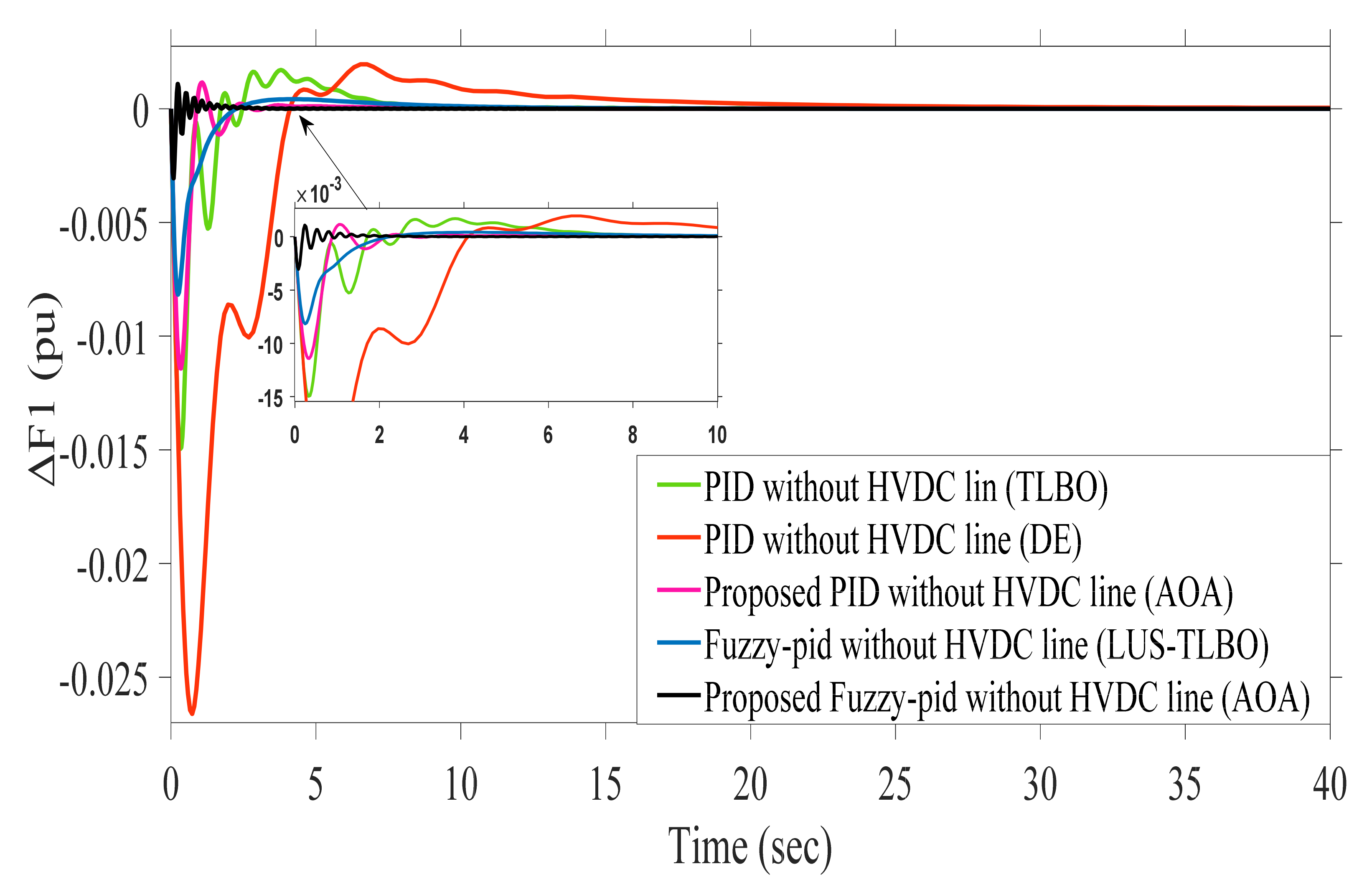
| Dynamic response of (∆F1) | 0.5510 | 1.09 | 1.7217 | 2.0347 | 1.158 |
| −8.9579 | −3.059 | −19.7259 | −26.5777 | −11.42 | |
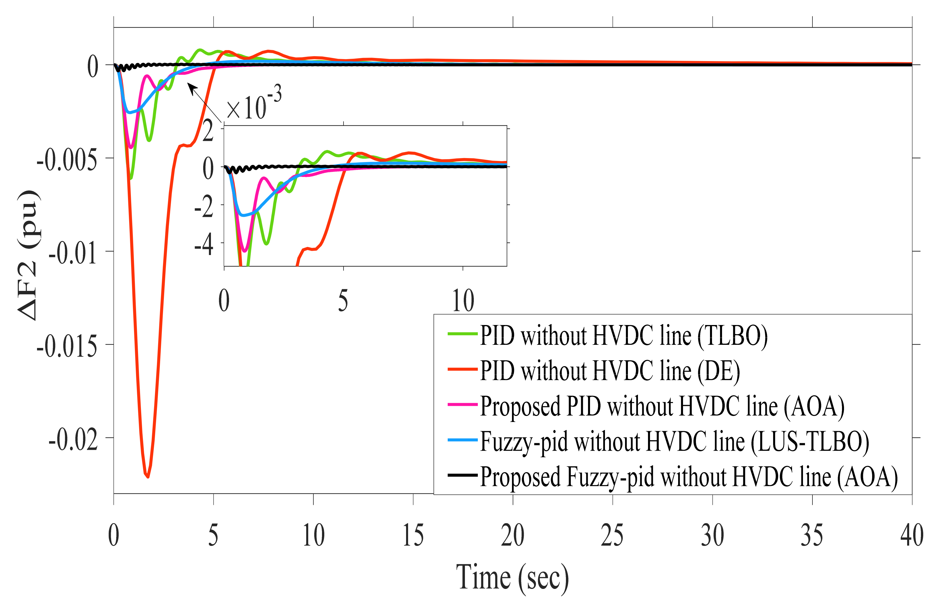
| Dynamic response of (∆F2) | 0.2119 | 0.03285 | 0.4363 | 0.7722 | 0.02096 |
| −3.0119 | −0.321 | −12.7986 | −22.1421 | −4.443 | |
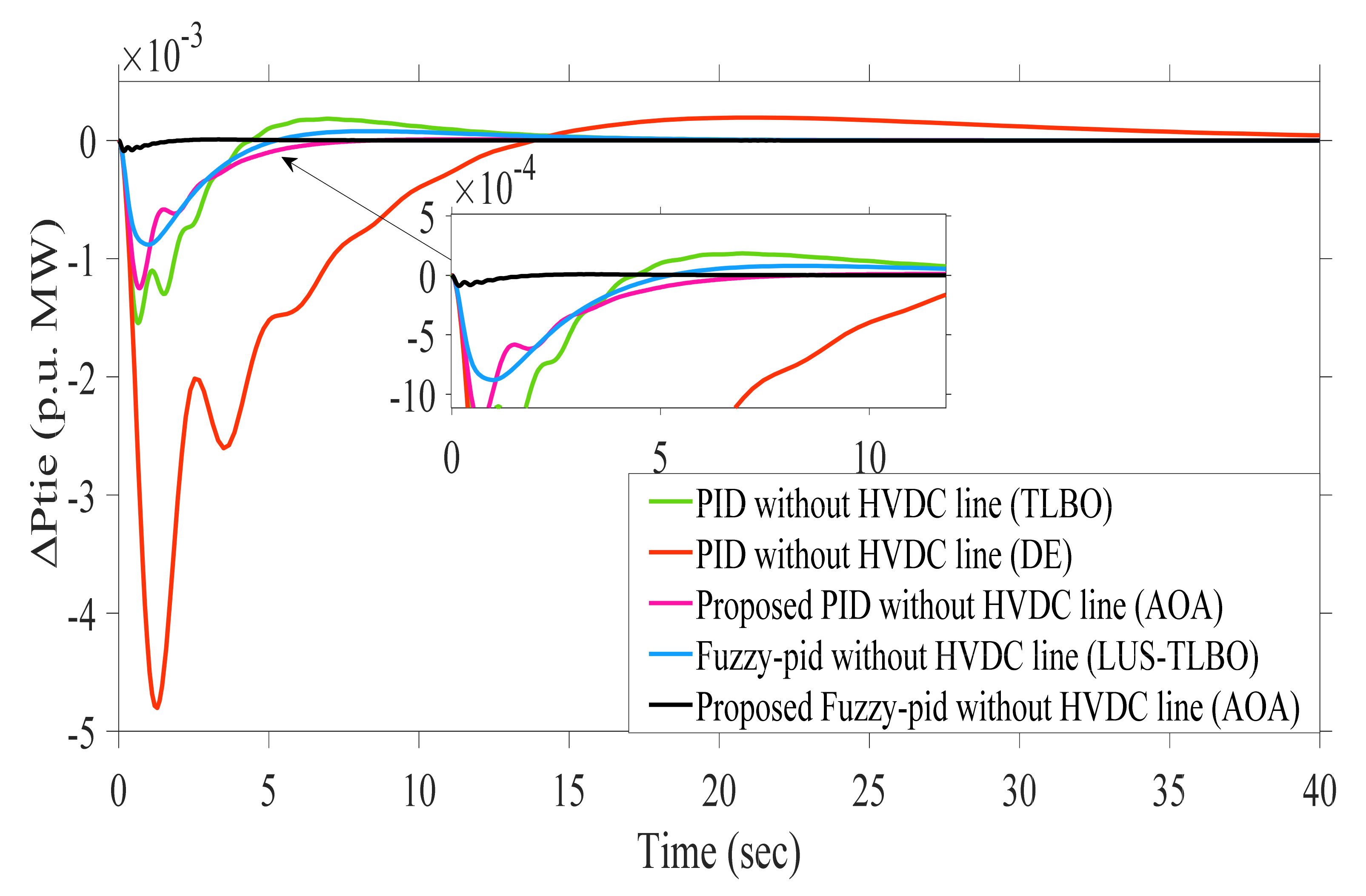
| Dynamic response of (∆Ptie) | 0.0826 | 0.008388 | 0.1712 | 0.1935 | 0.01107 |
| −0.9653 | −0.08917 | −3.0782 | −4.7595 | −1.249 |
| Controller | ||||||
|---|---|---|---|---|---|---|
| Fuzzy-PID (LUS-TLBO) | 66.29 | 72.92 | 86.4 | 72.56 | 79.72 | 57.31 |
| Fuzzy-PID (AOA) | 88.49 | 46.43 | 98.55 | 95.75 | 98.13 | 95.67 |
| PID (TLBO) | 25.78 | 15.38 | 42.2 | 43.5 | 35.33 | 11.53 |
| PID (AOA) | 57.03 | 43.09 | 79.93 | 97.29 | 73.76 | 94.28 |
| Thermal k1 k2 k3 k4 | Hydro k1 k2 k3 k4 | Gas k1 k2 k3 k4 | |||||||
|---|---|---|---|---|---|---|---|---|---|
| Fuzzy-PID (LUS-TLBO) [50] | 1.9995 1.9889 1.9975 1.9829 | 0.9668 1.2913 0.1001 1.9988 | 1.9969 1.1982 1.9867 1.9882 | ||||||
| Fuzzy-PID (AOA) | 10 9.9164 4.8295 10 | 10 0.01 4.9166 10 | 10 0.01 10 9.8531 | ||||||
| PID (TLBO) [50] | 5.0658 | 3.9658 | 2.417 | 0.7032 | 0.0220 | 0.0264 | 8.7211 | 7.4729 | 2.4181 |
| PID (DE) [49] | 1.6929 | 1.9923 | 0.8269 | 1.77731 | 0.7091 | 0.4355 | 0.9094 | 1.9425 | 0.2513 |
| PID (AOA) | 9.8739 | 1.2609 | 3.5014 | 10 | 0.0164 | 1.9788 | 1.2609 | 10 | 0.490 |
| Different Dynamic Responses | Fuzzy-PID Based LUS-TLBO OS & US × | Fuzzy-PID Based AOA OS & US × | PID Based-TLBO OS & US × | PID Based DE OS & US × | PID Based AOA OS & US × |
|---|---|---|---|---|---|
| Dynamic response of (∆F1) | 0.2809 | 0.6828 | 0.2798 | 0.3792 | 0.7707 |
| −6.7244 | −2.373 | −8.497 | −11.6667 | −10.4 | |
| Dynamic response of (∆F2) | 0.2084 | 0.02112 | 0.2138 | 0.5491 | 0.005693 |
| −1.4021 | −0.2083 | −1.624 | −2.5199 | −1.992 | |
| Dynamic response of (∆Ptie) | 0.1353 | 0.006201 | 0.1557 | 0.5474 | 0.03018 |
| −0.7292 | −0.05983 | −0.9366 | −1.8133 | −0.9134 |
| Controller | ||||||
|---|---|---|---|---|---|---|
| Fuzzy-PID (LUS-TLBO) | 42.36 | 25.92 | 44.36 | 62.05 | 59.79 | 75.28 |
| Fuzzy-PID (AOA) | 79.66 | 80.06 | 91.73 | 96.15 | 96.7 | 98.87 |
| PID (TLBO) | 27.17 | 26.21 | 35.55 | 61.06 | 48.35 | 71.56 |
| PID (AOA) | 10.86 | 103.2 | 20.95 | 98.96 | 49.63 | 94.48 |
| Different Dynamic Responses | Fuzzy-PID Based LUS-TLBO OS & US | Fuzzy-PID Based AOA OS & US | PID Based-TLBO OS & US | PID Based DE OS & US | PID Based AOA OS & US |
|---|---|---|---|---|---|
| Dynamic response of (∆F1) | 2.063 | 1.28 | 8.552 | 9.956 | 5.795 |
| −48.74 | −18.13 | −74.85 | −133.1 | −57.07 | |
| Dynamic response of (∆F2) | 0.8297 | 0.1825 | 3.981 | 3.823 | 0.1048 |
| −16.77 | −2.418 | −30.52 | −110.7 | −22.21 | |
| Dynamic response of (∆Ptie) | 0.359 | 0.06577 | 0.9155 | 0.9719 | 0.05535 |
| −5.6 | −0.8255 | −7.719 | −24.02 | −6.245 |
| Controller | ||||||
|---|---|---|---|---|---|---|
| Fuzzy-PID (LUS-TLBO) | 63.38 | 79.28 | 84.85 | 78.30 | 76.79 | 63.06 |
| Fuzzy-PID (AOA) | 86.38 | 87.14 | 97.82 | 95.23 | 96.56 | 93.23 |
| PID (TLBO) | 43.76 | 14.10 | 72.43 | −4.13 | 35.33 | 5.8 |
| PID (AOA) | 57.12 | 41.79 | 79.94 | 97.26 | 74.00 | 94.30 |
| Different Dynamic Responses | Fuzzy-PID Based LUS-TLBO OS & US | Fuzzy-PID Based AOA OS & US | PID Based-TLBO OS & US | PID Based DE OS & US | PID Based AOA OS & US |
|---|---|---|---|---|---|
| Dynamic response of (∆F1) | 37.7 | 12.69 | 59.25 | 150.5 | 46.6 |
| −1.88 | −1.526 | −8.257 | −9.28 | −0.2713 | |
| Dynamic response of (∆F2) | 47.75 | 17.1 | 73.12 | 155.4 | 56.86 |
| −2.163 | −1.106 | −8.793 | −10.92 | −0.3124 | |
| Dynamic response of (∆Ptie) | 0.06752 | 0.0361 | 0.1831 | 0.1944 | 0.01107 |
| −1.297 | −0.41 | −1.543 | −4.804 | −1.249 |
| Controller | ||||||
|---|---|---|---|---|---|---|
| Fuzzy-PID (LUS-TLBO) | 79.74 | 74.95 | 80.19 | 69.27 | 73.00 | 65.27 |
| Fuzzy-PID (AOA) | 83.56 | 91.57 | 89.87 | 89.00 | 91.47 | 81.43 |
| PID (TLBO) | 11.02 | 60.63 | 19.48 | 52.95 | 67.88 | 5.81 |
| PID (AOA) | 97.08 | 69.04 | 97.14 | 63.41 | 74.00 | 94.31 |
| Different Dynamic Responses | Fuzzy-PID Based LUS-TLBO OS & US | Fuzzy-PID Based AOA OS & US | PID Based-TLBO OS & US | PID Based DE OS & US | PID Based AOA OS & US |
|---|---|---|---|---|---|
| Dynamic response of (∆F1) | 45.73 | 16.98 | 70.37 | 124.9 | 53.66 |
| −8.18 | −3.058 | −14.98 | −26.6 | −11.43 | |
| Dynamic response of (∆F2) | 45.57 | 17.01 | 70.31 | 124.8 | 53.68 |
| −2.586 | −1.738 | −7.94 | −22.13 | −5.42 | |
| Dynamic response of (∆Ptie) | 5.233 | 0.7004 | 7.246 | 22.57 | 5.867 |
| −5.199 | −0.7178 | −7.257 | −22.60 | −5.874 |
| Controller | ||||||
|---|---|---|---|---|---|---|
| Fuzzy-PID (LUS-TLBO) | 69.25 | 63.39 | 88.31 | 63.49 | 77.00 | 76.81 |
| Fuzzy-PID (AOA) | 88.50 | 86.41 | 92.15 | 86.37 | 96.82 | 96.90 |
| PID (TLBO) | 43.68 | 43.66 | 64.12 | 43.66 | 67.89 | 67.89 |
| PID (AOA) | 57.03 | 57.04 | 75.51 | 56.99 | 74.01 | 74.00 |
Publisher’s Note: MDPI stays neutral with regard to jurisdictional claims in published maps and institutional affiliations. |
© 2021 by the authors. Licensee MDPI, Basel, Switzerland. This article is an open access article distributed under the terms and conditions of the Creative Commons Attribution (CC BY) license (https://creativecommons.org/licenses/by/4.0/).
Share and Cite
Elkasem, A.H.A.; Khamies, M.; Magdy, G.; Taha, I.B.M.; Kamel, S. Frequency Stability of AC/DC Interconnected Power Systems with Wind Energy Using Arithmetic Optimization Algorithm-Based Fuzzy-PID Controller. Sustainability 2021, 13, 12095. https://0-doi-org.brum.beds.ac.uk/10.3390/su132112095
Elkasem AHA, Khamies M, Magdy G, Taha IBM, Kamel S. Frequency Stability of AC/DC Interconnected Power Systems with Wind Energy Using Arithmetic Optimization Algorithm-Based Fuzzy-PID Controller. Sustainability. 2021; 13(21):12095. https://0-doi-org.brum.beds.ac.uk/10.3390/su132112095
Chicago/Turabian StyleElkasem, Ahmed H. A., Mohamed Khamies, Gaber Magdy, Ibrahim B. M. Taha, and Salah Kamel. 2021. "Frequency Stability of AC/DC Interconnected Power Systems with Wind Energy Using Arithmetic Optimization Algorithm-Based Fuzzy-PID Controller" Sustainability 13, no. 21: 12095. https://0-doi-org.brum.beds.ac.uk/10.3390/su132112095